Review

Magnetic Materials and Systems: Domain Structure Visualization and Other Characterization Techniques for the Application in the Materials Science and Biomedicine

by
Roberto Nisticò
1,†,
Federico Cesano
2 and
Francesca Garello
3,*
1
Department of Applied Science and Technology DISAT, Polytechnic of Torino, C.so Duca degli Abruzzi 24, 10129 Torino, Italy
2
Department of Chemistry and NIS Centre, University of Torino, Via P. Giuria 7, 10125 Torino, Italy
3
Molecular and Preclinical Imaging Centers, Department of Molecular Biotechnology and Health Sciences, University of Torino, 10126 Torino, Italy
*
Author to whom correspondence should be addressed.
Current address: Independent Researcher, Via Borgomasino 39, 10149 Torino, Italy.
Submission received: 23 September 2019 / Revised: 28 December 2019 / Accepted: 31 December 2019 / Published: 17 January 2020

Abstract

:
Magnetic structures have attracted a great interest due to their multiple applications, from physics to biomedicine. Several techniques are currently employed to investigate magnetic characteristics and other physicochemical properties of magnetic structures. The major objective of this review is to summarize the current knowledge on the usage, advances, advantages, and disadvantages of a large number of techniques that are currently available to characterize magnetic systems. The present review, aiming at helping in the choice of the most suitable method as appropriate, is divided into three sections dedicated to characterization techniques. Firstly, the magnetism and magnetization (hysteresis) techniques are introduced. Secondly, the visualization methods of the domain structures by means of different probes are illustrated. Lastly, the characterization of magnetic nanosystems in view of possible biomedical applications is discussed, including the exploitation of magnetism in imaging for cell tracking/visualization of pathological alterations in living systems (mainly by magnetic resonance imaging, MRI).

Graphical Abstract

1. Introduction

Since the early beginning of our society, magnetism catalyzed the attention of scientists worldwide due to its intrinsic capability to naturally attract/move inanimate matter [1,2]. However, it is with the discoveries of Pauli’s exclusion principle and Heisenberg’s quantum theory that the “Modern Theory of Magnetism” was finally coined in the 1920s, unveiling the strict correlation existing between magnetism and the number/motion of electrons [3]. From here, the scientific community reached several steps forward toward the production of more and more advanced magnetic (nano)materials and (nano)systems that found applications in many useful scientific/technological fields, such as in (bio)medicine [4,5], drug-delivery [6,7,8], imaging [9,10,11], spintronics and electronics [12], data storage [13], robotics [14,15], environmental remediation processes [14,15,16,17,18,19], (nano)engineering [20,21,22], and miniaturized devices [23].
Due to the growing interests around the exploitation of magnetic (nano)materials, a detailed comprehension of this phenomenon is becoming more and more important, if not crucial. Many characterization techniques are used daily to qualitatively and/or quantitatively determine the magnetic response in materials [1,24]. However, being very specific, these techniques could be unfamiliar to a wide audience. The analysis of the state-of-art pointed out that the scientific literature is very rich in reviews focused on the production/testing of magnetic materials in various fields [25,26,27,28], assuming as elementary the comprehension of the adopted characterization techniques. On the basis of the authors’ experience, a superficial (and simplistic) interpretation of these data could leave to misleading (and in some cases incorrect) analysis [1]. In this context, it is worthy of note that there are many previous publications related to these subjects, including reviews and books. Some of them [24,29,30,31,32,33,34,35,36] can be still considered as “classical” as they are constantly used in many laboratories around the world.
Therefore, aim of this review is to provide (in a simple, but precise way) a technical summary of the main relevant characterization techniques mandatory for determining magnetism-related phenomena in (nanoscopic) materials and systems and some of the most recent advances in the field, new methods and approaches. Obviously, the number of techniques exploitable for this purpose can be extremely various and it is almost impossible to provide an enough-detailed analysis of all the possible variants and approaches (for a much detailed comprehension of each technique, readers should refer to dedicated papers and the afore mentioned literature). Thus, for the sake of clarity, authors have decided to focus the discussion on some relevant methods illustrated in the literature, in correlation also with their peculiar expertise. Hence, the following paragraphs were organized introducing three main topics: A brief introduction dedicated to the determination of the magnetization (hysteresis) curves (fundamental for recognizing not only the level of magnetism in materials/particles, but also the types of magnetism, vide infra) and their interpretation, the visualization and description of magnetism at mesoscale (including the correlation between nanomagnetism and morphology), and the exploitation of magnetism in imaging for cell tracking or visualization of pathological alterations in living systems (mainly by magnetic resonance imaging, MRI). Concerning this last topic, a particular attention will be devoted to the characteristics that magnetic systems shall possess to be safely and successfully employed in living organisms (both in vitro and in vivo).
The final goal of this review is to draw guidelines beneficial for the correct comprehension of the magnetism-related literature, even for not insiders, as well as to point out how a magnetic system should be designed and characterized in order to be suitable for in vivo applications. The multidisciplinary approach here presented is the result of different viewpoints, in particular the merging of the physical and morphological peculiar characteristics of magnetic nanosystems applied to the biomedical field. To facilitate the document’s readability, specific case studies were taken as reference examples, key points and criticalities highlighted. With this work, the authors’ hope is to have unequivocally disclosed any possible complex aspects in the field, thus facilitating the proliferation of interesting (and optimistically outstanding) future studies.

2. Magnetism and Magnetization (Hysteresis) Curves

On the basis of the “Modern Theory of Magnetism”, the appearance of strong magnetic phenomena in materials and molecular structures is due to the presence of chemical elements with a particular electronic configuration, namely: Iron (Fe), nickel (Ni), cobalt (Co), manganese (Mn), chromium (Cr), and some rare earth metals [37]. Independently from the types of magnetism, the most common method for evaluating the magnetic response in materials is the determination of the magnetization (hysteresis) curves by means of a magnetometer [38]. Even if there are several configurations of magnetometers, the most common one is the vibrating sample mode (VSM). In a VSM magnetometer, the test specimen is subjected to a magnetization-demagnetization loop process by varying the external magnetic field applied. The material’s magnetization, intended as the vector field which indicates the density of magnetic moments (i.e., vector relating the alignment on the material by applying an external magnetic field with respect to the field vector), is measured indirectly as electric current variation/formation of the inductive coils surrounding the sample-holder (it should be remembered that both electric and magnetic fields are strictly correlated between each other since being orthogonal). According to the “IEEE Magnetic Society” [39], magnetization is expressed in two different forms: as total (volume) magnetization (M, an expression of the magnetic moments per unit of volume, units of measurement A/m for the International System of units (SI) and emu/cm3 for the Centimeter-Gram-Second system of units (CGS)) and as total (mass) magnetization. Another useful property is the magnetic induction (B, magnetic flux density in the sample, units of measurements T for SI and G for CGS) [40]. These units are correlated between each other [41] according to the Equation (1) (derived from the Maxwell’s equation):
B = µ0 (H + M)
where H is the applied magnetic field (external magnetic stimulus, units of measurement A/m for SI and Oe for CGS) and µ0 is the vacuum permeability (a constant value equal to 4π × 10−7 H/m, as defined in SI). Sometimes, it is better to remind that the CGS system is preferred respect to the SI, thus for any clarification concerning the units of measurements of magnetic properties, please refers also to [1]. At this point, it can be useful for the entire discussion, introducing some important physical quantities with their definitions. In details, the saturation magnetization (Ms) is the maximum magnetic moment induced by an external magnetic field applied, the intrinsic coercivity (Hci) is the reverse field required to bring the magnetization M to zero, and the magnetic remanence (Mr) is the residual magnetization at zero external magnetic field (H = 0) [40].
The main differences between these two configurations (namely, M vs. H and B vs. H) are related to both shapes and physical quantities obtained [39]. As shown in Figure 1, Br is the residual induction at H = 0, whereas Hc is the coercivity (or the reverse field necessary to bring the B to zero).
The more enlarged the hysteresis loop (such as in the case of hard-magnets, vide infra), the higher the discrepancies between the two coercivity values (Hc and Hci). This suggests that when the hysteresis loop becomes very narrow (or negligible), the two representations of the magnetization profiles tend to be similar, thus justifying in some ways the wrong interchanges mostly found in the literature. For the sake of clearness, from here only M vs. H curves were considered.
Figure 2 reports the possible different profiles of magnetization (hysteresis) curves depending on the form of magnetism. Being more precise, there are five relevant forms of magnetism, and among these the more intense (and, consequently, macroscopically-detectable by human eyes without specific techniques) are only two: ferromagnetism and ferrimagnetism. Superparamagnetism is a thermal/size-induced particular response of the previous two forms of magnetism, while diamagnetism, paramagnetism, and antiferromagnetism are weaker forms of magnetism.
Ferromagnetism consists in a spontaneous magnetization/alignment of the matter (even without applying an external magnetic stimulus) of the order of ca. 106 A/m. Ferromagnetism is generated by the self-alignment of the unpaired (same-spin) electrons forming the material. Since this phenomenon is energetically favored only at short-range, it is reflected by the formation of randomly aligned magnetic domains. In fact, at the macro level, the energetically favored anti-alignment organization of adjacent poles is still the more predominant one. Vice versa, in presence of an external magnetic field applied, domains aligned themselves according to the external magnetic field directions [42].
Interestingly, Fe, Ni, and Co (3d metals) are the only three pure elements with ferromagnetic properties at room temperature (RT). Ferromagnetic materials are characterized by having a well-defined Ms, and high Hci and Mr.
Additionally ferromagnetic materials can be classified as hard (permanent magnet, with high Hci) and soft (easily (de)magnetized, with low Hci) [1,35,43,44]. Lastly, the high values of Hci and Mr are an expression of the capability of ferromagnetic materials of retaining a memory of their magnetic history. Moreover, ferromagnets are sensible to temperature. In fact, by increasing the temperature above the Curie point (a critical temperature value typical of each magnetic material), ferromagnetic materials start behaving as paramagnetic materials (vide infra), with formation of random domains [45]. This reversible phenomenon is due to disordered motions of electrons caused by an overall increment of entropy in the system. From the magnetization curve in Figure 2, the formation of the hysteresis phenomenon is attributable to a certain magnetic anisotropy due to structural parameters (such as: Crystal structure, shape/dimensions of grains/particles, stress/tension, interaction with (anti)ferromagnetic materials), and this is particularly strengthened in the case of hard-magnets, which show high Hci (see [1,35] and references therein). Figure 3 reports the schematic view of a ferromagnetic system in absence and in the presence of an external magnetic field applied.
Interestingly, Fitta and co-workers [46] reported the layer-by-layer deposition of a bilayer system composed of hard Ni3.38[Fe(CN)6]2·nH2O (indicated as NiFe) and soft Ni3.1[Cr(CN)6]2·nH2O (indicated as NiCr) ferromagnetic compound. Figure 4 reports the magnetic hysteresis loops at 2 K for bilayer sample against their orientations respect to the direction of external magnetic field (namely, 0°, 45°, and 90°). As reported in the figure, when sample is parallel oriented (0°), a two-phase hysteresis was observed: (i) A drop in magnetization by decreasing the magnetic field (at small value) due to the presence of the NiCr layer (soft-magnet), and (ii) a pronounced hysteresis loop due to the presence of the NiFe layer (hard-magnet). By varying the orientation toward perpendicular (90°), the magnetization process is much more gradual. This variation of the magnetization curve with respect to the film orientation is attributable to the anisotropic properties of the NiCr layer: Parallel orientation indicates easy magnetization direction, whereas perpendicular one indicates a hard magnetization direction.
Ferrimagnetism is a very particular form of magnetism. This phenomenon occurs in materials organized into two interpenetrating structures located at the different sublattice, showing an anti-alignment of spins with not-equal magnetic moments, thus resulting in an overall valuable magnetic moment below the Curie temperature [47]. Analogously to ferromagnetic materials, ferrimagnetic systems exhibit spontaneous magnetization, hysteresis loop, and a Curie point [1,35]. Typical ferrimagnetic systems are magnetite (Fe3O4, a mixed ferrous-ferric oxide with the spinel crystal structure AB2O4) and other ferrites (Fe-containing mixed oxides with the spinel crystal structure MFe2O4, with M being a general metal). For the sake of clarity, Figure 5a depicts the spinel crystal structure of MnV2O4, where the two substructures are made by the V-octahedral and Mn-tetrahedral sites [48]. Interestingly, by making a comparison between Figure 5b and Figure 5c, it is possible to appreciate the effect induced by the temperature variation on the phase crystal structure (i.e., cubic-to-tetragonal transition during cooling) and consequently on the organization of the magnetic structure (from collinear to non-coplanar ferrimagnetic order). Additionally, also rare earth alloys (eventually in combination with magnetic transition metals) are widely adopted as permanent magnets [49,50,51]. Among the lanthanides, the most used ones are the neodymium (Nd)-based magnets [52] and the samarium (Sm)-based ones [53].
On the contrary, paramagnetism is the tendency of materials of displaying a net magnetic moment if exposed to a magnetic field. As paramagnetism comes from the partially-filled orbitals, either forming bands or being localized, only certain systems lead to paramagnetic properties, in principle metals and insulators having localized moments. Macroscopically, when paramagnetic materials are subjected to an external magnetic field, they tend to align following the magnetic field direction, giving both magnetization and susceptibility slightly positive (as depicted in Figure 2) [54]. However, it must be noticed that paramagnetism might be associated also to other forms of magnetism. For example, Preller and co-workers [55] reported the production of FePt nanomaterials. As summarized in Figure 6, Fe3Pt nanomaterial shows clearly a soft magnetic behavior (Figure 6a), whereas FePt3 predominantly exhibits a paramagnetic character associated with traces of ferromagnetism due to the presence of a minor ferromagnetic phase (Figure 6b).
As reported in a previous study [1], superparamagnetism is a particular form of paramagnetism below the Curie point in both ferro/ferri-magnetic materials when organized in the shape of small “single-domain” nanoparticles (thus it is a thermal and size dependent particular response of ferro/ferri-magnetic materials) [24]. In detail, since single-domain nanoparticles (with dimensions below 20 nm size) can randomly change their directions of the magnetization with temperature/time fluctuations, the average magnetization value of such systems in absence of an external magnetic field is close to zero [10]. In presence of an external magnetic field, nanoparticles align following the magnetic field direction as for paramagnetic materials. However, due to their ferro/ferri-magnetic origin, such nanomaterials show very high magnetic susceptibility (larger than common paramagnetic materials, i.e., “super”paramagnetism) and absence of hysteresis (Hci-values close to zero, and Mr-values very low) [38].
Conversely to paramagnetism, diamagnetism is the capability of repel/oppose to an applied external magnetic field, due to the absence of unpaired electrons, giving weak negative magnetization and susceptibility [56]. This phenomenon is widely exploited for the levitation/floating of bodies, such as in the case of Maglev train (i.e., superconductors are perfect diamagnets).
Finally, analogously to ferrimagnetism, antiferromagnetism consists in magnetic phenomenon generated by the presence of two interpenetrating structures characterized by having an equal antialignment of electrons’ spins, and consequently an overall zero magnetization at the macroscale. This phenomenon is evident at low temperature, whereas at temperature higher than the Néel point it is registered the antiferromagnetism-to-paramagnetism transition (in analogy to Curie transitions of ferromagnetism) [1,24].
Figure 7 reports a summary of the main features of the principal different forms of magnetism [57]. On the basis of the state-of-art literature, several case studies reported the exploitation of magnetization (hysteresis) curves for the determination of the magnetic properties of materials, making this technique an extremely powerful method for investigating magnetic systems.
Paulo et al. [58] studied the formation of metallic (Ni, Fe, Co) ferromagnetic nanotubes via chemical electrodepositing using porous polycarbonate membranes as hard-templating system. Magnetic curves were used for evaluating not only the magnetic response, but also to determine the effect of parallel/perpendicular fields with respect to saturation, remanence and coercivity. Another interesting study is the one reported by Venkata Ramana and co-workers [59], focused on the evaluation of Fe-doping on BTCZO, acronym of (Ba0.85Ca0.15)(Ti0.9Zr0.1)O3. Evidences confirmed that undoped BTCZO is diamagnetic, whereas the Fe doping caused a gradual evolution toward ferromagnetism. Peixoto et al. [60] produced CoFe2O4 nanoparticles embedded inside a TEOS-derived SiO2 matrix via sol–gel (for sol–gel processes, refer to [61,62]) and evaluated the magnetic properties by fixing the temperature at either 5 K or 100–200 K confirming a superparamagnetic regime. In this context, it is important to point out that several cases studies reported magnetization curves detected at different temperatures (going from cryogenic conditions to temperature values above/below the Curie point), and this is fundamental for evaluating specific magnetic transition in the (nano)material/system analyzed. Wang et al. [63] reported a comprehensive study focused on the magnetic response evaluation in perovskite crystal systems. In recent studies, magnetic composite nanomaterials made by either magnetite/chitosan [64,65] or magnetite/humic-like substances [18,66] isolated from municipal biowaste [67] were thermally-converted via pyrolysis at 550–800 °C.
The analysis of the magnetization curves resulted to be fundamental to indirectly understand the chemical modifications induced by the pyrolysis treatment monitoring the magnetic properties in the final material. In detail, it should be remembered that magnetite is converted into wustite (FeO) upon heating (at 575 °C) under inert atmosphere and in the presence of a carbon source (e.g., chitosan or the humic-like substances). Since instable, FeO disproportionates, giving metallic Fe and magnetite phases. The analysis of the magnetization curves pointed out that pristine magnetic nanocomposites (containing magnetite) have saturation values lower than bare magnetite. Pyrolysis at temperatures below 575 °C affects only the magnetization profiles with an increment of saturation, coercivity and remanence due to the consumption of the organic layer toward the formation of carbon. Conversely, pyrolysis at temperature higher than 575 °C caused a remarkable increment of the saturation level (even higher than the reference bare magnetite), suggesting the growth of a different magnetic phase, namely Fe (which is ferromagnetic). Moving toward the organic-based and molecule-based magnets, Miller [68] resumes the main findings obtained for the family of [TCNE]●−-based magnets. Namely, by modifying the chemical structure of this family, different forms of magnetism were registered, such as: ferromagnetism for [FeIII(C5Me5)2]●+[TCNE]●− and V[TCNE]2, weak ferromagnetism for Li+[TCNE]●−, ferrimagnetism for MnII(TCNE)3/2(I3)1/2, and antiferromagnetism for MII(TCNE)[C4(CN)8]1/2 (with M = Mn, Fe). In all cases the analysis of the magnetization (hysteresis) curves resulted fundamental not only for recognizing the form of magnetism, but also for the evaluation of the magnetic properties. Shirakawa et al. [69] measured the magnetic properties of an organic radical ferromagnet, β-p-NPNN, below and above the Tc. Interestingly, in their study Shum and co-workers [70] reported evidences of pressure-induced metamagnetic-like transition from antiferromagnetism to ferromagnetism for [Ru2(O2CMe)4]3[Cr(CN)6] system. Lastly, also carbon allotropes (mostly 2D organic systems [71,72,73] and carbon nanotubes [74,75]) show unique optoelectronic and magnetic properties. In most cases, for practical applications the doping of these materials with heteroatoms (in particular to extend their magnetic ordering at long-scale) is mandatory. In this context, Tucek and co-workers [76] synthesized flourographene (thus introducing F atoms in the carbon texture) with hydroxyl groups showing antiferromagnetic ordering. However, in the literature it is widely questioned the possible role of metal impurities (Fe, Ni, Co) derived from the synthesis of such carbon allotropes (and derivatives) in their magnetic response [77].
At the end of this section, authors suggest the following specific literature for further deepening the theory and influence of parameters affecting the magnetization (hysteresis) curves [32,34,78,79].
Moreover, magnetization processes (and equipments) can be classified into quasi-static (DC) or dynamic (AC) processes [80,81]. In detail, DC magnetometry consist in magnetizing the samples and registering the magnetic moment by applying a constant magnetic field (one above all the VSM set up). On the contrary, in the AC magnetometry, an AC magnetic field is superimposed on a DC field, thus causing a time-dependent magnetic moment, which allows the magnetization without moving the sample. In the AC magnetometry, at low frequencies the M vs. H curve is very similar to the DC one and the slope of the M vs. H profile is the susceptibility. The main advantage of this technique is the high sensitivity, thus making detectable even very small magnetic variations. At high frequencies, instead, the magnetic moment registered differs from the DC one due to dynamic effects. For these reasons, the AC magnetic susceptibility is defined by two parameters: The magnitude and the phase shift, which are sensitive to thermodynamics phase changes or temperature-induced magnetic transitions (e.g., the superparamagnetism and superconductivity as well as the determination of the Curie/Néel point). Interestingly, by plotting the magnetization against the temperature or the susceptibility against the temperature, one can determine the magnetic phase transition (i.e., Curie/Néel point). For completeness, authors suggest the following references dedicated [82,83,84,85,86].
Furthermore, another very promising equipment that deserve the attention of experts is the SQUID (acronym of Superconductive QUantum Interference Device), which is an extremely sensible magnetometer widely exploited for the determination of very weak magnetic field (below 10−18 T). SQUIDs can be classified as either direct current (DC) or radio frequency (RF), and can be integrated into chips. In general SQUIDs are made by Nb or Pb alloys operating at temperature closed to the absolute zero (i.e., the system deserves being cooled down with liquid He or N2). The analysis of the literature revealed that SQUIDs are widely used for biology studies (due to the very weak intensity of the magnetic fields registered) as well as detectors in magnetic field imaging (MFI) or in relaxometry (vide infra), however a complete and detailed discussion on this very specific technique is out from the scope of this review, which instead is focused on the technique easily findable in a magnetism-dedicated laboratory. For more detailed discussion, please consider the following literature and references therein [87,88,89,90].

3. Imaging of the Domain Structure and Beyond

The hysteresis properties, as defined in the previous paragraph, represent bulk characteristics or integrated amounts of the magnetic character of a sample as a whole. On the other hand, the magnetization is in principle a vector (and not a scalar quantity) and could be locally identified at the mesoscale. In addition, magnetic nanoparticles for both fundamental studies and technologies have been intensively explored for the past two decades. Different from the bulk counterparts, nanoparticles (NPs) with magnetic properties show unique magnetism characteristics, enabling the tuning of their magnetism by methodological nanoscale approaches. In a recent review, Wu et al. [91] have summarized the major synthetic procedures and the application fields of various magnetic NPs, including metals, metallic alloys, metal oxides, and multifunctional NPs.
Microscopies dedicated to magnetic investigation are perfectly suited for unravelling all these local magnetic properties, making available on the basis of the magnetism principles a set of information that can be adopted for improving and designating new materials or for the creation/modification of magnetic domains (spintronics) as well. For example, when dimensions of a system go down to the nanoscale the uniform magnetization hypothesis is unreliable and properties become exclusive. Local regions with uniform magnetization (i.e., magnetic domains), their boundary structure (i.e., domain walls), the directions of magnetization and the magnetization extent can be revealed under both static or dynamic conditions (i.e., magnetization reversal and time-reversal behaviors) from the cryogenic cooling to high temperature [92,93,94,95].
Electrons, photons, neutrons and X-rays are four kinds of modern probes offering a plethora of opportunities for the investigation of the magnetic properties (Figure 8). Besides other exciting properties, the aforementioned probes make it possible to visualize magnetic domains and structures, obtaining often quantitative results. The imaging of the magnetic domain structure is, for a fact, a way to reveal the local magnetic properties of materials from the macroscale down to the nanoscale. Since the publication of the comprehensive review on “Magnetic domains” by Craik and Tebble [31], dated 1961, new techniques and materials became available, while new insights were evidenced and perspectives appeared over the years. The method of observation can provide today useful insights also into the origin and reversal mechanisms of the magnetization, the sample magnetic vortex structures, that are all of a great importance from a fundamental point of view of the application, for example spintronics and other technologies. Shrewd interpretation of the variety of magnetic visualization techniques is used in this section both to begin the readers who are not familiar with these techniques and to help those more expert to figure out their own matter.
This review section is intended to be a survey around the topical methods for magnetic domain/domain structure observations and some of the recent findings. The appraisal of the today’s significance in the corresponding field is discussed. The theories and principles of magnetism, including Weber’s molecular and domain, and magnetic field theories are the background to this discussion.
Therefore, all aspects of magnetic structural characterization are not entirely covered, but a few techniques to be employed in modern investigations of magnetic systems in a wide dimensional range, from macro/microstructures (i.e., materials), to nanoparticles, molecular assemblies and single-molecule magnets are discussed. As each technique has its own advantages and disadvantages, the present review aims at helping researchers to select the most appropriate method for their purposes, but before discussing the techniques in more detail, a set of general comments for the imaging methods is needed. Firstly, almost all of the family of the visualization methods are firmly restricted to the topmost layer(s), a few micro- or nanometers deep in the matter, an area dominated by magnetic characteristics located at the surface. Nothing is associated with the properties of the inner portion that should be investigated by other characterization techniques more precisely dedicated to bulk magnetic properties (see the first section of this review). Secondly, some methods usually need a cleaned, smoothed and defect-free surface, and/or the operational conditions (i.e., vacuum) could be far from working conditions. Thirdly, the imaging of the domain walls in some methods could be affected by preparation (i.e., use of magnets to collect the particles that can affect their in-the-plane or transversal orientations). Fourthly, a compromise between sensitivity and resolution, must be taken under consideration and a multi-technique approach would be valuable.
As for characterization techniques, however, it is not surprising that in most papers a multi-technique approach is reported. The complementary investigation, typically adopted in materials science by means of microscopies or other visualization techniques with spectroscopies and textural analysis, overcomes the intrinsic limitation of individual methods and offers complementary details for assessing the correlation between morphology, structure and other properties of complex or nanostructured materials [11,21,44,96,97,98,99,100,101,102,103,104,105,106,107,108].
For the sake of comparison, a summary of the visualization techniques discussed in this review is detailed in Table 1. Such table should be intended as an overview of the possible investigation approaches and it offers a broad outline of the different characterization methods.

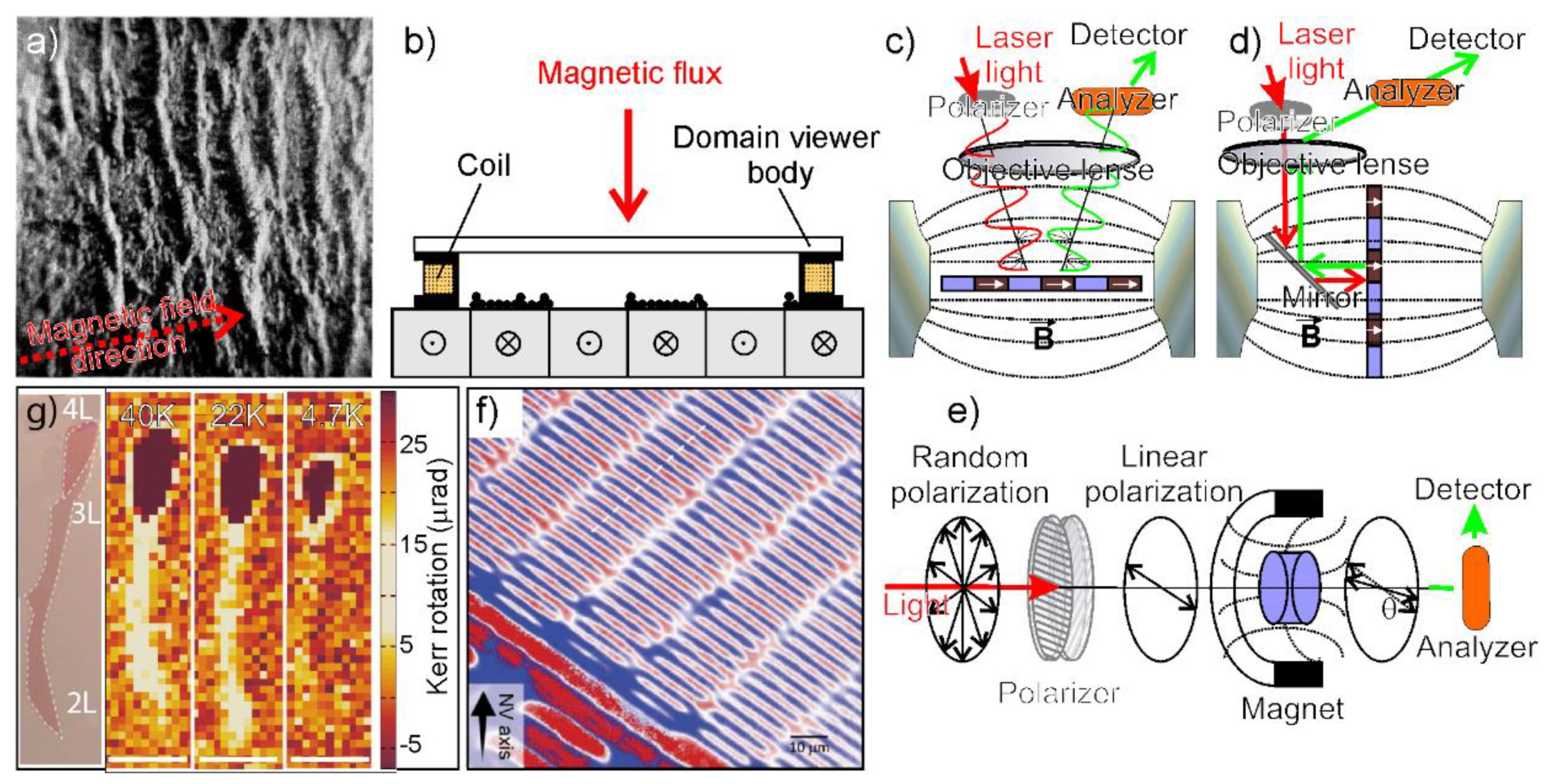
3.1. Powder Pattern Imaging

It is easy to observe characteristic domain structures in materials by the Bitter powder imaging technique. Bitter patterns, firstly observed by Hamos and Thiessen [131], and Bitter [132] in 1931, involve a ferrofluid (or a colloidal suspension of small Fe/iron oxides particles), placed on the surface of a ferromagnetic material, which outlines the boundaries of the magnetic domains. The magnetic walls, having a higher magnetic flux than the regions located in the domains, can be visualized by the optical microscopy (Figure 9a) or better implemented into a device, where a coil generating a magnetic field helps for the observation (Figure 9b).
Nonetheless, no relationships to the grain structure can be obtained. Although the method is quick and simple, the investigation of the domain structure by the conventional Bitter pattern technique could be difficult for soft magnetic materials, complex domain structures, and even impossible for the smaller domain structures [134,135]. Furthermore, as the method is firmly a stray field decoration technique, patterns direction and magnitude of the magnetization are not available. Lastly, the Bitter powder pattern of Néel-type domain walls was found much more visible than that of a Bloch-walled structure [136]. Finally, as the method commonly gives more reliable results with high coercivity magnets or perpendicularly magnetized specimens, a small magnetic field applied perpendicularly to the sample surface is frequently used to increase the image contrast. Although old, Bitter technique has been recently improved. In a recent paper, Simpson et al. [122] have reported the magneto-optical response of negatively charged nitrogen-vacancy (NV) centers in diamond to quantitatively image the stray magnetic fields in thin ferromagnetic films with time and spatial resolutions of 20 ms and 440 nm. The technique, potentially working with any magnetic material with a stray magnetic field, can be operated under ambient conditions by placing the specimen in contact with the diamond imaging chip (see also in Section 3.10). In another paper, Sonntag et al. [137] investigated a deformed steel sample (S235JR) with composition: Fe-0.073C–0.47Mn–0.19Si–0.26Cu–0.12Cr–0.069Mo–0.18Ni to image macroscopic deformation gradients. The authors also concluded that geometrical features of the stress curves can be determined quantitatively by Bitter contrast images, including dimensions of different deformation regions and asymmetries.

3.2. Magneto-Optical Imaging

The interaction between polarized light and the magnetization of a material is generally a weak signal, but informative enough to attain the visualization of the domain. Though the principles of the magneto-optical interactions could be relatively difficult, the method is based on the change in polarization of incident light as it is reflected (or transmitted) by a magnetic material at the most elementary level. The magneto-optical effect in reflection mode is usually referred to as Kerr effect (MOKE), while in transmission mode as the Faraday effect. Precisely, the MOKE technique can be also divided into three different geometries: Longitudinal, polar, and transverse magneto-optical Kerr effect [138]. In the longitudinal MOKE geometry (Figure 9c), the magnetic field is applied in the plane of the sample and domains will tend to be oriented along the magnetic field direction. The light engendered by a laser passes firstly through a polarizer, then in an objective lens focusing the sample. On the other hand, the incident polarized light reflects off the sample surface, being rotated by the interaction between the polarized beam and the magnetic domain structure of the sample. The magnitude of the rotation is proportional to the local magnetization. The reflected signal passes through an analyzer so that the Kerr rotation signal can be measured. The degree of Kerr rotation can be used to determine the orientation and magnitude of the local magnetic domain. In the polar MOKE geometry, out-of-plane with respect to the sample plane the magnetic field is applied, and the resulting magnetization is transverse to the sample plane (Figure 9d). The incident laser excitation, perpendicularly aligned to the sample plane, is usually adopted for collecting the maximum signal. As in the longitudinal geometry, the polarization of incident laser light is rotated by a small degree when it reflects off from the surface of the magnetic sample. The magnitude of the Kerr rotation is related to the strength and orientation of the local magnetic domain. In fact, when the light beam is incident perpendicular to the surface in the Faraday or Kerr configurations, domains magnetized normal to the surface plane are imaged.
For the visualization, a light microscope with a working distance (WD) of several centimeters is required. The optical path allows to allocate a polarizing filter between the sample and objective lens, but owing to the relatively large WD, the resolution is slightly limited. To gain Kerr microscopy images closer to the limit resolution (300–500 nm), a relatively small distance between sample and objective lens, typically one millimeter or less (even possible if the sample is in the air), is required. Notwithstanding these techniques can be very sensitive, usually no quantitative determinations of the magnetization are provided. Nevertheless, the combination with a dedicated setup (e.g., the application of a bias potential) can provide quantitative results [122] (Figure 9f). Recent experimental studies on low-dimensional nanostructures (e.g., transition metal dichalcogenides, and graphene) show the potential of the magneto-optic effects to gain magnetic information on 2D systems. Gong and co-authors [133] reported the magnetic imaging of few-layered Cr2Ge2Te6 crystals, as obtained at 40 K, 22 K, and 4.7 K (Figure 9g). Taking into consideration these images, the authors concluded that, although the magnetic properties are strongly suppressed by thermal fluctuations, due to the magnetic anisotropy a long-range ferromagnetic order can be observed in 2D crystals. Furthermore, Kerr rotation images were recently used by Lee et al. [139] to describe magneto-electric properties of 1-layer MoS2-based devices to be employed as integrated photonic and spintronic devices. Together with the domains visualization under static or dynamic conditions, the motion of magnetic domain walls driven by magnetic field pulses or current pulses can be studied by time-resolved or transient MOKE spectroscopy [140]. MO Faraday technique has been adopted by Kustov et al. [141] to obtain thermal imaging with high sensitivity, with micrometer as spatial and with millisecond as temporal resolutions, by using BiLu2Fe4GaO12 ferrimagnetic film as a pyro-magneto-optical detection layer. Dikson et al. [111] adopted high-resolution optical techniques (confocal microscopy and scanning near-field optical microscopy: SNOM) for imaging the magnetic domains in ferromagnetic thin films based on gadolinium–iron–cobalt (GdFeCo) and terbium–iron–cobalt (TrFeCo). The authors showed that the magneto-optical resolution in the near-field measurements depends on the film thickness and it is affected by the diffraction on magnetic domains throughout the film.

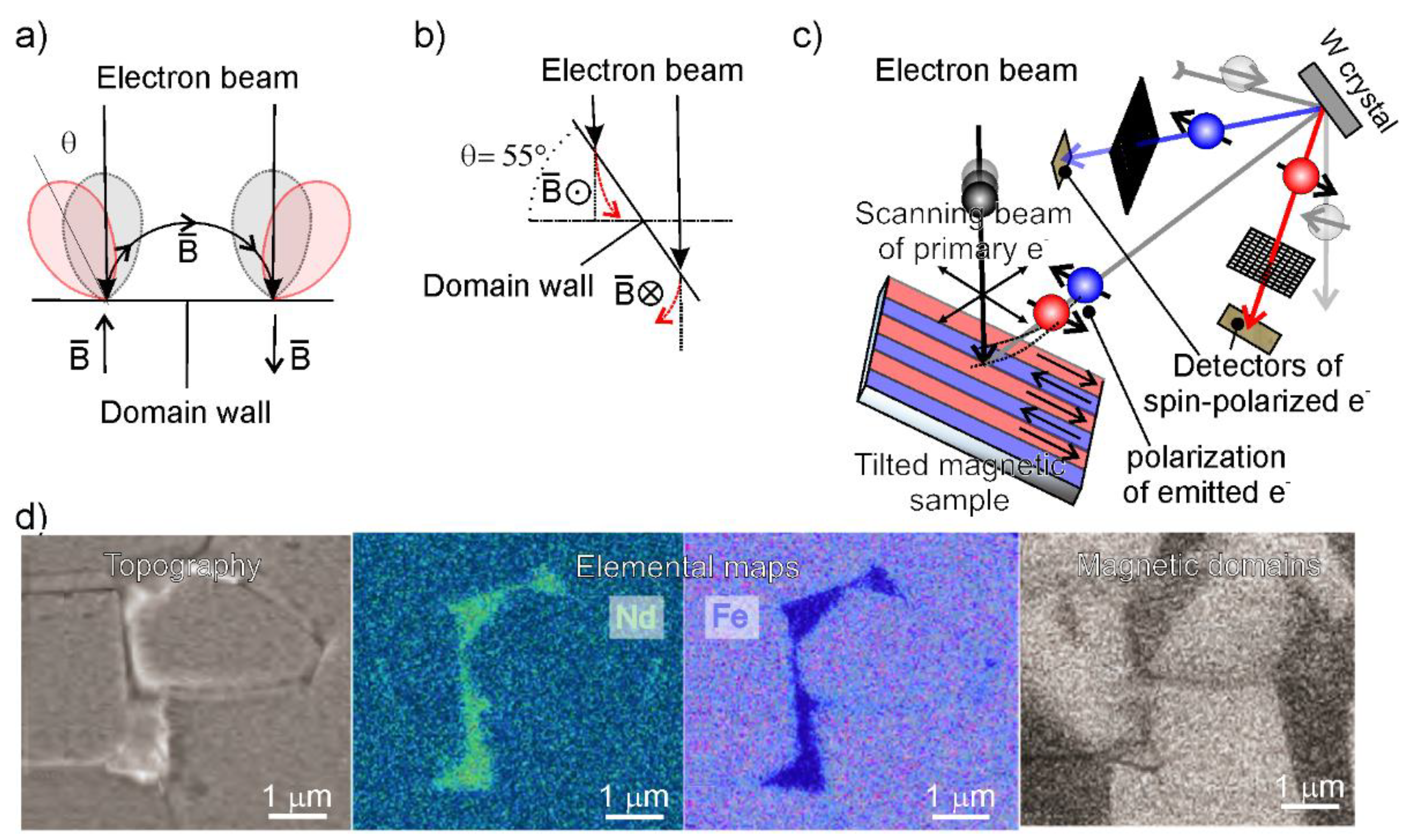
3.3. Scanning Electron Microscopy (SEM): Type-I, Type-II, and Type-III Magnetic Contrast-Based Methods

Scanning electron microscopy (SEM) technique combined with energy-dispersive X-ray spectroscopy (EDX) is commonly adopted for the chemical and structural analysis. When the sample is probed by a focused beam of electrons some signals can be obtained. Among all, secondary and backscattered electrons (SEs and BSEs, respectively) coming from the sample are collected. BSEs have energies close to that of the primary beam and give rise to a chemical contrast that is proportional to the Z of elements, while SEs are more sensitive to the topological features. Furthermore, other kinds of imaging, such as conductive and magnetic mapping [101,142], are possible.

3.3.1. Secondary Electrons (SEs), Backscattered Electrons (BSEs) Imaging

The imaging of the magnetic domain structure of a material is possible by scanning electron microscope (SEM) techniques based on the deflection of the electron beams (i.e., Lorentz force), which are exposed to a magnetic field or from the electron polarization [143]. Three different kinds of contrast mechanisms are known: Secondary electrons (SEs), backscattered electrons (BSEs), and SE polarization, known as type-I, type-II, and type-III magnetic contrast [33], firstly observed by Banbury and Nixon [144], Philibert and Tixier [145], and Pierce and Celotta [146], respectively. Nonetheless, no full description of the experimental conditions required to obtain the magnetic contrast was given and no explanation of the observed effect was described. After the first observations, the principles of the involved processes were then provided. Now it is clear that the electron deflection can be caused by the magnetic field outside (SEs) or inside (BSEs) the sample (Figure 10a,b). In both cases, no special care of the sample is required, but the surface polishing is recommended to avoid unnecessary contributions by topographic features. The main difficulty of these two techniques is related to the separation between magnetic contrast and other kinds of signals and the spatial resolution limited to the intrinsic principles of these techniques. Furthermore, the simultaneous SE and BSE-based imaging is often possible, when the two detectors are simultaneously available. While the main modification of a conventional SEM has to be dedicated to the geometry (i.e., positions of detectors) for maximizing the signal collection, the acquisition potentials should be set as low as 10 keV (i.e., maximize the emission) for SEs and as high as possible (i.e., ca. 20–200 keV) with a tilted geometric surface of about 50–55° for BSEs to obtain enough image contrast. Several studies have shown that the tilting and rotation controls are usually required to maximize the contrast for both type-I and type-II magnetic contrast imaging.

3.3.2. Scanning Electron Microscopy with Polarization Analysis (SEMPA)

The SEM with polarization analysis (SEMPA) known also as spin-polarized SEM, was first developed by Koike et al. [147] in 1984. The technique is a more advanced method for the observation of magnetic domains and is based on the spin-polarization of SE that are emitted from the local region (ca. 50 nm) of a sample surface when electrons of medium energy (10–50 keV range) probe the sample. The main difference with traditional SEM lies in the fact that electrons arrive at the sample position with a nearly zero kinetic energy. The principles of the visualization technique are based on the measurement of the spin-polarization of SEs ejected from a ferromagnetic surface after being irradiated with a high-energy electron-beam (Figure 10c). The ejected polarized electrons are detected by spin detectors allowing all three vector components of magnetization (more commonly the electron polarization along the two projected orthogonal axes parallel to the sample surface, i.e., in-plane magnetization) to be attained with a very high spatial resolution (ca. 10 nm) suitable also for 3D surfaces [116]. Spin-polarized SEM, if combined with other imaging methods currently adopted in SEM (i.e., Auger, EDX, BSE diffraction microscopy), provides insightful information on chemical elements, crystal direction and topography with an increased spatial resolution down to about 3 nm. An example is reported in Figure 10d, where a NdFeB permanent magnet is imaged. Besides magnetic domain visualization, topography and elemental distributions of Nb and Fe for the same area were obtained by scanning Auger electron microscopy by Koike [116]. By comparing the different images, the author concluded that the Nd-rich areas were found to coincide with the grain boundary regions.
A set of spin-polarized SEM characteristics merits a particular attention compared to that of other magnetic imaging techniques: (i) spin-polarized SEM directly reveals the sample magnetization, whereas the majority of imaging techniques is sensitive to the magnetic fields out/inside of the sample; (ii) the quantitative magnetic interpretation from images is possible; (iii) despite the fact that SEs are generated in large quantity and the magnetization signal is pretty high, the low efficiency of the detectors makes the measurements more problematic; (iv) a very high spatial resolution can be achieved (below 10 nm); (v) both, magnetization and SE intensity properties, can be simultaneously monitored; (vi) both, the magnetic and topographic features, can be obtained and compared, providing information on the characteristics of the magnetic domain structure.
Lastly, spin-polarization SEM signal, that is essentially sensitive to topmost few-layers, can be rapidly attenuated by the presence of non-magnetic coatings, overlays, molecularly adsorbed species, thus ion-beam together with ultra-high vacuum conditions, are gainfully required. Surface preparation under ultra-high vacuum conditions is necessary. Surfaces for spin-polarized SEM imaging can be prepared by depositing an ultra-thin overlayer of high spin polarized material (e.g., Fe). It is so assumed that, due to the very thin film thickness, the magnetic character of the underlaying sample is not significantly affected.
Depending on the emitted electrons, a lateral resolution as low as 10–50 nm can be obtained, without any contribution of the sample topography. However, the probing depth that corresponds to the quick escaping depth of SE, is of the order of a few nanometers. The typical image acquisition time depends on the image size and it is in the 1–100 min interval. SEMPA offers a series of advantages, including both the large field depth and the easily variable magnification, allowing to raster regions from a few millimeters to a few hundred nanometers. On the contrary, conductive samples are required to prevent charging effects and stray magnetic fields (above 10 Oe) must be avoided.
In recent experiments it was found that excited electrons in SEM could escape from the tip-target junction, helping in building new electronic systems based on polarized spin at nanoscale. Bertolini and co-authors [148] reported for the first time the scanning field emission microscopy with polarization analysis (SFEMPA). In SFEMPA a STM tip is held on one side and the spin polarization generated by electron scattering, thus providing the entire magnetic detail. However, due to the low efficiency of a spin polarimeter, spin-polarized images have been demonstrated to be limited to fewer pixels of the STM images during the imaging of Fe dots deposited on a W(110)-single crystal surface. The 1 nm spatial resolution, which primarily depends on the distance between the pixels, can be improved by increasing the efficiency of the spin polarimeter and by optimizing the electron optical parameters.

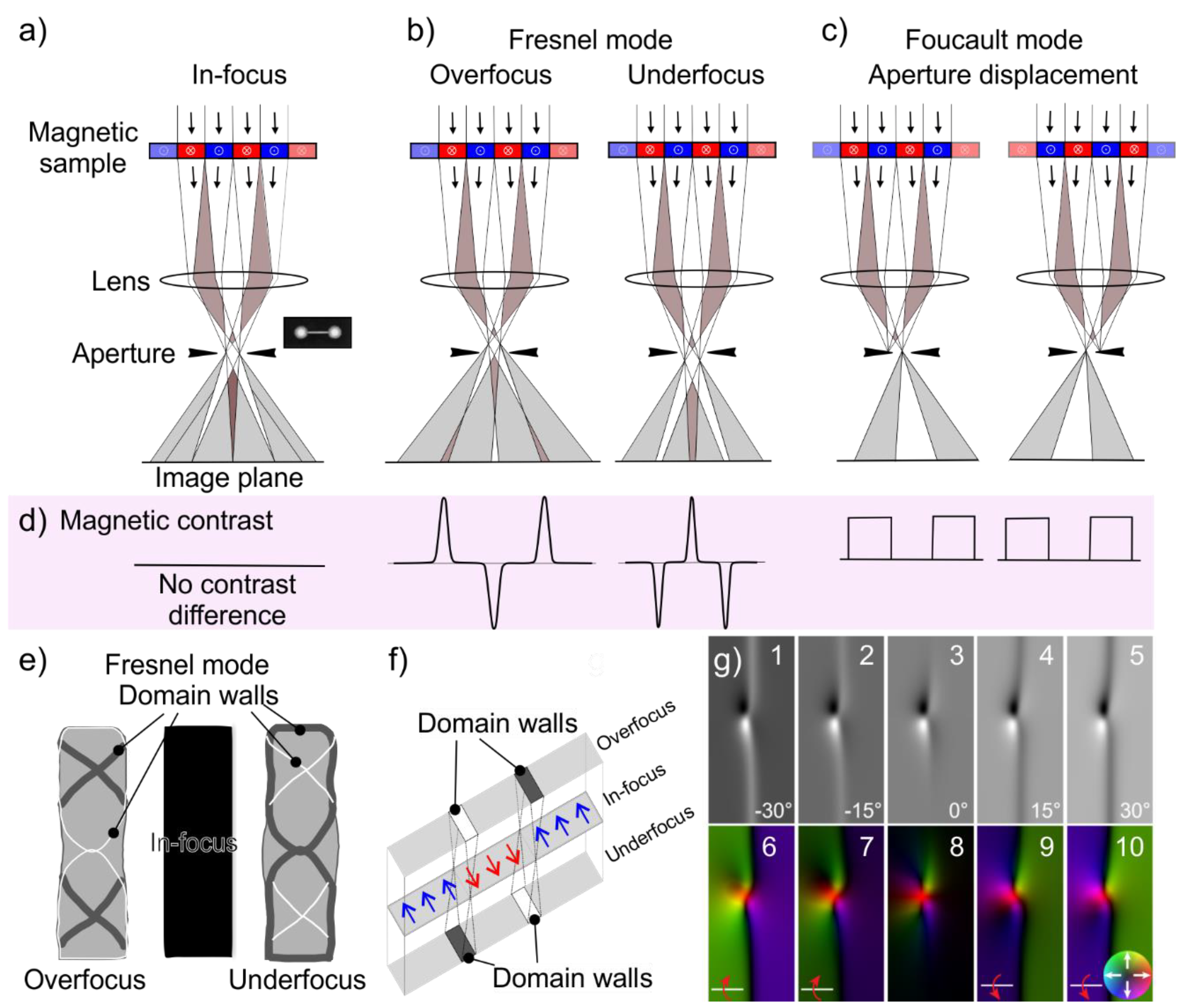
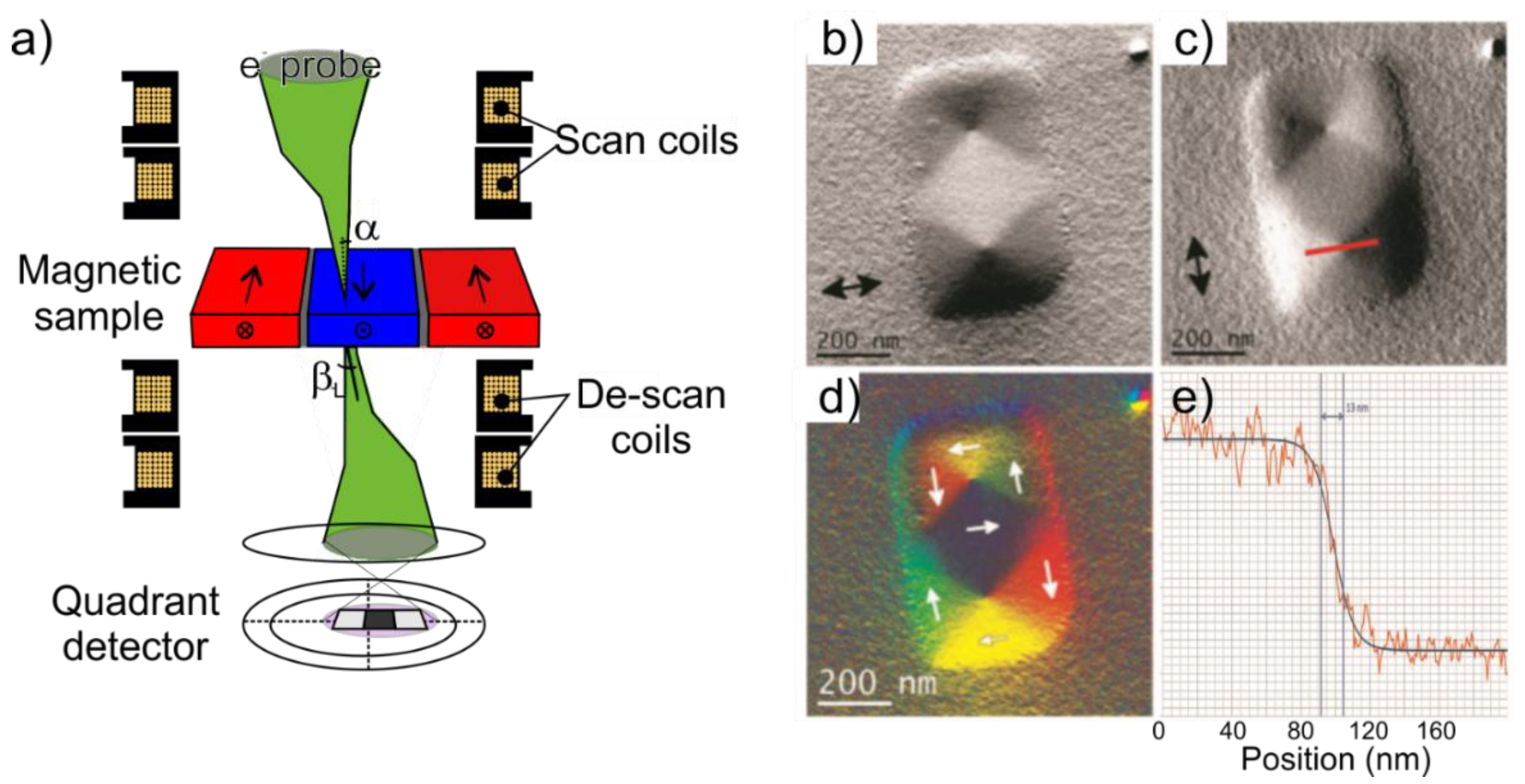
3.4. Transmission Electron Microscopy (TEM)

In the past, the spatial resolution of the TEM instruments has been primarily limited by the performances of the magnetic objective lens (and not by the incident electrons wavelength). Both, the primary image and diffraction pattern, which are responsible for the ultimate image quality, are by far affected by the lens aberration characteristics first, and are later magnified by all the other lenses. Magnetic objective lenses designed with small aberration coefficients (i.e., Cs: spherical and Cc: chromatic aberrations, respectively) for achieving atomic-scale spatial resolutions have been one primary achievement in the modern electron microscopy. Recent TEMs operate with high-power, high-quality magnetic lenses to produce magnified images. In order to obtain a short focal length, which is an essential condition to achieve atomic-resolution imaging, a relatively strong magnetic field as high as about 2–3 T is usually required inside the magnetic objective lens, where samples are placed. However, under these conditions, the magnetic and physical structures can be largely altered or even destroyed. The question can be unraveled by using newly developed magnetic objective lenses causing a magnetic field-free condition at the sample position [149]. This technical advancement, combined with the high-order aberration correction, permits to achieve a sub-angstrom spatial resolution (ca. 0.4 Å at 300 kV as an acceleration potential) [150] even under a very small residual magnetic field (below 0.2 mT) at the sample position. The direct atom-resolved imaging of magnetic materials can be attained enabling a new stage in atomic resolution electron microscopy with no alteration by high magnetic fields. In more detail, the standard double-tilt sample holders together with the interaction of the high energy beam with the sample result in characteristic spectroscopies, including electron energy loss spectroscopy (EELS) and energy dispersive X-ray (EDX) spectroscopy, which are both very informative about chemical bonds, structures, and compositions at the nanoscale. In the field of materials science, a multi-technique approach is often adopted by combining microscopies and spectroscopies together with other techniques. In this regard, the electron microscopies are more commonly used to determine the morphology and the structure, while the magnetic properties are revealed by complementary techniques [91,96,108,151].

3.4.1. Lorentz Transmission Electron Microscopies: Fresnel, Foucault and Differential Phase Contrast (DPC) Imaging

The Lorentz transmission electron microscopy (LTEM) is based on the Lorentz force causing the deflection of the electron paths of a beam perpendicularly oriented to the magnetic field. Lorentz microscopy operates in a conventional TEM or in a scanning TEM (STEM) instrument through a thin sample by means of three different techniques of imaging identified as Fresnel, Foucault (Figure 11) and differential phase contrast (DPC) microscopy (Figure 12). Lorentz microscopy in Fresnel mode (Figure 11a–d) is by far the most widely used also because the defocused electron beam transmitted through the sample is informative of the magnetic properties via the magnetic contrast located at the position of the domain walls (Figure 11d). Depending on the direction of magnetization of each domain, the beam is slightly deflected toward one or the other wall by the Lorentz force. Therefore, the domain, delimited between one bright and one adjacent dark region corresponding to the wall positions, can be visualized (Figure 11e,f). On the other hand, the domain structure in the Foucault mode is imaged in focus and the electrons, deflected by the magnetic field in one way, can be blocked by the aperture displacing (Figure 11c). The resulting contrast within a single domain thus depends on the direction of its magnetization. In both operational conditions, images directly display the domain wall structure and the dimensions can be determined quantitatively from these images.
The maximum resolution attainable for imaging the magnetic structure largely depends on several factors, including the sample type, the delocalization value of the Lorentz lens, the spherical aberration of the instrument, and it is typically in the 2–20 nm range. As far as the sample is concerned, only thin specimens (less than about 150 nm) can be analyzed. In other words, the deflection is caused by the magnetic field within the sample and the information depth comes from the full thickness of the sample and with the same weighting for all depths. TEM instruments for this appropriate practice are already available, nevertheless, the moderately high complexity of methods, together with the preparation of thin samples that may affect the domain structure, have to be considered for this kind of imaging techniques. As experimental Lorentz TEM images in Fresnel-mode do not provide a direct information regarding the magnetic induction directions, the reconstruction of the phase is typically adopted using the transport of intensity equation (TIE). Such equation when applied to a focal series of the Fresnel images, may allow in reconstructing the magnetic phase shift of the electron wave (i.e., in-plane magnetic induction properties) and the quantitative mapping of the magnetic induction is also possible. In a recent paper by Cheng et al. [152], the Fresnel mode L-TEM was used to image a DW skyrmion, a kind of topological magnetic excitation that is characterized by vortex-like magnetic structure (a distinctive 360° transition) formed by the magnetic moments of electron spins. The sample tilting procedure was performed to allow magnetic contrast to be displayed in Fresnel mode (i.e., in the absence of the tilting stage, Néel walls do not appear) and the in-the-plane magnetic component emerges from the perpendicular induction of neighboring domains giving rise to contrast at the positions of Néel walls. TIE equation is also employed to calculate the integrated in-plane magnetic induction.
Differential phase contrast (DPC) microscopy is a scanning TEM-based technique rastering athwart the specimen (Figure 12a). The local Lorentz deflection is obtained at the electron probe position and observed by utilizing a quadrant detector able to record signals from detector segments located in opposite positions, thus providing the two components of the Lorentz deflection angle (βL). Semi-quantitative maps of the magnetization directions and on the domain wall structures with a spatial resolution nearly equal to the size of the electron probe or 10–20 nm for more typical applications can be obtained. In this domain, with the aberration corrected TEM technique utilized in field-free Lorentz STEM imaging of magnetic specimens a spatial resolution lower than 1 nm for direct imaging of magnetic structure by EM is possible [153,154]. One example of the aberration corrected L-STEM is shown in Figure 12b–e. In these images a Fe60O30C10 ferromagnetic nanostructure, 50 × 500 nm in size, is imaged. The in-plane magnetic characteristics of this nanostructure show a dual vortex structure (i.e., a close loop of the in-plane induction direction). From this image it is clear that the extent of the vortex core size can be easily measured across the vortex core direction and the associated deflection angle (±25 μrad) can be assumed proportional to the integrated magnetic induction (±40 T nm) [153].

3.4.2. Electron Holography

The principles of the phase and of the electron shifts are used in the electron holography (EH) (Figure 13).
Several types of EH are known, including TEM and scanning TEM. The most used form is the off-axis electron holography that involves an electron biprism inserted in the aperture plane of the column of the microscope perpendicularly to the electron beam direction. A field emission gun (FEG) is mandatory for delivering a coherent source of electrons. Moreover, by applying a voltage to the biprism, two trajectories of electrons are found in the back focal plane to constitute the electron hologram. By increasing the biprism voltage, the electron sources are pushed further apart, which will increase the width of the hologram and decrease the fringe spacing [155]. Several studies have shown that for medium-resolution EH, alternatively to the conventional objective lens, a Lorentz lens can be used to provide a useful field of view in the range 200 nm to 2 µm.
The off-axis electron holography approach makes possible both, the direct magnetic domain imaging and quantitative measurements of the magnetic flux (B).
For these reasons, together with the high energy required (i.e., 200 keV) an interference pattern is formed from electrons in TEMs allowing to play with electron holography. When electron holography is attained for the magnetic domain imaging, an interference pattern is generated by the splitting of the beam into two components through the negatively biased electron biprism: One electron trajectory passing through the thin specimen and another being unperturbed. When the two components are recombined on the detector plane, an interference figure is thus obtained (Figure 13a). Furthermore, the obtained additional phase shift is immediately related to the total magnetic flux enclosed by the two paths of electrons. Interestingly, interference pattern lines could be immediately interpreted as the magnetic flux lines. Additionally, a procedure can also be adopted as an alternative. In other words, as both electron trajectories pass through the magnetic sample with somewhat different paths, the observed difference in phase is proportional to the flux within the dual beam regions, but it is sensitive to the domain walls. Different approaches may be tackled for extracting the shift of the phase signal related to the magnetically inducted electron wave, which is neighboring the sample. The magnetic figure can be fully quantitatively understood enabling the reconstruction of the electrostatic and magnetic phase shifts. In a paper by Serrano-Ramon et al. [156] an example of the off-axis electron holography is provided (Figure 13b–e). In the images, a 9 × 30 nm Co nanowire is illustrated together with electrostatic and magnetic phase shifts. In another paper, Almeida et al. [157] reported the magnetic structure of vortex-state Fe3O4 grains (Figure 13f–k). In these images, from the EH image (Figure 13f) by tilting the sample of equivalent and opposite angles in the ±30°–75° range (Figure 13g) the magnetic contribution was separated from the phase shift (Figure 13h). A cosine image (Figure 13i) of a chosen integer multiplied by the magnetic contribution to the phase shift shown in Figure 13j was used to generate the magnetic phase outlines (Figure 13k) within the Fe3O4 grain from the surrounding stray magnetic field. In fact, from electron holograms recorded with the particles magnetized in opposite directions, the mean inner potential (MIP) contribution to the phase could be subtracted from the total recorded phase to gain the magnetic contribution to the phase.
A spatial resolution of 10 nm is possible with electron holography with specimens about 50 nm in thickness, but thicker samples (below 150 nm) even conductive can be investigated. In any case, this technique should be intended as extremely powerful, but complex, due to the wide range of applications and difficulties in the preparation of specimens, image reconstruction and analysis time.

3.5. Spin-Polarized Low Energy Electron Microscopy (SPLEEM)

The SPLEEM has been used to address phenomena such as domain wall structures in thin magnetic films, micromagnetic configurations in surface supported nanostructures, spin reorientation transition, magnetic coupling in multilayers, phase transitions and finite-size effects. Its application has several advantages, such as real-time observation and the possibility to combine crystallography with magnetic information. The surface sensitivity limits its usefulness to samples prepared in situ (or grown elsewhere) and protected by a removable capping layer. The main disadvantage in the use of SPLEEM is its strong sensitivity to applied magnetic fields, which distress the trajectory of electrons and degrade the image quality. Modest fields of a few hundred gauss can be applied only in the surface normal direction, so that the Lorentz force is geometrically minimized. This limitation affects important fields of research, such as dynamics on domain walls and exotic magnetic states of matter. The usual image contrast is augmented by magnetic contrast generated by the exchange interaction between incident spin-polarized electrons and spin-polarized electrons in the magnetic material [95]. An important family of applications of SPLEEM employs the vector imaging capability to resolve domain wall (DW) spin textures. Zhou et al. [158] have recently reported a series of thin films, including Co/W(110), Co/Cu(001) and (Co/Ni)/W(110), obtained at zero contrast between magnetic domains. Under these conditions, the authors observed the appearance of magnetic contrast outlining the DWs.

3.6. Scanning Probe Techniques

In scanning probe methods, a sharp tip laterally scans over the sample surface. The interaction region and the resolution are primarily determined by the sizes and the properties of the tip. A feedback loop is commonly used to correct the height position of the tip and measures the tip-sample interaction. Depending on the type of the tip and sample characteristics, different scanning probe methods can be distinguished. Atomic force microscopy (AFM), takes advantage from either repulsive (contact-AFM mode) or attractive (non-contact AFM mode) interactions between the tip and the sample. The van der Waals forces are so used to regulate the tip-sample distance for the imaging from the microscale to the atomic resolution [159]. Scanning tunneling microscopy (STM) technique is based on the tunnel current between the tip and a conducting sample. The extent of the tunneling current represents the tip-sample interaction. Both AFM and STM are by far among the imaging techniques with the best lateral resolution able to detect the structure variations (i.e., conformation, adsorption geometry, bond-order relations) and visualize the charging state, when single electrons are added to or removed from small molecules (e.g., pentacene, porphine, azobenzene) or with ionic state variations from neutral to anionic and dianionic states of tetracyanoquinodimethane [160].

3.6.1. Magnetic Force Microscopy (MFM)

Magnetic force microscopy (MFM) is a relatively young technique, firstly demonstrated in 1987, but now is by far one of the most diffused investigation techniques for studying the magnetic structure at the mesoscale [161]. This technique is based on magnetic forces acting between a sharp ferromagnetic tip probe and the magnetic characteristics of a sample surface (Figure 14a,b). When the magnetic tip scans a magnetic surface, the small attraction (or repulsion) forces acting between the tip and surface are detected, thus making possible to image magnetic characteristics of the sample surface. The tip radius of 20–40 nm is used, which determines the limit of lateral resolution in the magnetic imaging.
In the typical MFM technique one (i.e., single-pass mode) or two consecutive scans (i.e., dual-pass mode) are involved. While in the single-pass mode both topography and magnetic properties are simultaneously acquired, in the dual-pass mode the topography of the surface is acquired first, by taking advantage of the van der Waals forces (i.e., short-range interactions) acting between the probe and surface, by using the conventional tapping-mode atomic force microscopy (AFM). Then, in a second scan, the probe preventively magnetized by a permanent magnet, is lifted above the surface and repeats the scanning of the surface at a constant lift height at a distance where van der Waals contributions are negligible and the magnetic tip probes are exposed only to the magnetic interactions (i.e., long-range forces). Magnetic force microscopy usually works in AC mode, in which the tip oscillates at a certain frequency near to its resonance frequency (ω0). Importantly, ω0 shifts when a force is applied on the cantilever, thus the resonance frequency shift (∆ω) depends on the force gradient, causing a variation in the phase and amplitude (Figure 14c,d, respectively).
Two key advantages of MFM are the high spatial resolution that is of the order of 40–50 nm, and the flexibility to work in environmental conditions and with applied magnetic fields. Single magnetic nanoparticles acquired in the air are shown in Figure 14e–g [65]. The chitosan-pyrolized magnetic nanoparticles (Fe3O4, γ-Fe2O3) preventively separated by a permanent magnet and deposited on a freshly cleaved mica surface were AFM imaged in a first scan (Figure 14e) and their sizes determined in the 22–30 nm range from the related height profiles.
The phase shift signal, imaged in the second scan by using the same tip probe operating in lift mode at four selected heights (90, 100, 110, 120 nm), was found to be effective in minimizing the topographic features (i.e., short-range interactions) and in revealing the magnetic characteristics (i.e., long-range forces). It is worth mentioning that negative phase shifting (darker regions in Figure 14f), depends on the operating distance and it is associated with attractive interactions between the sample and the magnetic probe in combination with a positive shift of the amplitude signal in both forward and backward scans (Figure 14g). The method is relatively simple for bulk materials, films or for nanoparticles when they are placed on flat supports, like mica or highly oriented pyrolytic graphite (HOPG). The acquisition could be much more difficult for nanoparticles dispersed into a porous carbon texture [162] or in a polymer phase [163,164]. Other key advantages offered by the technique are the possibility to work under vacuum, with or without externally applied magnetical and electrical fields and variable temperature conditions. High-resolution MFM imaging can be obtained in vacuum conditions (10−4 Pa) to benefit from higher sensitivity (i.e., higher Q factor of the cantilever) and the (thermal) stability.
In a recent paper, Geng et al. [166] showed that the magnetoelectric force microscopy (MeFM) that is a combination of magnetic force microscopy (MFM) with in situ modulated electric fields (E), can be employed to detect the E-induced magnetization (ME) and to show the multiferroic domain structure in hexagonal (h-)ErMnO3. Along with multiferroic materials (e.g., Cu2OSeO3) [167], they exhibit the so-called magnetoelectric effect, in which an external magnetic field can cause electric polarization and an electric field can cause magnetic ordering. The field of the manipulation of magnetic structures by electrical fields is beyond the scope of this review, but it is highly desirable for technological applications.
The interplay between superconductivity and magnetism in single crystal EuFe2(As0.79P0.21)2 magnetic force microscopy (MFM) operated at low temperature and without applied magnetic field has been recently reported by Stolyarov and co-authors [165]. The MFM phase shift maps (Figure 14h,i,l) are representative of three temperature regions: TFM ≲ T < Tc, T ≲ TFM < Tc, and T < TFM < Tc (in which TFM and Tc represent the ferromagnetic transition and the critical temperatures, respectively). Above TFM (ca. 18.28 K), as expected for a superconductor, the conventional Meissner state was found homogeneous (Figure 14h). Below TFM (ca. 18.23 K), the Meissner state first became striped with the domain width in the 100–200 nm range (Figure 14i), then a new phase exhibiting domain vortex-antivortex state (DVS), made of larger domains of ca. 350 nm, 40 times stronger than the magnetic contrast, was observed (Figure 14j).
The indirect magnetic force microscopy (ID-MFM) has been recently reported by Sifford et al. [108] as a novel method for the detection of magnetic domains. The newly developed method has been demonstrated for superparamagnetic iron oxide nanoparticles (SPIONs) immobilized on silicon nitride TEM windows and it has the potential to be applied in cells and tissue sections, without contaminating the magnetic probe.
Notably, due to the possible mutual interaction between tip and sample, the interpretation of MFM images is a debated topic and only qualitative data restricted to the more classical ferromagnetic samples (i.e., bulk materials, thin films, or nanostructures) are available.

3.6.2. Spin Polarized Scanning Tunneling Microscopy (SP-STM)

The spin-polarized scanning tunneling microscopy (SP-STM) is a special application of the STM technique that can provide an insightful detail of magnetic characteristics at the subatomic scale in addition to the topographic signal that is usually obtained by STM. Domain walls in antiferromagnetic/ferromagnetic systems obtained under static or dynamic magnetic and thermal conditions can be precisely determined by this technique. A magnetic-coated sharp tip scans over a sample surface under a potential applied between, thus promoting electrons to tunnel between the tip and sample and resulting in an electrical current. When the tip is magnetized the electrons having the same spin orientations (i.e., parallel orientation) at the sample surface provide a higher tunneling current than that given by spin with the antiparallel orientation (Figure 15a,b), while in the absence of magnetic interaction this current is indicative of the local electronic properties.
The magnetic probe is the most important component for the atomic spatial resolution: Both the geometry and the magnetic properties of the atomically shaped probe are crucial for the good interaction (i.e., high spin polarization, relatively small stray magnetic field and spin orientation properties at the tip apex). Three operational modes can be adopted: (i) constant current, (ii) spectroscopy, or modulated tip magnetization (exclusive for SP-STM). A particular sample (and probe) preparation is required as well as ultra-high vacuum (UHV) conditions to prevent oxidization and mislay of magnetization at the sample/tip surfaces. The separation of the magnetic features from topographic and electronic features is required also selecting the most proper operational mode.
The field of molecular magnets has become extremely active since 1990s, when it was shown that transition metal coordination molecules (i.e., [Mn12O12(OAc)16(H2O)4] (Mn12Ac) compounds) can retain magnetization for long time in the absence of external magnetic fields at liquid-helium temperatures. Over the past years, a large family of single-molecule magnets have been reported as well reviewed by Woodruff [51] and Guo [168]. In a recent paper [169], a single-molecule magnet, a dysprosium metallocene cation [(CpiPr5)Dy(Cp*)]+ (CpiPr5: penta-iso-propylcyclopentadienyl; Cp*: pentamethylcyclopentadienyl) that displays magnetic hysteresis above liquid-nitrogen temperatures, has been reported for the first time. An example of SP-STM imaging down to single molecule magnet is shown in Figure 15c–e. In a paper by Iacovita et al. [170] reported the spin polarization parallel and antiparallel of Co phtalocianine laying on magnetic nanolead support by adopting −0.32 V and −0.16 V as working potentials, respectively. A spatially resolved molecule is illustrated together with the molecular structure model superimposed (Figure 15e). In a more recent paper, Schwobel and co-authors [171] reported an atomically resolved single molecule imaged by SP-STM technique (Figure 15f,g). In these images, topographies (Figure 15f,g top panels) and spin-resolved differential conductance maps (Figure 15f,g bottom panels) of bis(phthalo cyaninato)terbium(III) (TbPc2) are shown. The topographic images showed only a slight difference, while the spin-resolved maps of differential conductance, taken with parallel or antiparallel alignments by applying a potential of −0.5 V, showed a remarkable magnetic contrast corresponding to an eight-lobe or a cross-shaped structure for parallel or antiparallel alignments, respectively. It is worth mentioning that either parallel (blue/dark colors) or antiparallel (red/grey colors) orientations can be obtained by applying an external magnetic field (B = ±1 T) and that Co islands did not rotate their orientations due to the hard magnet characteristics of Co.

3.6.3. Scanning-SQUID Microscopy

The scanning-superconducting quantum interference device (SQUID) microscopy is an ultra-sensitive technique for quantitative measurement of weak and local magnetic fields at the mesoscale. The probe, consisting of a superconducting quantum interference device (SQUID) (vide supra), allows the spatial scanning above the sample surface of hundreds of nanometers. The principal advantage and disadvantage of the scanning-SQUID microscopy with respect to the other magnetic scanning probe microscopies are the ultimate sensitivity of magnetic fields down to the nT scale and the limited spatial resolution as low as in the submicron scale only [172], although there are some promising new approaches with much higher spatial resolution. In any case, the last developed instruments allow cryogenic SQUID measurements [173]. By using microfabricated sensors, the scanning SQUID microscopy makes it possible various studies, including the ferromagnetism in novel materials and heterostructures [174] and fractional vortex formation in p-phase shift structures showing high-Tc superconducting state [175].

3.6.4. Scanning Hall Probe Microscopy (SHPM)

The scanning Hall probe microscopy (SHPM) is a variety of SPM techniques that incorporates the accurate sample approach and positioning of STM instruments equipped with a semiconductor Hall sensor. The combination of these two characteristics permits the magnetic induction mapping over a scanned surface. Although the technique has been demonstrated for domain imaging, it was originally designed for magnetic flux measurement in superconductor materials.
The SHPM technique can be considered as an improved magnetic imaging technique for a variety of reasons. Firstly, the technique can be combined with other scanning methods such as STM, but different from other methods, a small force, with negligible influence on the magnetic structure, is applied during the Hall probe analysis. Secondly, samples do not need to be electrically conductive (except for using a STM height control system). Thirdly, measurements can be performed from cryogenic to high temperatures under ultra-high vacuum (UHV) conditions, without special care of the surface or preparation. Lastly, the magnetic field sensitivity is very high (0.1 µT–10 T range). However, SHPM users have to take under consideration some limitations and difficulties, such as when they are acquiring high-resolution scans that become difficult due to the thermal noise of extremely small hall probes and that the obtained image is affected by the scanning height. Furthermore, a minimum height of the scanning distance is possible due to the hall probe assembling. Some other characteristics are in common with the probe scanning methods, for example the fact that a large scanning area is time-consuming and the importance of protecting from electromagnetic and acoustic noises (with a Faraday cage and an anti-vibrating platform, respectively) and static charge (ionizing units).
Ghirri end co-authors [176], reported the direct magnetic measurements for monolayers of molecular nanomagnets investigated by SHPM. In the paper, the magnetic response of Cs0.7Ni[Cr(CN)6]0.9 (Prussian blue analogue) molecular structure is illustrated by studying the dependency of the magnetic images on the temperature and the applied fields. Dede et al. [177] reported three dimensional (3D) scanning Hall probe microscopy (3D-SHPM) of a magnetic patterned surface down to 700 nm as spatial resolution.

3.7. X-Ray Imaging Techniques

3.7.1. X-Ray Magnetic Circular Dichroism (XMCD) and Photoemission Electron Microscopy (X-PEEM) Techniques

The magnetic structures can be investigated at the nanoscale by means of X-ray methods. The spectroscopic and microscopic approaches can serve to identify fingerprints of the magnetic matter and quantitative information as well. Along this theme, the magnetic domain visualization with a spatial resolution of a few tens of nm, even in 3D, can be obtained with various X-ray microscopy techniques. In a recent paper [121], P. Fischer reviewed the X-ray imaging methods of the magnetic structures. The authors can largely refer to this review and references therein for the sake of completeness.
The X-ray magnetic circular dichroism (XMCD) and the X-ray photoemission electron microscopy (X-PEEM) techniques have been recently developed in synchrotron facilities offering tunable and intense radiations [118] (and references therein). In this contest, the dichroism definition is essentially associated with the polarization dependency of the absorption of X-ray photons with the magnetization orientation of the sample. The different X-rays absorption process, known as X-ray dichroism, is expected to be maximized when the material magnetization and the angular momentum of photons are antiparallelly or parallelly oriented. X-ray photons entirely transfer the angular momentum to photoelectrons (i.e., angular moment conservation during the absorption process) that are excited from a splitted spin–orbit core level. The magnetic properties are then given in a second step, when two X-ray absorption spectra (XAS) collected in a magnetic field, with the left- and right-handed circularly polarized lights, respectively, are compared. Such difference in the spectra can be informative of transitions that are too weak to be detected in conventional optical absorption spectra of the atomic site, including symmetry of the electronic levels, metal ion sites spin and orbit magnetic moments and paramagnetic properties.
In PEEM equipped with soft X-rays as excitation sources (X-PEEM), XAS and X-ray photoelectron spectroscopy (XPS) can be also implemented, thus offering a set of complementary information with a lateral resolution of the order of a few nanometers. On the other hand, an electron beam can be used as a probe as an alternative (PEEM), but samples with enough conductivity should be investigated for avoiding the surface charging and a lateral resolution of about 40 nm is expected, being the sensitivity confined to the topmost layer (i.e., 1–3 external atomic layers). The X-PEEM technique has been recently used by Kleibert et al. [178] for the direct observation of superparamagnetic and unconventional magnetization state in single 3d transition metal (i.e., Fe, Co, and Ni) nanoparticles (Figure 16a–f).
Nanoparticles were imaged by means of elemental maps obtained by collecting two images for the sample site: Firstly, an edge image was recorded with the photon energy tuned at the L3 X-ray absorption edge of the element. Secondly, a pre-edge image having the photon energy tuned a few eV below the L3 X-ray absorption edge energy was recorded. Ruiz-Gomex et al. [179] investigated single-crystal magnetite islands exhibiting spin structures in ultrathin, magnetically soft magnetite by X-ray spectromicroscopy (Figure 16g–k). In these images, the triangularly-shaped island with edges aligned along the magnetite [110] directions is shown (Figure 16g). XAS image illustrated in Figure 16h exhibits a contrast with a brighter region located at the magnetite position, as obtained by collecting spatially resolved low-energy (ca. 2 eV) SEs emitted from the sample upon X-rays irradiation with a photon energy corresponding to the L3 absorption edge of Fe. X-PEEM image shown in Figure 16i illustrates an unambiguous magnetic contrast in the magnetite island, whose hexagonal pattern in the diffraction pattern, shown in Figure 16j, is indicative of an iron oxide with a spinel structure. The difference between the XAS spectra acquired with opposite light helicities from a single domain gives the corresponding XMCD spectrum shown in Figure 16k [179].
The versatility of XMCD in providing detailed information on the electronic and magnetic structure of a wide variety of systems, including nanoparticles, molecular magnets, organometallic complexes, and crystals has been recently demonstrated [118,180].

3.7.2. Scanning and Transmission X-Ray Microscopies (TXMs)

Full-field and scanning transmission X-ray microscopy (STXM) are two techniques to obtain a microscopy image by monitoring the intensity of focused X-rays transmitted through a relatively thin specimen. Since these techniques require collimated and high-intensity X-rays, the use of X-ray microscopies has been typically limited to synchrotrons. In the scanning operational mode, the X-ray beam is reduced to a small spot size at the specimen position by a focusing lens used to focus, and the sample is raster-scanned by measuring the transmitted intensity at each point. Together with transmitted X-rays, other signals (i.e., diffracted X-rays, photoelectrons and fluorescent photons) are usually simultaneously detected to map chemical and structural properties of the specimen [121,124].
On the other hand, full-field X-ray microscopy is analogous to that of conventional microscopies and the real-space image of the illuminated specimen within the field of view is directly captured. A tiny and lithographically fabricated concentric ring structure (known as zone plate) is used to focus X-rays from the synchrotron beam, working as an objective lens for X-rays. The concentric rings of the zone plate lead to the X-ray diffraction, and the observed diffraction angles depend on the wavelength, while the focal length is proportional to the energy of X-ray photons. Furthermore, the final spatial resolution is determined by the zone plate and by the width of its outmost concentric ring. With the actual lithographic feature, a spatial resolution of 10–20 nm can be attained. The technique is fast and allows the three-dimensional imaging and the study of biological specimens, when operated at near pressure conditions [125]. The energy-resolved TXM mapping can be performed with the complement provided by the X-ray absorption near-edge structure (XANES).
Comparing to PEEM, the XMCD signal monitored by TXM differs by the facts that the transmission configuration is not sensitive to external magnetic fields and it makes possible the imaging of reversal processes of magnetization, the resolution is typically higher, but the field of view cannot be easily changed. The main difference between X-PEEM and XTXM, is that X-PEEM is a more surface dependent (penetration depth is of about 2 nm), while XTXM is a transmission method through a thicker interaction region (below 50–100 nm) [124].
The photon energy can be tuned around the absorption edge of a specific element. The spatial resolution, i.e., the focusing size of the X-rays in the soft X-ray STXM is typically 20–100 nm. It is in principle determined by the diffraction limit of the lithographically fabricated FZPs.
A newly developed scanning X-ray microscope equipped with an 8T superconducting magnet as a tool for investigating the magnetic domain structures in inhomogeneous magnetic materials with a spatial resolution of 90 nm under high magnetic fields have been recently illustrated by Kotani and co-authors [181]. The performance and features were demonstrated by magnetic domain observations of Nd–Fe–B sintered magnet.
In order to shed light on both quantitative composition and 2D/3D chemical and magnetic mapping, recent improvements in soft X-ray synchrotron-based scanning transmission microscopy have been carried out (see also Section 3.9). Images with a spatial resolution better than 5 nm, obtained by a special setup including ptychographic coherent diffraction imaging in STXM platforms [182] have been obtained, as demonstrated in proton conductive ionomer in fuel cells and magnetotactic bacteria [183]. Using hard X-ray magnetic nanotomography, Donnelly and coauthors [126] have determined the 3D magnetization configuration in soft magnetic GdCo2 microcylinders. The method, based on circular left polarized X-rays with hard-X-ray dichroic ptychography, showed a spatial resolution of about 100–130 nm. Interestingly, it was shown that the two ferrimagnet sublattices are clearly coupled antiparallel to each other.
In a recent paper, Blanco-Roldan et al. [184] reported an imaging method based on the angular dependence of the magnetic contrast in a series of high resolution transmission X-ray microscopy images. For ferromagnetic NdCo5 layers 55–120 nm in thickness and NdCo5 film covered with permalloy, the authors observed a quantitative character of the magnetization (i.e., canting angles relative to the surface plane). Furthermore, the proposed method allows identifying complex topological defects (e.g., merons or ½ skyrmions).

3.8. Neutron Magnetic Imaging Techniques

The imaging techniques driven by neutrons have been documented to be very informative for the study of the inward properties of the matter, including those that cannot be investigated by X-ray sources, such as hydrogen-rich water and organic-based systems. Thermal neutrons, often with low energy (even 10−2 eV), or fast neutrons with high energies (e.g., few MeV or above 10 MeV) can be used. The energy profile covers a wide interval depending on the dedicated facilities. Fast neutrons possess a low attenuation in the most matter, thus allowing them to be transmitted through the matter. Furthermore, some new methods of imaging make use of pulsed neutron beams based on accelerator facilities as developed also at compact accelerator-driven neutron sources, which open new applications in the field of the neutron imaging. The first instrument in the world fed by pulsed neutron sources and dedicated to the imaging was realized in Japan [128].
The most relevant elements of an NTT instrument are the neutron sources, as follows: (i) radionuclide-based spontaneous fission, (ii) low Z matrix, such as Be with α emitters (i.e., Am or Po); (iii) photoneutrons, such as D or Be with a high γ-emitter, and (iv) neutron generators from deuterium–deuterium or deuterium–tritium reactions. The other principal elements are collimators and detectors. Detectors are the most relevant constituent for the high spatial resolution: Cold neutron radiography and tomography (3D) have the higher spatial resolution: about 100 µm (1–25 s as exposure time) and about 300–500 µm (10–500 ms).
As far as the magnetic imaging is concerned, neutrons have no electric charge, allowing them to be penetrated deeply into the matter. Furthermore, neutrons have a magnetic moment, making them sensitive to magnetic fields via the Zeeman interaction. Some neutron scattering techniques based on thermal neutrons have been developed to investigate the magnetic structure, as follows: (i) Polarized small-angle neutron scattering (SANS); (ii) polarized neutron reflectometry, and polarized neutron radiography and tomography. SANS is a technique perfectly appropriated for the investigation of nanoparticles, including their internal structure via the measurement of the magnetic form factor or the magnetic interactions between magnetic nanoparticles (polarized SANS technique). Polarized neutron reflectometry is more suitable for magnetic thin films (5–100 nm in thickness) by measuring directions and the magnitude of magnetic induction in heterostructures with a depth resolution of about 2–3 nm. Polarized neutron radiography and tomography technique can be adopted for films or bulk materials for mapping the distribution of induction fields by a 2D detector. The spatial distribution of magnetic fields of bulk samples have been recently developed utilizing polarized neutrons and the technique may allow to reveal the 3D magnetic field distribution in the solid matter [129].

3.9. 3D Imaging of Magnetic Domains

Three-dimensional analysis of the domain structure in bulk materials is an important issue for understanding ultimate magnetic properties and for developing materials and devices.
While bidimensional imaging of magnetic domains on surfaces can be obtained using the aforementioned techniques, 3D visualization methods have eluded scientists for many years, due to the intrinsic problems of the more conventional imaging techniques. In these years, physicists were able to study the effect of domains on the magnetic properties of materials, but they were not able to make 3D images of domains deeply inside the matter.
In the past, the magnetism was conventionally associated with the imaging and analysis of magnetic domains in ferromagnetic systems. More recently, it has been demonstrated that the magnetic structures at the nanoscale can have a more complex magnetic texture and a deeper investigation is required. A new age in the magnetism has begun thanks to the magnetic imaging techniques addressing the challenge towards the more complex 3D magnetic textures. In this context, the magnetic X-ray transmission tomography (i.e., tomographic reconstruction method) is an excellent method for rising the challenge of this new field, capable of both, probing and 3D reconstructing the magnetic textures [185]. In fact, in recent years, some approaches for the 3D visualization the magnetic domains become available. Among these, Streubel et al. [127] have shown the 3D visualization and reconstruction of magnetic domain structures in curved magnetic thin films with tubular shape by means of full-field soft X-ray microscopy with a lateral resolution of a few tens of nm. It was shown that the 3D magnetization is obtained from a 2D projection sequence by investigating the magnetic contrast that is varying with the projection angle.
In another paper, Manke, Kardjilov and colleagues’ work [186], have 3D imaged the magnetic domains by using a new technique called Talbot-Lau neutron tomography. Due to the fact that the sample slicing to investigate the interior domains could be useless, because a new domain pattern structure related to the newly developed surface can be rearranged, the tomographic approach has been developed to identify domain walls in wedge-shaped crystals basing on the refraction of neutrons (Figure 17a).
For the image contrast a double crystal diffractometer can demonstrate that domain walls oriented almost parallel to the neutron beam direction can be visualized. The setup is based on grating-based shearing interferometer consisting of three gratings: (i) source grating (GS), is an array of slits within an absorbing Gd mask with a periodicity of 790 μm; (ii) The phase grating (GPh) with a much smaller period (7.96 μm), causes a phase shift of λ/2 between incoming and produces; (iii) an analyzer grating (GA), is an absorption grating with a period of 4 μm (~PPh/2). GA is used to detect the interference pattern. The tomographic approach has been adopted for FeSi (Fe 12.8 at % Si single crystals) magnetic sample with a cylindrical shape (Figure 18b–i) [186]. An X-ray tomographic technique, more recently developed by Suzuki et al. [187], was employed to investigate the internal magnetic domain structure in ferromagnetic samples at the microscale. The technique, based on a scanning hard X-ray nanoprobe using XMCD, allows 3D reconstruction of the magnetic vector components with a spatial resolution of 360 nm. The authors argued that the method is applicable to practical magnetic materials and can be extended to 3D visualization of the magnetic domain formation process under external magnetic fields. Very recently, Wolf et al. [188] have shown the 3D magnetic induction mapping of a layered Cu/Co nanowire after reconstruction of both the magnetic induction vector field and 3D chemical composition of the material with sub-10 nm spatial resolution using the holographic vector field electron tomography approach.

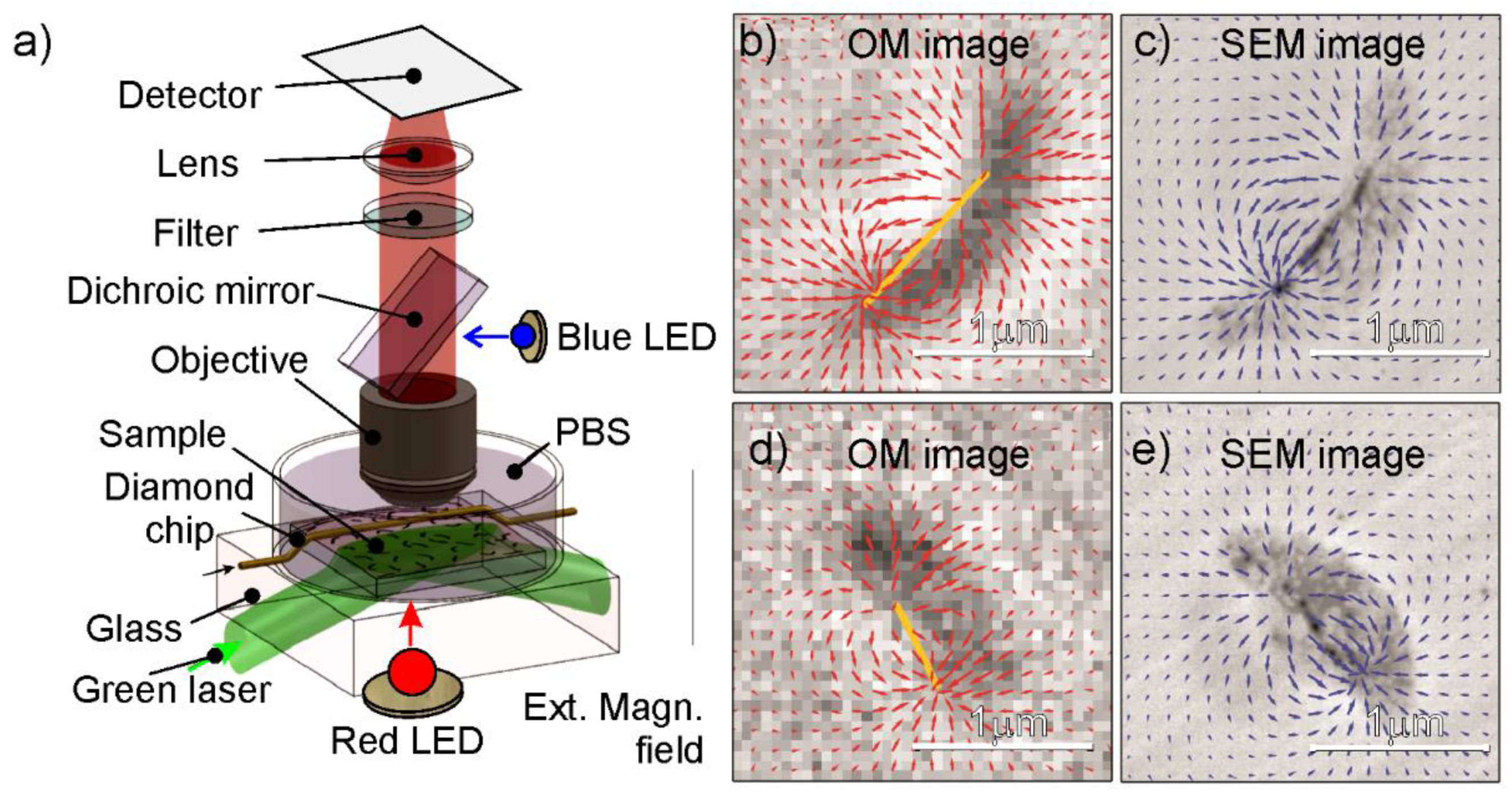
3.10. Towards Imaging in Living Matter

The development of non-invasive measurements probing magnetic fields in organisms, living matter, even down to smaller scales, possibly to single cell sizes (i.e., microns), or better, inside the cell, is a matter of great interest for the scientific community [189]. It is known that magnetic imaging methods have either low spatial resolution or they are not applicable for imaging the cell structures and living biological samples. Grinolds et al. [190] demonstrated that microscopy based on NV-center (or nitrogen–vacancy, N–V) may allow to quantitatively measure the stray field of a sample with a sensitivity down to a single electron spin. From this, the magnetic imaging of magnetotactic bacteria under ambient conditions with a nm scale resolution it was reported, using an optically detected magnetic field imaging array consisting of a N–V color centre implanted at the surface of a diamond chip (Figure 18a). Such N–V color center, absorbs the light from green and emits to the red light, thus making local magnetic field investigation possible [123]. Then, magnetotactic bacteria are placed on the diamond, and the N–V quantum spin states are optically probed, thus making possible the reconstruction of magnetic-field vector components (Figure 18b–e).
In a recent paper by Thiel et al. [191], the probing of magnetism also in 2D materials at the nanoscale with single-spin microscopy was reported. In the paper, scanning single-spin magnetometry based on diamond NV centers was used to image the magnetization, localized defects and magnetic domains of atomically thin crystals of the van der Waals magnet CrI3.

4. Characterization of Magnetic Systems for Biomedical Applications

In the previous two sections of this review, a shrewd description of a variety of representative methods currently adopted for the investigation of magnetic materials, nanoparticles and molecular structures (i.e., single-molecule magnets) is provided. In the following the authors aim at illustrating how the (inorganic) magnetic systems for biomedical uses could be designed and characterized. The field is very broad, but very relevant due to its many implications in medicine; it is difficult to summarize all methods and adopted strategies, which can be very different. Some of the most relevant techniques are discussed for the sake of brevity in the following paragraphs. It is not surprising that due to the multidisciplinarity of the fields a multi-technique approach is required to address suitable strategies to detect and monitor specific diseases in human’s body [192,193,194,195,196].
In order to evaluate potential applications of magnetic nanosystems in the biomedical field, some specific characteristics have to be carefully determined. First of all, morphology, size distribution as well as surface zeta potential must be investigated (Figure 19). Then solubility and stability in aqueous solutions have to be pursued. Possibly, relaxivity measurements could be performed to evaluate the possible application as magnetic resonance imaging (MRI) contrast agents. Finally, eventual toxicity effects exerted towards cell cultures must be assessed. In the following paragraphs some of the common techniques nowadays available to obtain precise information about magnetic systems, in view of possible biomedical applications, are enumerated and briefly discussed. For more details, the readers can refer to the more dedicated literature.

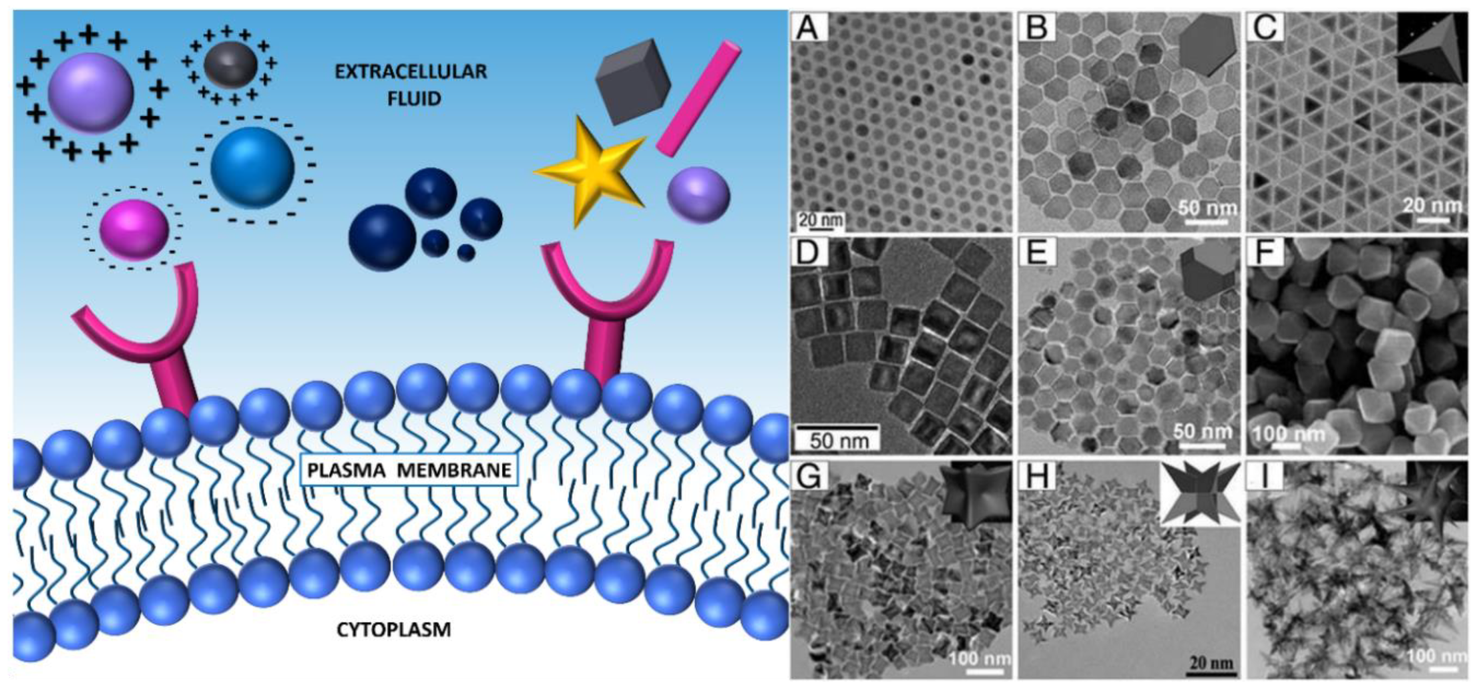
4.1. Microscopies, X-Ray Diffraction: Morphology, Composition, and Shape

Morphology and homogeneity of the sample are two fundamental aspects that should be deeply investigated in the light of in vivo administration of magnetic systems [197]. Both the morphology and the size of the system, in fact, influence its distribution, blood circulation time and possible toxicity [198,199,200]. Iron oxide nanoparticles, for instance, can be classified according to their size into USPIOs (ultrasmall superparamagnetic iron oxides), SPIOs (superparamagnetic iron oxides) or MPIOs (micrometer-sized iron oxide particles), displaying a hydrodynamic size smaller than 50 nm, about 50–150 nm or around 1 µm, respectively (coating included) [201,202]. While USPIOs are generally able to avoid the early and massive uptake by the macrophages from the mononuclear phagocyte system (especially spleen and liver macrophages), resulting in long blood circulation time and possible targeting of macrophages in deep compartments, SPIOs are generally taken up readily by macrophages in liver/spleen and provide passive targeting for reticuloendothelial system, whereas MPIOs are mostly intended to label and efficiently track macrophages [203]. Moreover, morphology and shape have been reported to affect toxicity [204]. Lee et al. [205] reported higher toxicity for rod-shaped particles in comparison to spherical ones, probably due to different wrapping mode on cell surface. Internalization through nonspecific cellular uptake was observed for rod-shaped nanoparticles more than sphere-shaped ones, resulting in faster cell penetration, dispersion throughout the cells and consequent higher pro-inflammatory cytokines production.
In order to study and report on shape and size of magnetic systems various microscopy cutting-edge techniques are employed, as reviewed in the previous paragraph. However, valid alternative and complementary methods are nowadays available [104]. Information about system structure, for instance, can be acquired by X-ray diffraction, using both conventional and synchrotron radiation sources, thermal analysis, Mössbauer [207] and infrared (IR) spectroscopy [208,209]. Conventional X-ray diffraction (XRD) is carried out to obtain information about the crystalline structure of the particles, especially about the proportion of iron oxide formed in a mixture, by comparing experimental peak and reference peak intensities [36,209]. Moreover, the crystal and particle size can also be extrapolated from the peak broadening in the XRD pattern using the Scherrer equation [104,210,211,212]. The advantage of using synchrotron radiation sources, based on a collimated light source with high intensity, instead of conventional ones, lies in the possibility of obtaining more accurate information about phase composition, crystallite size, strain and defects and of performing time-resolved studies [213]. Both types of XRD are performed on solid samples, but with energy dispersive X-ray diffraction is possible to obtain information also on samples in suspension, thus allowing knowledge of fine structural details [104,201].

4.2. Thermogravimetry and Differential Scanning Calorimetry: Thermal Properties and Composition

Another approach widely employed to the complementary characterization of magnetic systems is the thermal analysis, term that includes a group of techniques in which a physical property of a substance is measured as a function of temperature or time while the substance is subjected to a controlled temperature program. Thermal analysis provides information about sample thermal stability, adsorption of water molecules or specific coating molecules onto the magnetic core, phase transition and crystallinity of the system [214,215,216,217]. For instance, Catalano et al. [218] used thermal analysis to characterize novel hydrogel chitosan-coated iron oxide nanoparticles for cancer therapy: Through this analysis it was possible to accurately determine the chitosan content in the particle and gain information about temperature degradation of this innovative system. The most widely used thermal analysis is differential thermal analysis, DTA, in which the difference in temperature, ΔT, between the sample and a reference material is recorded while both are subjected to the same heating program. It could provide information about transformations that have occurred, such as phase transitions, crystallization, melting and sublimation. Conversely, in power-compensated differential scanning calorimetry (pc-DSC), the sample and a reference material are maintained at the same temperature; the differences in independent power supplies needed by the sample and the reference to keep this temperature constant are recorded and plotted against the programmed temperature or time [219]. Instead, thermo-gravimetric analysis (TGA), mainly exploited to determine the composition of materials and to predict their thermal stability, consists in measurements of weight/mass change (loss or gain) and the rate of weight change as a function of temperature, time and atmosphere [64,220]. An interesting example of TGA measurement applied to magnetic systems was reported by Xu and co-workers: they estimated the amount of Fe3O4 in polyacrylamide-coated magnetic particles [221]. In addition, they could correlate, with reasonable precision, the amount of magnetite with saturation magnetization, applying a specific equation. In 2014 Mansfield et al. [222] compared classical TGA with microscale-TGA (μ-TGA) in the analysis of surface coating in gold nanoparticles. They demonstrated that μ-TGA is a valid method for quantitative determination of the coatings on nanoparticles, such as surface-bond ligand coverage, and in some cases, can provide purity and compositional data of the nanoparticles themselves.

4.3. Mössbauer (or Gamma-Resonance) and Infrared Spectroscopies

Another appealing technique, probably the most adequate method to describe magnetic nanoparticle dynamics is Mössbauer (or gamma-resonance) spectroscopy [223]. Due to its relevance, Mössbauer spectroscopy should be placed among the characterization techniques dedicated to magnetic materials as well, but for the sake of brevity the technique is here briefly discussed.
Magnetic nanoparticle dynamic is related to the relaxation rates of nanoparticle magnetization vectors as determined by the size of nanoparticles. This spectroscopy method considers a group of nanoparticles as a cluster of interacting single domain magnetic particles and gives information about magnetic dipole interactions that is essential for applications involving a magnetic field such as targeted drug delivery. With Mössbauer spectroscopy three types of nuclear interactions can be typically observed: Isomer shift, quadrupole splitting and magnetic hyperfine splitting [224]. The technique is well-known due to its very high sensitivity in terms of frequency resolution, thanks to the high energy and narrow line widths of employed gamma rays. Gabbasov et al. [225] deeply characterized iron oxide nanoparticles coated with an oleic polymer using XRD and Mössbauer spectroscopy. They claimed that in some cases, X-ray diffraction measurements were unable to estimate the size of the magnetic core and Mössbauer data were necessary for the correct interpretation of the experimental results. A further example of the practical importance of Mössbauer spectroscopy in materials science is the thorough discrimination among systems having almost same structures, e.g., magnetite (Fe3O4) from maghemite (γ-Fe2O3) phase by 57Fe Mössbauer spectroscopy [96,226].
Finally, infrared spectroscopy (IR) is widely used for the complementary investigation in magnetic system characterization due to its simplicity and availability. This technique is based on the interaction between infrared radiation and matter and is extremely useful to study chemical bonds of the magnetic systems, possible surface modifications and the presence of coating molecules [227]. It can be carried out on solid samples or liquids.
However, most of the methods reported above can be employed only on dry samples, while magnetic systems for biomedical applications are usually suspended in aqueous media. To measure size and homogeneity of hydrated samples dynamic light scattering (DLS), also known as photon correlation spectroscopy (PCS), can be envisaged.

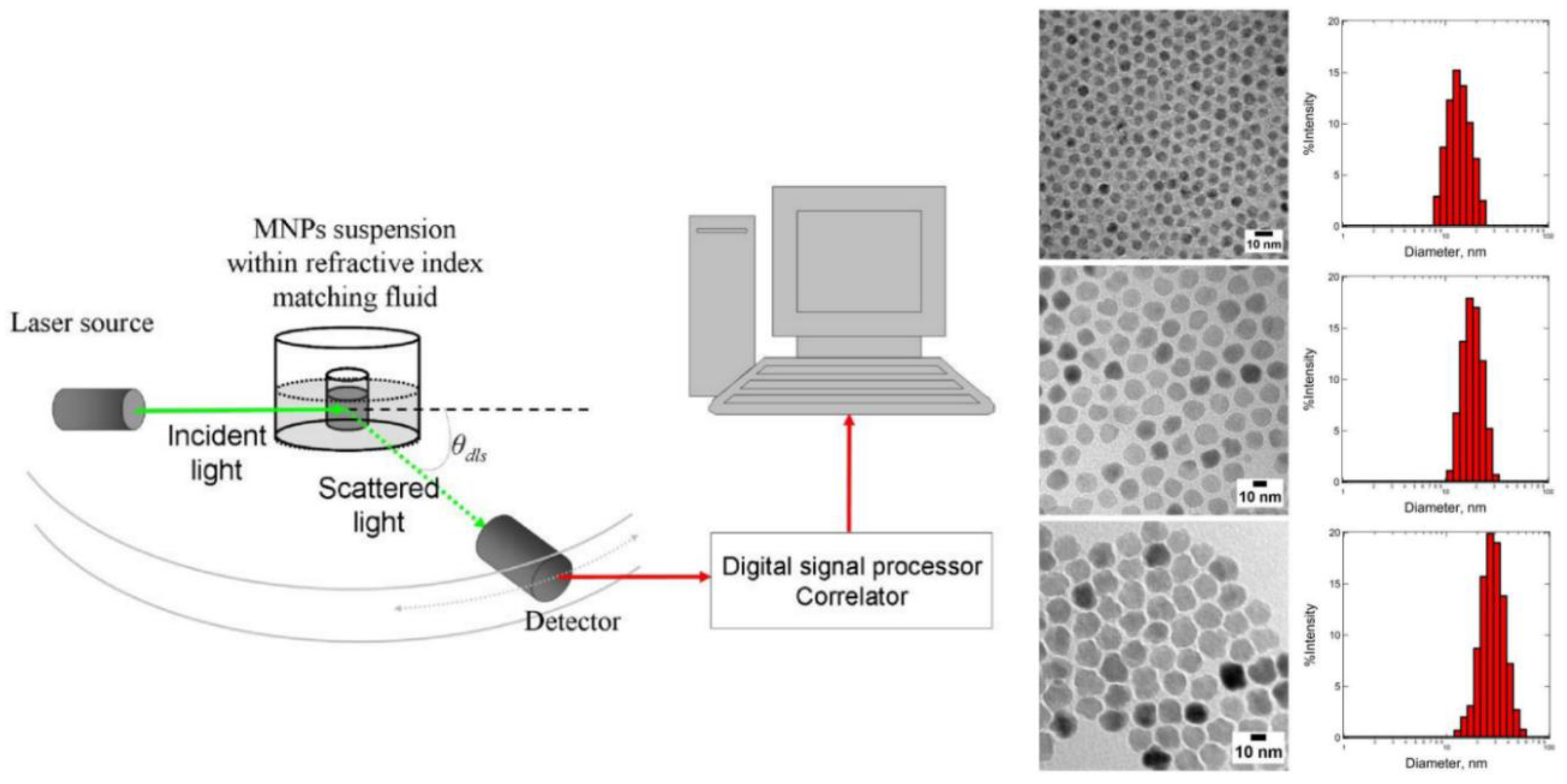
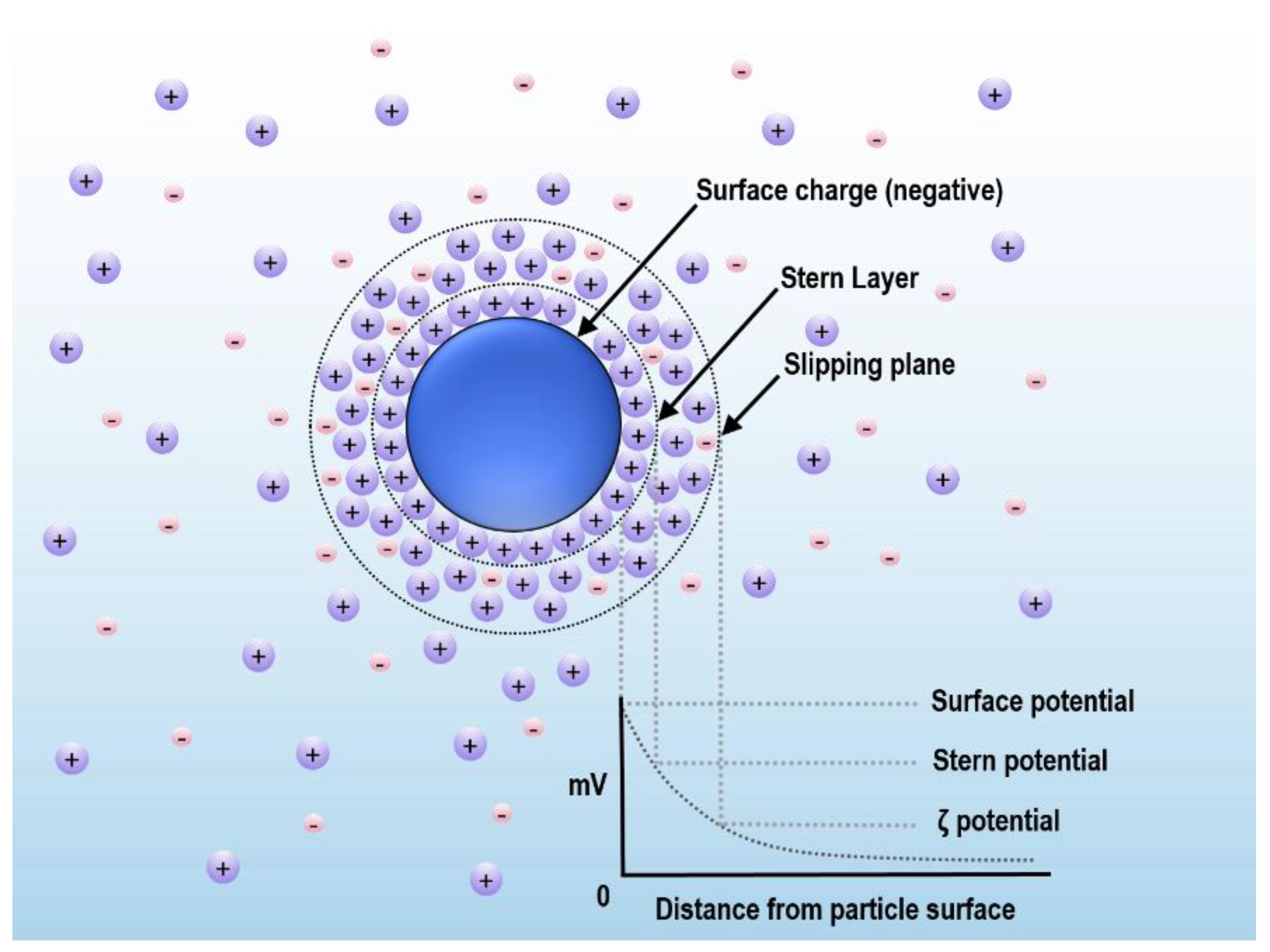
4.4. Dynamic Light Scattering and Zeta Potential: Particle Size Distribution and Particle–Liquid Interface

The employment of DLS to measure the size of magnetic nanoparticles has been already extensively reviewed by Lim et al. [228]. Briefly, during DLS measurement a light beam (electromagnetic wave) passes through a particle suspension. As the incident light impinges on the particles, a process known as scattering takes place. This process consists in alteration of the direction and intensity of the light beam. The variation of the intensity with time can then be used to measure the diffusion coefficient of the particles, that are in constant random motion (Brownian motion) due to their kinetic energy (Figure 20) [229]. Depending on the shape of the magnetic nanoparticles, for spherical particles, the hydrodynamic radius of the particle can be calculated from its diffusion coefficient by the Stokes–Einstein equation [230]. However, magnetic particle radii measured by microscopy techniques and DLS do not corroborate well. As a rule, TEM gives the “true radius” of the particle, while DLS provides the hydrodynamic radius, defined as the radius of a sphere that has the same diffusion coefficient within the same viscous environment of the particles being measured (Figure 20).
The advantage of using DLS in addition to other microscopy techniques are: (i) Wide sampling of the specimen (millions of particles), (ii) speed and ease of measurement, (iii) estimation of the radius of solvated particles (not dried and under vacuum like TEM), mimicking possible behavior in biological fluids, (iv) accessible and automated process, not requiring an extensive experience, (v) high sensitivity to the presence of small aggregates, useful to monitor sample colloidal stability [227,229,231]. The size range detectable by DLS is approximately included between 1 nm and 5 µm. The technique could also be employed to measure dimensions of non-spherical systems, such as rod-like particles, nanostars, nanotubes [232,233,234]. For example, Fang et al. [235] employed DLS to monitor the behavior of β-Ferric oxyhydroxide (β-FeOOH) nanorods depending on pH variations. They demonstrated that by DLS it was possible to monitor in situ self-assembling of this nanorods in a side-by-side fashion to form highly oriented 2D nanorod arrays which are further stacked in a face-to-face fashion to form the final 3D layered architectures. Results obtained well corroborate with TEM and SEM results. Moreover, through DLS is possible to obtain information about sample polydispersity. The polydispersity index (PDI), with 0 ≤ PDI ≤ 1, is an indicator of sample homogeneity: The lower is PDI, the higher is particle homogeneity in terms of size distribution. PDI of 0.2 and below are most commonly deemed acceptable for polymer-based nanoparticle materials [236].
Most of the instruments nowadays available to measure DLS offer the possibility to further investigate Zeta potential. Zeta potential, also known as electrokinetic potential, is the potential at the slipping/shear plane of a colloid particle moving under an electric field [229]. More in details, when a charged particle is exposed to a fluid, an electric double layer (EDL) develops on its surface. The two layers that compose the EDL are the Stern layer, which is closer to the surface, and the diffuse layer [237]. The Stern layer is primarily formed by ions/molecules with opposite charge to that of the particle, while the diffuse layer is made up of both same and opposite charged ions/molecules (Figure 21) [238]. While the charge of the Stern layer is stable as it is due to direct chemical interactions with the particle, the peculiarity of the diffuse layer is that it is dynamic as its composition is influenced by various factors (e.g., concentration, ionic strength, and pH). Zeta potential is measured at the interface between the particles, moving under the electric field, and the layer of dispersant around it.
The potential on the particle surface itself is known as the Nernst potential (ψ0) and cannot be measured [239]. Investigation of the zeta potential of magnetic nanoparticles is of utmost importance to predict their protein absorption and subsequent biological behavior, toxicity effects, possible interactions with cells and other microorganisms, as well as particle stability. Schwegmann and co-workers studied the influence of the zeta potential on the sorption between microorganisms (Saccharomyces cerevisiae and Escherichia coli) and iron oxide nanoparticles, at two different pH values, in order to evaluate potential uptake and connected toxicity effects [240]. Sharma et al. deeply investigated and compared the influence of size and charge of various magnetic particles on systemic distribution. They noticed that the highest accumulation of iron occurred in the lungs, when positively charged particles were administered, while it occurred in the liver and spleen when nanoparticles possessing a negative surface potential were injected [241]. These results suggest that nanoparticle distribution in vivo is dependent not only on the size but most likely on a complex interplay between size and charge, thus highlighting the importance of evaluating these two parameters if looking for perspective biomedical applications.

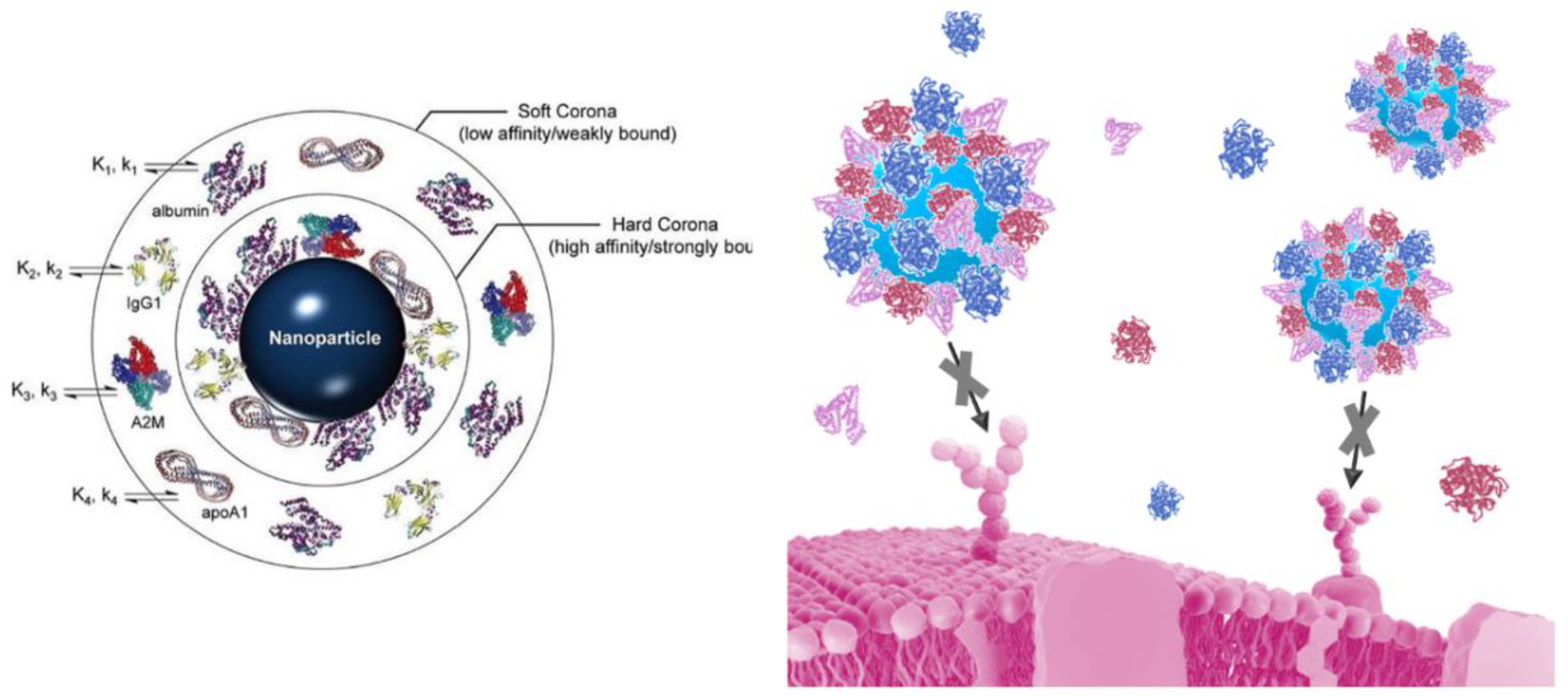
4.5. Methods to Investigate Stability and Protein Corona Adsorption

Stability of magnetic systems is of utmost importance in view of possible in vivo applications. As the colloidal stability of bare iron oxide nanoparticles, for example, is poor, different types of natural and synthetic coating materials are generally added to the preparations. Coatings can be classified into three main groups: (i) monomeric, (ii) inorganics, (iii) polymer stabilizers. Among the monomeric coating, carboxylates and phosphates are the most diffuse. Citric acid stabilized magnetic systems have been widely reported and have been also under clinical investigation [242]. Inorganic materials employed as stabilizers include silica, gold or gadolinium, leading to nanoparticles endowed with an inner iron oxide core and an outer metallic shell. As far as polymer coatings are concerned, a wide range of polymer stabilizers is nowadays available on the market, offering the possibility of tailoring each magnetic system according to its specific application. Poly(ethylenimine) (PEI), for example, is a cationic polymer frequently used to design gene-transfer vehicles for both in vitro and in vivo applications, achieving high transfection efficiency [243]. Iron oxide nanoparticles coated with the cationic polymer PEI, in fact, can easily capture negatively charged molecules, such as DNA and RNA, giving rise to cell tracking probes and MRI detectable gene/drug delivery carriers. Polyethylene glycol (PEG) is definitely the most popular coating polymer, due to its excellent anti-fouling property (preventing opsonization) and high steric hindrance, ideal to stabilize various magnetic nanoparticles. Dextran is another (bio)polymer widely used as a stabilizer, mainly because of its high biocompatibility.
In order to be administered in vivo, however, the stability of magnetic systems should be favorable not only at 4 °C in aqueous buffers, but also at 37 °C in serum or other simulated biological fluids. In the presence of serum proteins, in fact, particles can rapidly aggregate if not appropriately formulated and stabilized [244]. Moreover, the growth of protein corona onto the surface of administered magnetic systems should be investigated in order to predict their in vivo behavior [245]. Among the methods available to study particle stability there are DLS, described in the previous paragraph, which gives an idea about size variations and therefore particle aggregation and/or interaction with proteins, nuclear magnetic resonance (NMR) relaxivity studies [246], that will be described in the next paragraph and can account for particle aggregation, instability of the formulation, release of metal ions and interaction with serum proteins, such as serum albumin. TEM, SEM, AFM and fluorescence microscopy can also be used to monitor magnetic system stability [247]. Lazzari et al. [248] employed DLS to investigate the stability of various nanoparticles in buffers, simulated biological fluids (e.g., saliva, gastric juice, intestinal fluid), serum and tissue homogenates (mice brain, liver and spleen). They found out that while poly-lactic acid (PLA) particles were stable in such biologically relevant conditions, poly-methyl methacrylate (PMMA) based systems were unstable and tended to aggregate over time. Such systematic DLS studies provided an in vitro tool to investigate the stability of various systems before in vivo studies. Khan et al. [249] instead, investigated by both DLS and Zeta potential hard and soft corona formations on gold nanospheres of different sizes (2–40 nm). Understanding the dynamics of the growth of protein corona on the nanoparticle surface, indeed, is important to predict how the NPs behave in vivo. Experiments were carried out in the presence of three different proteins: Human serum albumin, bovine serum albumin, and hemoglobin. Through the correlation of obtained DLS data with mathematical modelling, they extrapolated the adsorption kinetics, number of adsorbed proteins, and binding orientation. They demonstrated that the growth kinetics of a protein corona is exclusively dependent on both protein structure and surface chemistry of the nanoparticles. In 2013, Salvati et al. [250] studied the in vivo targeting ability of transferrin-functionalized silica nanoparticles: They pointed out that due to the adsorption of protein corona onto nanoparticle surface the receptor-targeting capability was lost (Figure 22). Hence, detailed investigation to understand the effect of protein corona on different magnetic systems will enhance their translational potential and DLS can be regarded as an effective tool in such studies, along with other techniques.

4.6. Relaxometric Properties and Magnetic Fluid Hyperthermia

Amongst the possible biomedical applications of magnetic systems there are (i) separation techniques, like cell isolation and cellular proteomics [8], (ii) diagnosis, such as magnetic resonance imaging (MRI), cell tracking, biosensing, and (iii) therapy, basically including hyperthermia and drug delivery (Figure 23) [251].
In this paragraph the use of magnetic systems as MRI contrast agents or for hyperthermia mediated treatment will be discussed. To be eligible as a MRI contrast agent, the magnetic system must be superparamagnetic. Superparamagnetism is a magnetic behavior occurring in small ferrimagnetic or ferromagnetic nanoparticles. If the core diameter of these NPs is lower than 3–50 nm, depending on the material, magnetization can randomly flip direction under the influence of temperature. The mean time between two flips is called the Néel relaxation time [252]. In the absence of an external magnetic field, when the NPs magnetization measurement time is greater than the Néel relaxation time, the average value of NPs magnetization appears to be zero and these nanoparticles are said to be in the superparamagnetic state. In this state it is possible to magnetize the nanoparticles with an external magnetic field, similar to a paramagnet. However, the magnetic susceptibility of these NPs is much greater than that of paramagnets [253]. To investigate the possibility of using magnetic suspensions as MRI contrast agents longitudinal (R1) and transverse (R2) relaxivities should be measured. Relaxivity is defined as the increase of the relaxation rate of the solvent (water) induced by 1 mmol/L of the active ion. In the case of magnetite, the relaxivity is the relaxation rate enhancement observed for an aqueous solution containing 1 mmol of iron/L (Equation (2)):
R i   ( obs ) =   1 T i   ( obs ) =   1 T i   ( diam ) + r i C   i = 1   or   2
where Ri(obs) is the global relaxation rate of the aqueous system (s−1), Ti(obs) is the global relaxation time of the aqueous system (s), Ti(diam) is the relaxation time of the system before the addition of the contrast agent (s), C is the concentration of the superparamagnetic center (mmol·L−1), and ri is the relaxivity (s−1·mmol−1 L) [104]. Since relaxivity is temperature-dependent, it is usually measured at 298 K or 310 K. Superparamagnetic systems generally behave like small movable magnets, creating a strong magnetic inhomogeneity in their vicinity and considerably reducing the T2 relaxation time of nearby water protons. They are also known as signal “killers” as a negative enhancement (corresponding to image darkening) can be seen in regions in which they accumulate [254]. Recently, the use of iron oxide also as positive contrast agents, resulting in signal enhancement in regions of accumulation, has been reported by many groups [255,256]. Positive contrast agents, based on Gadolinium, are currently the mainstream clinical MRI contrast agents. However, some gadolinium-based contrast agents have shown a long-term toxicity effect (nephrogenic systemic fibrosis, NSF) and Gd depositions in the brain. On this basis, The NSF has triggered a Food and Drug Administration (FDA) black-box warning and a contraindication, as well as long term adverse effect monitoring, of some Gd-based contrast [257,258]. Newly developed ultrasmall iron oxide nanoparticles have then recently attracted much attention to serve as safer alternatives to gadolinium-based T1 contrast agents.
As a rule, to evaluate if a MRI contrast agent has higher T2 versus T1 shortening effects the ratio between the relaxivity R2 and R1 (R2/R1) must be calculated. The higher is this ratio, the higher is the predicted T2 effect. If this ratio is lower than 1, the contrast agent is predicted to be more suitable for T1 shortening purposes. Magnetic nanoparticles used in vivo are mainly composed of magnetite (Fe3O4) and maghemite (γ-Fe2O3) coated with protective shells (e.g., dextran, polyethylene glycol, starch) to prevent agglomeration. It has been reported that the coating thickness of superparamagnetic systems can significantly affect the R2, and the R2/R1 ratio. Moreover, both R1 and R2 can vary in case of system instability (metal ions release, aggregation, coating degradation) and following interactions with proteins (e.g., protein corona or specific target proteins) [259,260].
To individuate the best magnetic field at which the system can be used, the acquisition of a nuclear magnetic relaxation dispersion (NMRD) profile, which gives the evolution of the longitudinal relaxivity R1 with respect to the external magnetic field, is envisaged (Figure 24).
The model to fit NMRD experimental data, proposed by Roch et al. [261] and further developed by Gossuin et al. [262], can provide information about the nanomagnet crystals: Their average radius, their Néel relaxation time, their anisotropy energy and their specific magnetization. Combining these data with the results obtained by magnetometry is possible to obtain a very complete description of the morphology and physical properties of a magnet [261,263]. Ruggiero et al. [264] compared NMRD profiles of newly-synthesized iron oxide nanoparticles coated with Poly(lactic-co-glycolic acid) (PLGA) to the NMRD profile of Endorem™ (commercially available SPIO particles used as MRI contrast agent). From these profiles, displaying a shape of the curve typical of the relaxation induced by superparamagnetic particles, they deduced that loading iron oxide nanoparticles into the PLGA matrix seems not to affect their overall magnetic properties. Moreover, they pointed out that the different profile shapes observed for the various preparations depend on the particle properties (such as: size, clustering, Néel relaxation time and saturation magnetization) [264].
PLGA particles reported by Ruggiero et al. [264] were designed for magnetic fluid hyperthermia (MFH) applications. The use of nanomaterials for MFH was first investigated in 1957 by Gilchrist et al. [265]. The authors reported the possibility of heating various tissue samples with particles of γ-Fe2O3 (20–100 nm in size) exposed to a 1.2 MHz magnetic field. Since then, the use of different magnetic materials, particle design and delivery methods, as well as various field strengths and frequencies have been investigated for MFH purposes [266]. Briefly, when exposed to a fast switching magnetic field, the magnetization of superparamagnetic nanoparticles can quickly flip direction. The friction caused by the rotation of the particle itself, known as Brownian relaxation, and the spin fluctuations within the crystal, known as Néel relaxation, lead to the loss of magnetic energy and the generation of thermal energy [252]. The heating power of a certain magnetic system, expressed as the specific absorption rate (SAR, W/g), mainly depends on the mean size of the system, on its saturation magnetization (Ms) and magnetic anisotropy (K) as well as on the alternating magnetic field amplitude (Hmax) and frequency (f). MFH effect can be exploited in cancer treatment, to raise the temperature at the tumor site above the systemic one, or to induce a controlled drug release through the thermal stimulus [267]. This field is also known as theranostics: A discipline that combines diagnostic, as superparamagnetic nanoparticles can be used as MRI contrast agents, and localized therapy, through controlled temperature increase or drug release. For practical therapeutic applications, a temperature of 41–46 °C must be reached with hyperthermia. Temperatures greater than 50 °C cause thermoablation and can induce several side effects. Therefore, it is of crucial importance for the development of MFH dedicated systems to rely on analytical methods able to characterize new magnetic nanoparticles and to predict their heating capacity in physiological conditions. Besides NMRD profiles, that, as previously described, allow to predict magnetic systems performance in both MRI and MFH applications, other particle characteristics can account for MFH efficiency. Size, volume, and morphology of the NPs can be determined by DLS, SEM, and TEM; stability of the preparation and zeta potential should be investigated. Thermogravimetric analysis, X-ray diffraction and magnetometry can be exploited to obtain valuable additional information. Finally, heating efficiency, reported in terms of SAR, can be measured by exposing the magnetic fluid to a time varying magnetic field [268]. Therefore, all the techniques described in this last section can be exploited to fully characterize magnetic systems for MFH purpose.
Given the variety of information that can be gained with the here reported techniques, for the sake of clearness, in Table 2 a recapitulatory comparison between all the reported techniques (even if we know that the list is not exhaustive), useful to characterize magnetic materials for biomedical applications, is provided. More in details, advantages and limitations of each technique are reported, as well as the specific information that can be obtained with the different instrumentations.

4.7. Toxicity Assays

Toxicity effects exerted towards cell cultures and blood components must be investigated before testing the magnetic systems directly in vivo. Obviously, it must be taken into account that these assays can be highly operator-dependent and that the lack of standard protocols make more difficult the comparison between different systems. However, the higher is the number of tests performed, the safer can be considered the preparation. Classical and less expensive cytotoxicity tests include MTT assay, Alamar Blue and Trypan blue exclusion assay. The MTT (3-[4,5-dimethylthiazol-2-yl]-2,5 diphenyl tetrazolium bromide) colorimetric assay is based on the cleavage by mitochondrial activity of the yellow soluble tetrazolium salt, MTT, to form an insoluble dark blue formazan product. As mitochondrial activity is generally proportional to the number of viable cells, this test can be used to estimate the cytotoxic effect of various compounds in vitro. Cells are first incubated with different concentrations of the system to be tested and for different time ranges, then the system is washed away, cells are then incubated with MTT for a few hours and the presence of violet formazan can be analyzed using a plate reader. The samples must be always compared to controls to determine the percentage of viable cells. In order to obtain accurate and reliable results particular attention should be devoted to cell density, culture medium and MTT exposure time [275]. Similar to MTT, the Alamar Blue test is based on the reduction of the blue non-fluorescent dye resazurin, upon entering living cells, to resofurin, a pink-colored highly fluorescent compound. The amount of fluorescent compound produced can be quantified and correlated to the number of viable cells. Resazurin is then considered a reliable indicator of the oxidation–reduction (REDOX) processes that occur both during aerobic and anaerobic respirations in cells incubated with various molecules, systems and/or drugs [276]. The trypan blue dye exclusion test, instead, is based on the different permeability of cell membranes towards certain molecules (e.g., trypan blue, eosin or propidium): While these substances can easily penetrate in dead cells, they cannot cross the membrane of living cells. To perform this test the cells are mixed with a solution of trypan blue and then the number of blue colored cells (died cells) versus the number of cells having a clear cytoplasm (living cells) are immediately quantified by visual inspection. The percentage viable cells in incubated samples will be then compared to the percentage of viable cells in control samples. All these assays can be used not only to assess cell viability, but also cell proliferation. To this aim, after incubation with variable amounts of the magnetic system and for variable time ranges, cells are washed and incubated in culture medium for different days. The number of viable cells measured at 24, 48, and 72 h post incubation allows estimating the cell proliferation time, which is then compared to that of control cells. A biocompatible system should not affect this parameter. Other convenient assays are the metabolic NAD/NADH fluorimetric assay, the protease viability marker assay, the Comet assay, useful to quantify DNA damages induced by the preparation, and the ATP (Adenosine 5′-triphosphate) quantification test, using firefly luciferase. As each cell viability assay displays its own advantages and drawbacks the most appropriate to each situation should be selected. MTT and Alamar Blue tests for example are less expensive than the ATP detection assay. However, the ATP detection assay is characterized by fewer steps, a minimum amount of interferences and is by far the most sensitive [277].
Another assay, widely used to evaluate potential cytotoxicity of magnetic particles, is the reactive oxygen species (ROS) production test. This test is based on the use of specific kits able to detect and quantify ROS, as an indicator of cell oxidative stress. ROS include hydrogen peroxide, anions and hydroxyl radicals. The production of free radicals, challenged in cells by a “detoxification” mechanism, which involves enzymes such as superoxide dismutase and glutathione peroxidase, is considered one of the primary mechanism of nanoparticle induced toxicity. The overproduction of ROS has been associated to DNA strand breaks, alteration in gene transcription, lipid peroxidation and generation of protein radicals [278]. Incubation with various magnetic systems could also induce apoptosis, a well-controlled, tightly regulated physiological process, in which the cells participate in self-destruction. Numerous assays are nowadays available to measure the number of apoptotic cells: light microscopy (Trypan blue staining), fluorescence microscopy (acridin orange/ethidium bromide and annexin V/propidium iodide staining) and agarose gel electrophoresis of fragmented genomic DNA. Trypan blue and Hoechst staining detect apoptotic cells on the basis of their reduced DNA content and morphological changes that include nuclear condensation; annexin-V and propidium iodide can distinguish between early and late apoptotic events based on plasma membrane composition and function. The cleavage of many cellular proteins, carried out by apoptosis-activated caspases, results in fragments that can serve as apoptosis markers [279].
Finally, the hemocompatibility properties of magnetic systems can be investigated by means of a standard hemolysis test [280]. Following the incubation of animal (e.g., rabbit, mouse, rat) or human donor erythrocytes with the system, the amount of released hemoglobin is measured by means of UV–vis spectroscopy (λ = 415 nm). Released hemoglobin is directly related to the number of destroyed erythrocytes that could then be easily estimated. Normal saline and deionized water are generally used as negative (0% hemolysis) and positive (100% hemolysis) controls, respectively. The percentage hemolytic rate % HR can be calculated as (Equation (3)):
%   H R =   mean   O D   of   sample   to   be   tested     mean   O D   of   negative   control mean   O D   of   positive   control     mean   O D   of   negative   control   ×   100
where OD stands for optical density. If the hemolytic rate is less than 5%, the material will have no hemolytic effect and conform to the requirements of the hemolysis test for medical materials [281].
In Table 3 a comparison between the most diffuse toxicity assays, useful to evaluate potential toxic effects exerted by magnetic NPS, is reported.

5. Conclusions

Magnetic systems and particles are extremely appealing materials that found applications in a large variety of advanced technological fields. In the last decades, the scientific literature reported a plethora of research studies and documents characterized by different physicochemical, morphological, and biological methods (depending on the use), fundamental for pointing out their magnetic response/properties. However, due to the multidisciplinary approach proper of these studies, in most cases such very specific characterization techniques are little known (or fully unknown) to most of the users.
Therefore, in order to overcome this lack, the main goal of this review is to summaries (in a detailed, but hopefully concise manner) a large number of techniques that are currently available to characterize magnetic systems, highlighting the ordinary uses together with the main relevant advantages and disadvantages.
More in details, characterization techniques were classified into three sections, and properly discussed with examples from the literature. Part I is dedicated to the definitions of magnetism and magnetization (hysteresis) techniques. Part II is dedicated to the morphological aspects, thus illustrating all the different visualization methods of magnetic domains. Finally, Part III is dedicated to the principal physicochemical characterizations, with a last section particularly devoted to the biomedical applications.
With this review, authors hope of having provided a real toolbox that acts as guidelines for helping in the choice of the most suitable method(s) as appropriate, as well as in the comprehension of the magnetic properties/responses of these promising materials.

Author Contributions

The review was written through contributions of all authors. All authors have read and agreed to the published version of the manuscript.

Funding

This work was supported by MIUR (Ministero dell’Istruzione, dell’Università e della Ricerca), INSTM Consorzio and NIS (Nanostructured Interfaces and Surfaces) Inter-Departmental Centre of University of Torino.

Conflicts of Interest

The authors declare no conflict of interest.

Abbreviations

AFM: atomic force microscopy; ATP: Adenosine 5′-triphosphate B: magnetic flux; BSE: backscattered electrons; Cc: chromatic aberration; Cs: spherical aberration; DLS: dynamic light scattering; DPC: differential phase contrast; DTA: differential thermal analysis; DW: domain walls; ED pattern: electron diffraction pattern; EDL: electric double layer; EDX: energy dispersive X-ray; EELS: electron energy loss spectroscopy; EH: electron holography; FDA: Food and Drug Administration; FEG: field emission gun; HOPG: highly ordered pyrolytic graphite; HR: Hemolytic rate; HV: high vacuum; IR spectroscopy: Infrared spectroscopy; L-MOKE: longitudinal MOKE; LTEM: Lorentz transmission electron microscopy; MFH: magnetic fluid hyperthermia; MFM: magnetic force microscopy; MIP: mean inner potential; MOKE: magneto-optical Kerr effect; MPIOs: micrometer-sized iron oxide particles; MRI: magnetic resonance imaging; MTT: (3-[4,5-dimethylthiazol-2-yl]-2,5 diphenyl tetrazolium bromide; NMR: Nuclear magnetic resonance; NMRD: Nuclear magnetic relaxation dispersion; NPs: nanoparticles; NSF: nephrogenic systemic fibrosis; OD: optical density; pc-DSC: power-compensated differential scanning calorimetry; PCS: photon correlation spectroscopy; PDI: polydispersity index; PEEM: photoemission electron microscopy, PEG: polyethylene glycol; PEI: poly(ethylenimine) PLGA: poly(lactic-co-glycolic acid); P-MOKE: polar MOKE; R1: longitudinal relaxivity; R2: transversal relaxivity; ROS: reactive oxygen species; SAM: Auger electron microscopy; SANS: small-angle neutron scattering; SAR: specific absorption rate; SE: secondary electrons; SEM: scanning electron microscopy; SEMPA: spin-polarized analysis SEM; SHPM: scanning Hall probe microscopy; SPIOs: superparamagnetic iron oxides; SPLEEM: spin-polarized low energy electron microscopy; SPM: scanning probe microscopy; SP-STM: spin polarized scanning tunneling microscopy; SQUID: superconducting quantum interference device; STEM: scanning transmission electron microscopy; STM: scanning tunneling microscopy; T1: longitudinal relaxation time; T2: transversal relaxation time; TEM: transmission electron microscopy; TGA: thermogravimetric analysis; TIE: transport-of-intensity equation; T-MOKE: transversal MOKE; TXMCD: transverse X-ray magnetic circular dichroism; UHV: ultra-high vacuum; USPIOs: Ultrasmall superparamagnetic iron oxides; XANES: X-ray absorption near-edge structure XANES; XAS: X-ray absorption spectroscopy; XMCD: X-ray magnetic circular dichroism; XRD: X-ray diffraction.

References

  1. Nisticò, R. Magnetic materials and water treatments for a sustainable future. Res. Chem. Intermed. 2017, 43, 6911–6949. [Google Scholar] [CrossRef]
  2. Bozorth, R.M. Magnetism. Rev. Modern Phys. 1947, 19, 29–86. [Google Scholar] [CrossRef]
  3. Singh, R. Unexpected magnetism in nanomaterials. J. Magn. Magn. Mater. 2013, 346, 58–73. [Google Scholar] [CrossRef]
  4. Mehta, R.V. Synthesis of magnetic nanoparticles and their dispersions with special reference to applications in biomedicine and biotechnology. Mat. Sci. Eng. C 2017, 79, 901–916. [Google Scholar] [CrossRef]
  5. Gupta, A.K.; Gupta, M. Synthesis and surface engineering of iron oxide nanoparticles for biomedical applications. Biomaterials 2005, 26, 3995–4021. [Google Scholar] [CrossRef]
  6. Tietze, R.; Zaloga, J.; Unterweger, H.; Lyer, S.; Friedrich, R.P.; Janko, C.; Pottler, M.; Durr, S.; Alexiou, C. Magnetic nanoparticle-based drug delivery for cancer therapy. Biochem. Biophys. Res. Commun. 2015, 468, 463–470. [Google Scholar] [CrossRef]
  7. Serrà, A.; Gimeno, N.E.; Gómez, E.; Mora, M.; Sagristá, M.L.; Vallés, E. Magnetic Mesoporous nanocarriers for drug delivery with improved therapeutic efficacy. Adv. Funct. Mater. 2016, 26, 6601–6611. [Google Scholar]
  8. Kurgan, E.; Gas, P. Magnetophoretic Placement of Ferromagnetic Nanoparticles in RF Hyperthermia. In Proceedings of the 2017 Progress in Applied Electrical Engineering (PAEE), Koscielisko, Poland, 25–30 June 2017; pp. 1–4. [Google Scholar] [CrossRef]
  9. Sheng, Y.; Li, S.; Duan, Z.; Zhang, R.; Xue, J. Fluorescent magnetic nanoparticles as minimally-invasive multi-functional theranostic platform for fluorescence imaging, MRI and magnetic hyperthermia. Mater. Chem. Phys. 2018, 204, 388–396. [Google Scholar] [CrossRef]
  10. Pankhurst, Q.A.; Connolly, J.; Jones, S.K.; Dobson, J. Applications of magnetic nanoparticles in biomedicine. J. Phys. D Appl. Phys. 2003, 36, R167–R181. [Google Scholar] [CrossRef] [Green Version]
  11. Garello, F.; Vibhute, S.; Gunduz, S.; Logothetis, N.K.; Terreno, E.; Angelovski, G. Innovative design of Ca-sensitive paramagnetic liposomes results in an unprecedented increase in longitudinal relaxivity. Biomacromolecules 2016, 17, 1303–1311. [Google Scholar] [CrossRef]
  12. Liu, W.; Wong, P.K.J.; Xu, Y. Hybrid spintronic materials: Growth, structure and properties. Progr. Mater. Sci. 2019, 99, 27–105. [Google Scholar] [CrossRef]
  13. Tudu, B.; Tiwari, A. Recent developments in perpendicular magnetic anisotropy thin films for data storage applications. Vacuum 2017, 146, 329–341. [Google Scholar] [CrossRef]
  14. Peyer, K.E.; Zhang, L.; Nelson, B.J. Bio-inspired magnetic swimming microrobots for biomedical applications. Nanoscale 2013, 5, 1259–1272. [Google Scholar] [CrossRef]
  15. Li, J.; Barjuei, E.S.; Ciuti, G.; Hao, Y.; Zhang, P.; Menciassi, A.; Huang, Q.; Dario, P. Magnetically-driven medical robots: An analytical magnetic model for endoscopic capsules design. J. Magn. Magn. Mater. 2018, 452, 278–287. [Google Scholar] [CrossRef]
  16. Fu, F.; Dionysiou, D.D.; Liu, H. The use of zero-valent iron for groundwater remediation and wastewater treatment: A review. J. Hazard. Mater. 2014, 267, 194–205. [Google Scholar] [CrossRef] [PubMed]
  17. Ivanets, A.I.; Srivastava, V.; Roshchina, M.Y.; Sillanpää, M.; Prozorovich, V.G.; Pankov, V.V. Magnesium ferrite nanoparticles as a magnetic sorbent for the removal of Mn2+, Co2+, Ni2+ and Cu2+ from aqueous solution. Ceram. Int. 2018, 44, 9097–9104. [Google Scholar] [CrossRef]
  18. Nistico, R.; Cesano, F.; Franzoso, F.; Magnacca, G.; Scarano, D.; Funes, I.G.; Carlos, L.; Parolo, M.E. From biowaste to magnet-responsive materials for water remediation from polycyclic aromatic hydrocarbons. Chemosphere 2018, 202, 686–693. [Google Scholar] [CrossRef]
  19. Palma, D.; Bianco Prevot, A.; Celi, L.; Martin, M.; Fabbri, D.; Magnacca, G.; Chierotti, M.; Nisticò, R. Isolation, characterization, and environmental application of bio-based materials as auxiliaries in photocatalytic processes. Catalysts 2018, 8, 197. [Google Scholar] [CrossRef] [Green Version]
  20. Neamtu, M.; Nadejde, C.; Hodoroaba, V.D.; Schneider, R.J.; Verestiuc, L.; Panne, U. Functionalized magnetic nanoparticles: Synthesis, characterization, catalytic application and assessment of toxicity. Sci. Rep. 2018, 8, 6278. [Google Scholar] [CrossRef] [Green Version]
  21. Sun, Z.; Zhou, X.; Luo, W.; Yue, Q.; Zhang, Y.; Cheng, X.; Li, W.; Kong, B.; Deng, Y.; Zhao, D. Interfacial engineering of magnetic particles with porous shells: Towards magnetic core—Porous shell microparticles. Nano Today 2016, 11, 464–482. [Google Scholar] [CrossRef]
  22. Yermolenko, I.Y.; Ved, M.V.; Sakhnenko, N.D.; Shipkova, I.G.; Zyubanova, S.I. Nanostructured magnetic films based on iron with refractory metals. J. Magn. Magn. Mater. 2019, 475, 115–120. [Google Scholar] [CrossRef]
  23. Chen, X.-Z.; Hoop, M.; Mushtaq, F.; Siringil, E.; Hu, C.; Nelson, B.J.; Pané, S. Recent developments in magnetically driven micro- and nanorobots. Appl. Mater. Today 2017, 9, 37–48. [Google Scholar] [CrossRef] [Green Version]
  24. Bedanta, S.; Petracic, O.; Kleemann, W. Supermagnetism. In Handbook of Magnetic Materials; Bruck, E., Ed.; Elsevier: North Holland, The Netherlands, 2015; Volume 23, pp. 1–83. [Google Scholar]
  25. Karimi, Z.; Karimi, L.; Shokrollahi, H. Nano-magnetic particles used in biomedicine: Core and coating materials. Mat. Sci. Eng. C 2013, 33, 2465–2475. [Google Scholar] [CrossRef] [PubMed]
  26. Li, D.; Li, Y.; Pan, D.; Zhang, Z.; Choi, C.-J. Prospect and status of iron-based rare-earth-free permanent magnetic materials. J. Magn. Magn. Mater. 2019, 469, 535–544. [Google Scholar] [CrossRef]
  27. Rossi, L.M.; Costa, N.J.S.; Silva, F.P.; Wojcieszak, R. Magnetic nanomaterials in catalysis: Advanced catalysts for magnetic separation and beyond. Green Chem. 2014, 16, 2906–2933. [Google Scholar] [CrossRef]
  28. Sundaresan, A.; Rao, C.N.R. Ferromagnetism as a universal feature of inorganic nanoparticles. Nano Today 2009, 4, 96–106. [Google Scholar] [CrossRef]
  29. Hubert, A.; Schäfer, R. Magnetic Domains, The Analysis of Magnetic Microstructures; Springer-Verlag: Berlin/Heidelberg, Germany, 1998. [Google Scholar] [CrossRef]
  30. Tumanski, S. Handbook of Magnetic Measurements; CRC Press, Taylor & Francis Group: Boca Raton, FL, USA, 2011. [Google Scholar]
  31. Craik, D.J.; Tebble, R.S. Magnetic domains. Rep. Prog. Phys. 1961, 24, 116–166. [Google Scholar] [CrossRef]
  32. Jiles, D.C.; Atherton, D.L. Theory of ferromagnetic hysteresis. J. Magn. Magn. Mater. 1986, 61, 48–60. [Google Scholar] [CrossRef]
  33. Newbury, D.E.; Joy, D.C.; Echlin, P.; Fiori, C.E.; Goldstein, J.I. Advanced Scanning Electron Microscopy and X-Ray Microanalysis; Springer Science: New York, NY, USA, 1986. [Google Scholar] [CrossRef]
  34. Jiles, D.C. Theory of the magnetomechanical effect. J. Phys. D Appl. Phys. 1995, 28, 1537–1546. [Google Scholar] [CrossRef]
  35. Chien, C.L. Magnetism and Magnetic Measurement, Introduction. In Characterization of Materials, 2nd ed.; Kaufmann, E.N., Ed.; John Wiley & Sons: Hoboken, NY, USA, 2012. [Google Scholar] [CrossRef]
  36. Thanh, N.T.K. Magnetic Nanoparticles: From Fabrication to Clinical Applications; CRC Press, Taylor & Francis Group: Boca Raton, FL, USA, 2012. [Google Scholar]
  37. Quarterman, P.; Sun, C.; Garcia-Barriocanal, J.; Dc, M.; Lv, Y.; Manipatruni, S.; Nikonov, D.E.; Young, I.A.; Voyles, P.M.; Wang, J.P. Demonstration of Ru as the 4th ferromagnetic element at room temperature. Nat. Commun. 2018, 9, 2058. [Google Scholar] [CrossRef]
  38. Jordán, D.; González-Chávez, D.; Laura, D.; León Hilario, L.M.; Monteblanco, E.; Gutarra, A.; Avilés-Félix, L. Detection of magnetic moment in thin films with a home-made vibrating sample magnetometer. J. Magn. Magn. Mater. 2018, 456, 56–61. [Google Scholar] [CrossRef] [Green Version]
  39. IEEE Magnetics Society. Magnetic Units. Available online: http://www.ieeemagnetics.org/index.php?option=com_content&view=article&id=118&Itemid=107 (accessed on 25 September 2019).
  40. Sung, H.W.F.; Rudowicz, C. Physics behind the magnetic hysteresis loop—A survey of misconceptions in magnetism literature. J. Magn. Magn. Mater. 2003, 260, 250–260. [Google Scholar] [CrossRef]
  41. Kurgan, E.; Gas, P. Methods of Calculation the Magnetic Forces Acting on Particles in Magnetic Fluids. In Proceedings of the 2018 Progress in Applied Electrical Engineering (PAEE), Koscielisko, Poland, 18–22 June 2018; pp. 1–5. [Google Scholar] [CrossRef]
  42. Gerstein, G.; L’Vov, V.A.; Żak, A.; Dudziński, W.; Maier, H.J. Direct observation of nano-dimensional internal structure of ferromagnetic domains in the ferromagnetic shape memory alloy Co–Ni–Ga. J. Magn. Magn. Mater. 2018, 466, 125–129. [Google Scholar] [CrossRef]
  43. James, R.D. Magnetic alloys break the rules. Nature 2015, 521, 298–299. [Google Scholar] [CrossRef]
  44. Lu, A.H.; Salabas, E.L.; Schuth, F. Magnetic nanoparticles: Synthesis, protection, functionalization, and application. Angew. Chem. Int. Ed. Engl. 2007, 46, 1222–1244. [Google Scholar] [CrossRef]
  45. Ando, K. Seeking room-temperature ferromagnetic semiconductors. Science 2006, 312, 1883–1885. [Google Scholar] [CrossRef]
  46. Fitta, M.; Czaja, P.; Krupiński, M.; Lewińska, G.; Szuwarzyński, M.; Bałanda, M. Magnetic properties of bilayer thin film composed of hard and soft ferromagnetic Prussian Blue analogues. Chem. Select 2017, 2, 7930–7934. [Google Scholar] [CrossRef]
  47. Devi, E.C.; Soibam, I. Tuning the magnetic properties of a ferrimagnet. J. Magn. Magn. Mater. 2019, 469, 587–592. [Google Scholar] [CrossRef]
  48. Matsuura, K.; Sagayama, H.; Uehara, A.; Nii, Y.; Kajimoto, R.; Kamazawa, K.; Ikeuchi, K.; Ji, S.; Abe, N.; Arima, T.-H. Magnetic excitations in the orbital disordered phase of MnV2O4. Phys. B Cond. Matter 2018, 536, 372–376. [Google Scholar] [CrossRef]
  49. Gignoux, D.; Schmitt, D. Chapter 2 Magnetism of compounds of rare earths with non-magnetic metals. In Handbook of Magnetic Materials; Buschow, K.H.J., Ed.; Elsevier: North Holland, The Netherlands, 1997; Volume 10, pp. 239–413. [Google Scholar]
  50. Rhyne, J.J.; Erwin, R.W. Magnetism in artificial metallic superlattices of rare earth metals. In Handbook of Magnetic Materials; Buschow, K.H.J., Ed.; Elsevier: North Holland, The Netherlands, 1995; Volume 8, pp. 1–57. [Google Scholar]
  51. Woodruff, D.N.; Winpenny, R.E.; Layfield, R.A. Lanthanide single-molecule magnets. Chem. Rev. 2013, 113, 5110–5148. [Google Scholar] [CrossRef]
  52. München, D.D.; Veit, H.M. Neodymium as the main feature of permanent magnets from hard disk drives (HDDs). Waste Manag. 2017, 61, 372–376. [Google Scholar] [CrossRef] [PubMed]
  53. Ucar, H.; Choudhary, R.; Paudyal, D. An overview of the first principles studies of doped RE-TM5 systems for the development of hard magnetic properties. J. Magn. Magn. Mater. 2020, 496, 165902. [Google Scholar] [CrossRef]
  54. Chikazumi, S.S.; Graham, C.D. Physics of Ferromagnetism; University Press: Oxford, UK, 2009; Volume 94. [Google Scholar]
  55. Preller, T.; Menzel, D.; Knickmeier, S.; Porsiel, J.C.; Temel, B.; Garnweitner, G. Non-aqueous sol–gel synthesis of FePt nanoparticles in the absence of in situ stabilizers. Nanomaterials 2018, 8, 297. [Google Scholar] [CrossRef] [PubMed] [Green Version]
  56. Simon, M.D.; Geim, A.K. Diamagnetic levitation: Flying frogs and floating magnets. J. Appl. Phys. 2000, 87, 6200–6204. [Google Scholar] [CrossRef] [Green Version]
  57. Palagummi, S.; Yuan, F.G. Magnetic levitation and its application for low frequency vibration energy harvesting. In Structural Health Monitoring (SHM) in Aerospace Structures; Yuan, F.G., Ed.; Woodhead Publishing and Elsevier: North Holland, The Netherlands, 2016; pp. 213–251. [Google Scholar] [CrossRef]
  58. Paulo, V.I.M.; Neves-Araujo, J.; Revoredo, F.A.; Padrón-Hernández, E. Magnetization curves of electrodeposited Ni, Fe and Co nanotubes. Mater. Lett. 2018, 223, 78–81. [Google Scholar] [CrossRef]
  59. Venkata Ramana, E.; Figueiras, F.; Mahajan, A.; Tobaldi, D.M.; Costa, B.F.O.; Graça, M.P.F.; Valente, M.A. Effect of Fe-doping on the structure and magnetoelectric properties of (Ba0.85Ca0.15)(Ti0.9Zr0.1)O3 synthesized by a chemical route. J. Mater. Chem. C 2016, 4, 1066–1079. [Google Scholar] [CrossRef]
  60. Peixoto, E.B.; Carvalho, M.H.; Meneses, C.T.; Sarmento, V.H.V.; Coelho, A.A.; Zucolotto, B.; Duque, J.G.S. Analysis of zero field and field cooled magnetization curves of CoFe2O4 nanoparticles with a T-dependence on the saturation magnetization. J. Alloys Comp. 2017, 721, 525–530. [Google Scholar] [CrossRef]
  61. Nisticò, R.; Magnacca, G.; Antonietti, M.; Fechler, N. “Salted silica”: Sol–gel chemistry of silica under hypersaline conditions. Z. Anorg. Allg. Chem. 2014, 640, 582–587. [Google Scholar] [CrossRef]
  62. Nisticò, R.; Scalarone, D.; Magnacca, G. Sol-gel chemistry, templating and spin-coating deposition: A combined approach to control in a simple way the porosity of inorganic thin films/coatings. Microp. Mesop. Mater. 2017, 248, 18–29. [Google Scholar] [CrossRef]
  63. Wang, S.; Huang, K.; Hou, C.; Yuan, L.; Wu, X.; Lu, D. Low temperature hydrothermal synthesis, structure and magnetic properties of RECrO3 (RE = La, Pr, Nd, Sm). Dalton Trans. 2015, 44, 17201–17208. [Google Scholar] [CrossRef]
  64. Cesano, F.; Fenoglio, G.; Carlos, L.; Nisticò, R. One-step synthesis of magnetic chitosan polymer composite films. Appl. Surf. Sci. 2015, 345, 175–181. [Google Scholar] [CrossRef]
  65. Nisticò, R.; Franzoso, F.; Cesano, F.; Scarano, D.; Magnacca, G.; Parolo, M.E.; Carlos, L. Chitosan-derived iron oxide systems for magnetically guided and efficient water purification processes from polycyclic aromatic hydrocarbons. ACS Sustain. Chem. Eng. 2016, 5, 793–801. [Google Scholar] [CrossRef]
  66. Bianco Prevot, A.; Baino, F.; Fabbri, D.; Franzoso, F.; Magnacca, G.; Nistico, R.; Arques, A. Urban biowaste-derived sensitizing materials for caffeine photodegradation. Environ. Sci. Pollut. Res. Int. 2017, 24, 12599–12607. [Google Scholar] [CrossRef] [PubMed] [Green Version]
  67. Palma, D.; Bianco Prevot, A.; Brigante, M.; Fabbri, D.; Magnacca, G.; Richard, C.; Mailhot, G.; Nistico, R. New insights on the photodegradation of caffeine in the presence of bio-based substances-magnetic iron oxide hybrid nanomaterials. Materials 2018, 11, 1084. [Google Scholar] [CrossRef] [Green Version]
  68. Miller, J.S. Organic- and molecule-based magnets. Mater. Today 2014, 17, 224–235. [Google Scholar] [CrossRef]
  69. Shirakawa, N.; Tamura, M. Low temperature static magnetization of an organic ferromagnet, β-p-NPNN. Polyhedron 2005, 24, 2405–2408. [Google Scholar] [CrossRef]
  70. Shum, W.W.; Her, J.H.; Stephens, P.W.; Lee, Y.; Miller, J.S. Observation of the pressure dependent reversible enhancement of Tc and loss of the anomalous constricted hysteresis for [Ru2(O2CMe)4]3[Cr(CN)6]. Adv. Mater. 2007, 19, 2910–2913. [Google Scholar] [CrossRef]
  71. Fu, L.; Zhang, K.; Zhang, W.; Chen, J.; Deng, Y.; Du, Y.; Tang, N. Synthesis and intrinsic magnetism of bilayer graphene nanoribbons. Carbon 2019, 143, 1–7. [Google Scholar] [CrossRef]
  72. Ominato, Y.; Koshino, M. Orbital magnetism of graphene nanostructures. Sol. State Commun. 2013, 175–176, 51–61. [Google Scholar] [CrossRef]
  73. Tajima, K.; Isaka, T.; Yamashina, T.; Ohta, Y.; Matsuo, Y.; Takai, K. Functional group dependence of spin magnetism in graphene oxide. Polyhedron 2017, 136, 155–158. [Google Scholar] [CrossRef]
  74. Calle, D.; Negri, V.; Munuera, C.; Mateos, L.; Touriño, I.L.; Viñegla, P.R.; Ramírez, M.O.; García-Hernández, M.; Cerdán, S.; Ballesteros, P. Magnetic anisotropy of functionalized multi-walled carbon nanotube suspensions. Carbon 2018, 131, 229–237. [Google Scholar] [CrossRef]
  75. Kim, D.W.; Lee, K.W.; Lee, C.E. Defect-induced room-temperature ferromagnetism in single-walled carbon nanotubes. J. Magn. Magn. Mater. 2018, 460, 397–400. [Google Scholar] [CrossRef]
  76. Tucek, J.; Hola, K.; Bourlinos, A.B.; Blonski, P.; Bakandritsos, A.; Ugolotti, J.; Dubecky, M.; Karlicky, F.; Ranc, V.; Cepe, K.; et al. Room temperature organic magnets derived from sp3 functionalized graphene. Nature Commun. 2017, 8, 14525. [Google Scholar] [CrossRef] [PubMed]
  77. Georgakilas, V.; Perman, J.A.; Tucek, J.; Zboril, R. Broad family of carbon nanoallotropes: Classification, chemistry, and applications of fullerenes, carbon dots, nanotubes, graphene, nanodiamonds, and combined superstructures. Chem. Rev. 2015, 115, 4744–4822. [Google Scholar] [CrossRef] [PubMed]
  78. Wlodarski, Z. Analytical description of magnetization curves. Phys. B Cond. Matter 2006, 373, 323–327. [Google Scholar] [CrossRef]
  79. Stiles, M.D.; McMichael, R.D. Coercivity in exchange-bias bilayers. PRB 1995, 63, 064405. [Google Scholar] [CrossRef]
  80. Fiorillo, F. DC and AC magnetization processes in soft magnetic materials. J. Magn. Magn. Mater. 2002, 242–245, 77–83. [Google Scholar] [CrossRef]
  81. Yoshida, T.; Nakamura, T.; Higashi, O.; Enpuku, K. Effect of viscosity on the AC magnetization of magnetic nanoparticles under different AC excitation fields. J. Magn. Magn. Mater. 2019, 471, 334–339. [Google Scholar] [CrossRef]
  82. Panina, L.V.; Dzhumazoda, A.; Evstigneeva, S.A.; Adama, A.M.; Morchenko, A.T.; Yudanova, N.A.; Kostishyna, V.G. Temperature effects on magnetization processes and magnetoimpedance in low magnetostrictive amorphous microwires. J. Magn. Magn. Mater. 2018, 459, 147–153. [Google Scholar] [CrossRef]
  83. Franse, J.J.M.; Hién, T.D.; Ngân, N.H.K.; Dúc, N.H. Magnetization and AC susceptibility of TbxY1−xCo2 compounds. J. Magn. Magn. Mater. 1983, 39, 275–278. [Google Scholar] [CrossRef]
  84. Boutaba, A.; Lahoubi, M.; Varazashvili, V.; Puc, S. Magnetic, magneto-optical and specific heat studies of the low temperature anomalies in the magnetodielectric DyIG ferrite garnet. J. Magn. Magn. Mater. 2018, 476, 551–558. [Google Scholar] [CrossRef]
  85. Kodama, K. Measurement of dynamic magnetization induced by a pulsed field: Proposal for a new rock magnetism method. Front. Earth Sci. 2015, 3, 5. [Google Scholar] [CrossRef] [Green Version]
  86. Jackson, M. Magnetization, Isothermal Remanent. In Encyclopedia of Geomagnetism and Paleomagnetism; Gubbins, D., Herrero-Bervera, E., Eds.; Springer: Dordrecht, The Netherlands, 2007. [Google Scholar] [CrossRef]
  87. Clarke, J. SQUID Concepts and Systems. In Superconducting Electronics. NATO ASI Series (Series F: Computer and Systems Sciences); Weinstock, H., Nisenoff, M., Eds.; Springer: Berlin/Heidelberg, Germany, 1989; Volume 59. [Google Scholar]
  88. Conta, G.; Amato, G.; Coisson, M.; Tiberto, P. Experimental insight into the magnetic and electrical properties of amorphous Ge1−xMnx. Sci. Technol. Adv. Mater. 2017, 18, 34–42. [Google Scholar] [CrossRef] [Green Version]
  89. Drung, D.; Cantor, R.; Peters, M.; Ryhanen, T.; Koch, H. Integrated DC SQUID magnetometer with high dV/dB. IEEE Trans. Magnet. 1991, 27, 3001–3004. [Google Scholar] [CrossRef]
  90. Meredith, D.J.; Pickett, G.R.; Symko, O.G. Application of a SQUID magnetometer to NMR at low temperatures. J. Low Temp. Phys. 1973, 13, 607–615. [Google Scholar] [CrossRef]
  91. Wu, L.; Mendoza-Garcia, A.; Li, Q.; Sun, S. Organic Phase Syntheses of Magnetic Nanoparticles and Their Applications. Chem. Rev. 2016, 116, 10473–10512. [Google Scholar] [CrossRef]
  92. Gaul, A.; Emmrich, D.; Ueltzhoffer, T.; Huckfeldt, H.; Doganay, H.; Hackl, J.; Khan, M.I.; Gottlob, D.M.; Hartmann, G.; Beyer, A.; et al. Size limits of magnetic-domain engineering in continuous in-plane exchange-bias prototype films. Beilstein J. Nanotechnol. 2018, 9, 2968–2979. [Google Scholar] [CrossRef]
  93. Coïsson, M.; Barrera, G.; Celegato, F.; Tiberto, P. Rotatable magnetic anisotropy in Fe78Si9B13 thin films displaying stripe domains. Appl. Surf. Sci. 2019, 476, 402–411. [Google Scholar] [CrossRef]
  94. Staňo, M.; Fruchart, O. Magnetic Nanowires and Nanotubes. In Handbook of Magnetic Materials 2018; Elsevier: North Holland, The Netherlands, 2018; pp. 155–267. [Google Scholar] [CrossRef] [Green Version]
  95. Sala, A. Sala Imaging at the Mesoscale. 2018. Available online: https://arxiv.org/abs/1812.01610 (accessed on 28 December 2019).
  96. Dehsari, H.S.; Ksenofontov, V.; Möller, A.; Jakob, G.; Asadi, K. Determining Magnetite/Maghemite Composition and Core–Shell Nanostructure from Magnetization Curve for Iron Oxide Nanoparticles. J. Phys. Chem. C 2018, 122, 28292–28301. [Google Scholar] [CrossRef]
  97. Pagoto, A.; Stefania, R.; Garello, F.; Arena, F.; Digilio, G.; Aime, S.; Terreno, E. Paramagnetic phospholipid-based micelles targeting VCAM-1 receptors for MRI visualization of inflammation. Bioconj. Chem. 2016, 27, 1921–1930. [Google Scholar] [CrossRef] [Green Version]
  98. Garello, F.; Arena, F.; Cutrin, J.C.; Esposito, G.; D’Angeli, L.; Cesano, F.; Filippi, M.; Figueiredo, S.; Terreno, E. Glucan particles loaded with a NIRF agent for imaging monocytes/macrophages recruitment in a mouse model of rheumatoid arthritis. RSC Adv. 2015, 5, 34078–34087. [Google Scholar] [CrossRef] [Green Version]
  99. Garello, F.; Pagoto, A.; Arena, F.; Buffo, A.; Blasi, F.; Alberti, D.; Terreno, E. MRI visualization of neuroinflammation using VCAM-1 targeted paramagnetic micelles. Nanomedicine 2018, 14, 2341–2350. [Google Scholar] [CrossRef] [PubMed] [Green Version]
  100. Garello, F.; Stefania, R.; Aime, S.; Terreno, E.; Delli Castelli, D. Successful entrapping of liposomes in glucan particles: An innovative micron-sized carrier to deliver water-soluble molecules. Mol. Pharm. 2014, 11, 3760–3765. [Google Scholar] [CrossRef]
  101. Cesano, F.; Rattalino, I.; Bardelli, F.; Sanginario, A.; Gianturco, A.; Veca, A.; Viazzi, C.; Castelli, P.; Scarano, D.; Zecchina, A. Structure and properties of metal-free conductive tracks on polyethylene/multiwalled carbon nanotube composites as obtained by laser stimulated percolation. Carbon 2013, 61, 63–71. [Google Scholar] [CrossRef]
  102. Cravanzola, S.; Cesano, F.; Magnacca, G.; Zecchina, A.; Scarano, D. Designing rGO/MoS2 hybrid nanostructures for photocatalytic applications. RSC Adv. 2016, 6, 59001–59008. [Google Scholar] [CrossRef]
  103. Groppo, E.; Lamberti, C.; Cesano, F.; Zecchina, A. On the fraction of Cr-II sites involved in the C2H4 polymerization on the Cr/SiO2 Phillips catalyst: A quantification by FTIR spectroscopy. PCCP 2006, 8, 2453–2456. [Google Scholar] [CrossRef]
  104. Laurent, S.; Forge, D.; Port, M.; Roch, A.; Robic, C.; Elst, L.V.; Muller, R.N. Magnetic Iron Oxide Nanoparticles: Synthesis, Stabilization, Vectorization, Physicochemical Characterizations, and Biological Applications. Chem. Rev. 2008, 108, 2064–2110. [Google Scholar] [CrossRef]
  105. Bianco Prevot, A.; Arques, A.; Carlos, L.; Laurenti, E.; Magnacca, G.; Nisticò, R. Innovative sustainable materials for the photoinduced remediation of polluted water. In Sustainable Water and Wastewater Processes; Galanakis, C.M., Agrafioti, E., Eds.; Elsevier Inc.: Amsterdam, The Netherlands, 2019; pp. 203–238. [Google Scholar]
  106. Nisticò, R.; Bianco Prevot, A.; Magnacca, G.; Canone, L.; Garcia-Ballesteros, S.; Arques, A. Sustainable magnetic materials (from chitosan and municipal biowaste) for the removal of Diclofenac from water. Nanomaterials 2019, 9, 1091. [Google Scholar] [CrossRef]
  107. Nisticò, R.; Celi, L.R.; Bianco Prevot, A.; Carlos, L.; Magnacca, G.; Zanzo, E.; Martin, M. Sustainable magnet-responsive nanomaterials for the removal of arsenic from contaminated water. J. Hazard. Mater. 2018, 342, 260–269. [Google Scholar] [CrossRef]
  108. Sifford, J.; Walsh, K.J.; Tong, S.; Bao, G.; Agarwal, G. Indirect magnetic force microscopy. Nanoscale Adv. 2019, 1, 2348–2355. [Google Scholar] [CrossRef] [PubMed] [Green Version]
  109. Celotta, R.J.; Unguris, J.; Kelley, M.H.; Pierce, D.T. Techniques to Measure Magnetic Domain Structures. In Characterization of Materials, 2nd ed.; Kaufmann, E., Ed.; John Wiley & Sons: Hoboken, NJ, USA, 2012. [Google Scholar] [CrossRef]
  110. Celotta, R.J.; Unguris, J.; Pierce, D.T. Magnetic Domain Imaging of Spintronic Devices. In Magnetic Interactions and Spin Transport; Chtchelkanova, A., Wolf, S.Y.I., Eds.; Springer: Boston, MA, USA, 2003. [Google Scholar] [CrossRef]
  111. Dickson, W.; Takahashi, S.; Pollard, R.; Atkinson, R.; Zayats, A.V. High-Resolution Optical Imaging of Magnetic-Domain Structures. IEEE Trans. Nanotechnol. 2005, 4, 229–237. [Google Scholar] [CrossRef]
  112. Petford-Long, A.K.; Chapman, J.N. Lorentz Microscopy. In Magnetic Microscopy of Nanostructures; Hopster, H., Oepen, H.P., Eds.; Springer: Berlin/Heidelberg, Germany, 2005. [Google Scholar] [CrossRef]
  113. Tanase, M.; Petford-Long, A.K. In situ TEM observation of magnetic materials. Microsc. Res. Tech. 2009, 72, 187–196. [Google Scholar] [CrossRef] [PubMed]
  114. Shibata, N.; Findlay, S.D.; Matsumoto, T.; Kohno, Y.; Seki, T.; Sánchez-Santolino, G.; Ikuhara, Y. Direct Visualization of Local Electromagnetic Field Structures by Scanning Transmission Electron Microscopy. Acc. Chem. Res. 2018, 50, 1502–1512. [Google Scholar] [CrossRef] [PubMed]
  115. Kovács, A.; Dunin-Borkowski, R.E. Magnetic Imaging of Nanostructures Using Off-Axis Electron Holography. In Handbook of Magnetic Materials, Handbook of Magnetic Materials; Brück, E., Ed.; Elsevier: North Holland, The Netherlands, 2018; Volume 27, pp. 59–153. [Google Scholar] [CrossRef]
  116. Koike, K. Spin-polarized scanning electron microscopy. Microscopy 2013, 62, 177–191. [Google Scholar] [CrossRef]
  117. Takeichi, Y. Scanning Transmission X-Ray Microscopy. In Compendium of Surface and Interface Analysis; Springer: Singapore, 2018; pp. 593–597. [Google Scholar] [CrossRef]
  118. Van der Laan, G.; Figueroa, A.I. X-ray magnetic circular dichroism—A versatile tool to study magnetism. Coord. Chem. Rev. 2014, 277–278, 95–129. [Google Scholar] [CrossRef]
  119. De Groot, L.V.; Fabian, K.; Bakelaar, I.A.; Dekkers, M.J. Magnetic force microscopy reveals meta-stable magnetic domain states that prevent reliable absolute palaeointensity experiments. Nat. Commun. 2014, 5, 4548. [Google Scholar] [CrossRef] [Green Version]
  120. Ferri, F.A.; Pereira-da-Silva, M.A.; Marega, E. Magnetic Force Microscopy: Basic Principles and Applications. In Imaging, Measuring and Manipulating Surfaces at the Atomic Scale; Bellitto, V., Ed.; IntechOpen: London, UK, 2012. [Google Scholar] [CrossRef] [Green Version]
  121. Fischer, P. X-Ray Imaging of Magnetic Structures. IEEE Trans. Magn. 2015, 51, 0800131. [Google Scholar] [CrossRef]
  122. Simpson, D.A.; Tetienne, J.P.; McCoey, J.M.; Ganesan, K.; Hall, L.T.; Petrou, S.; Scholten, R.E.; Hollenberg, L.C. Magneto-optical imaging of thin magnetic films using spins in diamond. Sci. Rep. 2016, 6, 22797. [Google Scholar] [CrossRef]
  123. Le Sage, D.; Arai, K.; Glenn, D.R.; DeVience, S.J.; Pham, L.M.; Rahn-Lee, L.; Lukin, M.D.; Yacoby, A.; Komeili, A.; Walsworth, R.L. Optical magnetic imaging of living cells. Nature 2013, 496, 486–489. [Google Scholar] [CrossRef]
  124. Fischer, P. Viewing spin structures with soft X-ray microscopy. Mater. Today 2010, 13, 14–22. [Google Scholar] [CrossRef]
  125. Ge, M.; Coburn, D.S.; Nazaretski, E.; Xu, W.; Gofron, K.; Xu, H.; Yin, Z.; Lee, W.-K. One-minute nano-tomography using hard X-ray full-field transmission microscope. Appl. Phys. Lett. 2018, 113, 083109. [Google Scholar] [CrossRef]
  126. Donnelly, C.; Guizar-Sicairos, M.; Scagnoli, V.; Gliga, S.; Holler, M.; Raabe, J.; Heyderman, L.J. Three-dimensional magnetization structures revealed with X-ray vector nanotomography. Nature 2017, 547, 328–331. [Google Scholar] [CrossRef] [PubMed]
  127. Streubel, R.; Kronast, F.; Fischer, P.; Parkinson, D.; Schmidt, O.G.; Makarov, D. Retrieving spin textures on curved magnetic thin films with full-field soft X-ray microscopies. Nat. Commun. 2015, 6, 7612. [Google Scholar] [CrossRef] [PubMed] [Green Version]
  128. Kiyanagi, Y. Neutron Imaging at Compact Accelerator-Driven Neutron Sources in Japan. J. Imaging 2018, 4, 55. [Google Scholar] [CrossRef] [Green Version]
  129. Kardjilov, N.; Hilger, A.; Manke, I.; Strobl, M.; Banhart, J. Imaging with Polarized Neutrons. J. Imaging 2018, 4, 23. [Google Scholar] [CrossRef] [Green Version]
  130. Manke, I.; Kardjilov, N.; Schäfer, R.; Hilger, A.; Grothausmann, R.; Strobl, M.; Dawson, M.; Grünzweig, C.; Tötzke, C.; David, C.; et al. Three-Dimensional Imaging of Magnetic Domains with Neutron Grating Interferometry. Phys. Procedia 2015, 69, 404–412. [Google Scholar] [CrossRef] [Green Version]
  131. Hámos, L.; Thiessen, P.A. Über die Sichtbarmachung von Bezirken verschiedenen ferromagnetischen Zustandes fester Körper. Z. Phys. 1931, 71, 442–444. [Google Scholar] [CrossRef]
  132. Bitter, F. On Inhomogeneities in the Magnetization of Ferromagnetic Materials. Phys. Rev. 1931, 38, 1903–1905. [Google Scholar] [CrossRef]
  133. Gong, C.; Li, L.; Li, Z.; Ji, H.; Stern, A.; Xia, Y.; Cao, T.; Bao, W.; Wang, C.; Wang, Y.; et al. Discovery of intrinsic ferromagnetism in two-dimensional van der Waals crystals. Nature 2017, 546, 265–269. [Google Scholar] [CrossRef] [Green Version]
  134. Bozorth, R.M. Magnetic domain patterns. J. Phys. Radium. 1951, 12, 308–321. [Google Scholar] [CrossRef]
  135. Szmaja, W.; Balcerski, J. Domain investigation by the conventional Bitter pattern technique with digital image processing. Czech. J. Phys. 2002, 52, 223–226. [Google Scholar] [CrossRef]
  136. Olson, A.L. On the Visibility of Bitter Powder Patterns on Ferromagnetic Films with Bloch and Néel-Type Domain Walls. J. Appl. Phys. 1967, 38, 1869–1871. [Google Scholar] [CrossRef]
  137. Sonntag, N.; Cabeza, S.; Kuntner, M.; Mishurova, T.; Klaus, M.; Kling e Silva, L.; Skrotzki, B.; Genzel, C.; Bruno, G. Visualisation of deformation gradients in structural steel by macroscopic magnetic domain distribution imaging (Bitter technique). Strain 2018, 54, e12296. [Google Scholar] [CrossRef]
  138. Arregi, J.A.; Riego, P.; Berger, A. What is the longitudinal magneto-optical Kerr effect? J. Phys. D Appl. Phys. 2017, 50, 03LT01. [Google Scholar] [CrossRef]
  139. Lee, J.; Wang, Z.; Xie, H.; Mak, K.F.; Shan, J. Valley magnetoelectricity in single-layer MoS2. Nat. Mater. 2017, 16, 887–891. [Google Scholar] [CrossRef] [PubMed] [Green Version]
  140. Chen, J.Y.; Zhu, J.; Zhang, D.; Lattery, D.M.; Li, M.; Wang, J.P.; Wang, X. Time-Resolved Magneto-Optical Kerr Effect of Magnetic Thin Films for Ultrafast Thermal Characterization. J. Phys. Chem. Lett. 2016, 7, 2328–2332. [Google Scholar] [CrossRef] [PubMed]
  141. Kustov, M.; Grechishkin, R.; Gusev, M.; Gasanov, O.; McCord, J. A Novel Scheme of Thermographic Microimaging Using Pyro-Magneto-Optical Indicator Films. Adv. Mater. 2015, 27, 5017–5022. [Google Scholar] [CrossRef]
  142. Oatley, C.W. The early history of the scanning electron microscope. J. Appl. Phys. 1982, 53, R1. [Google Scholar] [CrossRef]
  143. Robinson, V.N.E. Imaging with Backscattered Electrons in a Scanning Electron Microscope. Scanning 1980, 3, 15–26. [Google Scholar] [CrossRef]
  144. Banbury, J.R.; Nixon, W.C. The direct observation of domain structure and magnetic fields in the scanning electron microscope. J. Sci. Instr. 1967, 44, 889. [Google Scholar] [CrossRef]
  145. Philibert, J.; Tixier, R. Effets de contraste cristallin en microscopie électronique à balayage. Micron 1969, 1, 174–186. [Google Scholar] [CrossRef]
  146. Pierce, D.T.; Celotta, R.J. Spin Polarization in Electron Scattering from Surfaces. Adv. Electron. Electr. Phys. 1981, 56, 219–289. [Google Scholar]
  147. Koike, K.; Hayakawa, K. Spin Polarization of Electron-Excited Secondary Electrons from a Permalloy Polycrystal. Jpn. J. Appl. Phys. 1984, 23, L85–L87. [Google Scholar] [CrossRef]
  148. Bertolini, G.; De Pietro, T.; Bähler, T.; Cabrera, H.; Gürlüab, O.; Pescia, D.; Ramsperger, U. Scanning Field Emission Microscopy with Polarization Analysis (SFEMPA). J. Electr. Spectr. Rel. Phen. 2019, 2019. in press. [Google Scholar] [CrossRef]
  149. Shibata, N.; Kohno, Y.; Nakamura, A.; Morishita, S.; Seki, T.; Kumamoto, A.; Sawada, H.; Matsumoto, T.; Findlay, S.D.; Ikuhara, Y. Atomic resolution electron microscopy in a magnetic field free environment. Nat. Commun. 2019, 10, 2308. [Google Scholar] [CrossRef] [PubMed] [Green Version]
  150. Morishita, S.; Ishikawa, R.; Kohno, Y.; Sawada, H.; Shibata, N.; Ikuhara, Y. Attainment of 40.5 pm spatial resolution using 300 kV scanning transmission electron microscope equipped with fifth-order aberration corrector. Microscopy 2018, 67, 46–50. [Google Scholar]
  151. Cesano, F.; Cravanzola, S.; Rahman, M.; Scarano, D. Interplay between Fe-Titanate Nanotube Fragmentation and Catalytic Decomposition of C2H4: Formation of C/TiO2 Hybrid Interfaces. Inorganics 2018, 6, 55. [Google Scholar] [CrossRef] [Green Version]
  152. Cheng, R.; Li, M.; Sapkota, A.; Rai, A.; Pokhrel, A.; Mewes, T.; Mewes, C.; Xiao, D.; De Graef, M.; Sokalski, V. Magnetic domain wall skyrmions. PRB 2019, 99, 184412. [Google Scholar] [CrossRef] [Green Version]
  153. McVitie, S.; McGrouther, D.; McFadzean, S.; MacLaren, D.A.; O’Shea, K.J.; Benitez, M.J. Aberration corrected Lorentz scanning transmission electron microscopy. Ultramicroscopy 2015, 152, 57–62. [Google Scholar] [CrossRef] [Green Version]
  154. Nago, Y.; Ishiguro, R.; Sakurai, T.; Yakabe, M.; Nakamura, T.; Yonezawa, S.; Kashiwaya, S.; Takayanagi, H.; Maeno, Y. Evolution of supercurrent path in Nb/Ru/Sr2RuO4 dc-SQUIDs. PRB 2016, 94, 054501. [Google Scholar] [CrossRef]
  155. Cooper, D.; Béché, A.; Hertog, M.D.; Masseboeuf, A.; Rouvière, J.-L.; Guillem, P.B.; Gambacorti, N. Off-Axis Electron Holography for Field Mapping in the Semiconductor Industry. Microsc. Anal. 2010, 5, 7. [Google Scholar]
  156. Serrano-Ramon, L.; Cordoba, R.; Rodriguez, L.A.; Magen, C.; Snoeck, E.; Gatel, C.; Serrano, I.; Ibarra, M.R.; De Teresa, J.M. Ultrasmall functional ferromagnetic nanostructures grown by focused electron-beam-induced deposition. ACS Nano 2011, 5, 7781–7787. [Google Scholar] [CrossRef] [PubMed] [Green Version]
  157. Almeida, T.P.; Muxworthy, A.R.; Williams, W.; Takeshi, K.; Kovács, A.; Dunin-Borkowski, R.E. Off-axis electron holography for imaging the magnetic behavior of vortex-state minerals. Microsc. Anal. 2019, 8, 5–8. [Google Scholar]
  158. Zhou, C.; Chen, G.; Xu, J.; Liang, J.; Liu, K.; Schmid, A.K.; Wu, Y. Magnetic domain wall contrast under zero domain contrast conditions in spin polarized low energy electron microscopy. Ultramicroscopy 2019, 200, 132–138. [Google Scholar] [CrossRef] [PubMed] [Green Version]
  159. Scarano, D.; Bertarione, S.; Cesano, F.; Spoto, G.; Zecchina, A. Imaging polycrystalline and smoke MgO surfaces with atomic force microscopy: A case study of high resolution image on a polycrystalline oxide. Surf. Sci. 2004, 570, 155–166. [Google Scholar] [CrossRef]
  160. Fatayer, S.; Albrecht, F.; Zhang, Y.; Urbonas, D.; Peña, D.; Moll, N.; Gross, L. Molecular structure elucidation with charge-state control. Science 2019, 365, 142–145. [Google Scholar] [PubMed]
  161. Kazakova, O.; Puttock, R.; Barton, C.; Corte-León, H.; Jaafar, M.; Neu, V.; Asenjo, A. Frontiers of magnetic force microscopy. J. Appl. Phys. 2019, 125, 060901. [Google Scholar] [CrossRef]
  162. Cesano, F.; Cravanzola, S.; Brunella, V.; Damin, A.; Scarano, D. From Polymer to Magnetic Porous Carbon Spheres: Combined Microscopy, Spectroscopy, and Porosity Studies. Front. Chem. 2019, 6, 84. [Google Scholar] [CrossRef]
  163. Krivcov, A.; Schneider, J.; Junkers, T.; Möbius, H. Magnetic Force Microscopy of in a Polymer Matrix Embedded Single Magnetic Nanoparticles. Phys. Stat. Sol. A 2018, 216, 1800753. [Google Scholar] [CrossRef]
  164. Coïsson, M.; Celegato, F.; Barrera, G.; Conta, G.; Magni, A.; Tiberto, P. Bi-Component Nanostructured Arrays of Co Dots Embedded in Ni80Fe20 Antidot Matrix: Synthesis by Self-Assembling of Polystyrene Nanospheres and Magnetic Properties. Nanomaterials 2017, 7, 232. [Google Scholar] [CrossRef] [Green Version]
  165. Stolyarov, V.S.; Veshchunov, I.S.; Grebenchuk, S.Y.; Baranov, D.S.; Golovchanskiy, I.A.; Shishkin, A.G.; Zhou, N.; Shi, Z.; Xu, X.; Pyon, S.; et al. Domain Meissner state and spontaneous vortex-antivortex generation in the ferromagnetic superconductor EuFe2(As0.79P0.21)2. Sci. Adv. 2018, 4, eaat1061. [Google Scholar] [CrossRef] [PubMed] [Green Version]
  166. Geng, Y.; Das, H.; Wysocki, A.L.; Wang, X.; Cheong, S.W.; Mostovoy, M.; Fennie, C.J.; Wu, W. Direct visualization of magnetoelectric domains. Nat. Mater. 2014, 13, 163–167. [Google Scholar] [CrossRef] [PubMed] [Green Version]
  167. Seki, S.; Yu, X.Z.; Ishiwata, S.; Tokura, Y. Observation of Skyrmions in a Multiferroic Materials. Science 2012, 336, 198–201. [Google Scholar] [CrossRef] [PubMed] [Green Version]
  168. Guo, F.S.; Bar, A.K.; Layfield, R.A. Main Group Chemistry at the Interface with Molecular Magnetism. Chem. Rev. 2019, 119, 8479–8505. [Google Scholar] [CrossRef] [PubMed]
  169. Guo, F.S.; Day, B.M.; Chen, Y.C.; Tong, M.L.; Mansikkamäki, A.; Layfield, R.A. Magnetic hysteresis up to 80 kelvin in a dysprosium metallocene single-molecule magnet. Science 2018, 362, 1400–1403. [Google Scholar] [CrossRef] [PubMed] [Green Version]
  170. Iacovita, C.; Rastei, M.V.; Heinrich, B.W.; Brumme, T.; Kortus, J.; Limot, L.; Bucher, J.P. Visualizing the spin of individual cobalt-phthalocyanine molecules. PRL 2008, 101, 116602. [Google Scholar] [CrossRef] [PubMed] [Green Version]
  171. Schwobel, J.; Fu, Y.; Brede, J.; Dilullo, A.; Hoffmann, G.; Klyatskaya, S.; Ruben, M.; Wiesendanger, R. Real-space observation of spin-split molecular orbitals of adsorbed single-molecule magnets. Nat. Commun. 2012, 3, 953. [Google Scholar] [CrossRef] [Green Version]
  172. Reith, P.; Renshaw Wang, X.; Hilgenkamp, H. Analysing magnetism using scanning SQUID microscopy. Rev. Sci. Instrum. 2017, 88, 123706. [Google Scholar] [CrossRef] [Green Version]
  173. Walbrecker, J.O.; Kalisky, B.; Grombacher, D.; Kirtley, J.; Moler, K.A.; Knight, R. Direct measurement of internal magnetic fields in natural sands using scanning SQUID microscopy. J. Magn. Reson. 2014, 242, 10–17. [Google Scholar] [CrossRef]
  174. Boschker, H.; Harada, T.; Asaba, T.; Ashoori, R.; Boris, A.V.; Hilgenkamp, H.; Hughes, C.R.; Holtz, M.E.; Li, L.; Muller, D.A.; et al. Ferromagnetism and Conductivity in Atomically Thin SrRuO3. Phys. Rev. X 2019, 9, 011027. [Google Scholar] [CrossRef] [Green Version]
  175. Kirtley, J.R. Probing the order parameter symmetry in the cuprate high temperature superconductors by SQUID microscopy. Comptes Rendus Phys. 2011, 12, 436–445. [Google Scholar] [CrossRef] [Green Version]
  176. Ghirri, A.; Candini, A.; Evangelisti, M.; Gazzadi, G.C.; Volatron, F.; Fleury, B.; Catala, L.; David, C.; Mallah, T.; Affronte, M. Magnetic Imaging of Cyanide-Bridged Co-ordination Nanoparticles Grafted on FIB-Patterned Si Substrates. Small 2008, 4, 2240–2246. [Google Scholar] [CrossRef] [PubMed]
  177. Dede, M.; Akram, R.; Oral, A. 3D scanning Hall probe microscopy with 700  nm resolution. Appl. Phys. Lett. 2017, 109, 182407. [Google Scholar] [CrossRef]
  178. Kleibert, A.; Balan, A.; Yanes, R.; Derlet, P.M.; Vaz, C.A.F.; Timm, M.; Fraile Rodríguez, A.; Béché, A.; Verbeeck, J.; Dhaka, R.S.; et al. Direct observation of enhanced magnetism in individual size- and shape-selected 3d transition metal nanoparticles. Phys. Rev. B 2017, 95, 195404. [Google Scholar] [CrossRef] [Green Version]
  179. Ruiz-Gomez, S.; Perez, L.; Mascaraque, A.; Quesada, A.; Prieto, P.; Palacio, I.; Martin-Garcia, L.; Foerster, M.; Aballe, L.; de la Figuera, J. Geometrically defined spin structures in ultrathin Fe3O4 with bulk like magnetic properties. Nanoscale 2018, 10, 5566–5573. [Google Scholar] [CrossRef] [Green Version]
  180. Guo, F.; Li, Q.; Zhang, H.; Yang, X.; Tao, Z.; Chen, X.; Chen, J. Czochralski Growth, Magnetic Properties and Faraday Characteristics of CeAlO3 Crystals. Crystals 2019, 9, 245. [Google Scholar] [CrossRef] [Green Version]
  181. Kotani, Y.; Senba, Y.; Toyoki, K.; Billington, D.; Okazaki, H.; Yasui, A.; Ueno, W.; Ohashi, H.; Hirosawa, S.; Shiratsuchi, Y.; et al. Realization of a scanning soft X-ray microscope for magnetic imaging under high magnetic fields. J. Synchrotron Radiat. 2018, 25, 1444–1449. [Google Scholar] [CrossRef] [Green Version]
  182. Sala, A. Multiscale X-ray imaging using ptychography. J. Synchrotron Radiat. 2019, 25, 1214–1221. [Google Scholar] [CrossRef]
  183. Hitchcock, A. Advances in Soft X-Ray Spectromicroscopy. Imaging and Microscopy 2019. Available online: https://www.imaging-git.com (accessed on 29 December 2019).
  184. Blanco-Roldán, C.; Quirós, C.; Sorrentino, A.; Hierro-Rodríguez, A.; Álvarez-Prado, L.M.; Valcárcel, R.; Duch, M.; Torras, N.; Esteve, J.; Martín, J.I.; et al. Nanoscale imaging of buried topological defects with quantitative X-ray magnetic microscopy. Nat. Commun. 2015, 6, 8196. [Google Scholar] [CrossRef]
  185. Hierro-Rodriguez, A.; Gürsoy, D.; Phatak, C.; Quirós, C.; Sorrentino, A.; Álvarez-Prado, L.M.; Vélez, M.; Martín, J.I.; Alameda, J.M.; Pereiro, E.; et al. 3D reconstruction of magnetization from dichroic soft X-ray transmission tomography. J. Synchr. Rad. 2018, 25, 1144–1152. [Google Scholar] [CrossRef]
  186. Manke, I.; Kardjilov, N.; Schafer, R.; Hilger, A.; Strobl, M.; Dawson, M.; Grunzweig, C.; Behr, G.; Hentschel, M.; David, C.; et al. Three-dimensional imaging of magnetic domains. Nat. Commun. 2010, 1, 125. [Google Scholar] [CrossRef]
  187. Suzuki, M.; Kim, K.-J.; Kim, S.; Yoshikawa, H.; Tono, T.; Yamada, K.T.; Taniguchi, T.; Mizuno, H.; Oda, K.; Ishibashi, M.; et al. Three-dimensional visualization of magnetic domain structure with strong uniaxial anisotropy via scanning hard X-ray microtomography. Appl. Phys. Express 2018, 11, 036601. [Google Scholar] [CrossRef] [Green Version]
  188. Wolf, D.; Biziere, N.; Sturm, S.; Reyes, D.; Wade, T.; Niermann, T.; Krehl, J.; Warot-Fonrose, B.; Büchner, B.; Snoeck, E.; et al. Holographic vector field electron tomography of three-dimensional nanomagnets. Commun. Phys. 2019, 2, 87. [Google Scholar] [CrossRef] [Green Version]
  189. Hopper, D.A.; Shulevitz, H.J.; Bassett, L.C. Spin Readout Techniques of the Nitrogen-Vacancy Center in Diamond. Micromachines 2018, 9, 437. [Google Scholar] [CrossRef] [PubMed] [Green Version]
  190. Grinolds, M.S.; Hong, S.; Maletinsky, P.; Luan, L.; Lukin, M.D.; Walsworth, R.L.; Yacoby, A. Nanoscale magnetic imaging of a single electron spin under ambient conditions. Nat. Phys. 2013, 9, 215. [Google Scholar] [CrossRef] [Green Version]
  191. Thiel, L.; Wang, Z.; Tschudin, M.A.; Rohner, D.; Gutiérrez-Lezama, I.; Ubrig, N.; Gibertini, M.; Giannini, E.; Morpurgo, A.F.; Maletinsky, P. Probing magnetism in 2D materials at the nanoscale with single-spin microscopy. Science 2019, 364, 973–976. [Google Scholar] [CrossRef] [Green Version]
  192. Turino, L.N.; Ruggiero, M.R.; Stefania, R.; Cutrin, J.C.; Aime, S.; Geninatti Crich, S. Ferritin Decorated PLGA/Paclitaxel Loaded Nanoparticles Endowed with an Enhanced Toxicity Toward MCF-7 Breast Tumor Cells. Bioconjugate Chem. 2017, 28, 1283–1290. [Google Scholar] [CrossRef] [Green Version]
  193. Kudr, J.; Haddad, Y.; Richtera, L.; Heger, Z.; Cernak, M.; Adam, V.; Zitka, O. Magnetic Nanoparticles: From Design and Synthesis to Real World Applications. Nanomaterials 2017, 7, 243. [Google Scholar] [CrossRef]
  194. Ito, A.; Shinkai, M.; Honda, H.; Kobayashi, T. Medical application of functionalized magnetic nanoparticles. J. Biosci. Bioeng. 2005, 100, 1–11. [Google Scholar] [CrossRef] [Green Version]
  195. Garello, F.; Terreno, E. Sonosensitive MRI nanosystems as cancer theranostics: A recent update. Front. Chem. 2018, 6, 157. [Google Scholar] [CrossRef] [Green Version]
  196. Anderson, S.D.; Gwenin, V.V.; Gwenin, C.D. Magnetic Functionalized Nanoparticles for Biomedical, Drug Delivery and Imaging Applications. Nanoscale Res. Lett. 2019, 14, 188. [Google Scholar] [CrossRef] [PubMed] [Green Version]
  197. Hirt, A.M.; Sotiriou, G.A.; Kidambi, P.R.; Teleki, A. Effect of size, composition, and morphology on magnetic performance: First-order reversal curves evaluation of iron oxide nanoparticles. J. Appl. Phys. 2014, 115, 044314. [Google Scholar] [CrossRef]
  198. Hoshyar, N.; Gray, S.; Han, H.; Bao, G. The effect of nanoparticle size on in vivo pharmacokinetics and cellular interaction. Nanomedicine 2016, 11, 673–692. [Google Scholar] [CrossRef] [PubMed] [Green Version]
  199. Albanese, A.; Tang, P.S.; Chan, W.C. The effect of nanoparticle size, shape, and surface chemistry on biological systems. Ann. Rev. Biomed. Eng. 2012, 14, 1–16. [Google Scholar] [CrossRef] [PubMed] [Green Version]
  200. Toy, R.; Peiris, P.M.; Ghaghada, K.B.; Karathanasis, E. Shaping cancer nanomedicine: The effect of particle shape on the in vivo journey of nanoparticles. Nanomedicine 2014, 9, 121–134. [Google Scholar] [CrossRef] [PubMed] [Green Version]
  201. Marco, M.D.; Sadun, C.; Port, M.; Guilbert, I.; Couvreur, P.; Dubernet, C. Physicochemical characterization of ultrasmall superparamagnetic iron oxide particles (USPIO) for biomedical application as MRI contrast agents. Int. J. Nanomed. 2007, 2, 609–622. [Google Scholar]
  202. Wu, Y.L.; Ye, Q.; Foley, L.M.; Hitchens, T.K.; Sato, K.; Williams, J.B.; Ho, C. In situ labeling of immune cells with iron oxide particles: An approach to detect organ rejection by cellular MRI. Proc. Natl. Acad. Sci. USA 2006, 103, 1852–1857. [Google Scholar] [CrossRef] [Green Version]
  203. Williams, J.B.; Ye, Q.; Hitchens, T.K.; Kaufman, C.L.; Ho, C. MRI detection of macrophages labeled using micrometer-sized iron oxide particles. J. Magn. Reson. Imaging 2007, 25, 1210–1218. [Google Scholar] [CrossRef]
  204. Feng, Q.; Liu, Y.; Huang, J.; Chen, K.; Huang, J.; Xiao, K. Uptake, distribution, clearance, and toxicity of iron oxide nanoparticles with different sizes and coatings. Sci. Rep. 2018, 8, 2082. [Google Scholar] [CrossRef]
  205. Lee, J.H.; Ju, J.E.; Kim, B.I.; Pak, P.J.; Choi, E.K.; Lee, H.S.; Chung, N. Rod-shaped iron oxide nanoparticles are more toxic than sphere-shaped nanoparticles to murine macrophage cells. Environ. Toxicol. Chem. 2014, 33, 2759–2766. [Google Scholar] [CrossRef]
  206. Xie, W.; Guo, Z.; Gao, F.; Gao, Q.; Wang, D.; Liaw, B.-S.; Cai, Q.; Sun, X.; Wang, X.; Zhao, L. Shape-, size- and structure-controlled synthesis and biocompatibility of iron oxide nanoparticles for magnetic theranostics. Theranostics 2018, 8, 3284–3307. [Google Scholar] [CrossRef]
  207. Serna, C.J.; Bødker, F.; Mørup, S.; Morales, M.P.; Sandiumenge, F.; Veintemillas-Verdaguer, S. Spin frustration in maghemite nanoparticles. Solid State Commun. 2001, 118, 437–440. [Google Scholar] [CrossRef]
  208. Hou, C.; Wang, Y.; Ding, Q.; Jiang, L.; Li, M.; Zhu, W.; Pan, D.; Zhu, H.; Liu, M. Facile synthesis of enzyme-embedded magnetic metal-organic frameworks as a reusable mimic multi-enzyme system: Mimetic peroxidase properties and colorimetric sensor. Nanoscale 2015, 7, 18770–18779. [Google Scholar] [CrossRef] [PubMed] [Green Version]
  209. Franzoso, F.; Nisticò, R.; Cesano, F.; Corazzari, I.; Turci, F.; Scarano, D.; Bianco Prevot, A.; Magnacca, G.; Carlos, L.; Mártire, D.O. Biowaste-derived substances as a tool for obtaining magnet-sensitive materials for environmental applications in wastewater treatments. Chem. Eng. J. 2017, 310, 307–316. [Google Scholar] [CrossRef]
  210. Cravanzola, S.; Jain, S.M.; Cesano, F.; Damin, A.; Scarano, D. Development of a multifunctional TiO2/MWCNT hybrid composite grafted on a stainless steel grating. RSC Adv. 2015, 5, 103255–103264. [Google Scholar] [CrossRef]
  211. Langford, J.I.; Wilson, J.C. Seherrer after Sixty Years: A Survey and Some New Results in the Determination of Crystallite Size. J. Appl. Cryst. 1978, 11, 102–113. [Google Scholar] [CrossRef]
  212. Muhammed Shafi, P.; Chandra Bose, A. Impact of crystalline defects and size on X-ray line broadening: A phenomenological approach for tetragonal SnO2 nanocrystals. AIP Adv. 2015, 5, 057137. [Google Scholar] [CrossRef]
  213. Cheng, H.; Lu, C.; Liu, J.; Yan, Y.; Han, X.; Jin, H.; Wang, Y.; Liu, Y.; Wu, C. Synchrotron radiation X-ray powder diffraction techniques applied in hydrogen storage materials—A review. Progr. Nat. Sci. Mater. Int. 2017, 27, 66–73. [Google Scholar] [CrossRef]
  214. Bautista, M.C.; Bomati-Miguel, O.; Morales, M.d.P.; Serna, C.J.; Veintemillas-Verdaguer, S. Surface characterisation of dextran-coated iron oxide nanoparticles prepared by laser pyrolysis and coprecipitation. J. Magn. Magn. Mater. 2005, 293, 20–27. [Google Scholar] [CrossRef]
  215. Cesano, F.; Rahman, M.M.; Bardelli, F.; Damin, A.; Scarano, D. Magnetic Hybrid Carbon via Graphitization of Polystyrene-co-Divinylbenzene: Morphology, Structure and Adsorption Properties. Chem. Sel. 2016, 1, 2536–2541. [Google Scholar] [CrossRef]
  216. Ichiyanagi, Y.; Kimishima, Y. Structural, magnetic and thermal characterizations of Fe2O3 nanoparticle Systems. J. Therm. Anal. Calorim. 2002, 69, 919–923. [Google Scholar] [CrossRef]
  217. Von White, G., 2nd; Chen, Y.; Roder-Hanna, J.; Bothun, G.D.; Kitchens, C.L. Structural and thermal analysis of lipid vesicles encapsulating hydrophobic gold nanoparticles. ACS Nano 2012, 6, 4678–4685. [Google Scholar] [CrossRef] [PubMed]
  218. Catalano, E.; Di Benedetto, A. Characterization of physicochemical and colloidal properties of hydrogel chitosan-coated iron-oxide nanoparticles for cancer therapy. J. Phys. Conf. Ser. 2017, 841, 012010. [Google Scholar] [CrossRef]
  219. Klančnik, G.; Medved, J.; Mrvar, P. Differential thermal analysis (DTA) and differential scanning calorimetry (DSC) as a method of material investigation. RMZ 2010, 57, 127–142. [Google Scholar]
  220. Tenório-Neto, E.T.; Jamshaid, T.; Eissa, M.; Kunita, M.H.; Zine, N.; Agusti, G.; Fessi, H.; El-Salhi, A.E.; Elaissari, A. TGA and magnetization measurements for determination of composition and polymer conversion of magnetic hybrid particles. Polym. Adv. Technol. 2015, 26, 1199–1208. [Google Scholar] [CrossRef]
  221. Xu, Z.Z.; Wang, C.C.; Yang, W.L.; Deng, Y.H.; Fu, S.K. Encapsulation of nanosized magnetic iron oxide by polyacrylamide via inverse miniemulsion polymerization. J. Magn. Magn. Mater. 2004, 277, 136–143. [Google Scholar] [CrossRef]
  222. Mansfield, E.; Tyner, K.M.; Poling, C.M.; Blacklock, J.L. Determination of nanoparticle surface coatings and nanoparticle purity using microscale thermogravimetric analysis. Anal. Chem. 2014, 86, 1478–1484. [Google Scholar] [CrossRef] [PubMed]
  223. Cranshaw, T.E.; Longworth, G. Mössbauer Spectroscopy of Magnetic Systems. In Mössbauer Spectroscopy Applied to Inorganic Chemistry; Long, G.J., Ed.; Springer: Boston, MA, USA, 1984; Volume 1, pp. 171–194. [Google Scholar]
  224. Fultz, B. Mössbauer Spectrometry. In Characterization of Materials, 2nd ed.; Kaufmann, E., Ed.; John Wiley: New York, NY, USA, 2012; pp. 1–21. [Google Scholar] [CrossRef]
  225. Gabbasov, R.; Polikarpov, M.; Cherepanov, V.; Chuev, M.; Mischenko, I.; Lomov, A.; Wang, A.; Panchenko, V. Mössbauer, magnetization and X-ray diffraction characterization methods for iron oxide nanoparticles. J. Magn. Magn. Mater. 2015, 380, 111–116. [Google Scholar] [CrossRef]
  226. Nisticò, R.; Carlos, L. High yield of nano zero-valent iron (nZVI) from carbothermal synthesis using lignin-derived substances from municipal biowaste. J. Anal. Appl. Pyrol. 2019, 140, 239–244. [Google Scholar] [CrossRef]
  227. Lin, P.C.; Lin, S.; Wang, P.C.; Sridhar, R. Techniques for physicochemical characterization of nanomaterials. Biotechnol. Adv. 2014, 32, 711–726. [Google Scholar] [CrossRef]
  228. Lim, J.; Yeap, S.P.; Che, H.X.; Low, S.C. Characterization of magnetic nanoparticle by dynamic light scattering. Nanosc. Res. Lett. 2013, 8, 381. [Google Scholar] [CrossRef] [PubMed] [Green Version]
  229. Bhattacharjee, S. DLS and zeta potential—What they are and what they are not? J. Control. Release 2016, 235, 337–351. [Google Scholar] [CrossRef] [PubMed]
  230. Miller, C.C. The Stokes-Einstein Law for diffusion in solution. Proc. R. Soc. Lond. A 1924, 106, 740. [Google Scholar] [CrossRef]
  231. Fissan, H.; Ristig, S.; Kaminski, H.; Asbach, C.; Epple, M. Comparison of different characterization methods for nanoparticle dispersions before and after aerosolization. Anal. Met. 2014, 6, 7324–7334. [Google Scholar] [CrossRef] [Green Version]
  232. Nair, N.; Kim, W.J.; Braatz, R.D.; Strano, M.S. Dynamics of surfactant-suspended single-walled carbon nanotubes in a centrifugal field. Langmuir 2008, 24, 1790–1795. [Google Scholar] [CrossRef] [PubMed]
  233. Niu, W.; Chua, Y.A.; Zhang, W.; Huang, H.; Lu, X. Highly Symmetric Gold Nanostars: Crystallographic Control and Surface-Enhanced Raman Scattering Property. JACS 2015, 137, 10460–10463. [Google Scholar] [CrossRef]
  234. Zhang, Q.; Huang, J.Q.; Qian, W.Z.; Zhang, Y.Y.; Wei, F. The road for nanomaterials industry: A review of carbon nanotube production, post-treatment, and bulk applications for composites and energy storage. Small 2013, 9, 1237–1265. [Google Scholar] [CrossRef]
  235. Fang, X.L.; Li, Y.; Chen, C.; Kuang, Q.; Gao, X.Z.; Xie, Z.X.; Xie, S.Y.; Huang, R.B.; Zheng, L.S. pH-induced simultaneous synthesis and self-assembly of 3D layered beta-FeOOH nanorods. Langmuir 2010, 26, 2745–2750. [Google Scholar] [CrossRef]
  236. Danaei, M.; Dehghankhold, M.; Ataei, S.; Hasanzadeh Davarani, F.; Javanmard, R.; Dokhani, A.; Khorasani, S.; Mozafari, M.R. Impact of Particle Size and Polydispersity Index on the Clinical Applications of Lipidic Nanocarrier Systems. Pharmaceutics 2018, 10, 57. [Google Scholar] [CrossRef] [Green Version]
  237. Montes Ruiz-Cabello, F.J.; Trefalt, G.; Maroni, P.; Borkovec, M. Electric double-layer potentials and surface regulation properties measured by colloidal-probe atomic force microscopy. Phys. Rev. E 2014, 90, 012301. [Google Scholar] [CrossRef] [Green Version]
  238. Jalil, A.H.; Pyell, U. Quantification of Zeta-Potential and Electrokinetic Surface Charge Density for Colloidal Silica Nanoparticles Dependent on Type and Concentration of the Counterion: Probing the Outer Helmholtz Plane. J. Phys. Chem. C 2018, 122, 4437–4453. [Google Scholar] [CrossRef]
  239. Vidal-Iglesias, F.J.; Solla-Gullón, J.; Rodes, A.; Herrero, E.; Aldaz, A. Understanding the Nernst Equation and Other Electrochemical Concepts: An Easy Experimental Approach for Students. J. Chem. Educ. 2012, 89, 936–939. [Google Scholar] [CrossRef]
  240. Schwegmann, H.; Feitz, A.J.; Frimmel, F.H. Influence of the zeta potential on the sorption and toxicity of iron oxide nanoparticles on S. cerevisiae and E. coli. J. Colloid. Interface Sci. 2010, 347, 43–48. [Google Scholar] [CrossRef] [PubMed]
  241. Sharma, A.; Cornejo, C.; Mihalic, J.; Geyh, A.; Bordelon, D.E.; Korangath, P.; Westphal, F.; Gruettner, C.; Ivkov, R. Physical characterization and in vivo organ distribution of coated iron oxide nanoparticles. Sci. Rep. 2018, 8, 4916. [Google Scholar] [CrossRef] [PubMed] [Green Version]
  242. Taupitz, M.; Wagner, S.; Schnorr, J.r.; Kravec, I.; Pilgrimm, H.; Bergmann-Fritsch, H.; Hamm, B. Phase I Clinical Evaluation of Citrate-coated Monocrystalline Very Small Superparamagnetic Iron Oxide Particles as a New Contrast Medium for Magnetic Resonance Imaging. Investig. Radiol. 2004, 39, 394–405. [Google Scholar] [CrossRef] [PubMed]
  243. Moghimi, S.M.; Symonds, P.; Murray, J.C.; Hunter, A.C.; Debska, G.; Szewczyk, A. A two-stage poly(ethylenimine)-mediated cytotoxicity: Implications for gene transfer/therapy. Mol. Ther. 2005, 11, 990–995. [Google Scholar] [CrossRef] [PubMed]
  244. Moore, T.L.; Rodriguez-Lorenzo, L.; Hirsch, V.; Balog, S.; Urban, D.; Jud, C.; Rothen-Rutishauser, B.; Lattuada, M.; Petri-Fink, A. Nanoparticle colloidal stability in cell culture media and impact on cellular interactions. Chem. Soc. Rev. 2015, 44, 6287–6305. [Google Scholar] [CrossRef] [Green Version]
  245. Yallapu, M.M.; Chauhan, N.; Othman, S.F.; Khalilzad-Sharghi, V.; Ebeling, M.C.; Khan, S.; Jaggi, M.; Chauhan, S.C. Implications of protein corona on physico-chemical and biological properties of magnetic nanoparticles. Biomaterials 2015, 46, 1–12. [Google Scholar] [CrossRef] [Green Version]
  246. Park, Y.; Whitaker, R.D.; Nap, R.J.; Paulsen, J.L.; Mathiyazhagan, V.; Doerrer, L.H.; Song, Y.Q.; Hurlimann, M.D.; Szleifer, I.; Wong, J.Y. Stability of superparamagnetic iron oxide nanoparticles at different pH values: Experimental and theoretical analysis. Langmuir 2012, 28, 6246–6255. [Google Scholar] [CrossRef]
  247. Fleming, M.S.; Walt, D.R. Stability and Exchange Studies of Alkanethiol Monolayers on Gold-Nanoparticle-Coated Silica Microspheres. Langmuir 2001, 17, 4836–4843. [Google Scholar] [CrossRef]
  248. Lazzari, S.; Moscatelli, D.; Codari, F.; Salmona, M.; Morbidelli, M.; Diomede, L. Colloidal stability of polymeric nanoparticles in biological fluids. J. Nanopart. Res. 2012, 14, 920. [Google Scholar] [CrossRef] [PubMed] [Green Version]
  249. Khan, S.; Gupta, A.; Verma, N.C.; Nandi, C.K. Kinetics of protein adsorption on gold nanoparticle with variable protein structure and nanoparticle size. J. Chem. Phys. 2015, 143, 164709. [Google Scholar] [CrossRef] [PubMed]
  250. Salvati, A.; Pitek, A.S.; Monopoli, M.P.; Prapainop, K.; Bombelli, F.B.; Hristov, D.R.; Kelly, P.M.; Aberg, C.; Mahon, E.; Dawson, K.A. Transferrin-functionalized nanoparticles lose their targeting capabilities when a biomolecule corona adsorbs on the surface. Nature Nanotechnol. 2013, 8, 137–143. [Google Scholar] [CrossRef] [Green Version]
  251. Barakat, N.S. Magnetically modulated nanosystems: A unique drug-delivery platform. Nanomedicine 2009, 4, 799–812. [Google Scholar] [CrossRef] [PubMed]
  252. Kurgan, E.; Gas, P. Simulation of the electromagnetic field and temperature distribution in human tissue in RF hyperthermia. Przeglad Elektrotechniczny 2015, 91, 169–172. [Google Scholar] [CrossRef] [Green Version]
  253. Enriquez-Navas, P.M.; Garcia-Martin, M.L. Application of Inorganic Nanoparticles for Diagnosis Based on MRI. In Frontiers of Nanoscience; de la Fuente JM, G.V., Ed.; Elsevier: North Holland, The Netherlands, 2012; Volume 4, pp. 233–245. [Google Scholar]
  254. Merbach, A.S.; Helm, L.; Tóth, É. The Chemistry of Contrast Agents in Medical Magnetic Resonance Imaging, 2nd ed.; John Wiley & Sons: Hoboken, NY, USA, 2013. [Google Scholar] [CrossRef]
  255. Bao, Y.; Sherwood, J.A.; Sun, Z. Magnetic iron oxide nanoparticles as T1 contrast agents for magnetic resonance imaging. J. Mater. Chem. C 2018, 6, 1280–1290. [Google Scholar] [CrossRef]
  256. Wei, H.; Bruns, O.T.; Kaul, M.G.; Hansen, E.C.; Barch, M.; Wiśniowska, A.; Chen, O.; Chen, Y.; Li, N.; Okada, S.; et al. Exceedingly small iron oxide nanoparticles as positive MRI contrast agents. Proc. Natl. Acad. Sci. USA 2017, 114, 2325–2330. [Google Scholar] [CrossRef] [Green Version]
  257. Di Gregorio, E.; Ferrauto, G.; Furlan, C.; Lanzardo, S.; Nuzzi, R.; Gianolio, E.; Aime, S. The Issue of Gadolinium Retained in Tissues: Insights on the Role of Metal Complex Stability by Comparing Metal Uptake in Murine Tissues Upon the Concomitant Administration of Lanthanum- and Gadolinium-Diethylentriamminopentaacetate. Investig. Radiol. 2018, 53, 167–172. [Google Scholar] [CrossRef]
  258. McDonald, R.J.; McDonald, J.S.; Kallmes, D.F.; Jentoft, M.E.; Murray, D.L.; Thielen, K.R.; Williamson, E.E.; Eckel, L.J. Intracranial Gadolinium Deposition after Contrast-enhanced MR Imaging. Radiology 2015, 275, 772–782. [Google Scholar] [CrossRef] [Green Version]
  259. Amiri, H.; Bordonali, L.; Lascialfari, A.; Wan, S.; Monopoli, M.P.; Lynch, I.; Laurent, S.; Mahmoudi, M. Protein corona affects the relaxivity and MRI contrast efficiency of magnetic nanoparticles. Nanoscale 2013, 5, 8656–8665. [Google Scholar] [CrossRef] [Green Version]
  260. LaConte, L.E.; Nitin, N.; Zurkiya, O.; Caruntu, D.; O’Connor, C.J.; Hu, X.; Bao, G. Coating thickness of magnetic iron oxide nanoparticles affects R2 relaxivity. J. Magn. Reson. Imaging 2007, 26, 1634–1641. [Google Scholar] [CrossRef] [PubMed]
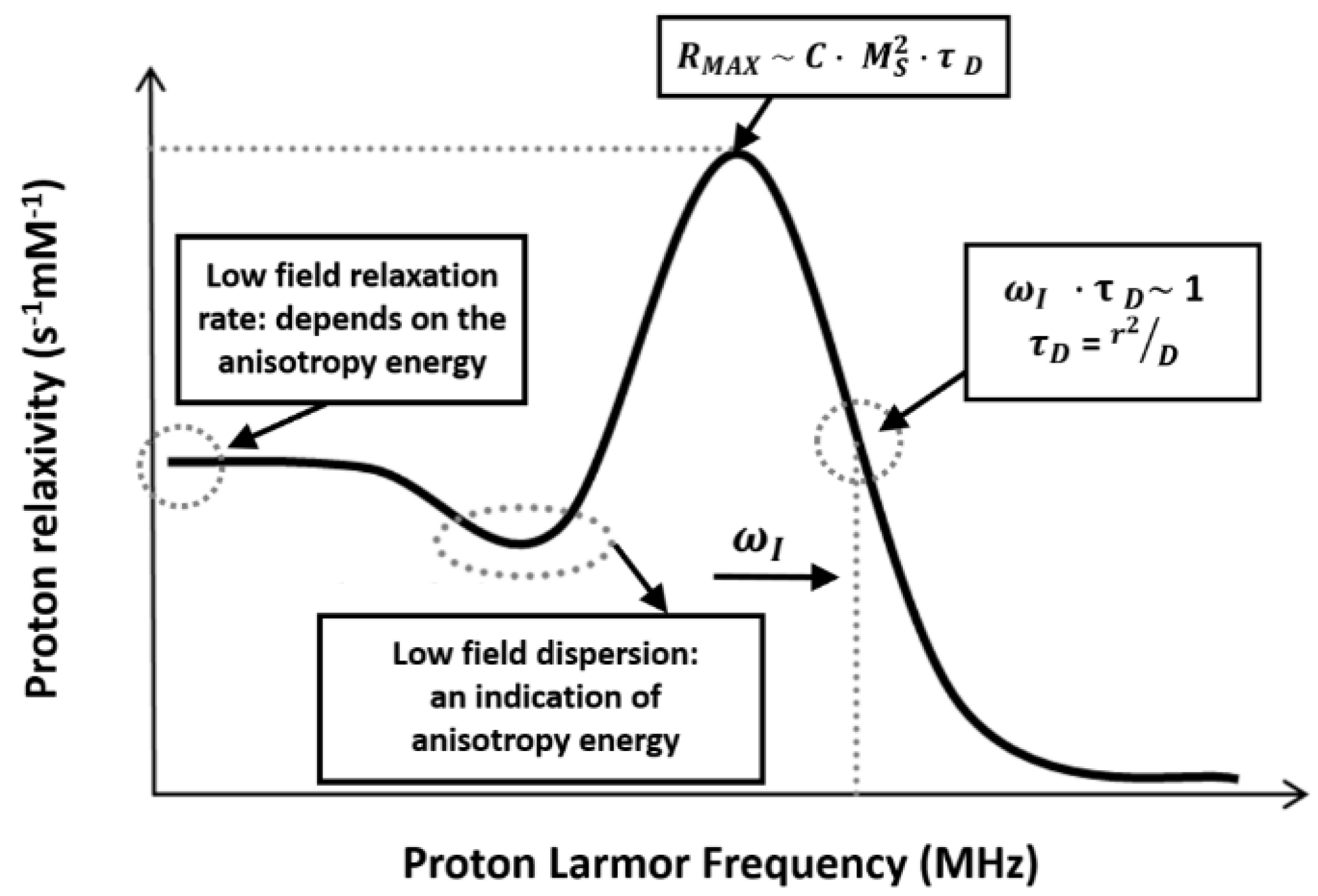
  261. Roch, A.; Muller, R.N.; Gillis, P. Theory of proton relaxation induced by superparamagnetic particles. J. Chem. Phys. 1999, 110, 5403–5411. [Google Scholar] [CrossRef]
  262. Gossuin, Y.; Orlando, T.; Basini, M.; Henrard, D.; Lascialfari, A.; Mattea, C.; Stapf, S.; Vuong, Q.L. NMR relaxation induced by iron oxide particles: Testing theoretical models. Nanotechnology 2016, 27, 155706. [Google Scholar] [CrossRef] [PubMed]
  263. Bordonali, L.; Kalaivani, T.; Sabareesh, K.P.; Innocenti, C.; Fantechi, E.; Sangregorio, C.; Casula, M.F.; Lartigue, L.; Larionova, J.; Guari, Y.; et al. NMR-D study of the local spin dynamics and magnetic anisotropy in different nearly monodispersed ferrite nanoparticles. J. Phys. Cond. Matter 2013, 25, 066008. [Google Scholar] [CrossRef]
  264. Ruggiero, M.R.; Crich, S.G.; Sieni, E.; Sgarbossa, P.; Forzan, M.; Cavallari, E.; Stefania, R.; Dughiero, F.; Aime, S. Magnetic hyperthermia efficiency and 1H-NMR relaxation properties of iron oxide/paclitaxel-loaded PLGA nanoparticles. Nanotechnology 2016, 27, 285104. [Google Scholar] [CrossRef] [Green Version]
  265. Gilchrist, R.K.; Medal, R.; Shorey, W.D.; Hanselman, R.C.; Parrott, J.C.; Taylor, C.B. Selective Inductive Heating of Lymph Nodes. Ann. Surg. 1957, 146, 596–606. [Google Scholar] [CrossRef]
  266. Laurent, S.; Dutz, S.; Hafeli, U.O.; Mahmoudi, M. Magnetic fluid hyperthermia: Focus on superparamagnetic iron oxide nanoparticles. Adv. Colloid. Interface Sci. 2011, 166, 8–23. [Google Scholar] [CrossRef]
  267. Del Bianco, L.; Spizzo, F.; Barucca, G.; Ruggiero, M.R.; Geninatti Crich, S.; Forzan, M.; Sieni, E.; Sgarbossa, P. Mechanism of magnetic heating in Mn-doped magnetite nanoparticles and the role of intertwined structural and magnetic properties. Nanoscale 2019, 11, 10896–10910. [Google Scholar] [CrossRef]
  268. Gas, P.; Miaskowski, A. Specifying the ferrofluid parameters important from the viewpoint of magnetic fluid hyperthermia. In Proceedings of the 2015 Selected Problems of Electrical Engineering and Electronics (WZEE), Kielce, Poland, 17–19 September 2015; pp. 1–6. [Google Scholar] [CrossRef]
  269. Bunaciu, A.A.; Udriştioiu, E.G.; Aboul-Enein, H.Y. X-ray diffraction: Instrumentation and applications. Crit. Rev. Anal. Chem. 2015, 45, 289–299. [Google Scholar] [CrossRef]
  270. Giron, D. Thermal analysis and calorimetric methods in the characterisation of polymorphs and solvates. Therm. Acta 1995, 248, 1–59. [Google Scholar] [CrossRef]
  271. Vyazovkin, S. Thermal analysis. Anal. Chem. 2010, 82, 4936–4949. [Google Scholar] [CrossRef] [PubMed]
  272. Garcia Casillas, P.E.; Rodriguez, C.; Martinez Perez, C. Infrared Spectroscopy of Functionalized Magnetic Nanoparticles. In Infrared Spectroscopy—Materials Science, Engineering and Technology, Theophile Theophanides; IntechOpen: London, UK, 2012. [Google Scholar] [CrossRef] [Green Version]
  273. Skoglund, S.; Hedberg, J.; Yunda, E.; Godymchuk, A.; Blomberg, E.; Odnevall Wallinder, I. Difficulties and flaws in performing accurate determinations of zeta potentials of metal nanoparticles in complex solutions-Four case studies. PLoS ONE 2017, 12, e0181735. [Google Scholar] [CrossRef] [PubMed] [Green Version]
  274. Robson, A.L.; Dastoor, P.C.; Flynn, J.; Palmer, W.; Martin, A.; Smith, D.W.; Woldu, A.; Hua, S. Advantages and Limitations of Current Imaging Techniques for Characterizing Liposome Morphology. Front. Pharmacol. 2018, 9, 80. [Google Scholar] [CrossRef] [PubMed] [Green Version]
  275. Sylvester, P.W. Optimization of the tetrazolium dye (MTT) colorimetric assay for cellular growth and viability. Methods Mol. Biol. 2011, 716, 157–168. [Google Scholar] [PubMed]
  276. Rampersad, S.N. Multiple applications of Alamar Blue as an indicator of metabolic function and cellular health in cell viability bioassays. Sensors 2012, 12, 12347–12360. [Google Scholar] [CrossRef] [PubMed]
  277. Riss, T.L.; Moravec, R.A.; Niles, A.L.; Duellman, S.; Benink, H.A.; Worzella, T.J.; Minor, L. Cell Viability Assays. In Assay Guidance Manual [Internet]; Sittampalam, G.S., Grossman, A., Brimacombe, K., Eds.; Eli Lilly & Company and the National Center for Advancing Translational Sciences: Bethesda, MD, USA, 2004. Available online: https://0-www-ncbi-nlm-nih-gov.brum.beds.ac.uk/books/NBK144065/ (accessed on 1 June 2019).
  278. Patil, U.S.; Adireddy, S.; Jaiswal, A.; Mandava, S.; Lee, B.R.; Chrisey, D.B. In Vitro/In Vivo Toxicity Evaluation and Quantification of Iron Oxide Nanoparticles. Int. J. Mol. Sci. 2015, 16, 24417–24450. [Google Scholar] [CrossRef] [PubMed]
  279. Oancea, M.; Mazumder, S.; Crosby, M.E.; Almasan, A. Apoptosis assays. Methods Mol. Med. 2006, 129, 279–290. [Google Scholar]
  280. Macías-Martínez, B.I.; Cortés-Hernández, D.A.; Zugasti-Cruz, A.; Cruz-Ortíz, B.R.; Múzquiz-Ramos, E.M. Heating ability and hemolysis test of magnetite nanoparticles obtained by a simple co-precipitation method. J. Appl. Res. Technol. 2016, 14, 239–244. [Google Scholar] [CrossRef] [Green Version]
  281. Chen, D.; Tang, Q.; Li, X.; Zhou, X.; Zang, J.; Xue, W.Q.; Xiang, J.Y.; Guo, C.Q. Biocompatibility of magnetic Fe3O4 nanoparticles and their cytotoxic effect on MCF-7 cells. Int. J. Nanomed. 2012, 7, 4973–4982. [Google Scholar] [CrossRef] [Green Version]
Figure 1. Ferromagnetic material hysteresis curves expressed as M vs. H (a) and B vs. H (b) curves. Legend: Ms is the saturation magnetization, Mr is the remnant magnetization at H = 0, Hci is the intrinsic coercivity, Br is the remnant induction (or remanence) at H = 0, and Hc is the coercivity. For hard magnets: HciHc; for soft-magnets: HciHc. Reprinted with permission from [40], published by Elsevier, 2003.
Inorganics 08 00006 g001
Figure 2. Magnetization (hysteresis) curves associated with the different classes of magnetic materials (i.e., Hard/Soft-ferromagnetics, superparamagnetics, diamagnetics, and paramagnetics).
Inorganics 08 00006 g002
Figure 3. Schematic representation of ferromagnetic domains in absence (left) and in presence (right) of an external magnetic field applied. In the latter case, boundaries are dashed since when domains are aligned (right panel), the sample reaches the saturation point and there are not any domains walls.
Inorganics 08 00006 g003
Figure 4. Hysteresis loops obtained at T = 2 K for sample oriented at 0°, 45°, and 90° in respect of the direction of external magnetic field. Reprinted with permission from [46], published by John Wiley & Sons, 2017.
Inorganics 08 00006 g004
Figure 5. Effect by temperature variations on the phase crystal structure and magnetic structure organization. Panel (a) spinel-type oxide MnV2O4 crystal structure A-site are surrounded by oxygen tetrahedron and B-site ions by octahedron. The V3+ ion has orbital degeneracy in the t2g orbital. Panel (b) The collinear ferrimagnetic structure. Panel (c) Magnetic structure in the non-coplanar ferrimagnetic tetragonal phase (c < a). Reprinted with permission from [48], published by Elsevier, 2018.
Inorganics 08 00006 g005
Figure 6. Magnetization curves of FePt nanomaterials. Panel (a) ferromagnetic Fe3Pt nanocrystals. Panel (b) predominantly paramagnetic FePt3 nanocrystals. Reprinted from [55] (published by MDPI, 2018) licensed under CC BY 4.0.
Inorganics 08 00006 g006
Figure 7. Summary of the main relevant forms of magnetism and their features. Reprinted with permission from [57], published by Woodhead Publishing and Elsevier, 2016.
Inorganics 08 00006 g007
Figure 8. Electromagnetic spectrum from infrared (IR) to γ-rays and some probes for the magnetic imaging.
Inorganics 08 00006 g008
Figure 9. (a) Patterns obtained from Fe2O3 nanoparticles on an iron-silicon alloy (Bitter technique) in large fields (16× magnification). The observed striations were found perpendicular to the applied magnetic field without any relationship to the grain structure for large magnetizations. Reproduced with permission from [132], published by American Physical Society, 1931; (b) representation of the magnetic domain viewer (modified Bitter technique). The technique employs a coil to generate a magnetic field perpendicular to the surface of the sample. Magnetization directions are shown into (X) and out of (O) the plane, respectively; (ce) representations of the longitudinal, polar magneto-optical Kerr and magneto-optical Faraday effect configurations, respectively; (f) magneto-optical imaging of a thin ferromagnetic film using a diamond-based sensor. Reprinted from [122] (published by Nature Publishing Group, 2016) licensed under CC BY 4.0; (g) optical (left panel) and Kerr images (right panels) of a few-layered Cr2Ge2Te6 crystal exfoliated on SiO2/Si obtained at different T. The layer number (2L, 3L, or 4L) is indicated by arrows in (g). Scale bars in (g) are 10 μm. Image adapted from [133], published by Springer Nature, 2017.
Inorganics 08 00006 g009
Figure 10. (ac) representations of type-I, type-II, and type-III magnetism in SEM, corresponding to SE, BSE, and polarized electron detections, respectively; (d) Nd, Fe elemental distributions (left panels), topography and magnetic domain images (right panels) of a NdFeB permanent magnet. Element maps were acquired by Auger spectroscopy. Panels in (d) are adapted from [116], published by Oxford Academic, 2013.
Inorganics 08 00006 g010
Figure 11. Lorentz microscope (a) in-focus; (b) overfocus and underfocus Fresnel mode TEM imaging; (c) Foucault mode; (d) the related magnetic contrast imaging; (e) domain wall contrast inversion in Fresnel mode; (f) scheme of the inverse bright/dark contrast corresponding at the positions of the magnetic domain walls in defocused Fresnel; and (g) bright-field Fresnel-mode L-TEM image sequence (1–5) of an isolated DW skyrmion collected with a different tilting angle and the corresponding in-plane magnetic induction maps (6–10) as obtained by TIE. Panel g reprinted with permission from [152], copyright by American Physical Society, 2019.
Inorganics 08 00006 g011
Figure 12. (a) scheme of the differential phase contrast (DPC) technique in L-STEM; (b,c) L-STEM images of a Fe nanostructure (from Fe exacarbonyl by EBID) with its in-plane components; (d) DPC color image (representation of the color wheel shown in the top-right inset) and (e) the profile of the line selected in (c) showing the induction profile, as measured from the deflection angle at the vortex core. βL is Lorentz deflection angle. Panels b–e are reprinted with permission from [153], copyright by Elsevier, 2015.
Inorganics 08 00006 g012
Figure 13. (a) Schematic diagram showing interference fringe formation from the overlap of the sample and reference waves by the electron biprism, adapted from [155], published by Wiley, 2010. Electron holography (EH) images of a Co nanowire 9 nm thick and 30 nm long: (b) electrostatic and (c) magnetic contributions to the electron beam phase shift; the magnetic flux deduced from the magnetic phase image is superimposed over the electrostatic phase shift image; (d) the cosine of 38 times the magnetic phase image that allows a better visualization of the magnetic flux within and out of the nanowire; (e) phase shift profile extracted from the right part of panel (d) where the magnetic induction is constant; (be) reproduced with permission [156], copyright (2011) by American Chemical Society. (f) Electron hologram of a Fe3O4 nanoparticle exposing well-resolved interference fringes; (g) representation of the tilting operation to obtain the in-plane magnetization component to the total phase shift; (h) magnetic contribution to the total phase shift; (i) Cosine of the magnetic contribution to the phase shown in (g) to produce contours with a spacing of 0.53 radians; (j) direction of the projected in-plane magnetic induction in the Fe3O4 nanoparticle as obtained with the addition of colors; and (k) the final magnetic induction map that shows the strength and direction of the magnetic signal in the Fe3O4 nanoparticle and the stray magnetic field. (fk): panels are adapted from [157], published by Wiley, 2019.
Inorganics 08 00006 g013
Figure 14. (a) Principles and (b) forces acting between the tip and the magnetic surface in MFM; (c) phase and (d) amplitude shifts associated with the long-range magnetic interactions; (e) topography signal (top panel) and height profiles (bottom panel) of pyrolyzed magnetic chitosan nanoparticles imaged on the freshly cleaved mica support; (f) magnetic force microscopy (MFM) phase shift images obtained at various lift heights (H = 90, 100, 110, and 120 nm); (g) forward and backward amplitude and phase maps obtained for H = 90 nm above the sample surface (obtained at constant height of 90 nm). Reproduced with permission from [65], copyright (2016) by American Chemical Society; (hj) MFM maps acquired at T = 18.28 K, T = 18.23 K, and T = 9.95 K without a magnetic field. In the bottom insets, profiles of the phase signal along selected lines of the three structures are illustrated. Panels (hj) are adapted from [165], published by American Association for the Advancement of Science, 2018.
Inorganics 08 00006 g014
Figure 15. (a,b) representation of the spin polarized scanning tunneling microscopy (SP-STM) principle. In magnetic materials the density of states largely depends on the two different spin orientations: Parallel (higher tunneling current) or antiparallel (lower tunneling current) one; (c,d) spin-polarized tunneling conductance maps for Co phatolocyanine taken at −0.32 V and −0.16 V (image size: 40 × 20 nm2); (e) map of a selected region in (c) (2.6 × 2.6 nm) with molecular structure model superimposed. Reprinted with permission from [170], copyright 2008 by American Physical Society; (f,g) topographies (top panels) and the associated spin-resolved differential conductance maps (bottom panels) of a single TbPc2 molecule laying on a metal Co-layered Ir (111) surface for parallel (left panels) and antiparallel (right panels) magnetization alignments. In the top insets of (f) and (g) schemes of the operational conditions with the superimposed molecular structure model of TbPb2, are illustrated. Adapted from [171], published by Nature Publishing Group, 2012.
Inorganics 08 00006 g015
Figure 16. (af) elemental maps of the NPs: (a) Fe, (b) Co, and (c) Ni nanoparticles; (df) the corresponding magnetic contrast images. Dashed and solid circles represent NPs in the superparamagnetic and magnetically blocked states, respectively. Au markers shown in the images are used for the particle identification. Reproduced with permission from [178], copyright (2017) by American Physical Society. (gk) multitechnique imaging of a Fe3O4 (magnetite) island on an FeO wetted layer on the Ru(0001) surface: (g) LEEM image (electron energy = 8 eV), (h) XAS image of the same area acquired at a photon energy close to the maximum of the L3 Fe absorption edge, (i) X-ray magnetic circular dichroism image of the same area, (j) low-energy ED pattern acquired from the island at 30 eV. One of the ED spot, characteristic of the spinel phase is shown by a circle. (k) XAS spectrum of the island showing the L3 and the L2 Fe edges and XMCD spectrum taken in the black domain in (i). Reproduced with permission from [179], published by The Royal Society of Chemistry, 2018.
Inorganics 08 00006 g016
Figure 17. (a) representative scheme of the Talbot Lau neutron tomography setup; (b) representation of the investigated wedge-shaped FeSi single crystal, radiographic projection images as obtained by Talbot-Lau neutron dark-field radiography; (ci) the same radiographic projection images obtained under an external magnetic field (parallel to the cylinder axis) of 11 mT, 20 mT, 40 mT, 84 mT, 225 mT, and 11 mT. The dark stripes are caused by domain walls that are nearly parallel to the incident beam. Adapted from [186], published by Nature Publishing Group, 2010.
Inorganics 08 00006 g017
Figure 18. (a) Representation of the wide-field magnetic imaging microscope field fluorescence microscope setup vector plots of the measured (red arrows, left panel) and simulated (blue arrows, right panel) magnetic field projections in the xy plane are reported superimposed; (b,d) optical and (c,e) backscattered electron (BSE) images, respectively. Adapted from: [123], published by Nature Publishing Group, 2013.
Inorganics 08 00006 g018
Figure 19. (Left) Physicochemical factors that affect cellular uptake of nanoparticles: Surface charge, size and shape. (Right) Different morphologies of iron oxide nanoparticles. Reproduced with permission from: [206], published by Ivyspring, 2018.
Inorganics 08 00006 g019
Figure 20. Left: schematic representation of the experimental setup for dynamic light scattering measurements. Right: TEM micrographs of Fe3O4 magnetic nanoparticles with the corresponding size distribution determined by DLS. The Z-average of magnetic nanoparticles measured by DLS is 16.9 ± 5.2 nm (top), 21.1 ± 5.5 nm (middle), and 43.1 ± 14.9 nm (bottom), respectively. Reproduced with permission from [228] (published by Springer Open, 2013) licensed under CC BY 2.0.
Inorganics 08 00006 g020
Figure 21. Schematic representation of the two layers forming the electric double layer (EDL) developed on a negatively charged particle. The inner layer, called the Stern layer, is composed by ions of charge opposed to the particle surface, i.e., positive ions in this case. The outer layer, also known as diffuse layer, is made up of both negative and positive charges. The Zeta Potential is the electrokinetic potential at the slipping plane.
Inorganics 08 00006 g021
Figure 22. Left: Schematic of soft and hard corona formed on the surface of a NP. Reproduced with permission from Bhattacharjee et al. [229], copyright by Elsevier 2016. Right: schematic representation of loss of transferrin receptor targeting for transferrin-conjugated nanoparticles in the presence of corona proteins. Adapted from Salvati et al. [250], published by Springer Nature, 2013.
Inorganics 08 00006 g022
Figure 23. Biomedical applications of magnetic nanoparticles.
Inorganics 08 00006 g023
Figure 24. Nuclear magnetic relaxation dispersion (NMRD) profile of magnetite particles in colloidal solution.
Inorganics 08 00006 g024
Table 1. Magnetic imaging methods and their characteristics.
Method(s)QuantitativeResolution (nm)Complexity *Acquisition TimeVacuum Req.Sample Thickness (nm)Info on Depth (nm)External Magn. FieldSelected Depth InfoHigh, Low Temperature ***Types of Specimen ****Ref.
BestTipical
BitterN~100500L<s-No limit500YesLNoS, TF, NPs[109]
Magneto-opticY300>500L<s-No limit20YesLCryo/VTS, TF, NPs[24,110,111]
L-TEMY2050M<sHV<100–150ST **YesNoVTS, TF, NPs[24,112,113]
DPCY320H<sHV VTS, TF, NPs[24,114]
Electron holographyY520H1–10 sHV<150ST **YesNoVTS, TF, NPs[113,115]
SP-SEMY10100H1–100 minUHVNo limit1–2LowHVTS, TF, NPs[24,116]
XMCDY300500H1–10 minUHVNo limit<5–10-HVTS, TF, NPs[95,117,118]
TXMCDY3060H1–10 s-<150ST **YesHVTS, TF, NPs[95]
SPLEEMY340H1 s–10 minUHVNo limit1–2-VHVTS, TF, NPs[95]
MFMN20–30100L/M5–30 minAir, HV No limit20–500YesNoCryo/VT.S, TF, NPs[24,119,120]
SP-STMN/Y≤12–3M10–100 min(air), HVNo limit<1–2YesVHCryo/VT.S, TF, NPs of metals/semic.[24,121]
N-V DiamondY400 L<sNo NoYesNoNoS, TF, LM[122,123]
TXMsY10–1550M/Y<10 s-No limitST **YesHVTS, TF, NPs, B[117,121,124,125,126,127]
Neutron techniques Tens of µm VHsNo5–1002–3YesNoVTLM; S, TF (pol. neutron reflectom.), NPs (SANS)[117,128,129,130]
* L = low, M = medium, H = high, VH = very high; ** ST = sample thickness; *** Cryo = cryogenic temperature, VT = variable temperature; **** S = surfaces, TF = thin films, LM = living matter, NPs = nanoparticles, B = bulk.
Table 2. Main properties of the techniques reported in the previous paragraph, useful to characterize magnetic systems designed for biomedical applications.
Method(s)Information ProvidedAcq. TimeComplexitySample FormAdvantagesDrawbacksRef.
X-ray DiffractionCrystalline structure; crystal size, strain, defects; particle size; sample purity; iron oxide proportion<20 minLSolid, liquid Qualitative and quantitative analysis; powerful and rapid; minimal sample preparation requiredSize limit (better results are obtained with large crystals); high amount of material needed (g); possible misleading results interpretation (peaks overlay)[269]
Thermal Analysis (DTA, pc-DSC, TGA, µ-TGA)Thermal stability; water adsorption; molecule adsorption; phase transition temperature; crystallinity and puritymin–hoursM-HSolid, liquidQualitative and quantitative analysis; low amount of sample needed (mg–g)Challenging results interpretation; challenging results comparison between laboratories; strong dependence of DTA signals from experimental conditions[270,271]
Mössbauer SpectroscopySize of magnetic core; magnetic interactions; precise identification of iron oxides; magnetite and maghemite discrimination; blocking temperaturemin–hoursHSolidLow amount of sample required (1–5 mg); valence state of iron in minerals detectable; best technique to identify different iron oxidesLow spatial resolution; thinly spread powders needed; the optimal amount of sample should be selected each time; data analysis techniques complex and variable; low number of elements suitable to be investigated; very low temperatures required[104,223]
IR Spectroscopy; FTIR spectroscopyMaterial structure; chemical Bonds; surface coating/functionalization of magnetic NPsminLSolid, liquidSimplicity and availability; non expensive technique; qualitative and quantitative analysis; fast mean of identification in case of magnetite; high sensitivity (µg)Complex mixtures are hardly analyzed; functional groups cannot be exactly located[272]
Dynamic light scattering (DLS)Hydrodynamic radius of NPs; polydispersity of the sample; aggregation of NPs; adsorption of protein corona<5 minLLiquidWide sampling of the specimen; speed and ease of measurement; estimation of the radius of solvated particles; accessible and automated process; high sensitivity to small aggregates; small amount of sample required (µL)Highly polydispersed, diluted or fluorescent samples cannot be measured accurately[227,228,229,231]
Zeta PotentialApparent surface potential of NPs; adsorption of protein corona<5 minLLiquidWide sampling of the specimen; speed and ease of measurement; accessible and automated process; small amount of sample required (µL)Highly polydispersed samples cannot be measured accurately; measurements influenced by pH, ionic strength, dispersion media; measurements affected by sample sonication; measurements affected by fast metal/ion release [273]
SEM
TEM
Size of the magnetic core; morphology; size distribution; homogeneity; surface structureminL/MSolidAccurate information provided on size of magnetic core; images of NPs are displayed; very high magnification possibleLong and complex sample preparation; expensive technique; cryo-EM is needed for samples sensitive to temperature; low sampling of the specimen; absence of information about sample aggregation in liquid suspensions; highly qualified personnel needed; possible artifacts formation; vacuum needed[274]
NMRD Profile FittingNanomagnet crystals (N.C.) average radius; N.C. Néel relaxation time; N.C. anisotropy energy; N.C. specific magnetization; possible NPs clustering; longitudinal Relaxivity R1 at different magnetic fields; MRI efficiency predictionhoursHLiquidMultiplicity of information provided in one fitting; prediction of MRI efficiencyHighly specific instrumentation required; samples must be in liquid form and stable during the acquisition time; staff must be highly trained[261,262]
Note: L = low, M = moderate, H = high.
Table 3. Comparison between some of the most diffuse toxicity assays, useful to evaluate potential toxic effects exerted by magnetic NPS.
AssayParameter MeasuredInformation ProvidedMeasurem. MethodAdvantagesDrawbacksRef.
MTTMitochondrial activityPossible cytotoxic effects of compounds/drugs/NPsFluorescence AbsorbanceInexpensive; high throughput screening; low amount of sample neededOperator and procedure dependent (e.g., cell density, culture medium and MTT exposure time); Substrate conversion needed[277]
Alamar Blue (Resazurin)Cellular metabolic activityPossible cytotoxic effects of compounds/drugs/NPsFluorescence AbsorbanceInexpensive, High throughput screening; low amount of sample needed; more accurate than MTTOperator and procedure dependent (e.g., cell density, culture medium and MTT exposure time); substrate conversion needed[277]
Trypan Blue Exclusion TestMembrane integrityPossible cytotoxic effects of compounds/drugs/NPs Number of dead/viable cellsOptical microscopyInexpensive; extremely rapid assay; no substrate conversion neededOperator dependent; possible interference in case of incubation with colored/fluorescent samples[277]
ATP detectionATP synthesisPossible cytotoxic effects of compounds/drugs/NPs; number of viable cellsLuminescenceFast assay; high sensitivity; less artifacts occurrence; no substrate conversion neededExpensive[277]
ROS productionGeneration of ROS *Possible cytotoxic effects of compounds/drugs/NPs; cell oxidative stressFluorescenceInexpensiveSubstrate conversion needed[278]
Hemolysis AssayRed blood cell lysisHemolytic power of compounds/drugs/NPsUV–vis spectroscopyExtremely useful in view of (pre)clinical applications; possibility to run the test in plasmaRed blood cells of the chosen specie needed[280]
* ROS: Reactive Oxygen Species.

