Measuring the Spatial Noise of a Low-Cost Eye Tracker to Enhance Fixation Detection


1
Department of Geography, Ghent University, 9000 Gent, Belgium
2
Polytech Nantes, Laboratoire des Sciences du Numérique de Nantes (LS2N), Université de Nantes, 44306 Nantes CEDEX 3, France
3
Department of Surveying & Geoinformatics Engineering, University of West Attica, 12243 Aigaleo, Greece
*
Author to whom correspondence should be addressed.
J. Imaging 2018, 4(8), 96; https://0-doi-org.brum.beds.ac.uk/10.3390/jimaging4080096
Submission received: 1 June 2018
/
Revised: 5 July 2018
/
Accepted: 25 July 2018
/
Published: 28 July 2018
Abstract
:The present study evaluates the quality of gaze data produced by a low-cost eye tracker (The Eye Tribe©, The Eye Tribe, Copenhagen, Denmark) in order to verify its suitability for the performance of scientific research. An integrated methodological framework, based on artificial eye measurements and human eye tracking data, is proposed towards the implementation of the experimental process. The obtained results are used to remove the modeled noise through manual filtering and when detecting samples (fixations). The outcomes aim to serve as a robust reference for the verification of the validity of low-cost solutions, as well as a guide for the selection of appropriate fixation parameters towards the analysis of experimental data based on the used low-cost device. The results show higher deviation values for the real test persons in comparison to the artificial eyes, but these are still acceptable to be used in a scientific setting.
1. Introduction
Eye movement analysis constitutes one of the most popular ways to examine visual perception and cognition. The effectiveness of the method can be easily proved by the wide range of applications in several research disciplines, including: Research in psychology [1], human-computer interaction (HCI) and usability [2,3], training [4] and learning processes [5], marketing [6], reading behavior [7], etc. Eye tracking techniques allow capturing the visual reaction in an objective way. Considering the complexity of the spatiotemporal distribution of eye tracking data, the need for robust analysis techniques to efficiently process the recorded signals is well-known from the early eye movement surveys [8,9]. The analysis of eye tracking protocols is connected with the implementation of fixation identification algorithms, which constitute the basis for the development of other analysis software tools. Over the last years, different fixation identification algorithms have been proposed by the eye tracking community (e.g., [10,11,12,13]), while at the same time several eye movement analysis tools have been developed. It is worth mentioning that the last decades several toolboxes, libraries, and/or standalone, such as ILAB [14], OGAMA [15], GazeAlyze [16], EyeMMV [12], ETRAN [17], and ASTEF [18,19], have been proposed and distributed as open-source projects.
The wide acceptance of eye tracking methods in both basic and applied research disciplines resulted in a technological revolution of the recording devices. Modern approaches of eye localization are based on ordinary webcams (e.g., References [20,21,22]), which also holds true for low-cost eye trackers (e.g., References [23,24,25]). These types of eye tracking devices have several advantages in comparison with the traditional ones, as they have a low-cost and a typically a small size, which facilitates their transport and the use of multiple trackers at the same time [26]. An excellent presentation of the current panorama in low-cost eye tracking services (methods, datasets, software etc.) is provided in a recent review article by Ferhat and Vilariño (2016) [27].
Among the existing commercial devices, Eye Tribe (The Eye Tribe©, The Eye Tribe, Copenhagen, Denmark) has already been used in several research studies and applications (e.g., References [28,29,30,31]). Based on the results of a recent study, presented by [26], the accuracy and the precision of this device may be considered comparable with these of well-established trackers. Despite the fact that this type of low-cost eye trackers can be served as excellent utilities for HCI applications (e.g., typing using only the eyes and virtual keyboards, manipulate software applications etc.), a large challenge is to verify if these devices can be used for scientific purposes. For this it is essential to verify the captured signal’s quality (i.e., accuracy and precision), under real experimental conditions, while at the same time selecting the appropriate experimental set-up (i.e., sampling frequency, recording software, distance between monitor and participant, analysis parameters) [26,32].
In the present study, two researchers combined their previous experience the field of eye movement research: (1) The evaluation of the Eye Tribe Tracker’s accuracy, which also includes a statistical comparison with other eye trackers (e.g., SMI RED [26]), and (2) the development of a fixation detection algorithm, capable of removing spatial noise (EyeMMV [12]). The proposed work is a combined follow-up study on these two independent initiatives.
An integrated methodological framework, based on artificial eyes measurements and human eye tracking data, is proposed for the implementation of the process. The results of this work aim to serve as a reference for the verification of the validity of low-cost solutions in scientific research and the enhancement of the resulting fixation detections through the selection of appropriate parameters for noise removal (e.g., using EyeMMV’s algorithm).
2. Related Work
2.1. The Eye Tribe and its Low-Cost Eye Tracker
When it was founded in 2011, the ambition of the company “The Eye Tribe” was “to make eye tracking available for everyone at an affordable price”. In 2014, they started shipping their first eye tracker with the slogan that it was “The world’s first $99 eye tracker with full SDK” [26]. The specifications of this device can be found in Table 1. It is a very small and lightweight eye tracker, making it flexible to transport and use. Furthermore, it can be placed ‘freely’—for example, beneath a laptop screen, underneath a monitor on a small tripod (standardly included in the package), or optionally attached to a tablet.
Although this eye tracking system was not accompanied by a fully-fledged software package to set-up and conduct analyses, it got picked up by researchers rather quickly. A search of Google Scholar resulted in a list of more than 50 research publications which at least mention the Eye Tribe eye tracker. From this list, six were already published in 2014 already, and 25 in 2015. Because of this recent evolution it is not surprising that the majority of these publications were conference contributions, a much smaller portion of journal articles were counted. The remainder of the publications were master theses or other reports. Furthermore, the research fields of these publications are also diverse, including: Human-computer interaction, psychology (including sub-fields such as perception, cognition, and attention), computer science, eye tracking, medicine, gaze as input, and education.
As was indicated before, The Eye Tribe eye tracker was not used in all publications, others just mention its existence. From this large collection of publications, three deserve special attention because they focus on evaluating the eye tracking device itself. Dalmaijer (2014) [32] was the first to question whether this new low-cost eye tracker could be used for research purposes. He compared the accuracy and precision of the tracker from The Eye Tribe (60 Hz sampling rate) with that of the high-quality Eye-Link100 (from SR Research, 1000 Hz sampling rate). He concluded that the device was suitable for analyses related to fixations, points of regard and pupillometry, but that the low sampling rate hinders it use for high-accurate saccade metrics. The paper also introduces some open-source toolboxes and plugins (e.g., Pytribe, PyGaze plugin for OpenSesame, and Eye Tribe Toolbox for Matlab) to communicate with the Eye Tribe Tracker. This study was further extended by Ooms et al. (2015) [26], who measured the accuracy and precision of the Eye Tribe Tracker at 30 Hz and 60 Hz, comparing the recordings registered through different tools (JAVA using the API and OGAMA) and applying different fixation detection tools (OGAMA and EyeMMV). The obtained results were compared with those registered with a high-qualitative eye tracker from SMI (RED250) which recorded eye movements at 60 Hz and 120 Hz. These authors also concluded that, when set-up correctly and used in a correct context, the Eye Tribe tracker can be a valuable alternative for the well-established commercial eye trackers. Popelka et al. (2016) [33] also compared the results of the Eye Tribe tracker with those registered with an SMI RED250, but they performed a concurrent registration with both eye trackers. The data recorded from the Eye Tribe tracker was registered using HypOgama, which is a combination of OGAMA (to record the eye tracking data itself) and Hypothesis (to register additional quantitative data). They also registered minimal deviations between both systems.
When focusing on the studies which actually used the eye tracker, most of them did not mention the sampling rate at which the recordings were registered. Nevertheless, the experiments had to be set-up, the data registered and finally analyzed using some kind of software. Most of them do not mention specific software or indicate they used the accompanying SDK (e.g., PeyeTribe—a python interface) [34]. Other authors managed to combine the Eye Tribe tracker with other equipment such as EEG or Emotive EPOC [29,35].
2.2. Research with Webcams or DIY Eye Trackers
Besides the rise of the commercially available low-cost eye trackers, such as the Eye Tribe Tracker, other related trends could be noticed in scientific research: Do-it-yourself (DIY) or home-made eye trackers. These DIY eye trackers are typically constructed using a webcam and an IR light source (e.g., Reference [23]). These eye trackers are also often accompanied by custom made open-source software tools, such as open Eyes [36], ExpertEyes [25] and ITU Gaze-Tracker [37]. The reported costs for these DIY eye trackers varies from 17 to 70 euros and the reported accuracies from “less than 0.4°” [25] to 1.42° [23].
Recently, webcams (stand-alone or integrated in a laptop, without additional IR-lighting) are also used to track a users’ eyes (e.g., Reference [38]). This new trend would be a great revolution in eye tracking research, making it possible to conduct eye tracking research at a distance with nearly any user that works with a device that contains a camera or webcam. Because no additional IR light source is used, eye trackers solely based on a webcam take a different approach. Gómez-Poveda and Gaudioso (2016) [21] describe a multi-layered framework, based on (1) face detection; (2) eye detection, and (3) pupil detection. They evaluated this approach using three different cameras. WebGazer is such an eye tracking system that is available online which can connect to any common webcam [21]. To use the webcam as an eye tracker, the user has to calibrate the system by watching certain points on the screen in a game-like setting. Similar examples of such online services are EyeTrackShop (http://eyetrackshop.com) and GazeHawk [39]. Interesting to note is that the latter joined Facebook. Other companies that offer webcam-based eye tracking are Xlabs (http://xlabsgaze.com/) and EyeSee (http://eyesee-research.com/). Another example is TurkerGaze, which is linked with Amazon Mechanical Turk (AMTurk) in order to support large-scale crowdsourced eye tracking [20].
2.3. Eye Tracking Data Quality
Eye tracking data quality is related to the raw data produced by eye tracking devices [40]. Data quality can be mainly expressed by two measures; accuracy and precision. Accuracy refers to the difference between the measurement and the real eye position, while precision characterizes the consistency among the captured data [21]. These measures are also discussed in detail and applied in the paper of the study that precedes the current experiments [26]. According to Holmqvist et al. (2012) [41], the overall quality of eye tracking data is a subject of several factors, including participants, operators, executed tasks, recording environment, geometry of the system camera-participant-stimulus, and the eye tracking device. Additionally, more specific factors, such as calibration process, contact lenses, vision glasses, color of the eyes, eyelashes and mascara [42], as well as participants’ ethnicity and experimental design [43], may also have a critical role. Furthermore, it is worth mentioning that recent studies also examine the affection of additional parameters (e.g., head and position movements) in the case of infants (e.g., Reference [44]). As it becomes obvious, issues related to data quality are considered very important for the performance of eye tracking experimentation in both stable and removable devices (see e.g., the work described by Clemotte, et al. (2014) [45] about a remote eye tracker model by Tobii), DIY devices (see e.g., the recent work of Mantiuk (2016) [46]) and low-cost devices (see e.g., the recent evaluation of Tobii Eye X Controller described by Gibaldi, et al. (2016) [47]). Except from the aforementioned research studies, an extended description and discussion about the eye tracking data quality measures can be also found in a research article by Reingold (2014) [48].
The computation of the accuracy of an eye tracking device can be based on the collection of real (human) eye tracking data, during the observation of fixed targets, with uniform (or not) spatial distribution, projected on a computer monitor or observed within a real or 3D virtual environment (for the case of mobile devices). This procedure is also able to validate the process of eye tracker calibration and to serve as an indicator of the recording uncertainty. For example, in a research study presented by Krassanakis, et al. (2016) [49], the calibration process is validated based on the performance of the fuzzy C-means (FCM) algorithm clustering, using as number of clustering classes and the number of fixed targets. Generally, the use of fixed targets and the calculation of the performed accuracy, before and after the presentation of the experimental visual stimuli, may serve as a quantitative indicator of calibration quality and the quality of the collected gaze data [12,50,51,52,53].
The complexity of eye tracking data can already be derived from the fact that the sampling rates of the available eye tracking devices can vary between 25–2000 Hz [40]. Therefore, the aggregation of eye tracking events in fundamental metrics (i.e., fixations and saccades) is a crucial process. Moreover, the results of this process are directly connected with the quality of the recorded data, as well as with the implemented algorithms for events detection (see also the section Fixation identification algorithms and thresholds).
Since accuracy depends on real gaze data, the eye trackers’ precision can be measured through the use of artificial eyes (e.g., References [49,54,55] and the computation of root mean square (RMS) error, sample distances, or standard deviation metrics [56]. For example, Wang et al. (2016) [55] present an extensive examination on different types of artificial eyes in conjunction with different eye tracking devices. More specifically, Wang et al. (2016), using four models of artificial eyes, examined monocular and binocular devices—with sampling rates and precisions (as reported by the manufacturers) in the ranges 30–1000 Hz, and 0.01°–0.34°, correspondingly, while a comparison with real gaze data is also implemented. The results of studies, such as those presented by Wang et al. (2016) [55], may serve as critical guides to set-up experimental designs and the analysis of the resulting data. Since, artificial eyes seem an effective way to evaluate the precision of eye tracking devices, it is worth mentioning that other approaches simulate the eyes using render images produced by 3D models (e.g., Reference [57]).
2.4. Fixation Identification Algorithms and Thresholds
Although the accuracy of eye trackers is determined solely on raw data, it is important to consider the algorithms that identify the relevant samples. When the noise of a certain eye tracker is (partially) modelled, it can be filtered out when processing the raw data. For a majority of the studies, this fixation detection step has to be carried out anyhow. Fixations and saccades constitute the fundamental events occurred during the performance of any visual procedure. The implementation of event detection algorithms has a direct influence in the next steps of the analysis and in the overall experimental results interpretation.
A basic classification of fixation detection algorithms is proposed by Salvucci and Goldberg (2000) [58]. This taxonomy has been adapted by several research studies (see e.g., the current review article presented by Punde and Manza (2016) [59]). The proposed classification is based on the parameters that can be used for the characterization of fixation events. More specifically, these parameters are related to velocity-based, dispersion-based, or area-based criteria. Among the proposed approaches, dispersion-based (I-DT) and velocity-based (I-VT) algorithms seem to have wide acceptance [60]. Indeed, both commercial (e.g., Tobii, SMI, etc.) and open-source tools (e.g., OGAMA, EyeMMV etc.) are based on I-DT and I-VT types of algorithms. Additionally, there are also research studies, which propose the identification of fixations and saccades by combining criteria inspired by I-DT and I-VT types (see, for example, the research study presented by Karagiorgou, Krassanakis, Nakos, and Vescoukis (2014) [61], and the proposed work by Li, et al. (2016) [62], where the process of events identification is based on the implementation of DBSCAN algorithm).
Except from the selection of the suitable identification algorithm, the used algorithms’ parameters play also a critical role. Different parameter values may produce different outcomes [63]. Therefore, considering the spatiotemporal nature of fixation events, the corresponded spatial and temporal thresholds must be very carefully chosen and adapted to the nature of the executed visual task. As a consequence, several methods have proposed towards the examination on the optimum fixation parameters’ thresholds (see e.g., the analytical/statistical method recently proposed by Tangnimitchok, et al. (2016) [64]). The range of the radius value for the detection of fixation point cluster is well reported in several research studies; reported ranges refer the values between 0.25°–1° [18,58,65] and 0.7°–1.3° [66,67] of visual angle. Similarly, temporal thresholds are also mentioned in the literature and correspond to the minimum duration that may characterize a fixation event. Typical literature refers the values of 100–200 ms [3,65], 100–150 ms [68], 150 ms [69], while in other studies report also the value of 80 ms as the minimum value [70].
3. Materials and Methods
3.1. Participants
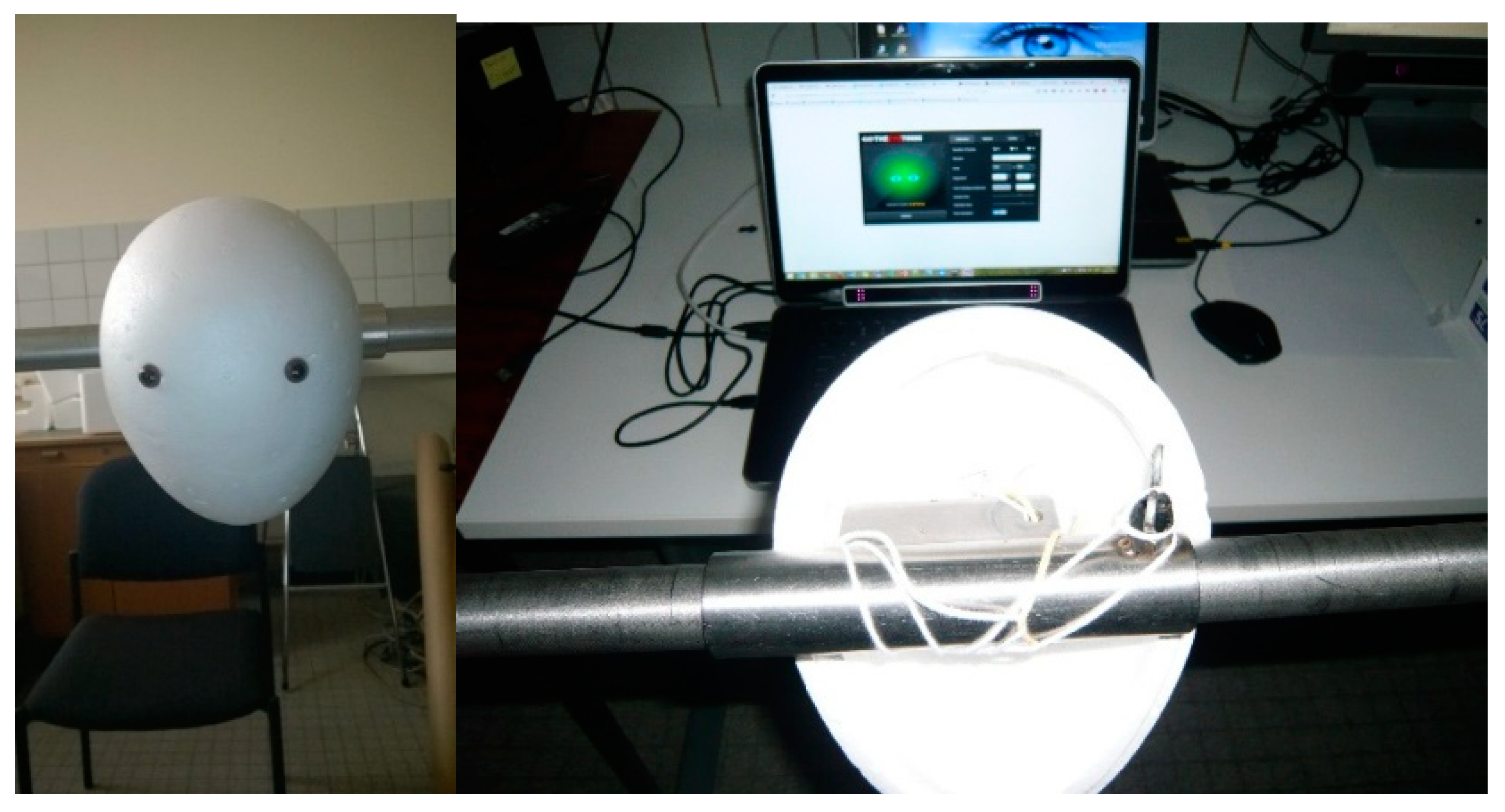
Two types of participants can be distinguished: Artificial and real participants (in short, AP and RP respectively). The AP was constructed out of a polystyrene egg shape—30 cm from top to bottom, wide side at the top—on which two artificial eyes (in glass, used for stuffed animals, 2 cm diameter) were attached. The position of the eye (on the head and mutual distance) was adjusted until the Eye Tribe UI indicated a stable detection of both artificial eyes. To guarantee a fixed position of the artificial eyes and head, the latter was attached to a horizontal bar of which both ends were placed on tripods. This distance between the artificial eyes and the screen was 60 cm. This set-up is further illustrated in Figure 1.
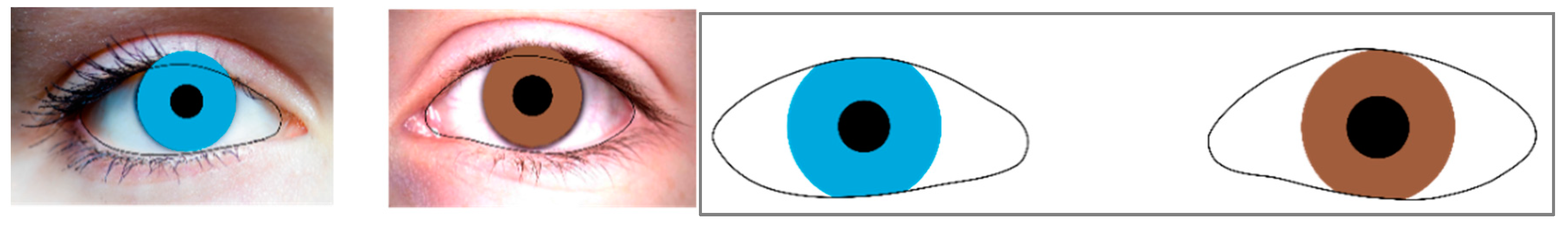
It must be noted however that the initial idea for the artificial participant was to have a set of printed artificial eye on paper based on real eyes (see Figure 2 for a sample), as in Krassanakis et al. (2016) [49]. However, the Eye Tribe UI did not detect these eyes, even when they were printed on alternative types of backgrounds (e.g., plastic to create a reflection). It was discovered that the software takes a multi-layered detection approach, similar to what is described by Gómez-Poveda and Gaudioso (2016) [21], starting with the distinction of the shape of the head. Therefore, a curved surface is required, which was approximated by the egg-shape.
Next, five real participants were invited to take part in the test. These were all employees of the Department of Geography at Ghent University who were asked to execute a simple task on the screen (see Section 3.3). These participants were seated at a distance of 60 cm from the screen. They were informed that their eyes were being monitored and that their data would be analyzed anonymously. All participants agreed to this procedure.
3.2. Apparatus
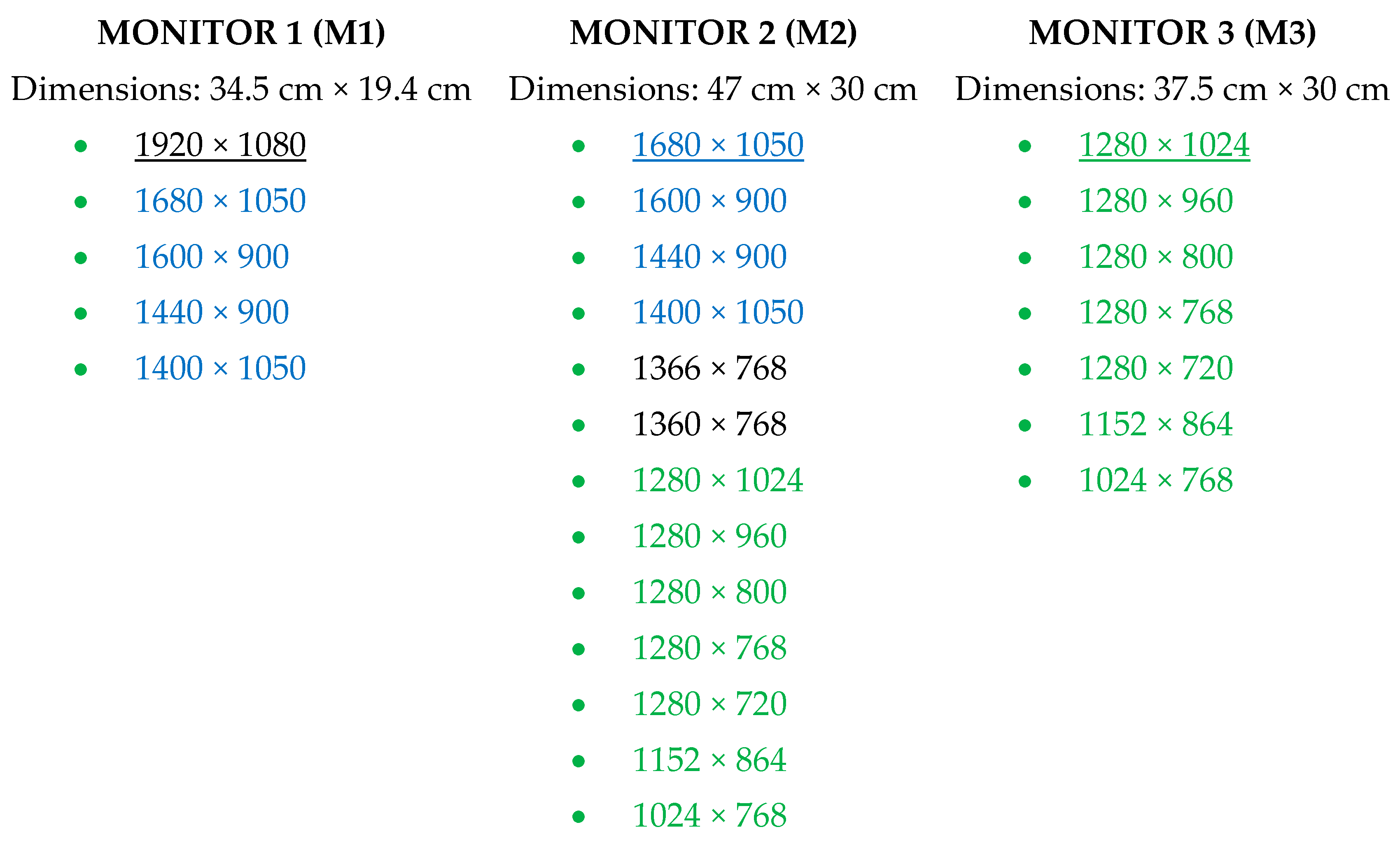
All data were registered with an Eye Tribe Tracker (see Table 1 for specifications). For the AP, the eye movements were recorded at 30 Hz and 60 Hz. Furthermore, the device was connected with three types of monitors on which different settings for the resolution were selected. An overview of the specifications of the three monitors can be found in Figure 3. The default resolution of the monitors is underlined, and the colors indicate which resolutions were available on multiple monitors. The data of the RPs was only recorded at 60 Hz, using M2 with its default resolution.
3.3. Stimuli and Tasks
With the AP no stimuli were created as the artificial eyes only gazed continuously at one fixed point. This gaze was recorded for 5 min in each trial, varying in monitor set-up (dimensions and resolution) and sampling rate of the tracker (see Section 3.2).
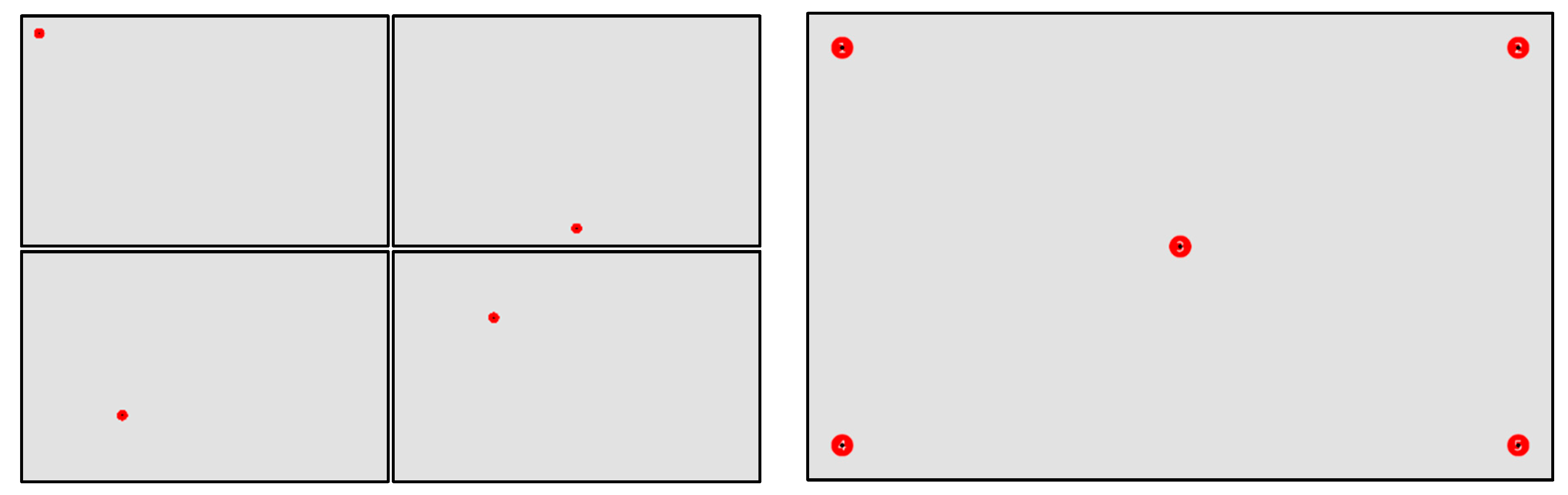
For the RPs, a set of stimuli were created which all had the same grey background (RGB = 225, 225, 225). On this background, targets were placed (see Figure 4) which constitute out of a red circle with a black dot in the center. The size of the circle (radius in pixels, R) was based on the reported accuracy of the visual angle that could be recorded by the Eye Tribe Tracker (0.5°–1.0°) and the distance between the participant and the screen (60 cm). The radius of the circle corresponds to 36.7 px and 73.3 px with visual angle of 0.5° and 1.0° respectively. Therefore, it was opted to take the rounded average in this interval, which is 50 px (corresponding to a visual angle of about 0.7°). The size of the black dot in the center is 10 px.
In total, 14 stimuli were created, from which 13 contained only one target. These latter images were displayed one by one to the participant in a random order, which was the same for all participants. Table 2 lists the coordinates of all targets (in screen coordinates). Each stimulus, and therefore each target, was displayed for five seconds and the participants were asked to fixate on the central dot in the red circle. The last image contained five targets, which were numbered (in white, see Figure 4). This stimulus remained visible for 25 s and the participants were asked to fixate each target for about five seconds.
3.4. Procedure
All tests were conducted at the Eye Tracking Laboratory of the Department of Geography at Ghent University. The eye movement data was recorded using PyTribe, a Python wrapper for the Eye Tribe tracker—based on PyGaze7—which can be downloaded from GitHub [32,71].
The tests with the AP did not require any calibration as the AP’s gaze is fixed on one point. In total 50 trials of five minutes each were recorded with the AP (25 different “monitor x resolution”-combinations and two sampling rates), which were saved in a text file. This file contains a timestamp (in ms), state (how many eyes were detected), the x and y locations of the gaze (left and right eye separately and combined, including the raw and average values) and information on the pupil (size and position).
For each of the 50 trials, the deviation (Euclidean distance between target and gaze position) was calculated expressed in pixels and in visual angle, considering a theoretical viewing distance of 50 cm, 55 cm, 60 cm, and 65 cm for the left eye, right eye, and the combined value.
The tests with the RPs were preceded by a calibration procedure—using the Eye Tribe UI—based on five calibration points. Similarly, as with the AP, all eye movements were recorded using the PyTribe code, in which the stimuli (including their timings) could be implemented.
The data is processed using different manual and automatic procedures in order to optimize its quality. The Eye Tribe Tracker provides two sets of positions—The raw positions (raw) and average (avg) positions. The latter are already initially processed by the Eye Tribe server while recording—smoothed positions. First these two data sets are manually filtered based on two criteria:
- The recordings during the first second of a trial is removed as the participant has to redirect its gaze towards the target point.
- The recordings indicated by a state “8” are removed. This corresponds to the situation where the eye tracker was unable to determine the position of the right and left eye.
Next, the data (avg and raw, both unfiltered and filtered) is further processed by applying a fixation detection which is capable of removing noise. The identification of fixation events is based on the implementation of the dispersion-based algorithm of EyeMMV toolbox [52]. This toolbox was selected because (1) it is open-source, and (2) it has the capability to filter out noise when detecting samples within the raw data. This algorithm implements both spatial and temporal criteria: The spatial dispersion threshold is implemented in two steps, while the temporal one corresponds to the minimum value of fixation duration. Hence, the execution of EyeMMV’s algorithm requires the selection of two spatial parameters. The first parameter is related to the range of central vision (i.e., the spatial dispersion of raw data during a fixation event, see also the section fixation identification algorithms and thresholds), while the second one is applied towards the verification of each fixation cluster consistency. The second spatial parameter can be based on the statistical interval of 3 s for each cluster, or to be considered as a constant value. In the first case the second parameter is adapted to each cluster separately. In the second case (the accuracy of the eye tracking device is well-known_ the second spatial parameter can be based on these reported accuracy values. A detailed description of the algorithm and its parameters can be found in Krassanakis et al. (2014) [52]. The latter study also illustrates that the use of the constant value as second parameters results in a better performance compared to the statistical interval of 3 s.
The execution of EyeMMV’s algorithm was performed only for the RPs. More specifically, considering the fixation thresholds’ values reported in the literature (see Section 2.4, on fixation identification algorithms and thresholds), the performance of the algorithm was based on the range between 0.7°–1.3°, with an interval of 0.1° for the selection of first spatial dispersion parameter. The second parameter of the algorithm will be based on the average noise calculated derived from the recordings with the AP (see Section 4.1). Additionally, the value of 80 ms (minimum reported value in the literature) was selected as the minimum fixation duration for the execution of EyeMMV’s algorithm.
Finally, the deviation of the gaze position, relative to the actual target point, is calculated for all combinations, as illustrated in Table 3.
4. Results
4.1. Artificial Participant
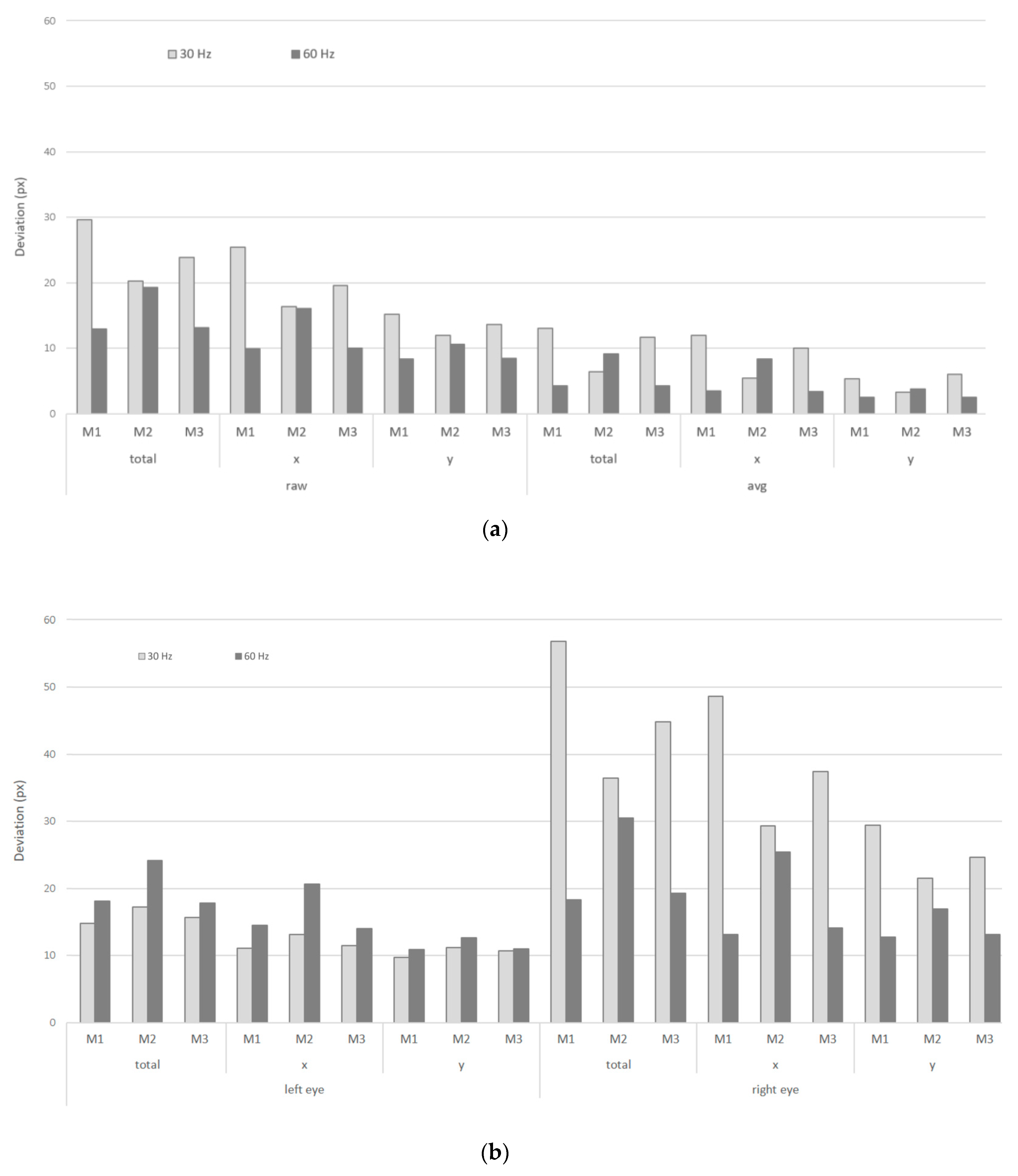
Figure 5 shows the deviations of the registered gaze locations (in pixels) from the real target locations on M1, M2, and M3 at their default resolution, recorded at 30 Hz (left), and 60 Hz (right). These give insights in the precision of the recordings. Separate values are given for (based on Eye Tribe measures): The raw and the average (smoothed) coordinates, the x and y values, and the obtained values for the left and right eye. Since we used the (unprocessed) Eye Tribe output values, the results are presented in pixels (without a recalculation to visual angle). The smoothed (avg) coordinates are also registered from the Eye Tribe’s output, without any additional modifications. However, no information from the Eye Tribe documentation is available on how these coordinates were calculated. Firstly, when considering the smoothed coordinates (avg), the value for the deviations is much lower in comparison with the raw coordinates. The obtained values for avg are in the order of 5 px and less. Secondly, a larger deviation can be noted in the y-coordinates, although the y-dimension of the monitor is smaller than the x-dimension. Thirdly, a variation between the deviations for the left and right eye can be noted. Finally, better results are obtained when a sampling rate of 60 Hz is used compare to the 30 Hz recordings in this specific set-up.
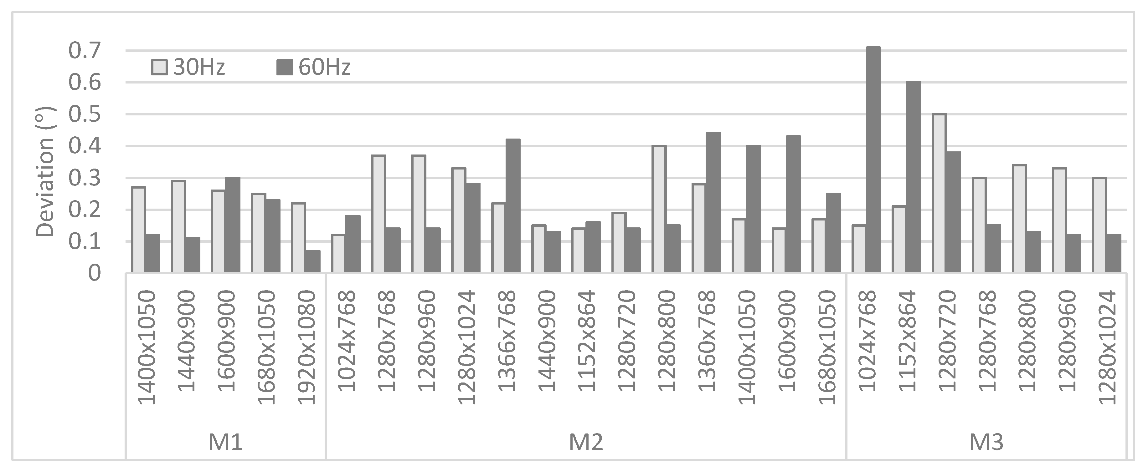
The obtained deviations are recalculated in terms of visual angle, which is dependent on the viewing distance. Besides the 60 cm distance that was employed during the experiment, deviations corresponding to three other (theoretical) viewing distances are calculated as well—50 cm, 55 cm, and 65 cm. The results can be found in Figure 6, with a distinction between the 30 Hz and 60 Hz recordings for M1 at different resolutions.
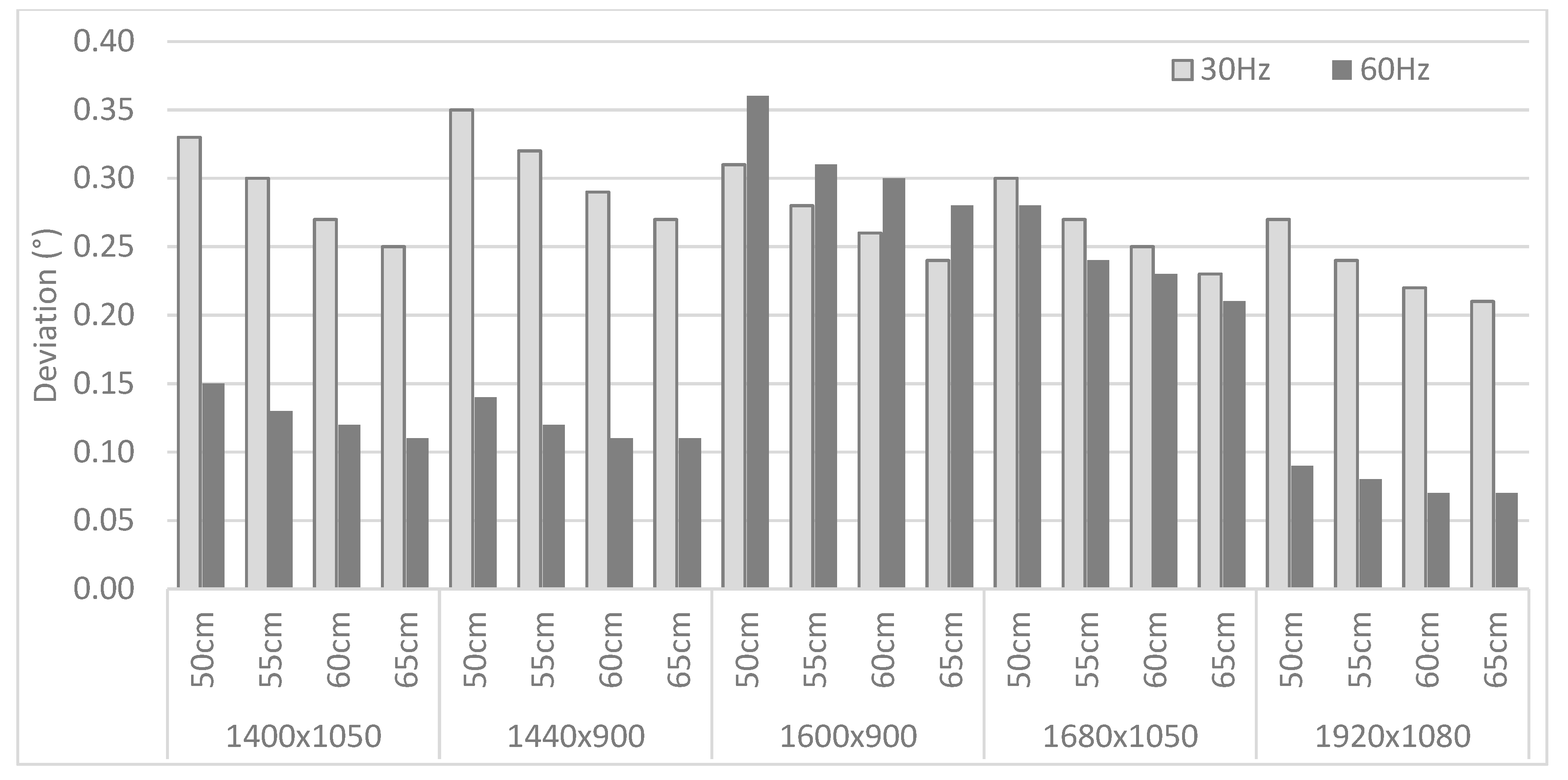
Figure 7 focuses on the different monitors and their resolutions, listing the deviations (expressed in visual angle) for the recordings at 30 Hz and 60 Hz at a viewing distance of 60 cm. The obtained values range between 0.1° to 0.7° (with an average of 0.25°), which is conform the accuracy values provided by the vendor. No clear trend in the deviations is found when considering the different sampling rates or monitors and their resolutions.
4.2. Real Participants
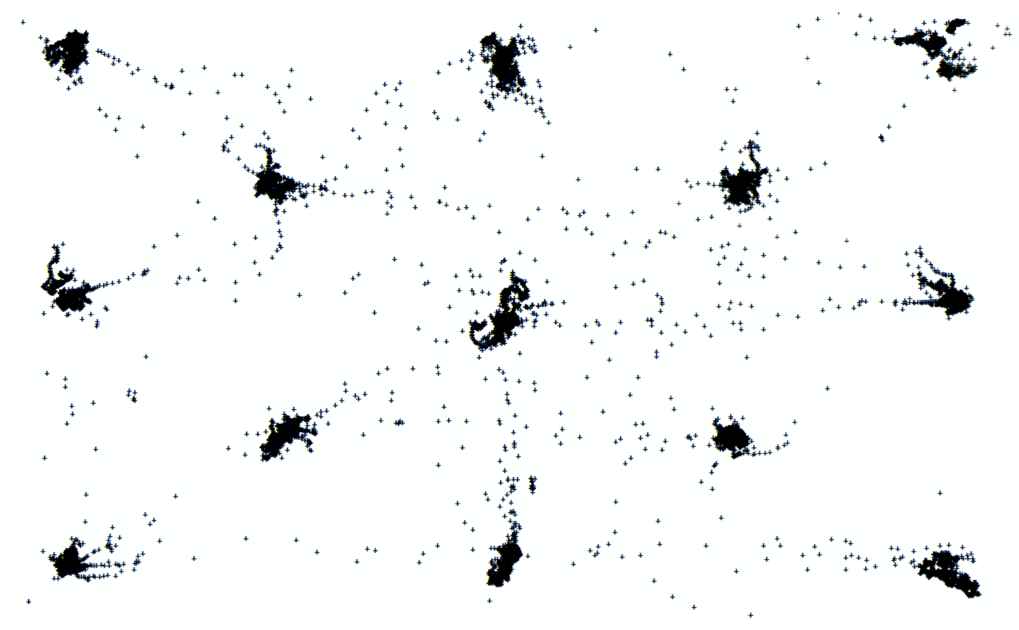
In contrast with the AP, the RPs fixated multiple target points. Two different types of stimuli (separate target points or a combined set of target points) were implemented to allow evaluating their influence on the registered eye tracking data. Firstly, the 13 points were displayed separately which means that only one point was visible for a fixed amount of time (of five seconds). Only the data registered in a specific time interval was assigned to the corresponding target point. Figure 8 shows the registered raw data for the 13 target points that were displayed on after the other. Secondly, the five points were displayed together in one image and the participant had to move from one point to the next on his/her own initiative. This was included as an extension on the study, as this is a more top-down processing-oriented task, which can have a severe impact on how participants focus or get distracted (e.g., Reference [72]). For this part of the study, we had to assign the gaze data to its corresponding target. This can be done easily based on the fixed order with which these targets were fixated and a fixed distance around each target point. This approach is similar to the results obtained when the 13 points were displayed separately.
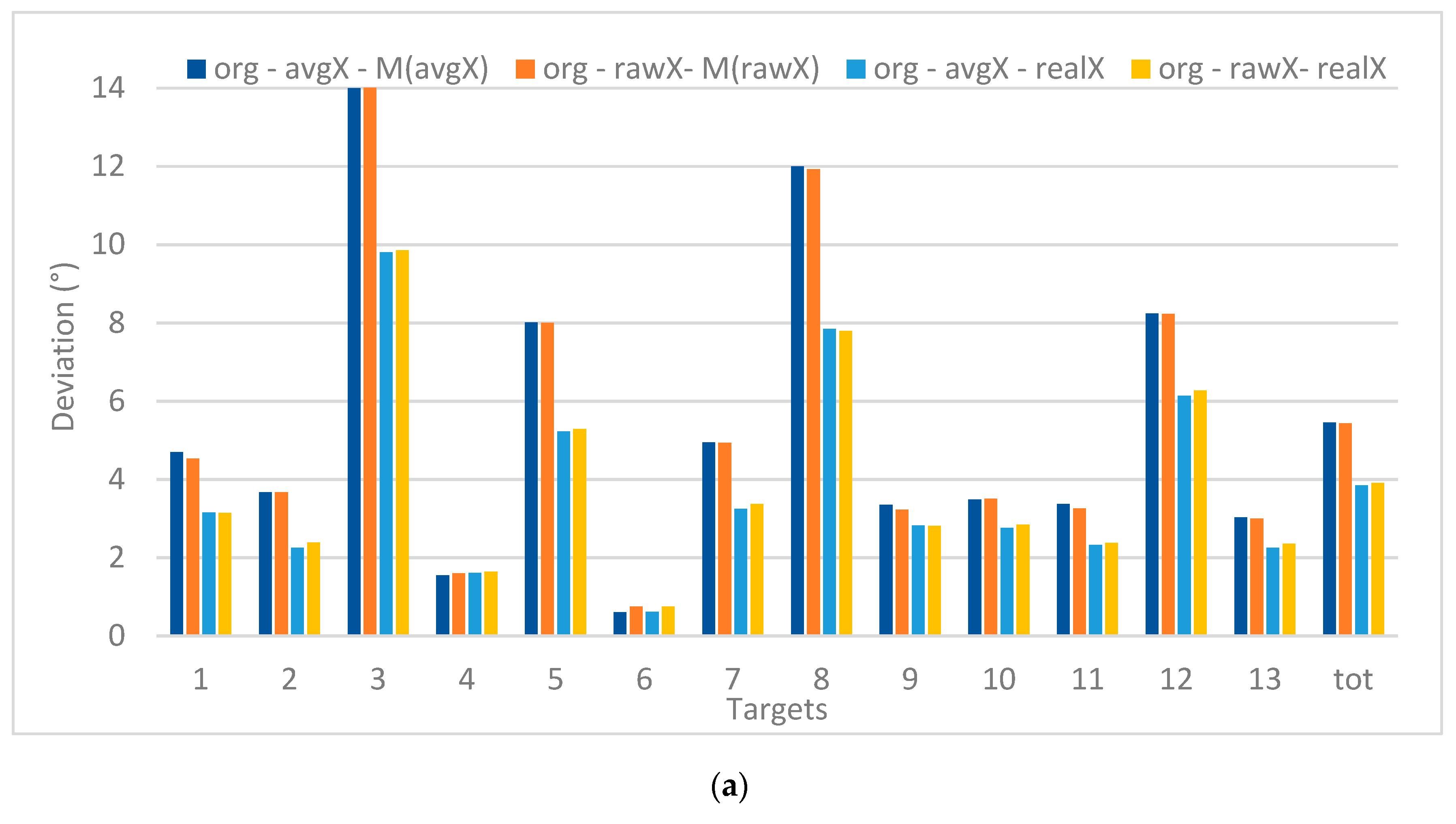
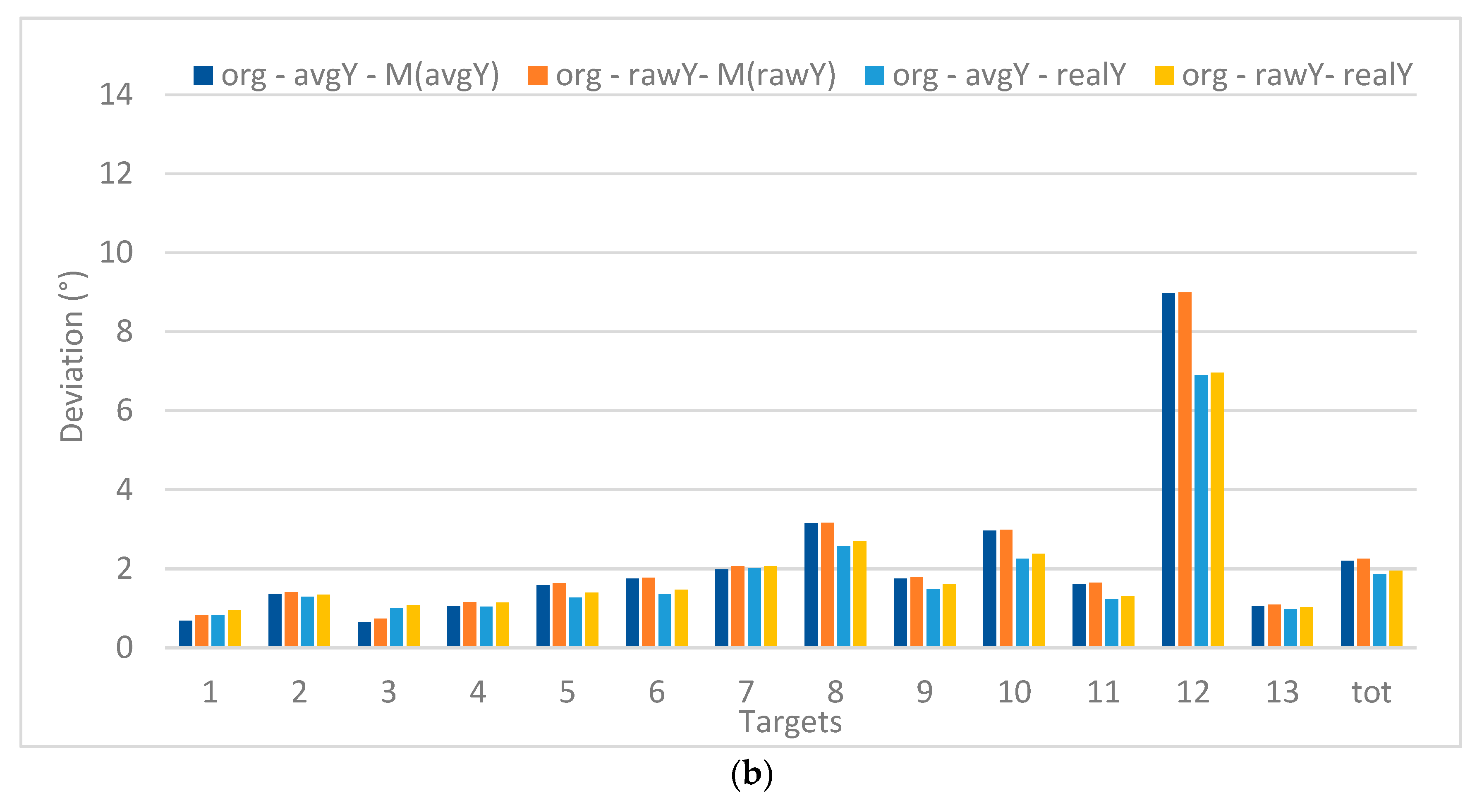
Figure 9 shows the deviations (expressed in visual angle, at a viewing distance of 60 cm) for each of the target points when processing the original gaze data (13 targets) in X (left) and Y (right). The values are, on the one hand, compared to the real X and Y positions of the targets and, on the other hand, to the mean value of the recorded X and Y positions (M(avgX) or M(avgY)). This way it can be discovered if there is a systematic deviation between the recorded values and the real values, which allows comparing precision versus accuracy. Furthermore, the raw versus avg data sets (both unfiltered) are considered. The graphs clearly indicate that a smaller deviation is registered when comparing to the real target position (related to precision) instead of the mean position values (related accuracy). Furthermore, the deviations are larger in the X than in Y.
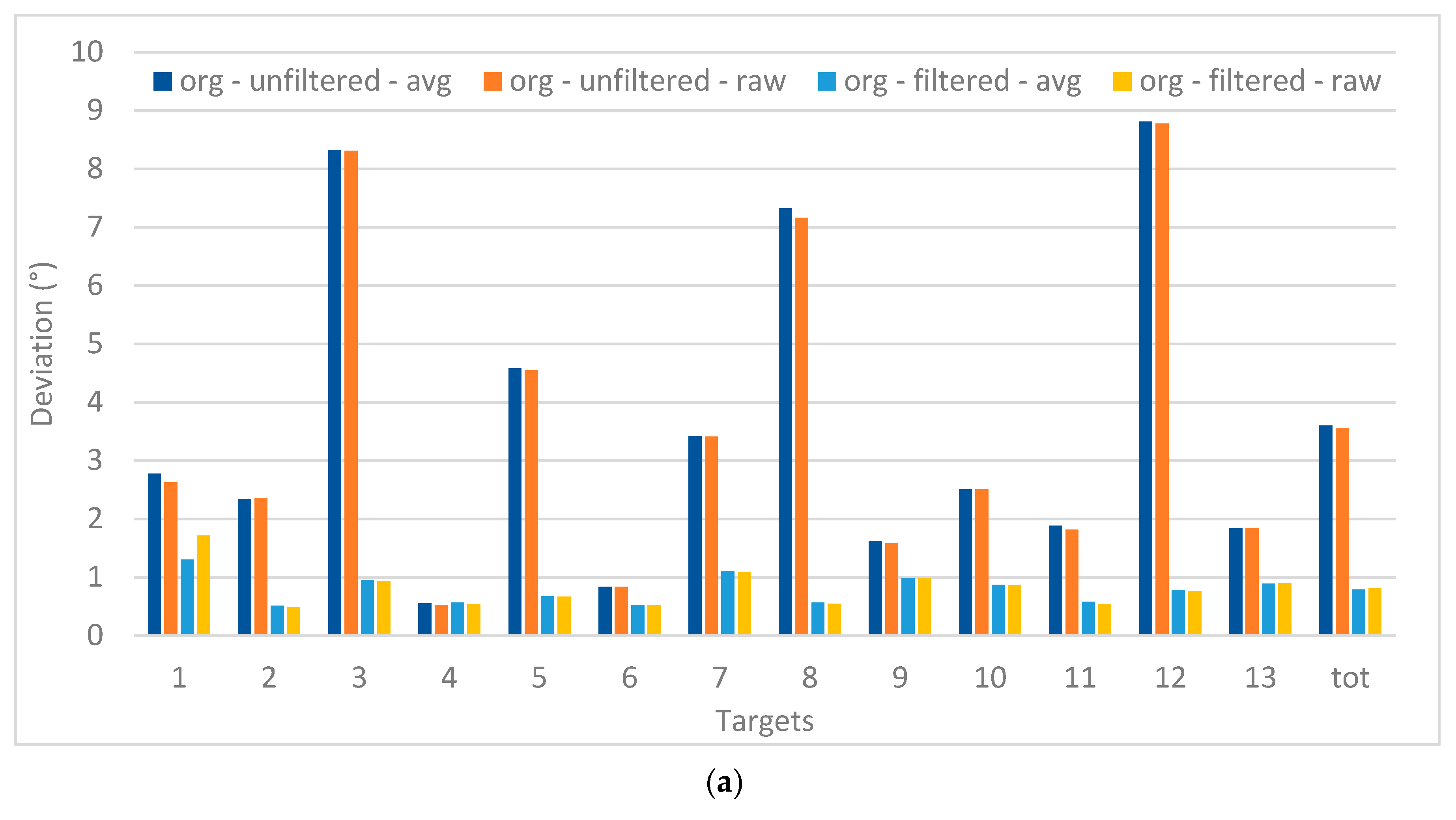
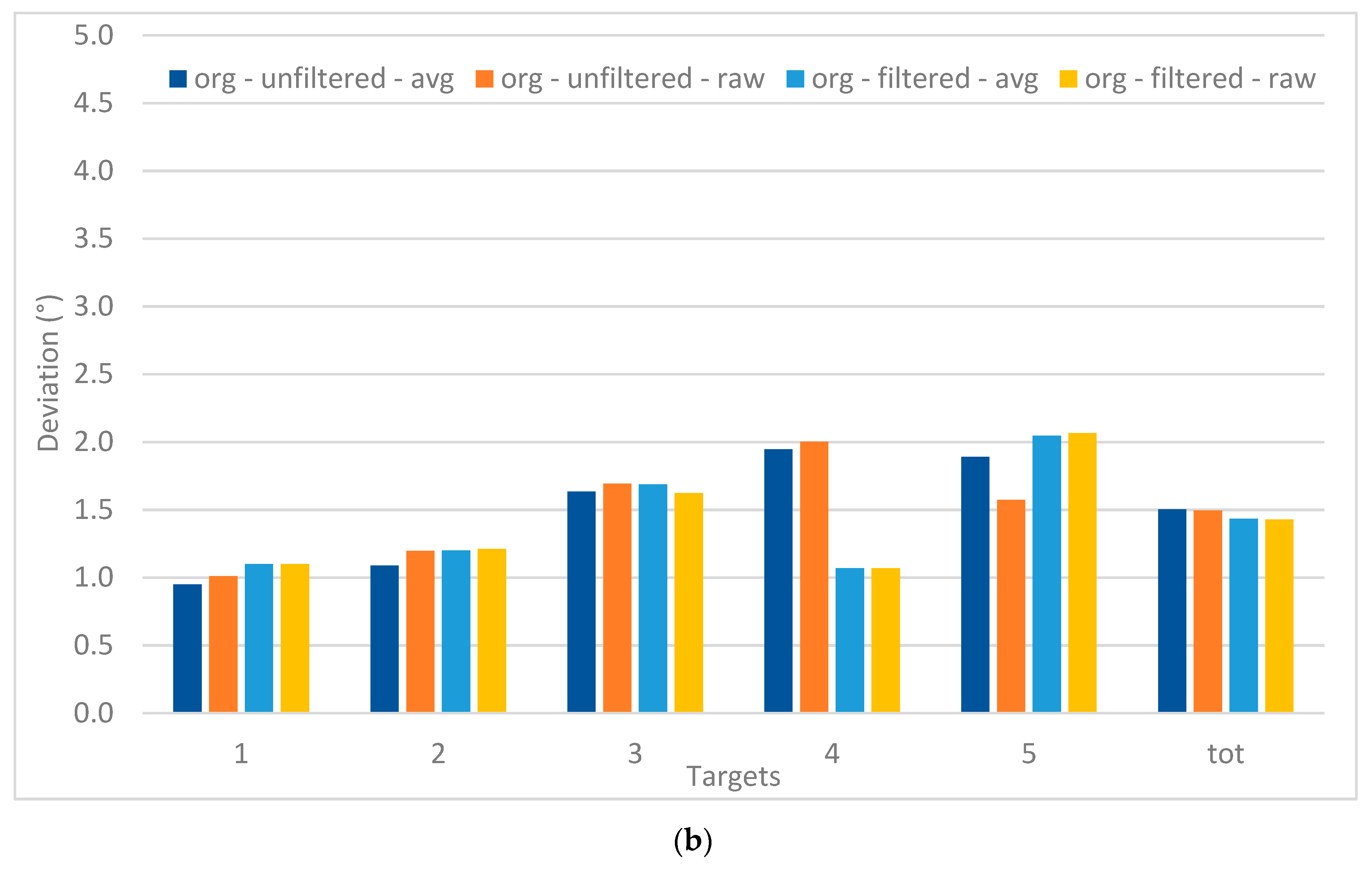
Figure 10 focusses on the deviations for each of the target position, compared to their real position. For the 13 targets, a large difference between the filtered and unfiltered data is apparent, which is not the case for the data when there were five targets. This is also confirmed by the Univariate ANOVA test presented in Table 4, which also shows the interaction effect between filtering and the type of target. Although the overall values for the five-target stimuli are much lower, no significant difference is found. The difference between the avg and raw values is also not found to be significant.
Besides the manual filtering, the application of EyeMMV’s fixation detection algorithm (which is described in Section 3.4) also includes a noise reducing component. This procedure is—next to the manual filtering—thus an alternative option to remove noise and at the same time aggregate the data. Besides the seven spatial dispersion thresholds: 0.7°, 0.8°, 0.9°, 1.0°, 1.1°, 1.2°, and 1.3°. The value for the average noise was set to 0.25° (derived from the AP recordings, see before). In other words, for the execution of the algorithm considering the spatial threshold dispersion 1.0°, the values delineating the average noise correspond to t1 = 1.25°, and t2 = 1.0°.
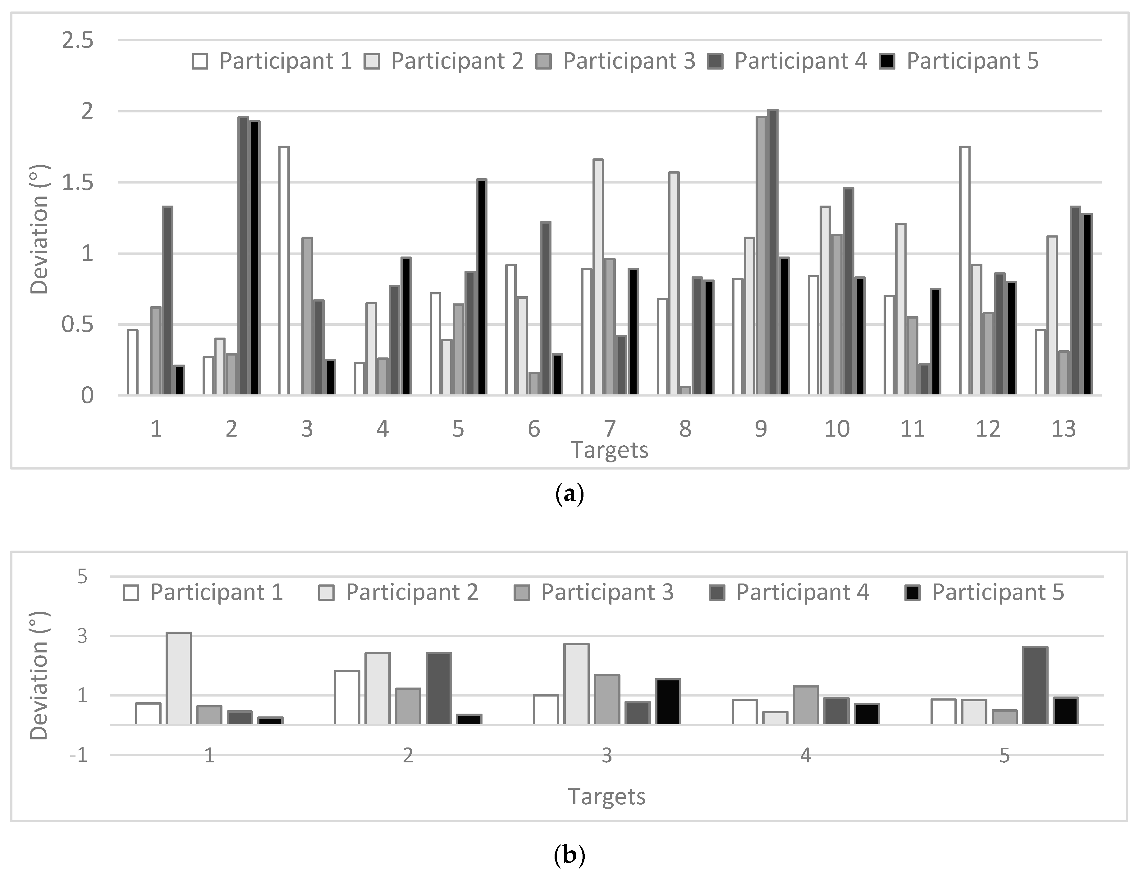
The extraction of fixations (and their position) allows calculating deviations from the actual location of the targets. For example, for the case of the average threshold of 1.0°, the resulting values for these deviations in the avg unfiltered data set are, for each participant, presented in Figure 11a for the 13 target points—and in Figure 11b for the five target points.
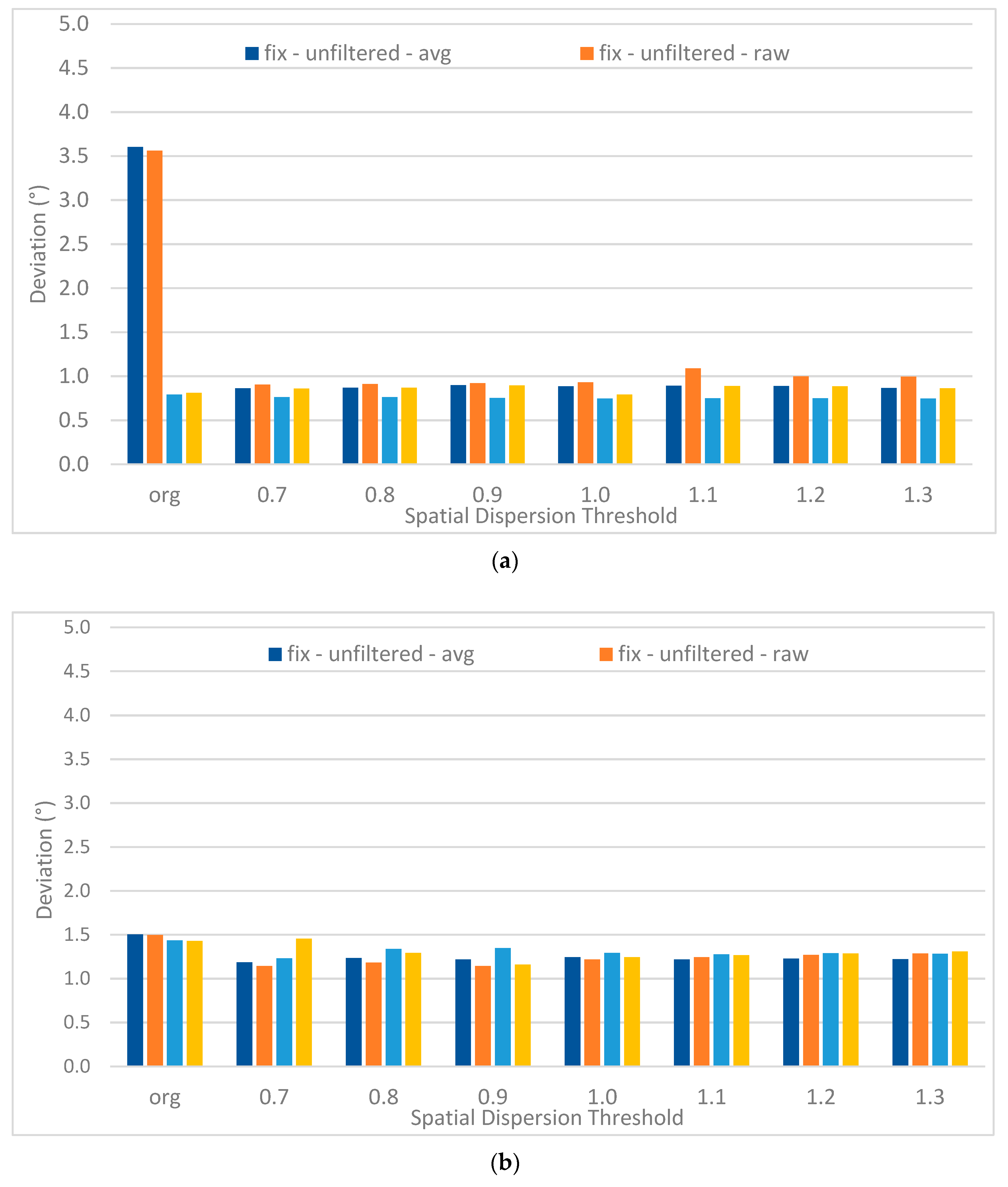
EyeMMV’s algorithm allows defining spatial parameters in order to filter out the noise in the data. The results for the parameters ranging from 0.7 to 1.3 are presented in Figure 12 and compared with the original data before the application of the fixation detection algorithm (filtered or not). Overall, it can be noticed that the deviations are somewhat higher for the 5 target points. The associated statistical analysis (based on repeated measures, see Table 5) reveal the variation in the deviations is significant for the 13 target points when applying the fixation detection algorithm on the unfiltered data. The raw data for the 13 target points also shows a significant improvement when applying the algorithm after filtering, which is not the case for the avg data set. Overall after applying the fixation detection algorithm, the deviations are somewhat higher for the five-point targets compared to these of the 13 targets.
5. Discussion
The execution of visual experimentation based on low-cost and/or no-cost (e.g., ordinary webcams) devices constitutes one of the most challenging topics in the field of eye tracking. Despite the fact that these types of devices may be quite suitable for basic needs of HCI, such as software interface manipulation through the eyes of the user, the question about the use of these devices in scientific research still remains. The experimental set-up presented in the current study contributes to the state of the art in the field, by delivering representative results of spatial noise measurements for the case of the low-cost Eye Tribe eye tracker. This may serve as a guide for future studies. These results can be used as input for the execution of EyeMMV’s algorithm, which uses a “two-step” spatial dispersion threshold for fixations identification, considering the spatial noise of the eye tracker as input to the algorithm.
The performance of the low-cost device is evaluated with both artificial and real participants, taking into account different settings. With the AP different monitor settings (dimensions and resolutions), eye tracker frequencies and (theoretical) viewing distances were implemented. The recorded deviations (Figure 6) show lower (and thus better) results when recorded at a sampling rate of 60 Hz. However, the difference with 30 Hz is in the order of 0.2° or less. Nevertheless, a difference is found between the recordings from the left and right eye. Although this cannot be confirmed, it could be explained by the orientation of the artificial head and eyes or the even the quality of the eyes itself. Furthermore, the effect of the different viewing distances is clearly present, with a decreasing deviation in case of an increasing viewing distance. Moreover, the obtained values produced from the use of different monitor set-ups (Figure 7) range between 0.1° to 0.7° (with an average of 0.25°) which is conform the accuracy values provided by the vendor. No clear trend in the deviations is found when considering the different sampling rates or monitors and their resolutions.
The recordings for the RP were verified according to their precision (deviation from the real target position) and accuracy (clustering of the recordings or deviation from the average location). The results show a consistently better value regarding precision than accuracy. The deviations in accuracy where especially higher in the X-direction compared to the Y-direction. This latter finding can (only partially) be explained by the fact that the monitor’s dimensions are larger in X compared to Y.
The manual filtering step, based on a few simple criteria, already significantly improved the precision of the data to an average of less than 1° for the 13 point targets and around 1.5° for the 5 point targets. However, in the latter case, the effect of the manual filtering step is limited as the unfiltered data already showed smaller deviating values.
The application of the EyeMMV’s fixation detection algorithm also implies a noise filtering step. Taking the results of deviations for the case of threshold 1.0° for 13 targets (Figure 9a) and five targets (Figure 9b) as an example, it is clear that the obtained values are higher compared to those of the AP, with an average value of respectively 0.88° and 1.24°. However, no clear trend related to the position of the target points can be distinguished.
The application of the EyeMMV’s fixation detection algorithm (different thresholds) show a significant improvement in the recorded deviations for the 13 targets, when it is applied on the unfiltered data set. However, the improvement when applying EyeMMV’s algorithm on the data set which was already manually filtered is only significant in one case (13 point, raw data). A smaller improvement after the application of the EyeMMV’s algorithm can be seen in the graph showing data for five targets, but this is not found to be significant. Nevertheless, no significant difference is found with the application of the different spatial thresholds integrated in the EyeMMV’s algorithm. The range of these thresholds (0.7–1.3) was already based on the modelled noise from the AP, which can explain the limited variation within them.
Additionally, the results which correspond to the average difference values of all tested thresholds indicate that the final coordinates of the original recordings or fixation events may be comparable with corresponded values produced in expensive devices, respectively after manual filtering or the performance of EyeMMV’s algorithm. What is more, the 13 point stimuli’s correspond to a standard calibration procedure (with possibly less target points), which could be employed as such in future studies to verify the precision and accuracy of the recordings during an experiment. However, the results highlight slightly higher deviations for the case of five targets (multi-task-oriented observation). This can be explained by the fact that this task corresponds more to top-down processing comparted to bottom-up processing (in the case of the separate 13 targets) [72].
EyeMMV’s algorithm could also be evaluated using as second spatial threshold a value connected with the std (to be more precise the statistical threshold of 3 s). This was not implemented in the research because it was indicated in by Krassanakis et al., 2014 [52] that the performance was better when using a constant value. However, it could be useful to investigate how the values differ based on these different filtering techniques.
The results of the present study are in correspondence with the conclusion produced by a previous study presented by Ooms et al. (2015) [26], and indicate that the low-cost devices can be used for the performance of scientific research after the optimal selection of the experimental set-up. Except from that the present study reports critical values of spatial noise produced in several set-ups, it indicates the way to effectively use these values as an input in EyeMMV’s fixation identification algorithm.
6. Conclusions & Future Work
An integrated methodological framework is presented through the current study towards the measurement of the spatial noise produced in eye tracking devices. Initially the noise is modelled using the artificial participant, which gazes continuously on a single point in space. Deviations from this location are caused by noise, which is measured in the experiment. Next experiments are executed with ‘real’ test persons who have to focus on different target points on the screen. Two alternative approaches are proposed to reduce the noise in the data: The application of a manual filtering step and the application of a fixation detection algorithm (from EyeMMV) in which noise reduction parameters are implemented. A significant improvement is found for both approaches when different targets are fixated separately. Consequently, if the aim is to further analyze the aggregated data (which requires the need for the application of a fixation detection algorithm), the EyeMMV’s algorithm can be applied directly as it can filter out the noise while aggregating the data. If the original gaze data is required, a simple manual filtering step already suffices to significantly improve the quality of the recorded data. The outcomes show that the use of low-cost devices is feasible and may produce valuable results for further analysis (metrics computations, eye tracking visualizations, etc.). Furthermore, other filtering techniques (simple and more complex) could be evaluated as well to process the obtained data.
Despite the fact that the presented research study is based on a low-cost device, this framework (including a low-cost set-up with artificial eyes) can be implemented in any eye tracker. A challenging process is to measure the corresponded values of spatial noise and to use the same algorithm in order to compute fixations from gazes produced from ordinary webcam and/or work with simple software (such as a web browser). What is more, this study was conducted in a controlled laboratory set-up. It would be also be useful to get insights in the performance of these low-cost eye trackers in less optimal conditions (e.g., variation in the light source, more dynamic stimuli, changing tasks). Other algorithms have already been developed to deal with adaptation issues in these changing conditions [73,74,75].
Author Contributions
Conceptualization, K.O. and V.K.; Formal analysis, K.O. and V.K.; Investigation, K.O. and V.K.; Methodology, K.O. and V.K.; Software, V.K.; Validation, K.O. and V.K.; Visualization, K.O.; Writing—original draft, K.O. and V.K.; Writing—review & editing, K.O. and V.K.
Funding
This research received no external funding.
Conflicts of Interest
The authors declare no conflicts of interest.
References
- Mele, M.L.; Federici, S. Gaze and eye-tracking solutions for psychological research. Cognit. Process. 2012, 13, 261–265. [Google Scholar] [CrossRef] [PubMed]
- Sharma, A.; Abrol, P. Eye Gaze Techniques for Human Computer Interaction: A Research Survey. Int. J. Comput. Appl. 2013, 71. [Google Scholar] [CrossRef]
- Poole, A.; Ball, L.J. Eye tracking in HCI and usability research: Current Status and Future Prospects. In Encyclopedia of Human Computer Interaction; Ghaoudi, C., Ed.; Idea Group: Pennsylvania, PA, USA, 2005; pp. 211–219. [Google Scholar]
- Rosch, J.L.; Vogel-Walcutt, J.J. A review of eye-tracking applications as tools for training. Cognit. Technol. Work 2013, 15, 313–327. [Google Scholar] [CrossRef]
- Lai, M.L.; Tsai, M.J.; Yang, F.Y.; Hsu, C.Y.; Liu, T.C.; Lee, S.W.Y.; Lee, M.H.; Chiou, G.L.; Liang, J.C.; Tsai, C.C. A review of using eye-tracking technology in exploring learning from 2000 to 2012. Educ. Res. Rev. 2013, 10, 90–115. [Google Scholar] [CrossRef]
- Wedel, M.; Pieters, R. A review of eye-tracking research in marketing. Rev. Market. Res. 2008, 4, 123–147. [Google Scholar]
- Clifton, C.; Ferreira, F.; Henderson, J.M.; Inhoff, A.W.; Liversedge, S.P.; Reichle, E.D.; Schotter, E.R. Eye movements in reading and information processing: Keith Rayner’s 40year legacy. J. Mem. Lang. 2016, 86, 1–19. [Google Scholar] [CrossRef]
- Buswell, G.T. How People Look at Pictures; University of Chicago Press: Chicago, IL, USA, 1935. [Google Scholar]
- Yarbus, A.L. Eye Movements and Vision; Plenum Press: New York, NY, USA, 1967. [Google Scholar]
- Nyström, M.; Holmqvist, K. An adaptive algorithm for fixation, saccade, and glissade detection in eyetracking data. Behav. Res. Methods 2010, 42, 188–204. [Google Scholar] [CrossRef] [PubMed]
- Mould, M.S.; Foster, D.H.; Amano, K.; Oakley, J.P. A simple nonparametric method for classifying eye fixations. Vis. Res. 2012, 57, 18–25. [Google Scholar] [CrossRef] [PubMed]
- Krassanakis, V.; Filippakopoulou, V.; Nakos, B. EyeMMV toolbox: An eye movement post-analysis tool based on a two-step spatial dispersion threshold for fixation identification. J. Eye Mov. Res. 2014, 7, 1–10. [Google Scholar]
- Larsson, L.; Nyström, M.; Andersson, R.; Stridh, M. Detection of fixations and smooth pursuit movements in high-speed eye-tracking data. Biomed. Signal Process. Control 2015, 18, 145–152. [Google Scholar] [CrossRef]
- Gitelman, D.R. ILAB: A program for postexperimental eye movement analysis. Behav. Res. Methods Instrum. Comput. 2002, 34, 605–612. [Google Scholar] [CrossRef] [PubMed] [Green Version]
- Voßkühler, A.; Nordmeier, V.; Kuchinke, L.; Jacobs, A.M. OGAMA (Open Gaze and Mouse Analyzer): Open-source software designed to analyze eye and mouse movements in slideshow study designs. Behav. Res. Methods 2008, 40, 1150–1162. [Google Scholar] [CrossRef] [PubMed] [Green Version]
- Berger, C.; Winkels, M.; Lischke, A.; Höppner, J. GazeAlyze: A MATLAB toolbox for the analysis of eye movement data. Behav. Res. Methods 2012, 44, 404–419. [Google Scholar] [CrossRef] [PubMed]
- Zhegallo, A.V.; Marmalyuk, P.A. ETRAN—R Extension Package for Eye Tracking Results Analysis. Perception 2015, 44, 1129–1135. [Google Scholar] [CrossRef] [PubMed]
- Camilli, M.; Nacchia, R.; Terenzi, M.; Di Nocera, F. ASTEF: A simple tool for examining fixations. Behav. Res. Methods 2008, 40, 373–382. [Google Scholar] [CrossRef] [PubMed] [Green Version]
- Di Nocera, F.; Capobianco, C.; Mastrangelo, S. A Simple (r) Tool for Examining Fixations. J. Eye Mov. Res. 2016, 9, 1–6. [Google Scholar]
- Xu, P.; Ehinger, K.A.; Zhang, Y.; Finkelstein, A.; Kulkarni, S.R.; Xiao, J. TurkerGaze: Crowdsourcing saliency with webcam based eye tracking. arXiv, 2015; arXiv:1504.06755. [Google Scholar]
- Gómez-Poveda, J.; Gaudioso, E. Evaluation of temporal stability of eye tracking algorithms using webcams. Expert Syst. Appl. 2016, 64, 69–83. [Google Scholar] [CrossRef]
- Papoutsaki, A.; Daskalova, N.; Sangkloy, P.; Huang, J.; Laskey, J.; Hays, J. WebGazer: Scalable Webcam Eye Tracking Using User Interactions. In Proceedings of the 25th International Joint Conference on Artificial Intelligence (IJCAI), New York, NY, USA, 9–15 July 2016; pp. 3839–3845. [Google Scholar]
- Ferhat, O.; Vilariño, F.; Sanchez, F.J. A cheap portable eye-tracker solution for common setups. J. Eye Mov. Res. 2014, 7, 1–10. [Google Scholar]
- Skodras, E.; Kanas, V.G.; Fakotakis, N. On visual gaze tracking based on a single low cost camera. Signal Process. Image Commun. 2015, 36, 29–42. [Google Scholar] [CrossRef]
- Parada, F.J.; Wyatte, D.; Yu, C.; Akavipat, R.; Emerick, B.; Busey, T. ExpertEyes: Open-source, high-definition eyetracking. Behav. Res. Methods 2015, 47, 73–84. [Google Scholar] [CrossRef] [PubMed]
- Ooms, K.; Dupont, L.; Lapon, L.; Popelka, S. Accuracy and precision of fixation locations recorded with the low-cost Eye Tribe tracker in different experimental set-ups. J. Eye Mov. Res. 2015, 8, 17–26. [Google Scholar]
- Ferhat, O.; Vilariño, F. Low Cost Eye Tracking: The Current Panorama. Comput. Intell. Neurosci. 2016, 2016, 8680541. [Google Scholar] [CrossRef] [PubMed]
- Kasprowski, P.; Harezlak, K. Using non-calibrated eye movement data to enhance human computer interfaces. In Intelligent Decision Technologies; Springer International Publishing: Berlin/Heidelberg, Germany, 2016; pp. 347–356. [Google Scholar]
- Rodrigue, M.; Son, J.; Giesbrecht, B.; Turk, M.; Höllerer, T. Spatio-Temporal Detection of Divided Attention in Reading Applications Using EEG and Eye Tracking. In Proceedings of the 20th International Conference on Intelligent User Interfaces, Atlanta, GA, USA, 29 March–1 April 2015; pp. 121–125. [Google Scholar]
- Kim, J.; Thomas, P.; Sankaranarayana, R.; Gedeon, T.; Yoon, H.J. Understanding eye movements on mobile devices for better presentation of search results. J. Assoc. Inf. Sci. Technol. 2016, 66, 526–544. [Google Scholar] [CrossRef]
- Rajanna, V.; Hammond, T. GAWSCHI: Gaze-augmented, wearable-supplemented computer-human interaction. In Proceedings of the Ninth Biennial ACM Symposium on Eye Tracking Research & Applications, Charleston, SC, USA, 14–17 March 2016; pp. 233–236. [Google Scholar]
- Dalmaijer, E. Is the low-cost EyeTribe eye tracker any good for research? (No. e585v1). PeerJ PrePrints 2014, 2, e585v1. [Google Scholar]
- Popelka, S.; Stachoň, Z.; Šašinka, Č.; Doležalová, J. EyeTribe Tracker Data Accuracy Evaluation and Its Interconnection with Hypothesis Software for Cartographic Purposes. Comput. Intell. Neurosci. 2016, 2016, 9172506. [Google Scholar] [CrossRef] [PubMed]
- Bækgaard, P.; Petersen, M.K.; Larsen, J.E. Thinking outside of the box or enjoying your 2 seconds of frame? In Proceedings of the International Conference on Universal Access in Human-Computer Interaction, Los Angeles, CA, USA, 2–7 August 2015.
- Brennan, C.; McCullagh, P.; Lightbody, G.; Galway, L.; Feuser, D.; González, J.L.; Martin, S. Accessing Tele-Services using a Hybrid BCI Approach. In Proceedings of the International Work-Conference on Artificial Neural Networks, Palma de Mallorca, Spain, 10–12 June 2015. [Google Scholar]
- Li, D.; Babcock, J.; Parkhurst, D.J. OpenEyes: A Low-cost head-mounted eye-tracking solution. In Proceedings of the 2006 Symposium on Eye Tracking Research & Applications, San Diego, CA, USA, 27–29 March 2006. [Google Scholar]
- San Agustin, J.; Skovsgaard, H.; Mollenbach, E.; Barret, M.; Tall, M.; Hansen, D.W.; Hansen, J.P. Evaluation of a low-cost open-source gaze tracker. In Proceedings of the 2010 Symposium on Eye-Tracking Research & Applications, Santa Barbara, CA, USA, 28–30 March 2010. [Google Scholar]
- Semmelmann, K.; Weigelt, S. Online webcam-based eye tracking in cognitive science: A first look. Behav. Res. Methods 2018, 50, 451–465. [Google Scholar] [CrossRef] [PubMed]
- Cheng, S.; Sun, Z.; Ma, X.; Forlizzi, J.L.; Hudson, S.E.; Dey, A. Social Eye Tracking: Gaze Recall with Online Crowds. In Proceedings of the 18th ACM Conference on Computer Supported Cooperative Work & Social Computing, Vancouver, BC, Canada, 14–18 March 2015. [Google Scholar]
- Holmqvist, K.; Nyström, M.; Andersson, R.; Dewhurst, R.; Jarodzka, H.; Van de Weijer, J. Eye Tracking: A Comprehensive Guide to Methods and Measures; Oxford University Press: Oxford, UK, 2011. [Google Scholar]
- Holmqvist, K.; Nyström, M.; Mulvey, F. Eye tracker data quality: What it is and how to measure it. In Proceedings of the Symposium on Eye Tracking Research and Applications, Santa Barbara, CA, USA, 28–30 March 2012; pp. 45–52. [Google Scholar]
- Nyström, M.; Andersson, R.; Holmqvist, K.; Van De Weijer, J. The influence of calibration method and eye physiology on eyetracking data quality. Behav. Res. Methods 2013, 45, 272–288. [Google Scholar] [CrossRef] [PubMed]
- Blignaut, P.; Wium, D. Eye-tracking data quality as affected by ethnicity and experimental design. Behav. Res. Methods 2014, 46, 67–80. [Google Scholar] [CrossRef] [PubMed]
- Hessels, R.S.; Andersson, R.; Hooge, I.T.; Nyström, M.; Kemner, C. Consequences of Eye Color, Positioning, and Head Movement for Eye-Tracking Data Quality in Infant Research. Infancy 2015, 20, 601–633. [Google Scholar] [CrossRef]
- Clemotte, A.; Velasco, M.A.; Torricelli, D.; Raya, R.; Ceres, R. Accuracy and precision of the Tobii X2-30 eye-tracking under non ideal conditions. In Proceedings of the International Congress on Neurotechnology, Electronics and Informatics (NEUROTECHNIX 2014), Roma, Italy, 25–26 October 2014. [Google Scholar]
- Mantiuk, R. Accuracy of High-End and Self-build Eye-Tracking Systems. In International Multi-Conference on Advanced Computer Systems; Springer International Publishing: Berlin/Heidelberg, Germany, 2016; pp. 216–227. [Google Scholar]
- Gibaldi, A.; Vanegas, M.; Bex, P.J.; Maiello, G. Evaluation of the Tobii EyeX Eye Tracking controller and Matlab toolkit for research. Behav. Res. Methods 2017, 49, 923–946. [Google Scholar] [CrossRef] [PubMed]
- Reingold, E.M. Eye tracking research and technology: Towards objective measurement of data quality. Vis. Cognit. 2014, 22, 635–652. [Google Scholar] [CrossRef] [PubMed] [Green Version]
- Krassanakis, V.; Filippakopoulou, V.; Nakos, B. Detection of moving point symbols on cartographic backgrounds. J. Eye Mov. Res. 2016, 9, 1–16. [Google Scholar]
- Krassanakis, V.; Filippakopoulou, V.; Nakos, B. An Application of Eye Tracking Methodology in Cartographic Research. In Proceedings of the Eye-TrackBehavior 2011(Tobii), Frankfurt, Germany, 4–5 October 2011. [Google Scholar]
- Krassanakis, V.; Lelli, A.; Lokka, I.E.; Filippakopoulou, V.; Nakos, B. Investigating dynamic variables with eye movement analysis. In Proceedings of the 26th International Cartographic Association Conference, Dresden, Germany, 25–30 August 2013. [Google Scholar]
- Krassanakis, V. Development of a Methodology of Eye Movement Analysis for the Study of Visual Perception in Animated Maps. Ph.D. Thesis, School of Rural and Surveying Engineering, National Technical University of Athens, Athens, Greece, 2014. (In Greek). [Google Scholar]
- Krassanakis, V. Recording the Trace of Visual Search: A Research Method of the Selectivity of Hole as Basic Shape Characteristic. Diploma Thesis, School of Rural and Surveying Engineering, National Technical University of Athens, Athens, Greece, 2009. (In Greek). [Google Scholar]
- Hermens, F. Dummy eye measurements of microsaccades: Testing the influence of system noise and head movements on microsaccade detection in a popular video-based eye tracker. J. Eye Mov. Res. 2015, 8, 1–17. [Google Scholar]
- Wang, D.; Mulvey, F.B.; Pelz, J.B.; Holmqvist, K. A study of artificial eyes for the measurement of precision in eye-trackers. Behav. Res. Methods 2017, 49, 947–959. [Google Scholar] [CrossRef] [PubMed]
- De Urabain, I.R.S.; Johnson, M.H.; Smith, T.J. GraFIX: A semiautomatic approach for parsing low-and high-quality eye-tracking data. Behav. Res. Methods 2015, 47, 53–72. [Google Scholar] [CrossRef] [PubMed]
- Świrski, L.; Dodgson, N. Rendering synthetic ground truth images for eye tracker evaluation. In Proceedings of the Symposium on Eye Tracking Research and Applications, Safety Harbor, FL, USA, 26–28 March 2014; pp. 219–222. [Google Scholar]
- Salvucci, D.D.; Goldberg, J.H. Identifying fixations and saccades in eye-tracking protocols. In Proceedings of the 2000 Symposium on Eye Tracking Research & Applications, Palm Beach Gardens, FL, USA, 6–8 November 2000; pp. 71–78. [Google Scholar]
- Punde, P.A.; Manza, R.R. Review of algorithms for detection of fixations from eye tracker database. Int. J. Latest Trends Eng. Technol. 2016, 7, 247–253. [Google Scholar]
- Harezlak, K.; Kasprowski, P. Evaluating quality of dispersion based fixation detection algorithm. In Proceedings of the 29th International Symposium on Computer and In-formation Sciences, Information Sciences and Systems, October, Krakow, Poland, 27–28 October 2014; pp. 97–104. [Google Scholar]
- Karagiorgou, S.; Krassanakis, V.; Vescoukis, V.; Nakos, B. Experimenting with polylines on the visualization of eye tracking data from observation of cartographic lines. In Proceedings of the 2nd International Workshop on Eye Tracking for Spatial Research (Co-Located with the 8th International Conference on Geographic Information Science (GIScience 2014)), Vienna, Austria, 23–26 September 2014; Kiefer, P., Giannopoulos, I., Raubal, M., Krüger, A., Eds.; pp. 22–26. [Google Scholar]
- Li, B.; Wang, Q.; Barney, E.; Hart, L.; Wall, C.; Chawarska, K.; De Urabain, I.R.S.; Smith, T.J.; Shic, F. Modified DBSCAN algorithm on oculomotor fixation identification. In Proceedings of the Ninth Biennial ACM Symposium on Eye Tracking Research & Applications, Charleston, SC, USA, 14–17 March 2016; pp. 337–338. [Google Scholar]
- Shic, F.; Scassellati, B.; Chawarska, K. The incomplete fixation measure. In Proceedings of the 2008 Symposium on Eye Tracking Research & Applications, Savannah, GA, USA, 26–28 March 2008; pp. 111–114. [Google Scholar]
- Tangnimitchok, S.; Nonnarit, O.; Barreto, A.; Ortega, F.R.; Rishe, N.D. Finding an Efficient Threshold for Fixation Detection in Eye Gaze Tracking. In International Conference on Human-Computer Interaction; Springer International Publishing: Berlin/Heidelberg, Germany, 2016; pp. 93–103. [Google Scholar]
- Jacob, R.J.K.; Karn, K.S. Eye Tracking in Human-Computer Interaction and Usability Research: Ready to Deliver the Promises. In The Mind’s Eyes: Cognitive and Applied Aspects of Eye Movements; Elsevier Science: Oxford, UK, 2003; pp. 573–605. [Google Scholar]
- Blignaut, P. Fixation identification: The optimum threshold for a dispersion algorithm. Atten. Percept. Psychophys. 2009, 71, 881–895. [Google Scholar] [CrossRef] [PubMed] [Green Version]
- Blignaut, P.; Beelders, T. The effect of fixational eye movements on fixation identification with dispersion-based fixation detection algorithm. J. Eye Mov. Res. 2009, 2, 1–14. [Google Scholar]
- Goldberg, J.H.; Kotval, X.P. Computer interface evaluation using eye movements: Methods and constructs. Int. J. Ind. Ergon. 1999, 24, 631–645. [Google Scholar] [CrossRef]
- Duchowski, A.T. Eye Tracking Methodology: Theory & Practice, 2nd ed.; Springer: London, UK, 2007. [Google Scholar]
- Wass, S.V.; Smith, T.J.; Johnson, M.H. Parsing eye-tracking data of variable quality to provide accurate fixation duration estimates in infants and adults. Behav. Res. Methods 2013, 45, 229–250. [Google Scholar] [CrossRef] [PubMed]
- Dalmaijer, E.; Mathôt, S.; Van der Stigchel, S. PyGaze: An open-source, cross-platform toolbox for minimal-effort programming of eyetracking experiments. Behav. Res. Methods 2014, 46, 913–921. [Google Scholar] [CrossRef] [PubMed]
- Matlin, M.W. Cognition; Wiley: Hoboken, NJ, USA, 2005. [Google Scholar]
- Tafaj, E.; Kasneci, G.; Rosenstil, W.; Bogdan, M. Bayesian online clustering of eye movement data. In Proceedings of the Symposium on Eye Tracking Research and Applications, Santa Barbara, CA, USA, 28–30 March 2012; pp. 285–288. [Google Scholar]
- Santini, T.; Fuhl, T.; Kübler, T.; Fasneci, E. Bayesian identification of fixations, saccades, and smooth pursuits. In Proceedings of the Ninth Biennial ACM Symposium on Eye Tracking Research & Applications, Charleston, SC, USA, 14–17 March 2016; pp. 163–170. [Google Scholar]
- Braunagel, C.; Geisler, D.; Stolzmann, W.; Rosenstil, W.; Kasneci, E. On the necessity of adaptive eye movement classification in conditionally automated driving scenarios. In Proceedings of the Ninth Biennial ACM Symposium on Eye Tracking Research & Applications, Charleston, SC, USA, 14–17 March 2016; pp. 19–26. [Google Scholar]
Figure 1.
The artificial eyes and the stabilization mechanism.

Figure 2.
First approach to design a pair of artificial eyes based on images of real eyes.

Figure 3.
Specifications of the three monitors used in the experimental study.

Figure 4.
Example of targets’ locations.

Figure 5.
Deviations (px) for the artificial participants (AP) computed for the default resolutions of M1, M2, and M3 for both 30 Hz and 60 Hz set-ups; raw versus avg data (a) and left versus right eye (b).
Figure 5.
Deviations (px) for the artificial participants (AP) computed for the default resolutions of M1, M2, and M3 for both 30 Hz and 60 Hz set-ups; raw versus avg data (a) and left versus right eye (b).

Figure 6.
Deviations (visual angle) for the AP computed for all distances and all available resolutions for M1, for both 30 Hz and 60 Hz set-ups.
Figure 6.
Deviations (visual angle) for the AP computed for all distances and all available resolutions for M1, for both 30 Hz and 60 Hz set-ups.

Figure 7.
Deviations (visual angle) computed on different monitors for both 30 Hz and 60 Hz set-ups.
Figure 7.
Deviations (visual angle) computed on different monitors for both 30 Hz and 60 Hz set-ups.

Figure 8.
An overview of the registered raw data for the 13 target points.

Figure 9.
Deviations between de recorded values, average values and real values for X (a) and Y (b) (in °).
Figure 9.
Deviations between de recorded values, average values and real values for X (a) and Y (b) (in °).


Figure 10.
Deviations of the registered data (13 points (a); 5 points (b)), comparing filtering and the raw versus avg recordings (in °).
Figure 10.
Deviations of the registered data (13 points (a); 5 points (b)), comparing filtering and the raw versus avg recordings (in °).


Figure 11.
Deviations (visual angle) for the case of threshold 1.0° for 13 targets (a) and 5 targets (b) for all participants.
Figure 11.
Deviations (visual angle) for the case of threshold 1.0° for 13 targets (a) and 5 targets (b) for all participants.

Figure 12.
Deviations (visual angle) for the case of threshold 1.0° for 13 targets (a) and 5 targets (b) for all participants (in °).
Figure 12.
Deviations (visual angle) for the case of threshold 1.0° for 13 targets (a) and 5 targets (b) for all participants (in °).


Table 1.
Specifications of the Eye Tribe low-cost device (see Reference [26]).
Table 1.
Specifications of the Eye Tribe low-cost device (see Reference [26]).
| Eye Tracker | Eye Tribe Tracker |
|---|---|
| Eye tracking principle | Non-invasive, image-based eye tracking—pupil with corneal reflection |
| Sampling rate | 30 Hz or 60 Hz |
| Accuracy | 0.5°–1° |
| Spatial resolution | 0.1° (RMS) |
| Latency | <20 ms at 60 Hz |
| Calibration | 9, 12 or 16 points |
| Operating range | 45 cm–75 cm |
| Tracking area | 40 cm × 30 cm at 65 cm distance (30 Hz) |
| Gaze tracking range | Up to 24″ |
| Dimensions | 20 cm × 1.9 cm × 1.9 cm |
| Weight | 70 g |
Table 2.
Targets’ coordinates in pixels (maximum values of horizontal and vertical dimensions correspond to the values of 1680 px and 1050 px, respectively).
Table 2.
Targets’ coordinates in pixels (maximum values of horizontal and vertical dimensions correspond to the values of 1680 px and 1050 px, respectively).
| nr 13 Targets | nr 5 Targets | X (px) | Y (px) |
|---|---|---|---|
| 1 | 1 | 750 | 75 |
| 2 | 8400 | 75 | |
| 3 | 2 | 16,050 | 75 |
| 4 | 4575 | 300 | |
| 5 | 12,225 | 300 | |
| 6 | 750 | 525 | |
| 7 | 3 | 8400 | 525 |
| 8 | 16,050 | 525 | |
| 9 | 4575 | 750 | |
| 10 | 12,225 | 750 | |
| 11 | 4 | 750 | 975 |
| 12 | 8400 | 975 | |
| 13 | 5 | 16,050 | 975 |
Table 3.
Overview of the data sets and processing steps considered in the analysis.
| Unfiltered | Filtered | |||||||||||||||
|---|---|---|---|---|---|---|---|---|---|---|---|---|---|---|---|---|
| Org | Fix 0.7 | Fix 0.8 | Fix 0.9 | Fix 1.0 | Fix 1.1 | Fix 1.2 | Fix 1.3 | Org | Fix 0.7 | Fix 0.8 | Fix 0.9 | Fix 1.0 | Fix 1.1 | Fix 1.2 | Fix 1.3 | |
| raw | x | x | x | x | x | x | x | x | x | x | x | x | x | x | x | x |
| avg | x | x | x | x | x | x | x | x | x | x | x | x | x | x | x | x |
Table 4.
Univariate ANOVA test on the recorded deviations.
| Univariate ANOVA | F | p |
|---|---|---|
| uf_f | 9.769 | 0.003 * |
| avg_raw | 0.000 | 0.984 |
| 13pt_5pt | 2.570 | 0.114 |
| uf_f * avg_raw | 0.001 | 0.974 |
| uf_f * 13pt_5pt | 8.684 | 0.004 * |
| avg_raw * 13pt_5pt | 0.000 | 0.996 |
| uf_f * avg_raw * 13pt_5pt | 0.001 | 0.975 |
Table 5.
Statistical (repeated measures) tests on the application of the EyeMMV’s algorithm (df = 7—org values + 7 thresholds; df = 6—only thresholds).
Table 5.
Statistical (repeated measures) tests on the application of the EyeMMV’s algorithm (df = 7—org values + 7 thresholds; df = 6—only thresholds).
| ? | 13 pt | 5 pt | ||||||
|---|---|---|---|---|---|---|---|---|
| avg | raw | avg | raw | |||||
| df = 7 | df = 6 | df = 7 | df = 6 | df = 7 | df = 6 | df = 7 | df = 6 | |
| Unfiltered | p = 0.006 * F = 3.246 | p = 0.618 F = 0.742 | p = 0.001 * F = 4.252 | p = 0.069 F = 2.096 | p = 0.236 F = 1.482 | p = 0.459 F = 0.990 | p = 0.154 F = 1.778 | p = 0.171 F = 1.717 |
| Filtered | p = 0.330 F = 1.178 | p = 0.396 F = 1.053 | p = 0.041 * F = 2.275 | p = 0.256 F = 1.336 | p = 0.118 F = 1.665 | p = 0.114 F = 2.033 | p = 0.112 F = 2.044 | p = 0.107 F = 2.081 |
© 2018 by the authors. Licensee MDPI, Basel, Switzerland. This article is an open access article distributed under the terms and conditions of the Creative Commons Attribution (CC BY) license (http://creativecommons.org/licenses/by/4.0/).
Share and Cite
MDPI and ACS Style
Ooms, K.; Krassanakis, V. Measuring the Spatial Noise of a Low-Cost Eye Tracker to Enhance Fixation Detection. J. Imaging 2018, 4, 96. https://0-doi-org.brum.beds.ac.uk/10.3390/jimaging4080096
AMA Style
Ooms K, Krassanakis V. Measuring the Spatial Noise of a Low-Cost Eye Tracker to Enhance Fixation Detection. Journal of Imaging. 2018; 4(8):96. https://0-doi-org.brum.beds.ac.uk/10.3390/jimaging4080096
Chicago/Turabian StyleOoms, Kristien, and Vassilios Krassanakis. 2018. "Measuring the Spatial Noise of a Low-Cost Eye Tracker to Enhance Fixation Detection" Journal of Imaging 4, no. 8: 96. https://0-doi-org.brum.beds.ac.uk/10.3390/jimaging4080096
Note that from the first issue of 2016, this journal uses article numbers instead of page numbers. See further details here.