Ensemble Learning or Deep Learning? Application to Default Risk Analysis


1
Graduate School of Economics, Kobe University, Kobe 657-8501, Japan
2
Department of Economics, Kobe University, Kobe 657-8501, Japan
*
Author to whom correspondence should be addressed.
J. Risk Financial Manag. 2018, 11(1), 12; https://0-doi-org.brum.beds.ac.uk/10.3390/jrfm11010012
Submission received: 19 January 2018
/
Revised: 24 February 2018
/
Accepted: 28 February 2018
/
Published: 5 March 2018
(This article belongs to the Special Issue Empirical Finance)
Abstract
:Proper credit-risk management is essential for lending institutions, as substantial losses can be incurred when borrowers default. Consequently, statistical methods that can measure and analyze credit risk objectively are becoming increasingly important. This study analyzes default payment data and compares the prediction accuracy and classification ability of three ensemble-learning methods—specifically, bagging, random forest, and boosting—with those of various neural-network methods, each of which has a different activation function. The results obtained indicate that the classification ability of boosting is superior to other machine-learning methods including neural networks. It is also found that the performance of neural-network models depends on the choice of activation function, the number of middle layers, and the inclusion of dropout.
Keywords:
credit risk; ensemble learning; deep learning; bagging; random forest; boosting; deep neural network1. Introduction
Credit-risk management is essential for financial institutions whose core business is lending. Thus, accurate consumer or corporation credit assessment is of utmost importance because significant losses can be incurred by financial institutions when borrowers default. To control their losses from uncollectable accounts, financial institutions therefore need to properly assess borrowers’ credit risks. Consequently, they endeavor to collate borrower data, and various statistical methods have been developed to measure and analyze credit risk objectively.
Because of its academic and practical importance, much research has been conducted on this issue. For example, Boguslauskas and Mileris (2009) analyzed credit risk using Lithuanian data for 50 cases of successful enterprises and 50 cases of bankrupted enterprises. Their results indicated that artificial neural networks are an efficient method to estimate the credit risk.
Angelini, Tollo, and Roli (Angelini et al. 2008) presented the application of an artificial neural network for credit-risk assessment using the data of 76 small businesses from a bank in Italy. They used two neural architectures to classify borrowers into two distinct classes: in bonis and default. One is a feedforward neural network and is composed of an input layer, two hidden layers and an output layer. The other is a four-layer feedforward neural network with ad hoc connections and input neurons grouped in sets of three. Their results indicate that neural networks successfully identify the in bonis/default tendency of a borrower.
Khshman (2009) developed a system of credit-risk evaluation using a neural network and applied the system to Australian credit data (690 cases; 307 creditworthy instances and 383 non-creditworthy instances). He compared the performance of the single-hidden layer neural network (SHNN) model and double-hidden layer network (DHNN). His experimental results indicated that the system with SHNN outperformed the system with DHNN for credit-risk evaluation, and thus the SHNN neural system was recommended for the automatic processing of credit applications.
Yeh and Lien (2009) compared the predictive accuracy of probability of default among six data-mining methods (specifically, K-nearest neighbor classifier, logistic regression, discriminant analysis, naive Bayesian classifier, artificial neural networks, and classification trees) using customers’ default payments data in Taiwan. Their experimental results indicated that only artificial neural networks can accurately estimate default probability.
Khashman (2010) employed neural-network models for credit-risk evaluation with German credit data comprising 1000 cases: 700 instances of creditworthy applicants and 300 instances where applicants were not creditworthy.1 The results obtained indicated that the accuracy rates for the training data and test data were 99.25% and 73.17%, respectively. In this data, however, if one always predicts that a case is creditworthy, then the accuracy rate naturally converges to 70%. Thus, the results imply that there is only a 3.17% gain for the prediction accuracy of test data using neural network models.
Gante et al. (2015) also used German credit data and compared 12 neural-network models to assess credit risk. Their results indicated that a neural network with 20 input neurons, 10 hidden neurons, and one output neuron is a suitable neural network model for use in a credit risk evaluation system.
Khemakhem and Boujelbènea (2015) compared the prediction of a neural network with that of discriminant analysis using 86 Tunisian client companies of a Tunisian commercial bank over three years. Their results indicated that a neural network outperforms discriminant analysis in predicting credit risk.
As is pointed out by Oreski et al. (2012), the majority of studies have shown that neural networks are more accurate, flexible and robust than conventional statistical methods for the assessment of credit risk.
In this study, we use 11 machine-learning methods to predict the default risk based on clients’ attributes, and compare their prediction accuracy. Specifically, we employ three ensemble learning methods—bagging, random forest, and boosting—and eight neural network methods with different activation functions. The performance of each method is compared in terms of their ability to predict the default risk using multiple indicators (accuracy, rate of prediction, results, receiver operating characteristic (ROC) curve, area under the curve (AUC), and F-score).2
The results obtained indicate that the classification ability of boosting is superior to other machine-learning methods including neural networks. It is also found that the performance of neural-network models depends on the choice of activation function and the number of middle layers.
2. Data and Experimental Design
2.1. Machine-Learning Techniques
Three ensemble-learning algorithms are employed in this study: bagging, random forest, and boosting. Bagging, developed by Breiman (1996), is a machine-learning method that uses bootstrapping to create multiple training datasets from given datasets. The classification results generated using the data are arranged and combined to improve the prediction accuracy. Because the bootstrap samples are mutually independent, learning can be carried out in parallel.
Random forest, also proposed by Breiman (2001), is similar to bagging. It is a machine-learning method in which the classification results generated from multiple training datasets are arranged and combined to improve the prediction accuracy. However, whereas bagging uses all input variables to create each decision tree, random forest uses subsets that are random samplings of variables to create each decision tree. This means that random forest is better suited than bagging for the analysis of high-dimensional data.
Boosting is also a machine-learning method. Whereas bagging and random forest employ independent learning, boosting employs sequential learning (Schapire 1999; Shapire and Freund 2012). In boosting, on the basis of supervised learning, weights are successively adjusted, and multiple learning results are sought. These results are then combined and integrated to improve overall accuracy. The most widely used boosting algorithm is AdaBoost, proposed by Freund and Schapire (1996).
A neural network (NN) is a network structure comprising multiple connected units. It consists of an input layer, middle layer(s), and an output layer. The neural network configuration is determined by the manner in which the units are connected; different configurations enable a network to have different functions and characteristics. The feed-forward neural network is the most frequently used neural-network model and is configured by the hierarchical connection of multiple units. When the number of middle layers is greater than or equal to two, the network is called a deep neural network (DNN).
The activation function in a neural network is very important, as it expresses the functional relationship between the input and output in each unit. In this study, we employed two types of activation functions: Tanh and rectified linear unit (ReLU). These functions are defined as follows:
The Tanh function compresses a real-valued number into the range [−1, 1]. Its activations saturate, and its output is zero-centered. The ReLU function is an alternative activation function in neural networks.3 One of its major benefits is the reduced likelihood of the gradient vanishing.
Although DNNs are powerful machine-learning tools, they are susceptible to overfitting. This is addressed using a technique called dropout, in which units are randomly dropped (along with their incoming and outgoing connections) in the network. This prevents units from overly co-adapting (Srivastava et al. 2014).
Thus, we use the following 11 methods to compare performance:
- Bagging.
- Random forest.
- Boosting.
- Neural network (activation function is Tanh).
- Neural network (activation function is ReLU).
- Neural network (activation function is Tanh with Dropout).
- Neural network (activation function is ReLU with Dropout).
- Deep neural network (activation function is Tanh).
- Deep neural network (activation function is ReLU).
- Deep neural network (activation function is Tanh with Dropout).
- Deep neural network (activation function is ReLU with Dropout).
2.2. Data
The payment data in Taiwan used by Yeh and Lien (2009) are employed in this study. The data are available as a default credit card client’s dataset in the UCI Machine Learning Repository. In the dataset used by Yeh and Lien (2009), the number of observations is 25,000, in which 5529 observations are default payments. However, the current dataset in the UCI Machine Learning Repository has a total number of 30,000 observations, in which 6636 observations are default payments. Following Yeh and Lien (2009), we used default payment (No = 0, Yes = 1) as the explained variable and the following 23 variables as explanatory variables:
- X1: Amount of given credit (NT dollar).
- X2: Gender (1 = male; 2 = female).
- X3: Education (1 = graduate school; 2 = university; 3 = high school; 4 = others).
- X4: Marital status (1 = married; 2 = single; 3 = others).
- X5: Age (year).
- X6–X11: History of past payment tracked via past monthly payment records (−1 = payment on time; 1 = payment delay for one month; 2 = payment delay for two months; …; 8 = payment delay for eight months; 9 = payment delay for nine months and above).
- X6: Repayment status in September 2005.
- X7: Repayment status in August 2005.
- X8: Repayment status in July 2005.
- X9: Repayment status in June 2005.
- X10: Repayment status in May 2005.
- X11: Repayment status in April 2005.
- X12: Amount on bill statement in September 2005 (NT dollar).
- X13: Amount on bill statement in August 2005 (NT dollar).
- X14: Amount on bill statement in July 2005 (NT dollar).
- X15: Amount on bill statement in June 2005 (NT dollar).
- X16: Amount on bill statement in May 2005 (NT dollar).
- X17: Amount on bill statement in April 2005 (NT dollar).
- X18: Amount of previous payment in September 2005 (NT dollar).
- X19: Amount of previous payment in August 2005 (NT dollar).
- X20: Amount of previous payment in July 2005 (NT dollar).
- X21: Amount of previous payment in June 2005 (NT dollar).
- X22: Amount of previous payment in May 2005 (NT dollar).
- X23: Amount of previous payment in April 2005 (NT dollar).
Because of the high proportions of no-default observations (77.88%), the accuracy rate inevitably remains at virtually 78% when all observations are used for analysis. It is difficult to understand the merit of using machine learning if we use all data. Thus, in this study we extracted 6636 observations randomly from all no-default observations to ensure that no-default and default observations are equal, thereby preventing distortion. As regards the ratio of training to test datasets, this study uses two cases, i.e., 90% to 10% and 75% to 25%.4
It is well known that data normalization can improve performance. Classifiers are required to calculate the objective function, which is the mean squared error between the predicted value and the observation. If some of the features have a broad range of values, the mean squared error may be governed by these particular features and objective functions may not work properly. Thus, it is desirable to normalize the range of all features so that each feature equally contributes to the cost function (Aksoy and Haralick 2001). Sola and Sevilla (1997) point out that data normalization prior to neural network training enables researchers to speed up the calculations and to obtain good results. Jayalakshmi and Santhakumaran (2011) point out that statistical normalization techniques enhance the reliability of feed-forward backpropagation neural networks and the performance of the data-classification model.
Following Khashman (2010), we normalize the data based on the following formula:
where is normalized data, xi is each dataset, xmin is the minimum value of xi, and xmax is the maximum value of xi. This method rescales the range of features to between 0 and 1. We analyze both normalized and original data in order to evaluate the robustness of our experimental results.
2.3. Performance Evaluation
We use accuracy to evaluate the performance of each machine-learning method. In our two-class problem, the confusion matrix (Table 1) gives us a summary of prediction results on a classification problem as follows:
Note that “true positive” indicates the case for correctly predicted event values; “false positive” indicates the case for incorrectly predicted event values; “true negative” indicates the case for correctly predicted no-event values: and “false negative” indicates the case for incorrectly predicted no-event values. Then, prediction accuracy rate is defined by,
Furthermore, we repeat the experiments 100 times and calculate the average and standard deviation of the accuracy rate for each dataset.5
Next, we analyzed the classification ability of each method by examining the ROC curve and the AUC value. When considering whether a model is appropriate, it is not sufficient to rely solely on accuracy rate. The ratio of correctly identified instances in the given class is called the true positive rate. The ratio of incorrectly identified instances in the given class is called the false positive rate. When the false positive rate is plotted on the horizontal axis and the true positive rate on the vertical axis, the combination of these produces an ROC curve. A good model is one that shows a high true positive rate value and low false positive value. The AUC refers to the area under the ROC curve. A perfectly random prediction yields an AUC of 0.5. In other words, the ROC curve is a straight line connecting the origin (0, 0) and the point (1, 1).
We also report the F-score of each case, which is defined as follows:
where recall is equal to TP/(TP + FN) and precision is equal to TP/(TP +FP). Thus, the F-score is the harmonic average of recall and precision.
3. Results
We implement the experiments using R—specifically, the “ipred” package for bagging, “randomForest” for random forest, “ada” package for boosting (adaboost algorithm), and “h2o” package for NN and DNN. Furthermore, we analyze the prediction accuracy rate of each method for two cases i.e., original and normalized data. Then, we examine the classification ability of each method based on the ROC curve, AUC value, and F-score.
Table 2a,b report the results obtained using the original data. The tables show that boosting has the best performance and yields higher than 70% prediction accuracy rate on average, with a small standard deviation for both training and test data. None of the neural network models exceed a 70% average accuracy rate for test data. Furthermore, they have relatively large standard deviation for test data. Thus, it is clear that boosting achieves a higher accuracy prediction than neural networks. The prediction accuracy rate for test data is less than 60% for bagging and random forest. In addition, the difference of ratios between training and test data (90%:10% or 75%:25%) does not have an obvious influence on the results of our analysis.6
Table 3a,b summarize the results obtained using normalized data. The tables show that boosting has the highest accuracy rate on test data, which is similar to the results obtained for the original data case. The average accuracy rate for boosting is more than 70% and it has the smallest standard deviation for both training and test data. None of the neural network models has an average prediction accuracy rate exceeding 70% for test data. Furthermore, they have relatively large standard deviation for test data. The prediction accuracy rate of bagging and random forest does not reach 60% on average for test date, which is similar to the case for the original data. In addition, the difference of ratios between training and test data (90%:10% or 75%:25%) does not have a major influence on the result, which is similar to the case with the original data. Our comparison of the results of the original data with the results of the normalized data reveals no significant difference in prediction accuracy rate.
Figure 1, Figure 2, Figure 3, Figure 4, Figure 5, Figure 6, Figure 7, Figure 8, Figure 9, Figure 10 and Figure 11 display ROC curves with AUC and F-score for the case using normalized data and the ratio between the training and test data of 75% to 25%. In each figure, sensitivity (vertical axis) corresponds to the true positive ratio, whereas 1—specificity (horizontal axis) corresponds to the false positive ratio. The graphs indicate that the ROC curve for boosting and neural network models have desirable properties except for the case for the Tanh activation function with dropout.
The AUC values and F-score are also shown for each figure. It is found that the highest AUC value is obtained for boosting (0.769). The highest F-score is also obtained for boosting (0.744). Thus, the classification ability of boosting is superior to other machine-learning methods. This may be because boosting employs sequential learning of weights.
It is also found that the AUC value and F-score of NN are better than those of DNN when Tanh is used as an activation function. However, this result is not apparent when ReLU is used as an activation function. It is interesting to see the results of neural-network models with respect to the influence of dropout in terms of AUC value and F-score. When Tanh is used as an activation function, NN (DNN) outperforms NN (DNN) with dropout. On the other hand, when ReLU is used as an activation function, NN (DNN) with dropout outperform NN (DNN). Thus the performance of neural networks may be sensitive to the model setting i.e., the number of middle layers, the type of activation function, and inclusion of dropout.
4. Conclusions
In this study, we analyzed default payment data in Taiwan and compared the prediction accuracy and classification ability of three ensemble-learning methods: bagging, random forest, and boosting, with those of various neural-network methods using two different activation functions. Our main results can be summarized as follows:
- (1)
- The classification ability of boosting is superior to other machine-learning methods.
- (2)
- The prediction accuracy rate, AUC value, and F-score of NN are better than those of DNN when Tanh is used as an activation function. However, this result is not apparent when ReLU is used as an activation function.
- (3)
- NN (DNN) outperforms NN (DNN) with dropout when Tanh is used as an activation function in terms of AUC value and F-score. However, NN (DNN) with dropout outperforms NN (DNN) when ReLU is used as an activation function in terms of AUC value and F-score.
The usability of deep learning has recently been the focus of much attention. Oreski et al. (2012) point out that the majority of studies show that neural networks are more accurate, flexible, and robust than conventional statistical methods when assessing credit risk. However, our results indicate that boosting outperforms the neural network in terms of prediction accuracy, AUC, and F-score. It is also well known that it is not easy to choose appropriate hyper-parameters for neural networks. Thus, neural networks are not always a panacea, especially for relatively small samples. Given this, it is worthwhile to make effective use of other methods such as boosting. Our future work will be to apply a similar analysis to different data in order to check the robustness of our results.
Acknowledgments
We are grateful to the three anonymous referees for their helpful comments and suggestions. An early version of this paper was read at the Workshop of Big Data and Machine Learning. We are grateful to Zheng Zhang and Xiao Jing Cai for helpful comments and suggestions. This research was supported by a grant-in-aid from The Nihon Hoseigakkai Foundation.
Author Contributions
Shigeyuki Hamori conceived and designed the experiments; Minami Kawai, Takahiro Kume, Yuji Murakami and Chikara Watanabe performed the experiments, analyzed the data, and contributed reagents/materials/analysis tools; and Shigeyuki Hamori, Minami Kawai, Takahiro Kume, Yuji Murakami and Chikara Watanabe wrote the paper.
Conflicts of Interest
The authors declare no conflicts of interest. The founding sponsors had no role in the design of the study; in the collection, analyses, or interpretation of data; in the writing of the manuscript, or in the decision to publish the results.
Appendix A. Results of Bayesian Optimization

Table A1.
Number of units in middle layer for NN.
| Method | Data | Ratio of Training and Test Data (%) | Input Layer | Middle Layer | Output Layer |
|---|---|---|---|---|---|
| Tanh | Original | 75:25 | 23 | 7 | 2 |
| Tanh | Original | 90:10 | 23 | 5 | 2 |
| Tanh with Dropout | Original | 75:25 | 23 | 14 | 2 |
| Tanh with Dropout | Original | 90:10 | 23 | 12 | 2 |
| ReLU | Original | 75:25 | 23 | 3 | 2 |
| ReLU | Original | 90:10 | 23 | 7 | 2 |
| ReLU with Dropout | Original | 75:25 | 23 | 14 | 2 |
| ReLU with Dropout | Original | 90:10 | 23 | 19 | 2 |
| Tanh | Normalized | 75:25 | 23 | 5 | 2 |
| Tanh | Normalized | 90:10 | 23 | 5 | 2 |
| Tanh with Dropout | Normalized | 75:25 | 23 | 5 | 2 |
| Tanh with Dropout | Normalized | 90:10 | 23 | 10 | 2 |
| ReLU | Normalized | 75:25 | 23 | 11 | 2 |
| ReLU | Normalized | 90:10 | 23 | 4 | 2 |
| ReLU with Dropout | Normalized | 75:25 | 23 | 16 | 2 |
| ReLU with Dropout | Normalized | 90:10 | 23 | 12 | 2 |
Table A2.
Number of units in middle layers for DNN.
| Method | Data | Ratio of Training and Test Data (%) | Input Layer | Middle Layer 1 | Middle Layer 2 | Output Layer |
|---|---|---|---|---|---|---|
| Tanh | Original | 75:25 | 23 | 5 | 17 | 2 |
| Tanh | Original | 90:10 | 23 | 2 | 9 | 2 |
| Tanh with Dropout | Original | 75:25 | 23 | 9 | 7 | 2 |
| Tanh with Dropout | Original | 90:10 | 23 | 3 | 11 | 2 |
| ReLU | Original | 75:25 | 23 | 4 | 6 | 2 |
| ReLU | Original | 90:10 | 23 | 4 | 9 | 2 |
| ReLU with Dropout | Original | 75:25 | 23 | 13 | 9 | 2 |
| ReLU with Dropout | Original | 90:10 | 23 | 5 | 20 | 2 |
| Tanh | Normalized | 75:25 | 23 | 6 | 17 | 2 |
| Tanh | Normalized | 90:10 | 23 | 4 | 3 | 2 |
| Tanh with Dropout | Normalized | 75:25 | 23 | 9 | 4 | 2 |
| Tanh with Dropout | Normalized | 90:10 | 23 | 3 | 18 | 2 |
| ReLU | Normalized | 75:25 | 23 | 4 | 6 | 2 |
| ReLU | Normalized | 90:10 | 23 | 10 | 7 | 2 |
| ReLU with Dropout | Normalized | 75:25 | 23 | 16 | 9 | 2 |
| ReLU with Dropout | Normalized | 90:10 | 23 | 5 | 21 | 2 |
References
- Aksoy, Selim, and Robert M. Haralick. 2001. Feature normalization and likelihood-based similarity measures for image retrieval. Pattern Recognition. Letters 22: 563–82. [Google Scholar] [CrossRef]
- Angelini, Eliana, Giacomo di Tollo, and Andrea Roli. 2008. A neural network approach for credit risk evaluation. Quarterly Review of Economics and Finance 48: 733–55. [Google Scholar] [CrossRef]
- Boguslauskas, Vytautas, and Ricardas Mileris. 2009. Estimation of credit risks by artificial neural networks models. Izinerine Ekonomika-Engerrring Economics 4: 7–14. [Google Scholar]
- Breiman, Leo. 1996. Bagging predictors. Machine Learning 24: 123–40. [Google Scholar] [CrossRef]
- Breiman, Leo. 2001. Random forests. Machine Learning 45: 5–32. [Google Scholar] [CrossRef]
- Freund, Yoav, and Robert E. Schapire. 1996. Experiments with a new boosting algorithm. Paper presented at the Thirteenth International Conference on Machine Learning, Bari, Italy, July 3–6; pp. 148–56. [Google Scholar]
- Gante, Dionicio D., Bobby D. Gerardo, and Bartolome T. Tanguilig. 2015. Neural network model using back propagation algorithm for credit risk evaluation. Paper presented at the 3rd International Conference on Artificial Intelligence and Computer Science (AICS2015), Batu Ferringhi, Penang, Malaysia, October 12–13; pp. 12–13. [Google Scholar]
- Jayalakshmi, T., and A. Santhakumaran. 2011. Statistical Normalization and Back Propagation for Classification. International Journal of Computer Theory and Engineering 3: 83–93. [Google Scholar]
- Khashman, Adnan. 2010. Neural networks for credit risk evaluation: Investigation of different neural models and learning schemes. Expert Systems with Applications 37: 6233–39. [Google Scholar] [CrossRef]
- Khemakhem, Sihem, and Younes Boujelbene. 2015. Credit risk prediction: A comparative study between discriminant analysis and the neural network approach. Accounting and Management Information Systems 14: 60–78. [Google Scholar]
- Khshman, Adnan. 2009. A neural network model for credit risk evaluation. International Journal of Neural Systems 19: 285–94. [Google Scholar] [CrossRef] [PubMed]
- Lantz, Brett. 2015. Machine Learning with R, 2nd ed. Birmingham: Packt Publishing Ltd. [Google Scholar]
- LeCun, Yann, Yoshua Bengio, and Geoffrey Hinton. 2015. Deep learning. Nature 521: 436–44. [Google Scholar] [CrossRef] [PubMed]
- Oreski, Stjepan, Dijana Oreski, and Goran Oreski. 2012. Hybrid system with genetic algorithm and artificial neural networks and its application to retail credit risk assessment. Expert Systems with Applications 39: 12605–17. [Google Scholar] [CrossRef]
- Schapire, Robert E. 1999. A brief introduction to boosting. Paper presented at the Sixteenth International Joint Conference on Artificial Intelligence, Stockholm, Sweden, July 31–August 6; pp. 1–6. [Google Scholar]
- Shapire, Robert E., and Yoav Freund. 2012. Boosting: Foundations and Algorithms. Cambridge: The MIT Press. [Google Scholar]
- Sola, J., and Joaquin Sevilla. 1997. Importance of input data normalization for the application of neural networks to complex industrial problems. IEEE Transactions on Nuclear Science 44: 1464–68. [Google Scholar] [CrossRef]
- Srivastava, Nitish, Georey Hinton, Alex Krizhevsky, Ilya Sutskever, and Ruslan Salakhutdinov. 2014. Dropout: A simple way to prevent neural networks from overfitting. Journal of Machine Learning Research 15: 1929–58. [Google Scholar]
- Yeh, I-Cheng, and Che-hui Lien. 2009. The comparisons of data mining techniques for the predictive accuracy of probability of default of credit card clients. Expert Systems with Applications 36: 2473–80. [Google Scholar] [CrossRef]
| 1 | The German credit dataset is publicly available at UCI Machine Learning data repository, https://archive.ics.uci.edu/ml/datasets/statlog+(german+credit+data). |
| 2 | |
| 3 | See LeCun et al. (2015). |
| 4 | There are two typical ways to implement machine learning. One is to use training data, validation data, and test data, and the other is to use training data and test data. In the first approach, the result of the test is randomly determined and we cannot obtain robust results. Also, it is not advisable to divide the small sample into three pieces. Thus, we use the second approach in this study. We repeat the test results over 100 times to obtain robust results. |
| 5 | We used set. seed(50) to remove the difference caused by random numbers in drawing the ROC curve and calculating the AUC. |
| 6 | The number of units in the middle layers of NN and DNN is determined based on the Bayesian optimization method. (See Appendix A for details.) |
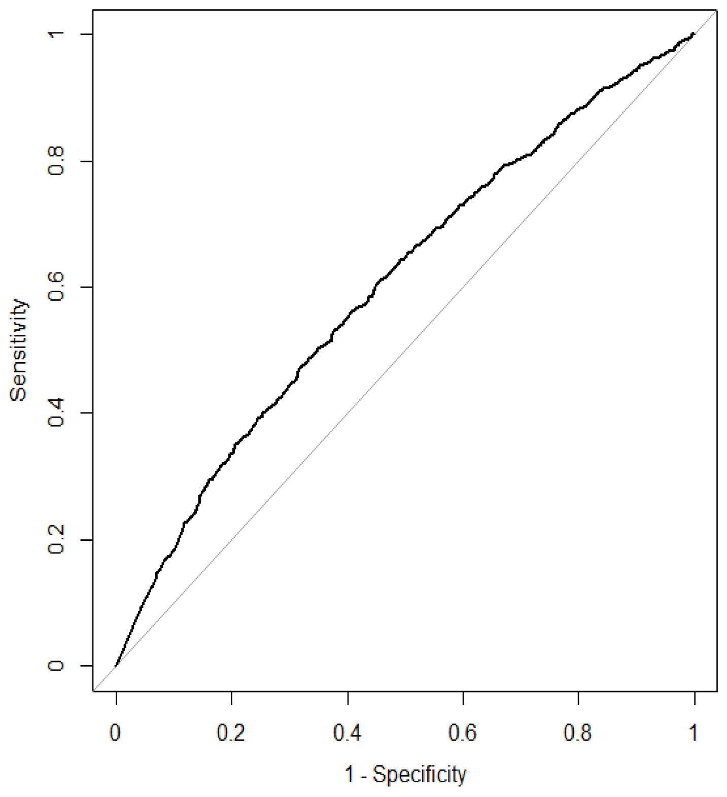
Figure 1.
Receiver operating characteristic (ROC) curve for bagging. (Area under the curve (AUC) = 0.575, F-score = 0.520).
Figure 1.
Receiver operating characteristic (ROC) curve for bagging. (Area under the curve (AUC) = 0.575, F-score = 0.520).

Figure 2.
ROC curve for boosting. (AUC = 0.769, F-score = 0.744).

Figure 3.
ROC curve for random forest. (AUC = 0.605, F-score = 0.714).

Figure 4.
ROC curve for deep neural network (DNN) (Tanh). (AUC = 0.753, F-score = 0.721).

Figure 5.
ROC curve for neural network (NN) (Tanh). (AUC = 0.768, F-score = 0.741).

Figure 6.
ROC curve for DNN (Tanh w/Dropout). (AUC = 0.600, F-score = 0.620).

Figure 7.
ROC curve for NN (Tanh w/Dropout). (AUC = 0.704, F-score = 0.717).

Figure 8.
ROC curve for DNN (ReLU). (AUC = 0.751, F-score = 0.734).

Figure 9.
ROC curve for NN (ReLU). (AUC = 0.757, F-score = 0.727).

Figure 10.
ROC curve for DNN (ReLU w/Dropout). (AUC = 0.765, F-score = 0.735).

Figure 11.
ROC curve for NN (ReLU w/Dropout). (AUC = 0.767, F-score = 0.730).

Table 1.
Confusion matrix.
| Actual Class | |||
|---|---|---|---|
| Event | No-Event | ||
| Predicted Class | Event | TP (True Positive) | FP (False Positive) |
| No-Event | FN (False Negative) | TN (True Negative) | |
Table 2.
Prediction accuracy of each method for original data.
| (a) Original data: the ratio of training and test data is 75% to 25% | ||||||
| Method | Accuracy Ratio of Training Data | Accuracy Ratio of Test Data | ||||
| Average (%) | Standard Deviation | Average (%) | Standard Deviation | |||
| Bagging | 80.13 | 0.003 | 55.98 | 0.008 | ||
| Boosting | 71.66 | 0.003 | 71.06 | 0.008 | ||
| Random Forest | 69.59 | 0.544 | 58.50 | 0.844 | ||
| Method | Accuracy Ratio of Training Data | Accuracy Ratio of Test Data | ||||
| Model | Activation Function | Middle Layer | Average (%) | Standard Deviation | Average (%) | Standard Deviation |
| DNN | Tanh | 2 | 70.66 | 0.721 | 68.93 | 0.972 |
| NN | Tanh | 1 | 71.01 | 0.569 | 69.59 | 0.778 |
| DNN | Tanh with Dropout | 2 | 58.47 | 3.566 | 58.46 | 3.404 |
| NN | Tanh with Dropout | 1 | 67.27 | 1.237 | 67.14 | 1.341 |
| DNN | ReLU | 2 | 69.57 | 0.707 | 68.61 | 0.863 |
| NN | ReLU | 1 | 68.81 | 0.708 | 68.30 | 1.008 |
| DNN | ReLU with Dropout | 2 | 69.97 | 0.903 | 69.01 | 0.956 |
| NN | ReLU with Dropout | 1 | 70.12 | 0.637 | 69.48 | 0.881 |
| (b) Original Data: the Ratio of Training and Test Data is 90% to 10% | ||||||
| Method | Accuracy Ratio of Training Data | Accuracy Ratio of Test Data | ||||
| Average (%) | Standard Deviation | Average (%) | Standard Deviation | |||
| Bagging | 79.58 | 0.003 | 56.23 | 0.015 | ||
| Boosting | 71.57 | 0.003 | 70.88 | 0.011 | ||
| Random Forest | 68.55 | 0.453 | 58.77 | 1.331 | ||
| Method | Accuracy Ratio of Training Data | Accuracy Ratio of Test Data | ||||
| Model | Activation Function | Middle Layer | Average (%) | Standard Deviation | Average (%) | Standard Deviation |
| DNN | Tanh | 2 | 69.64 | 0.683 | 69.31 | 1.325 |
| NN | Tanh | 1 | 70.49 | 0.550 | 69.61 | 1.312 |
| DNN | Tanh with Dropout | 2 | 57.29 | 3.681 | 57.27 | 4.117 |
| NN | Tanh with Dropout | 1 | 66.37 | 1.619 | 66.25 | 1.951 |
| DNN | ReLU | 2 | 69.49 | 0.695 | 68.76 | 1.408 |
| NN | ReLU | 1 | 69.16 | 0.728 | 68.54 | 1.261 |
| DNN | ReLU with Dropout | 2 | 69.74 | 0.796 | 68.84 | 1.438 |
| NN | ReLU with Dropout | 1 | 70.26 | 0.573 | 69.55 | 1.210 |
Table 3.
Prediction accuracy of each method for normalized data.
| (a) Normalized data: the ratio of training and test data is 75% to 25% | ||||||
| Method | Accuracy Ratio of Training Data | Accuracy Ratio of Test Data | ||||
| Average (%) | Standard Deviation | Average (%) | Standard Deviation | |||
| Bagging | 80.12 | 0.003 | 56.15 | 0.008 | ||
| Boosting | 71.66 | 0.004 | 70.95 | 0.007 | ||
| Random Forest | 69.67 | 0.565 | 58.39 | 0.880 | ||
| Method | Accuracy Ratio of Training Data | Accuracy Ratio of Test Data | ||||
| Model | Activation Function | Middle Layer | Average (%) | Standard Deviation | Average (%) | Standard Deviation |
| DNN | Tanh | 2 | 71.14 | 0.732 | 68.75 | 0.912 |
| NN | Tanh | 1 | 70.64 | 0.652 | 69.42 | 0.763 |
| DNN | Tanh with Dropout | 2 | 57.00 | 4.324 | 56.69 | 4.485 |
| NN | Tanh with Dropout | 1 | 68.09 | 0.641 | 68.01 | 0.904 |
| DNN | ReLU | 2 | 70.37 | 0.627 | 69.35 | 0.856 |
| NN | ReLU | 1 | 70.92 | 0.615 | 69.37 | 0.943 |
| DNN | ReLU with Dropout | 2 | 70.00 | 0.811 | 68.96 | 0.946 |
| NN | ReLU with Dropout | 1 | 70.25 | 0.692 | 69.56 | 0.813 |
| (b) Normalized data: the ratio of training and test data is 90% to 10% | ||||||
| Method | Accuracy Ratio of Training Data | Accuracy Ratio of Test Data | ||||
| Average (%) | Standard Deviation | Average (%) | Standard Deviation | |||
| Bagging | 79.54 | 0.003 | 56.28 | 0.013 | ||
| Boosting | 71.50 | 0.003 | 70.80 | 0.012 | ||
| Random Forest | 68.66 | 0.475 | 58.83 | 1.368 | ||
| Method | Accuracy Ratio of Training Data | Accuracy Ratio of Test Data | ||||
| Model | Activation Function | Middle Layer | Average (%) | Standard Deviation | Average (%) | Standard Deviation |
| DNN | Tanh | 2 | 70.18 | 0.698 | 69.35 | 1.382 |
| NN | Tanh | 1 | 70.52 | 0.594 | 69.51 | 1.309 |
| DNN | Tanh with Dropout | 2 | 58.04 | 5.134 | 58.14 | 5.016 |
| NN | Tanh with Dropout | 1 | 67.33 | 1.285 | 67.13 | 1.787 |
| DNN | ReLU | 2 | 71.41 | 0.710 | 69.17 | 1.334 |
| NN | ReLU | 1 | 69.55 | 0.772 | 68.97 | 1.426 |
| DNN | ReLU with Dropout | 2 | 69.76 | 0.785 | 69.13 | 1.426 |
| NN | ReLU with Dropout | 1 | 69.88 | 0.701 | 69.25 | 1.279 |
© 2018 by the authors. Licensee MDPI, Basel, Switzerland. This article is an open access article distributed under the terms and conditions of the Creative Commons Attribution (CC BY) license (http://creativecommons.org/licenses/by/4.0/).
Share and Cite
MDPI and ACS Style
Hamori, S.; Kawai, M.; Kume, T.; Murakami, Y.; Watanabe, C. Ensemble Learning or Deep Learning? Application to Default Risk Analysis. J. Risk Financial Manag. 2018, 11, 12. https://0-doi-org.brum.beds.ac.uk/10.3390/jrfm11010012
AMA Style
Hamori S, Kawai M, Kume T, Murakami Y, Watanabe C. Ensemble Learning or Deep Learning? Application to Default Risk Analysis. Journal of Risk and Financial Management. 2018; 11(1):12. https://0-doi-org.brum.beds.ac.uk/10.3390/jrfm11010012
Chicago/Turabian StyleHamori, Shigeyuki, Minami Kawai, Takahiro Kume, Yuji Murakami, and Chikara Watanabe. 2018. "Ensemble Learning or Deep Learning? Application to Default Risk Analysis" Journal of Risk and Financial Management 11, no. 1: 12. https://0-doi-org.brum.beds.ac.uk/10.3390/jrfm11010012