Defining Data Science by a Data-Driven Quantification of the Community


1
Predictive Medicine and Data Analytics Lab, Department of Signal Processing, Tampere University of Technology, FI-33101 Tampere, Finland
2
Institute of Biosciences and Medical Technology, FI-33101 Tampere, Finland
3
Institute for Intelligent Production, Faculty for Management, University of Applied Sciences Upper Austria, Steyr Campus, A-4400 Steyr, Austria
4
Department of Mechatronics and Biomedical Computer Science, UMIT, A-6060 Hall in Tyrol, Austria
5
College of Computer and Control Engineering, Nankai University, Tianjin 300071, China
*
Author to whom correspondence should be addressed.
Mach. Learn. Knowl. Extr. 2019, 1(1), 235-251; https://0-doi-org.brum.beds.ac.uk/10.3390/make1010015
Submission received: 4 December 2018
/
Revised: 14 December 2018
/
Accepted: 17 December 2018
/
Published: 19 December 2018
(This article belongs to the Section Data)
Abstract
:Data science is a new academic field that has received much attention in recent years. One reason for this is that our increasingly digitalized society generates more and more data in all areas of our lives and science and we are desperately seeking for solutions to deal with this problem. In this paper, we investigate the academic roots of data science. We are using data of scientists and their citations from Google Scholar, who have an interest in data science, to perform a quantitative analysis of the data science community. Furthermore, for decomposing the data science community into its major defining factors corresponding to the most important research fields, we introduce a statistical regression model that is fully automatic and robust with respect to a subsampling of the data. This statistical model allows us to define the ‘importance’ of a field as its predictive abilities. Overall, our method provides an objective answer to the question ‘What is data science?’.
1. Introduction
From time to time new scientific fields emerge as a consequence to adapt to a changing world. Examples for the establishment of new academic disciplines are economy (the first professorship in economics was established at the University of Cambridge in 1890 held by Alfred Marshall [1]), computer science (the first department of computer science in the United States was established at Purdue University in 1962 whereas the term ‘computer science’ has appeared first in [2]), bioinformatics (the term was first used by [3]) and most recently data science [4,5,6]. The first appearance of the term ‘data science’ is ascribed to Peter Naur in 1974 [7] but it took nearly 30 years until there were callings for an independent discipline with this name [8]. Since then, the first Research Center for Dataology and Data Science was established at Fudan University in Shanghai, China, in 2007 and Harvard Business Review called “Data Scientist: The Sexiest Job of the 21st Century” [9].
A question asked by many is ‘What is data science?’ and there are many contributions attempting to provide adequate definitions or characterizations of the field [10,11,12,13,14,15]. A commonality all of these papers is that they present a qualitative, descriptive list of attributes in an argumentative way.
In contrast, in this paper we present a data-driven, quantitative approach. Interestingly, that means we are using methods from data science in order to define data science itself. The data we are using for our analysis are from Google Scholar. According to a study by [16] the number of scholarly documents indexed by Google Scholar has been estimated to be 160–165 million. Furthermore, it has been estimated that Google Scholar covers about 87% of all scholarly publications [17]. This makes Google Scholar an authoritative academic search engine. Importantly, in addition to this information, Google Scholar allows scientists to create a summary page where scientists can enter a list of research interests. This means Google Scholar provides not only publication statistics but also curated research interests of scientists. Taken together, this makes it a unique source of information to study scholarly activity.
By using data from Google Scholar from scientists who declare a research interest in ‘data science’, we study various publication statistics providing information about the scientists and the research fields they are interested in. Furthermore, for decomposing the data science community into its major defining fields or core fields, we introduce two quantitative methods. The first method is a deterministic method, whereas the second method is a statistical model. Despite the different nature of the two methods, we demonstrate that both methods are robust for a subsampling of the data.
We presented two methods instead of one for better highlighting the significance of Method-2 (see Section 3.6.2). Specifically, Method-1 (see Section 3.6.1) is semi-automatic requiring the manual specification of a threshold. In contrast, Method-2 is an automatic method using the Bayesian information criterion (BIC) [18] to estimate such a threshold. Another difference between the methods is the definition of ‘importance’ to identify the core fields of the data science community. For Method-1, we use the norm of a vector, whereas for Method-2 we use the LMG method [19] allowing to determine the contribution of a predictor to for a regression model. It is the statistical nature of Method-2 that allows the definition of ‘importance’ from a statistical perspective. For all of these reasons, we consider Method-2 as the favorable approach and its results as the main spanning factors of the data science community, hence, providing an objective answer to the question ‘What is data science?’.
In our opinion, our scientometrics study [20,21] of data science is the first of its kind. By providing a fully automatic, comprehensive account for identifying the major influences of data science based on a quantitative analysis of curated scholarly data we contribute to an objective definition of this field. Beyond our study, our approach could be applied to other emerging fields to quantify these in a similar way.
Our paper is organized as follows. In the next section, we present the data and methods we are using for our analysis. In the results section we present our findings, then the following section provides a discussion and implications. This paper ends with concluding remarks.
2. Methods
In this section, we describe first the data we are using for our analysis. Then we describe a enrichment analysis and an importance analysis of a regression model we apply to the data.
2.1. Data
Our analysis is based on data from Google Scholar (https://0-scholar-google-com.brum.beds.ac.uk/). Google Scholar started in 2004 as a freely accessible repository providing information of scholarly literature, scientists and fields across many disciplines. It indexes automatically most peer-reviewed online academic journals, books and conference articles and other scholarly literature. In addition, it allows scientists to create a summary page of their academic publications and enter scientific fields they are interested in.
We implemented an R script that allows to download information of all scientists that indicated an interest in ‘data science’. Overall, as of March 2018, we find 4460 scientists that declare such an interest. For each of these scientists we obtain information about
- total number of citations
- research interests
- affiliation
which we use for our analysis.
2.2. Enrichment Analysis
For finding enriched scientific fields with highly cited scientists, we apply an enrichment analysis [22]. Our procedure works the following way. First, we are rank ordering all scientists according to their number of citations. Second, we group this list of scientists into two subcategories by introducing a threshold . If the number of citations is above this threshold, we place this scientist in category ‘HC-Yes’, otherwise in category ‘HC-No’. That means we are distinguishing between scientists that have been highly cited or not. Third, we give each scientist a second attribute, ‘Field’. If a scientist has an interest in a specific ‘Field’ we give the scientist the label ‘Field-In’, otherwise ‘Field-Out’. That means we are distinguishing between scientists that have an interest in a specific field or not. As a result, each scientist has now two attributes on which we base our enrichment analysis.
In Table 1 we give a formal overview of this resulting in a contingency table. Each element in the table corresponds to a count value obtained in the way described above. Here
gives the total number of scientists interested in a particular field and
gives the number of scientists not interested in this field. Similarly,
gives the total number of highly cited scientists and
give the total number of scientists not highly cited. Furthermore, gives the total number of scientists studied.
The Null Hypothesis we are studying for each field Y can be formulated by the following statement:
Hypothesis 1 (Null hypothesis: H0).
The probability for a scientist to be declared highly cited (‘HC-yes’) and interested in field Y ‘Field-In’ is the same as the probability for a scientist to be declared highly cited (‘HC-yes’) and not interested in field Y ‘Field-Out’?
The exact sampling distribution for this null hypothesis H0 is given by [23]
From the sampling distribution, we estimate the p-value by
For assessing the statistical significance we use a significance level of with a Bonferroni correction.
2.3. Importance of Fields
For quantifying the importance of fields we use a regression analysis and a method for quantifying the relative importance of predictors (in our analysis fields correspond to predictors). We do this by determining the contribution of a predictor to for a regression model. However, it has been realized that with correlated predictors such an decomposition approach is difficult due to the fact that the ordering of the predictors gives a different decomposition of the sum of squares of the model. For this reason, Lindeman, Merenda, and Gold [19] proposed a procedure, called LMG, to average over all orderings of predictors [24].
LMG is based on a sequential decomposition of s (coefficient of determination),
For n regressors, , let the vector indicate the permutations of the n indices and let denote the set of predictors ordered according to r, before the new predictor is added to the model. For this situation, Equation (7) can be written as [25]
From this one obtaines LMG by
Due to of the averaging over permutations, this is computationally demanding. Evaluating Equation (9) for all predictors gives the importance for these. One can show that LMG decomposes into non-negative contributions that sum to the total [25]. Hence, by normalizing LMG by the total one obtains the percentage of this decomposition.
2.4. Numerical Analysis
For our numerical analysis we use the statistical programming language R [26].
3. Results
3.1. Scientific Fields
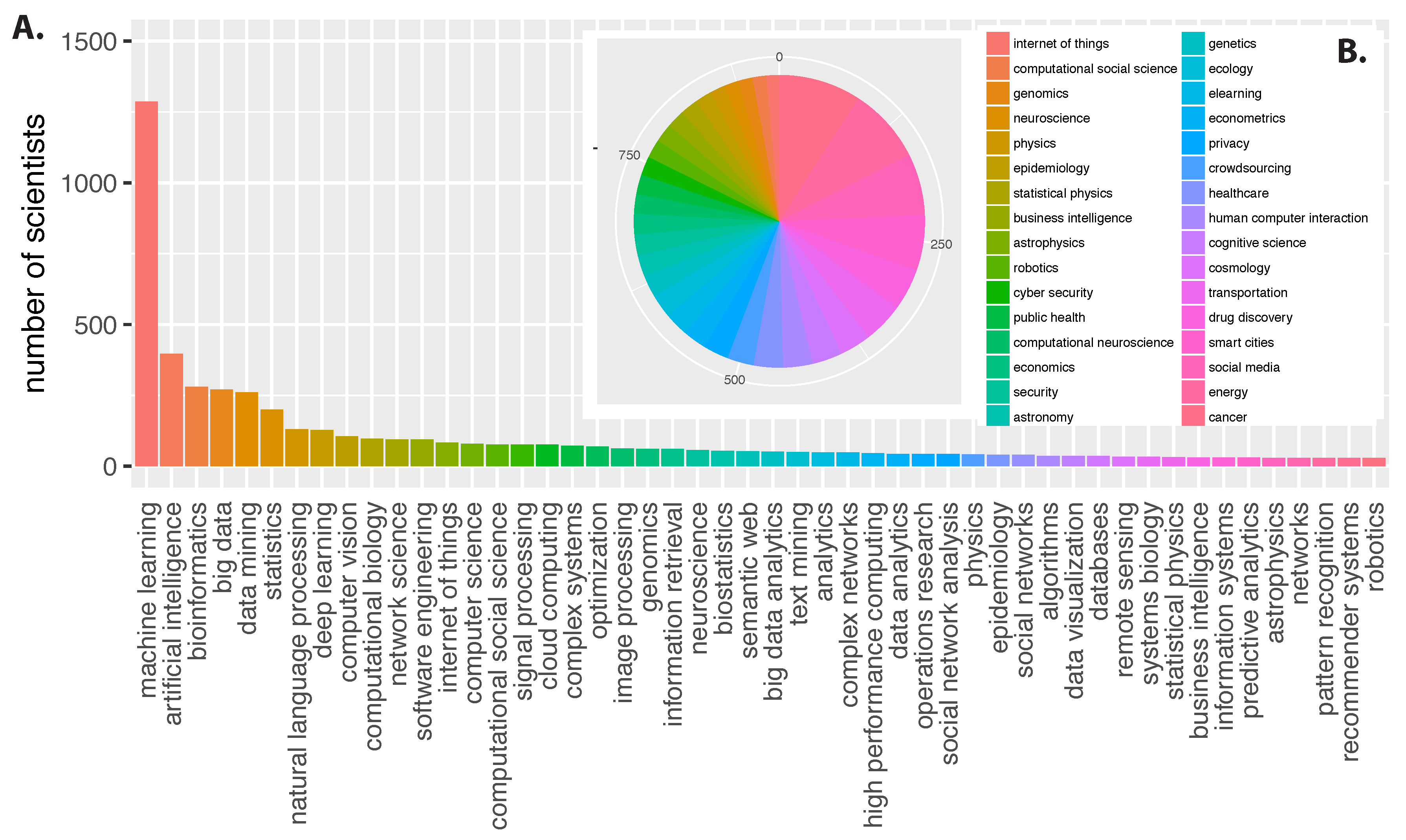
We start our analysis by showing the frequency counts for the top 50 fields, see Figure 1A. That means for each scientific field, we count how many scientists named this field among their research interests. As one can see, ‘machine learning’ is the by far most frequent field followed by ‘artificial intelligence’ and ‘bioinformatics’. After the sixth field (‘statistics’) all other counts are rapidly decaying. From our data we find in total 4040 unique research fields used by the community to describe their research interests. Given the fact that the total number of scientists in our data is 4460 this indicates a very wide interest range of the community.
In Figure 1B we show the top 32 non-technical fields of the data science community with a focus on applications. That means these fields are not computer science or machine learning related but have a clear focus on the application domain. For these fields the minimal frequency is 13 (‘cancer’) and the maximal frequency is 84 (‘internet of things’) followed by ‘computational social science’ with 77 and ‘genomics’ with 62. The pie chart shows the corresponding frequencies.
3.2. Global Community Landscape
In order to obtain a global overview among the connection between the different fields we infer a global network representation. Specifically, we are using the top 50 fields from Figure 1A as variables and apply the BC3Net network inference method [27]. Each field is represented by a binary vector of length , corresponding to the number of scientists, where a ‘1’ indicates a research interest of a scientist in the field and a ‘0’ the lack of such an interest.
The basic idea of BC3Net is a bagging version of C3Net [28] which gives conservative estimates of the relations between the variables using estimates of mutual information values. Previously, this method has been successfully used in genomics to infer causal gene regulatory networks from high-dimensional data [29,30] and in finance for inferring investor trading networks [31].
To obtain a robust network we generate 1000 Bootstrapping data sets on which the BC3Net will be based. These Bootstrapping data sets are generated by sampling with replacement of the components of the profile vectors, corresponding to the scientists.
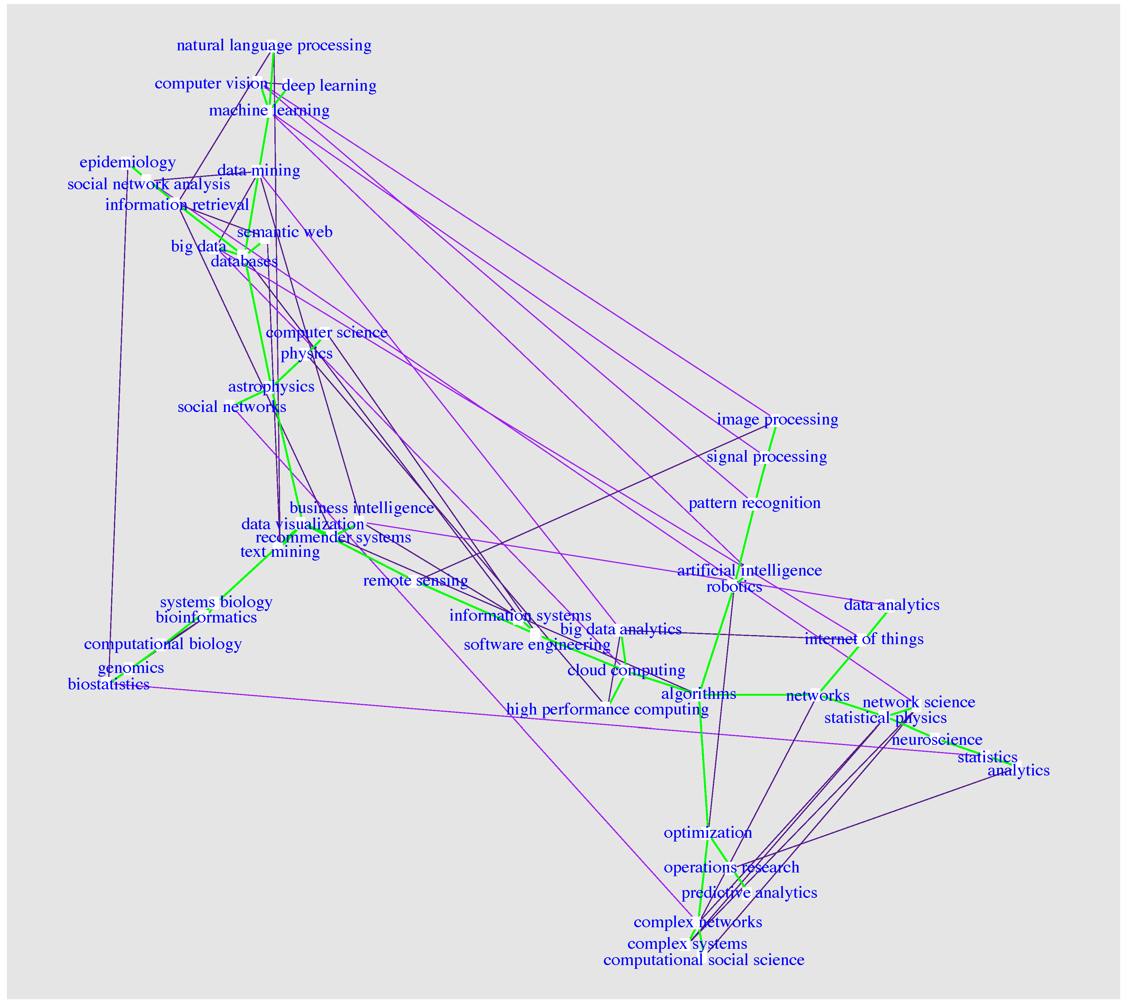
The resulting network is shown in Figure 2. This network contains 88 edges between the 50 fields and, hence, is a sparse network with an edge density of 0.072. The network is connected and the minimum spanning tree (MST) [32] of the network is shown by the green edges in Figure 2. MST means that the edges in this tree are sufficient in order to obtain a connected network. Hence, these connections are not redundant. For this reason the MST can be seen as the backbone of the network that connects everything (every field) with each other.
There are several clusters visible in the network reflecting domain specific sub-communities. For instance, the fields biostatistics, genomics, computational biology, bioinformatics and systems biology are closely connected. Similarly, image processing, signal processing and pattern recognition or high performance computing, cloud computing, software engineering, big data analytics and informations systems. The intuitive similarity of these fields indicates that the shown network in Figure 2 has a meaningful structure that summarizes the complex relationships between the fields.
3.3. Scientists in the Community
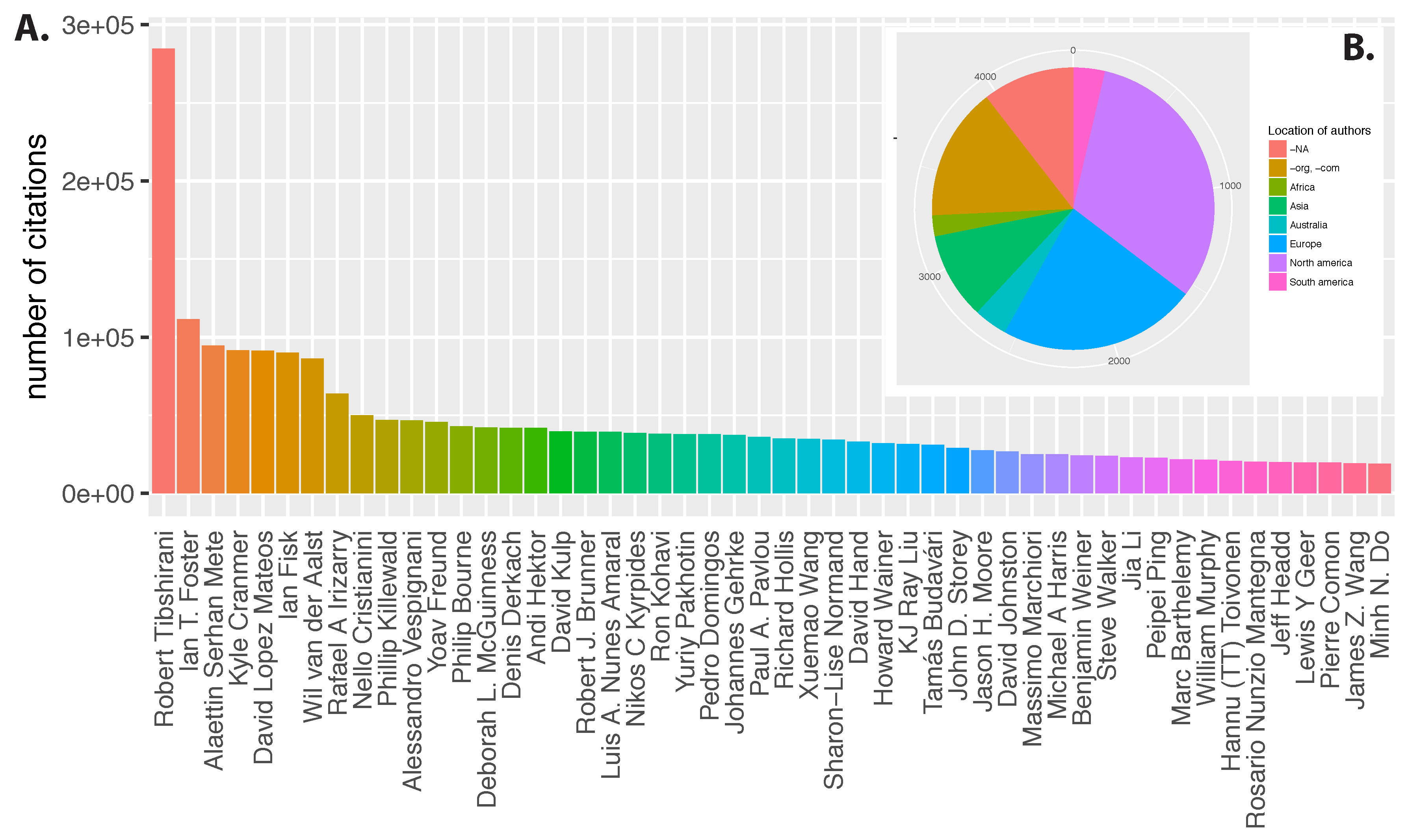
Next, we study the scientists in the community. In Figure 3A we show the top 50 scientists ranked according to their number of citations in the data science community. Similar to the frequency counts of the fields (shown in Figure 1A) also for the number of citations we find only one author (Robert Tibshirani) that has significantly more publications than everyone else with a rapid decay after the seventh author (Wil van der Aalst). The community size of the whole community (number of scientists) is 4460.
To learn about the location of the scientists we used information from the provided email registration. From these we extracted the email extension to identify the location of the scientists. In Figure 3B we show a summary of the results. We could identify 1399 scientists from North America and 1003 from Europe. From these, 233 scientists come from the UK and 119 from Germany. These two countries are the largest communities in Europe. Overall, North America and Europe are clearly dominating the community. It is interesting to note that despite the dominance of these two regions, there are scientists from all continents in the community. Figure 3B includes also information about emails ending in ‘org’ or ‘com’ (672 scientists) and 463 scientists with an unregistered or unrecognizable email, indicated by ‘NA’. The proportion of such scientists for whom no definite location information can be obtained (comprising ‘org’, ‘com’ and ‘NA’) is 25.4%.
3.4. Enrichment of Fields
The next analysis we perform is an enrichment analysis. In this analysis, we study whether the scientists with the highest number of citations in data science prefer to work in particular fields.
To perform such an enrichment analysis we need to assign to the scientists two attributes. The first attribute indicates if a scientist is highly cited or not, and the second attribute indicated if a scientist is interested in a particular field or not. We assign these attributes in the following way. First, we are rank ordering all scientists according to their number of citations. Second, we group this list of scientists into two subcategories by introducing a threshold. If the number of citations is above this threshold, we place this scientist in category ‘HC-Yes’, otherwise in category ‘HC-No’. That means we are distinguishing between scientists that have been highly cited (HC) or not. Third, we give each scientist a second attribute, ‘Field’. If a scientist has an interest in a specific ‘Field’ we give the scientist the label ‘Field-In’, otherwise ‘Field-Out’. That means we are distinguishing between scientists that have an interest in a particular field or not. As a result, each scientist has now two attributes on which we base our enrichment analysis (see Methods Section 2 for details).
In our procedure, we have one parameter, namely the threshold to distinguish between highly cited scientists and the rest. This parameter is just the number of scientists we consider as highly cited. In Table 2 we show the results of our enrichment analysis with Bonferroni correction for the 52 fields with the highest number of total citations. The number in the first row, correspond to this number of highly cited scientists (called top scientists). The largest threshold we are using is 2000 which corresponds to almost 50% of all scientists and, hence, is very anti-conservative. As we see, by increasing the number of scientists we consider highly cited (moving to the right hand-side of the table) the number of significant fields increases. On the other hand, for a threshold of 10, only the field ‘robotics’ tests significantly.
Overall, we are making the following observations. First, regardless of the chosen threshold, there are always some fields significant. This means there are indeed differences in research interests of scientists highly cited. Second, selecting one particular threshold to define highly cited scientists is subjective. However, it is clear that whatever value it should be this can only include a few percentage of all scientists. For this reason, 100 corresponding to 2.5% (=100/4060) of all scientists, is one sensible possible choice. For this threshold, we find ‘statistics’ and ‘robotics’ to be significant. Third, starting with 52 fields of our analysis, we find only a very few fields significant. Even for a threshold of 2000 there are only 8 fields enriched.
3.5. Joint Properties and Composition of the Community
Next, instead of studying individual properties of the community as in the last sections, we study now joint properties of the data science community. To do this, we analyze scientists and research fields together. In the following we call the research interests briefly ‘fields’.
First, put simply, we are interested in characterizing how many scientists are covered by how many fields. To do this we are rank ordering the fields according to number of scientists interested in and count the number of scientists that are interested in any of these fields. By successively removing fields and repeating the counting of the scientists we obtain the number of scientists in dependence on the rank ordering of the fields. This means every point on the resulting curve corresponds to (I) a group of fields and (II) a group of scientists. Both groups can be characterized. For instance, for each field in the group of fields one can determine the number of scientists interested in, allowing to identify the field with the minimal number of scientists. Hence, a group of fields can be characterized by the minimal number of scientists interested in any of these fields.
In the following, we consider D the binary data matrix whereas the number of rows corresponds to the number of scientists and the number of columns to the number of fields . If it means that scientist i has a research interest in field j. For instance, to identify how many fields are named by 10 or more scientists we are calculating
Here is the theta function that gives one if its argument is true, and otherwise zero. From this, we find 157 fields with this property.
From D we obtain a vector of length where its component corresponds to the number of scientists interested in field j by
We use this vector to obtain a ranking of the fields in declining order according to their sizes
Here the components of the vector correspond to the indices of the fields in a way that give the size of the fields in declining order, i.e., .
We are using the ordering of the sizes of the fields by successively removing fields from D to calculate how many scientists are covered by the remaining fields. Formally, this can be done by
Here we define as the set that includes all elements of up to index and as the empty set. Furthermore, ‘’ is the set difference operator that eliminates all elements in X from Y. That means goes only over the fields that rank higher than k. For instance, using Equation (13) we obtain for and for .
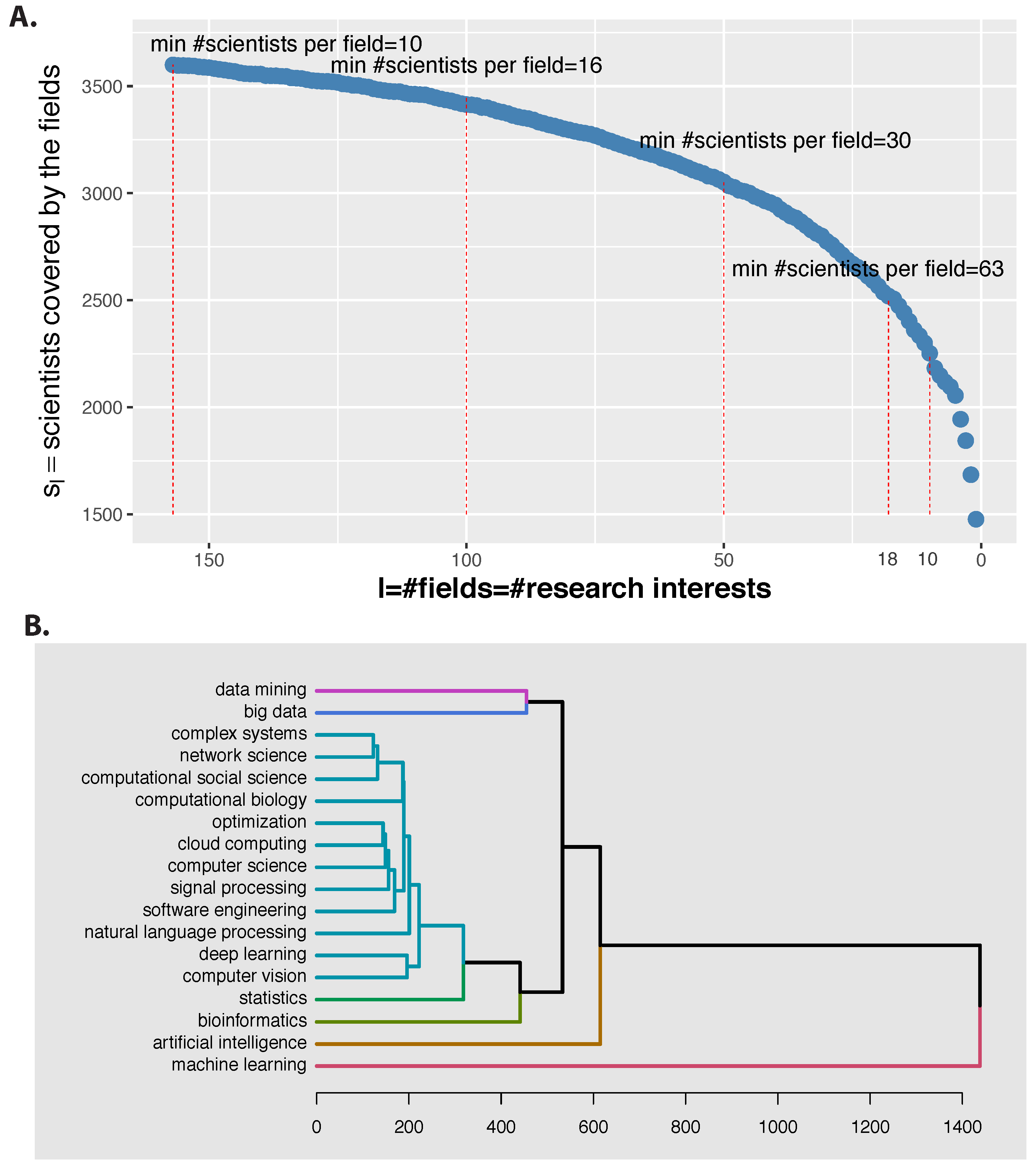
In Figure 4A, we show the results. We limit in this figure our focus to (or less fields), which corresponds to removing fields. This leaves us with scientists that have together only l different research interests. From Figure 4A one can see that the number of scientists covered by a certain number of fields (x-axis) is monotonously decreasing until the minimal number of is reached for the last field (‘machine learning’). Interestingly, the values of gives the minimal number of scientists for all of these l fields, which is for the leftmost point in Figure 4A. For further selected values of l we give the corresponding values in the figure.
From Figure 4A, we can make two major observations that are important for the next section. First, despite the fact that in total we have 4040 research interests (fields), which is a very large number, only 157 fields attract 10 or more scientists. If one considers the fields as variables and the scientists as samples then it is clear that for any statistical model that builds on these variables and samples, a sufficient size of samples is required for obtaining robust results. Statistical models using variables with less than 10 samples are unlikely to result in robust estimates. For this reason, Figure 4A is informative for assessing the potential quality and the number of fields as characterized by the minimal number of scientists (samples). In the next section, we will introduce a statistical model (Method-2) that will automatically perform a feature selection, but Figure 4A allows to understand the size of the resulting feature set.
The second major observation from Figure 4A is that the number of scientists covered by a few fields is still in the thousands. For instance, for we have scientists and for we find even scientists. That means even when we are reducing the number of fields considerably in a way as described above, we are still covering a large proportion of all scientists of the community.
Based on the above findings, we want to obtain a conservative overview about the connections among the largest fields in the community. For this reason, we select the 18 largest fields (having a minimal number of 63 scientists per field (see Figure 4A)) and perform a hierarchical clustering for these fields. In Figure 4B, we show the result using a Manhattan distance and a complete linkage clustering. Interestingly, the field ‘machine learning’ has the farthest distance to all other fields indicating that scientists with this interest work on many more fields beyond the 17 used in our analysis. This makes ‘machine learning’ the most diverse field of all. The second most diverse field is ‘artificial intelligence’. All other fields are more similar to each other with the mild exception of ‘data mining’ and ‘big data’.
3.6. Decomposition of the Community
After obtaining an overview of the community by studying its composition in the last sections, we present in the following two methods for decomposing the community. By ‘decomposing’ we mean the identification of major fields that span the data science community. The first method (Method-1) we introduce is semi-automatic with an intuitive interpretation whereas the second method (Method-2) is fully automatic and statistically well defined.
3.6.1. Method-1
Our first method for decomposing the community is based on the realization that we are having two different pieces of information available that make contributions to the community. The first one is about the number of citations and the second one is about the number of scientists interested in a particular field. Based on these two components we define a measure below, we are using for ranking the importance of the fields.
Specifically, for the quantification of ‘contribution to the community’ we are using the two variables, (I) the number of citations in a field i, , and (II) the number of scientists in a field i, . The number of scientists corresponds to the number of researcher using a particular label to express their research interest in a field, e.g., ‘statistics’ or ‘natural language processing’, whereas the number of citations corresponds to the total number of citations contributed by all scientists interested in a particular field. To make these numbers comparable, we normalize both by the maximal number of observed citations and scientists respectively. This results in the characterization of each field i by the two-dimensional vector,
For these vectors we quantify the contribution of each field by the Euclidean norm of their corresponding vectors. Finally, we normalize these contributions to obtain the percentage of these contributions.
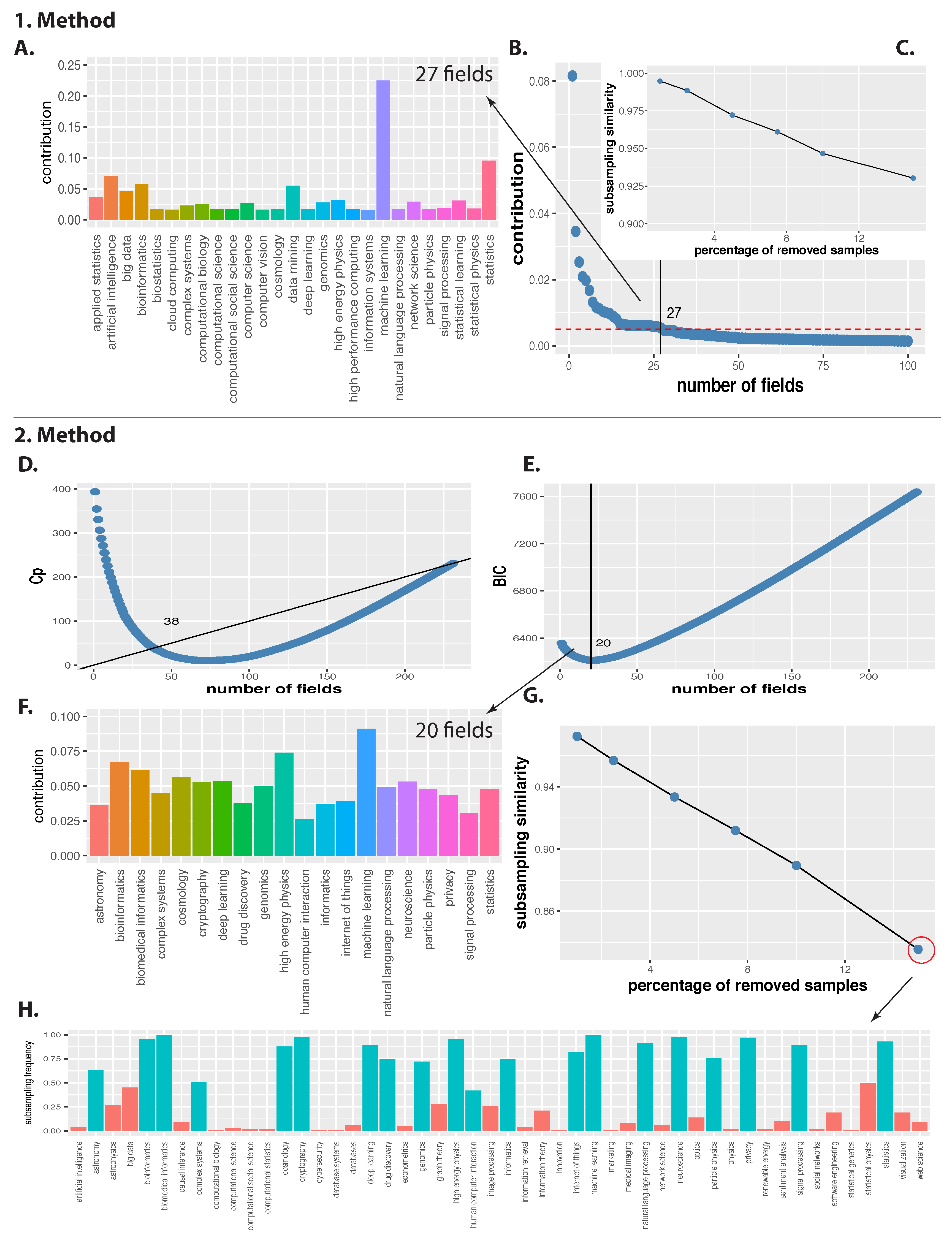
In Figure 5B, we show the ranking of these contributions. We show only the first 100 fields because the contribution values are rapidly decreasing, as one can see. It is interesting to note that only very few fields have much larger contributions than all others. Specifically, the top 12 fields contribute together almost 25% (from a cumulative distribution, not shown).
In Figure 5B, we added a dashed red line indicating a contribution of 0.005, which corresponds to 27 fields. The reason for choosing this threshold is motivated by the dip in the curve in Figure 5B and our results shown in Figure 4A. The detailed contributions of these 27 fields are shown in In Figure 5A. Overall, ‘machine learning’ makes by far the largest contribution followed by ‘statistics’.
To study the robustness of our results, we subsample the data. Specifically, we subsample the data by removing a certain percentage of samples and repeat the analysis. Here a sample corresponds to research interests of a scientist, hence, we repeat the analysis for randomly selecting a certain percentage of scientists which we exclude from our analysis. This mimics to some extend the randomness with which scientists register in Google Scholar. As a result we see if the top fields change or remain robust for the smaller data sets.
We measure the similarity of the randomized and nonrandomized analysis by quantifying the overlap of the fields in common as
Here is the optimal number of fields we estimated from the whole data set, corresponds to the number of subsampled data sets and ‘prs’ means ‘percentage of removed samples’.
The results from this analysis are shown in Figure 5C. Overall, removing up to 15% of the samples (corresponding to the scientists) results in over 90% similarity in the fields. This indicates that our results are highly robust.
3.6.2. Method-2
The second decomposition we are defining, is based on the predictive abilities of the fields. For this, we are applying a two-step procedure. In the first step, we identify the key fields with respect to their predictive abilities. In the second step we quantify these by estimating their importance for the predictions.
For step one, we perform a forward-stepwise regression (FSR) [33]. The FSR starts with the simplest model and enters successively one regressor (field) at a time. This builds a sequence of models. Specifically, at each stage of this stepwise procedure we enter the repressor that is most correlated with the residuals. This process is repeated until either all predictors have been entered, or the residuals are zero.
Our regression model is defined by
where the s are the regression coefficients, the are the predictors and represents the unexplained part. For the index i corresponds to a scientist and j to a field. The predictors can only assume two values because either scientist i has an interest in research field j, corresponding to , or not, indicated by . The value of gives the natural logarithm of the total number of citations of scientist i. We used a logarithmic scaling because the number of citations of the scientists varies considerably (see Figure 3) and the logarithmic scaling prevents that individual scientists with a very large number of citations dominate the model.
The result of this step are summarized in Figure 5D,E. Specifically, we are showing two goodness-of-fit measures, Mallow’s Cp [34,35] and the BIC (Bayesian information criterion) [18]. Regarding their interpretation, it is suggested to choose the Cp statistic approaching p (the number of repressors) from above. For the BIC, which is a variant of the AIC (Akaike information criterion)—with a stronger penalty for including additional variables to the model, the model with the lowest BIC should be selected. In Figure 5D,E the optimal values of Cp and BIC are indicated by the intersections with the black lines.
As one can see from Figure 5D,E, the statistical estimates for the number of fields that should be included in the model vary between 20 (for BIC) and 38 (for Cp). Beyond these numbers, the Cp- and BIC-curve clearly indicate that adding further fields (parameters) to the regression model leads only to marginal effects. It is known that Cp provides more relaxed estimates than BIC including all parameters of relevance to the model, whereas BIC is more conservative focusing on the major core of parameters. That means Mallow’s Cp is more likely to include false positives than BIC but less likely to have false negatives. Here we are interested in the major fields forming the core of data science community and for this reason we are using BIC as our selection criterion.
Based on the BIC results, we select the 20 fields with the highest contribution. For these fields we perform an additional regression, limited to those fields only. Then for the resulting model, we estimate the relative importance of the fields by using the method LMG [19] for determining the contribution of a predictor to for the regression model (see the Methods Section 2.3 for details).
In Figure 5F, we show the result of this importance analysis for the 20 fields. Overall, the top four fields are: machine learning, high energy physics, bioinformatics and biomedical informatics, whereas machine learning is clearly the most important field. Beyond these four fields, all others are similar in their importance except human-computer-interaction and signal processing, which are lowest.
To study the robustness of these results, we preform a subsampling analysis (see Method-1). We quantify the outcome with the subsampling similarity (subsim) as
Here is the optimal number of fields we estimated from the whole data set using BIC, corresponds to the number of subsampled data sets and ‘prs’ means ‘percentage of removed samples’.
In Figure 5G we show results for prs {1%, 2.5%, 5%, 7.5%, 10%, 15%}. For removing up to 5% of the samples, we observe a very high similarity of over 93% and even for removing 15% of all samples, we still have a similarity of almost 85%. This indicates a high robustness of the identified fields.
Finally, in Figure 5H, we show the subsampling frequency of individual fields for 15% removed samples. In contrast to the subsampling similarity, we defined for estimating the similarity with the whole set of the 20 optimal fields, the subsampling frequency gives the appearance frequency of individual fields in the subsampled data. The green bars indicate the 20 major fields identified by BIC, whereas the red bars correspond to further fields beyond this set of fields that appeared during the subsampling. As one can clearly see, the subsampling frequency for the 20 major fields is always higher than for these additional fields except for ‘human computer interaction’.
4. Discussion
The main contribution of our paper is a decomposition of the data science community in order to identify the fields making major contributions to the community. This means, these fields can be seen as the core factors or spanning factors of data science.
The data we used for our analysis are from Google Scholar. These data do not only provide publication statistics but also curated information about research interests of scientists. This makes these data an unique source of information that allow a data-driven analysis.
We presented two methods instead of only one, to better highlight the significance of Method-2. Specifically, Method-2 is an automatic method whereas Method-1 is semi-automatic requiring the manual specification of a contribution threshold. For Method-2 the BIC allows to estimate this threshold from the data without requiring any manual intervention. Another difference between the methods is the definition of ‘importance’. For Method-1, we used the norm of a vector, whereas for Method-2 we used the LMG method allowing to determine the contribution of a predictor to for a regression model. This difference originates in the nature of the two models because Method-1 is a deterministic method, whereas Method-2 is a statistical model. Hence, the tools that can be used for the two models are different. Due to its statistical nature, Method-2 allows the definition of ‘importance’ from a statistical perspective, whereas Method-1 does not allow this. The regression framework of Method-2 enabled us to define the ‘importance’ of a field as its predictive abilities. We think this is not only pragmatic but also an elegant aspect of the model. For all of these reasons, we consider Method-2 as the favorable approach and its results as the main spanning factors of data science. Despite the different nature of the two methods, we demonstrated that both are robust for a subsampling of the data.
Due to the fact that Method-2 is a statistical method, it is sometimes difficult to obtain an intuitive understanding of the obtained results. For this reason, we presented different perspectives of the underlying data from Google Scholar to develop such an intuitive understanding of the results of our statistical model. Overall, the total number of identified fields (20) and the fields themselves are plausible from a more intuitive point (see, e.g., Figure 1 or Figure 4). This correspondence is not necessary but helpful when interpreting the results.
Regarding the identified 20 fields, machine learning is the most important field of data science (see Figure 5F). However, also high energy physics and bioinformatics can be considered more important than the remaining 17 fields. All of these fields share having a larger number of scientists interested in them and having high citation numbers. The fact that physicists and bioinformaticians indicate data science as their research interest demonstrates the interdisciplinary character of the field and the need for formally studying its roots. Overall, our results show that the data about the data science community containing information from 4040 different research fields can be reduced to just 20 core fields.
Coming back to the beginning of our paper where we were asking the question ‘What is data science?’ we can now state that these 20 fields, and the questions they study and methods they use, constitute data science.
5. Conclusions
In this paper, we introduced a fully automatic statistical model for identifying the major influences of data science based on a quantitative analysis of curated scholarly data. In our opinion, our approach could be also applied to other emerging fields to quantify these in a similar manner. Beyond such scientometrics analyses, our results could be useful for science of science policies [36,37], e.g., in improving governmental decisions for make better R&D management decisions.
References
Author Contributions
F.E.-S. conceived the study. F.E.-S. and M.D. contributed to all aspect of the preparation and writing of the paper. F.E.-S. and M.D. approved the final version.
Funding
M.D. thanks the Austrian Science Funds for supporting this work (project P30031).
Conflicts of Interest
The authors declare no conflict of interest.
References
- Marshall, A. Principles of Economics; Macmillan: London, UK, 1890. [Google Scholar]
- Fein, L. The Role of the University in Computers, Data Processing, and Related Fields. Commun. ACM 1959, 2, 7–14. [Google Scholar] [CrossRef]
- Hogeweg, P.; Hesper, B. Interactive instruction on population interactions. Comput. Biol. Med. 1978, 8, 319–327. [Google Scholar] [CrossRef]
- Dehmer, M.; Emmert-Streib, F. Frontiers in Data Science; CRC Press: Boca Raton, FL, USA, 2017. [Google Scholar]
- Loukides, M. What Is Data Science? O’Reilly Media: New York, NY, USA, 2011. [Google Scholar]
- Provost, F.; Fawcett, T. Data science and its relationship to big data and data-driven decision making. Big Data 2013, 1, 51–59. [Google Scholar] [CrossRef] [PubMed]
- Naur, P. Concise Survey of Computer Methods; Studentlitteratur: Lund, Sweden, 1974. [Google Scholar]
- Cleveland, W.S. Data science: An action plan for expanding the technical areas of the field of statistics. Int. Stat. Rev. 2001, 69, 21–26. [Google Scholar] [CrossRef]
- Patil, T.; Davenport, T. Data scientist: The sexiest job of the 21st century. Harv. Bus. Rev. 2012, 90, 70–76. [Google Scholar]
- Hayashi, C. What is data science? Fundamental concepts and a heuristic example. In Data Science, Classification, and Related Methods; Springer: Berlin, Germany, 1998; pp. 40–51. [Google Scholar]
- Emmert-Streib, F.; Moutari, S.; Dehmer, M. The process of analyzing data is the emergent feature of data science. Front. Genet. 2016, 7, 12. [Google Scholar] [CrossRef]
- Smith, F.J. Data science as an academic discipline. Data Sci. J. 2006, 5, 163–164. [Google Scholar] [CrossRef] [Green Version]
- Zhu, Y.; Zhong, N.; Xiong, Y. Data explosion, data nature and dataology. In Procceedings of the International Conference on Brain Informatics, Beijing, China, 22–24 October 2009; Springer: Berlin, Germany, 2009; pp. 147–158. [Google Scholar]
- Zhu, Y.; Xiong, Y. Towards data science. Data Sci. J. 2015, 14, 8. [Google Scholar] [CrossRef]
- Zhu, Y.; Xiong, Y. Defining data science. arXiv, 2015; arXiv:1501.05039. [Google Scholar]
- Orduña-Malea, E.; Ayllón, J.M.; Martín-Martín, A.; López-Cózar, E.D. Methods for estimating the size of Google Scholar. Scientometrics 2015, 104, 931–949. [Google Scholar] [CrossRef] [Green Version]
- Khabsa, M.; Giles, C.L. The number of scholarly documents on the public web. PLoS ONE 2014, 9, e93949. [Google Scholar] [CrossRef] [PubMed]
- Schwarz, G. Estimating the dimension of a model. Ann. Stat. 1978, 6, 461–464. [Google Scholar] [CrossRef]
- Lideman, R.; Merenda, P.; Gold, R. Introduction to Bivariate and Multivariate Analysis Scott; Scott Foresman: Glenview, IL, USA, 1980. [Google Scholar]
- Hood, W.; Wilson, C. The literature of bibliometrics, scientometrics, and informetrics. Scientometrics 2001, 52, 291–314. [Google Scholar] [CrossRef]
- Porter, A.; Rafols, I. Is science becoming more interdisciplinary? Measuring and mapping six research fields over time. Scientometrics 2009, 81, 719–745. [Google Scholar] [CrossRef]
- Emmert-Streib, F.; Glazko, G. Pathway analysis of expression data: Deciphering functional building blocks of complex diseases. PLoS Comput. Biol. 2011, 7, e1002053. [Google Scholar] [CrossRef] [PubMed]
- Rivals, I.; Personnaz, L.; Taing, L.; Potier, M.C. Enrichment or depletion of a GO category within a class of genes: which test? Bioinformatics 2006, 23, 401–407. [Google Scholar] [CrossRef] [PubMed] [Green Version]
- Grömping, U. Variable importance assessment in regression: Linear regression versus random forest. Am. Stat. 2009, 63, 308–319. [Google Scholar] [CrossRef]
- Grömping, U. Relative importance for linear regression in R: The package relaimpo. J. Stat. Softw. 2006, 17, 1–27. [Google Scholar] [CrossRef]
- R Development Core Team. R: A Language and Environment for Statistical Computing; R Foundation for Statistical Computing: Vienna, Austria, 2008; ISBN 3-900051-07-0. [Google Scholar]
- de Matos Simoes, R.; Emmert-Streib, F. Bagging statistical network inference from large-scale gene expression data. PLoS ONE 2012, 7, e33624. [Google Scholar] [CrossRef]
- Altay, G.; Emmert-Streib, F. Inferring the conservative causal core of gene regulatory networks. BMC Syst. Biol. 2010, 4, 132. [Google Scholar] [CrossRef]
- de Matos Simoes, R.; Dehmer, M.; Emmert-Streib, F. Interfacing cellular networks of S. cerevisiae and E. coli: Connecting dynamic and genetic information. BMC Genom. 2013, 14, 324. [Google Scholar] [CrossRef]
- Emmert-Streib, F.; de Matos Simoes, R.; Glazko, G.; McDade, S.; Haibe-Kains, B.; Holzinger, A.; Dehmer, M.; Campbell, F. Functional and genetic analysis of the colon cancer network. BMC Bioinformat. 2014, 15, S6. [Google Scholar] [CrossRef] [PubMed]
- Baltakys, K.; Kanniainen, J.; Emmert-Streib, F. Multilayer Aggregation of Investor Trading Networks. Sci. Rep. 2018, 1, 8198. [Google Scholar] [CrossRef]
- Harrigan, M.; Healy, P. Using a Significant Spanning Tree to Draw a Directed Graph. J. Graphs Algorithms Appl. 2008, 12, 293–317. [Google Scholar] [CrossRef]
- Hastie, T.; Taylor, J.; Tibshirani, R.; Walther, G. Forward stagewise regression and the monotone lasso. Electron. J. Stat. 2007, 1, 1–29. [Google Scholar] [CrossRef]
- Gilmour, S.G. The interpretation of Mallows’s C_p-statistic. Statistician 1996, 45, 49–56. [Google Scholar] [CrossRef]
- Miyashiro, R.; Takano, Y. Subset selection by Mallows? Cp: A mixed integer programming approach. Expert Syst. Appl. 2015, 42, 325–331. [Google Scholar] [CrossRef]
- Lane, J. Let’s make science metrics more scientific. Nature 2010, 464, 488–489. [Google Scholar] [CrossRef]
- Lane, J.; Bertuzzi, S. Measuring the results of science investments. Science 2011, 331, 678–680. [Google Scholar] [CrossRef]
Figure 1.
(A) Shown are the top 50 fields according to their frequency counts in the data science community. (B) Top 32 non-technical fields of the data science community with a focus on applications.
Figure 1.
(A) Shown are the top 50 fields according to their frequency counts in the data science community. (B) Top 32 non-technical fields of the data science community with a focus on applications.

Figure 2.
Global community landscape of data science. The network connects the 50 fields with the largest number of scientists. The network has been inferred with BC3Net.
Figure 2.
Global community landscape of data science. The network connects the 50 fields with the largest number of scientists. The network has been inferred with BC3Net.

Figure 3.
(A) Shown are the top 50 scientists according to their citations in the data science community. (B) Location of the scientists. If no location could be identified they are summarized under ‘NA’.
Figure 3.
(A) Shown are the top 50 scientists according to their citations in the data science community. (B) Location of the scientists. If no location could be identified they are summarized under ‘NA’.

Figure 4.
(A) Shown is the number of scientists covered by a certain number of fields (x-axis). The number of fields is successively reduced by removing fields with the lowest number of scientists interested in them. (B) Hierarchical clustering of 18 fields. For quantifying the relation between the fields a Manhattan distance has been used and the agglomerative clustering uses complete linkage.

Figure 5.
Decomposition of data science community. Method-1: (A) Bar chart of 27 fields resulting from the thresholding of the ranked contributions shown in (B). (C) Subsampling similarity with all 27 fields. Method-2: (D) Mallow’s Cp and (E) BIC for a regression of all fields. (F) Bar chart of 20 fields resulting from an importance analysis. (G) Subsampling similarity with all 20 fields. (H) Subsampling frequencies for individual fields for 15% data removal.


Table 1.
Contingency table for the enrichment analysis. The elements in the table correspond to count values of the corresponding variables.
Table 1.
Contingency table for the enrichment analysis. The elements in the table correspond to count values of the corresponding variables.
| Field | ||||
|---|---|---|---|---|
| In | Out | Total | ||
| Highly cited scientists (HC) | Yes | x | ||
| No | ||||
| Total | n | |||
Table 2.
Results of the enrichment analysis for scientific fields. In total 52 fields with the highest number of total citations have been analyzed, but only the statistically significant p-values are shown.
Table 2.
Results of the enrichment analysis for scientific fields. In total 52 fields with the highest number of total citations have been analyzed, but only the statistically significant p-values are shown.
| ↓ Field/# Top Scientists → | 10 | 50 | 100 | 446 | 1000 | 2000 |
|---|---|---|---|---|---|---|
| statistics | <0.0001 | <0.0001 | ||||
| machine learning | <0.0001 | < 0.0001 | <0.0001 | |||
| genomics | <0.0001 | |||||
| statistical physics | <0.0001 | |||||
| computational biology | <0.0001 | |||||
| bioinformatics | <0.0001 | <0.0001 | <0.0001 | |||
| neuroscience | <0.0001 | <0.0001 | ||||
| deep learning | <0.0001 | |||||
| natural language processing | <0.0001 | |||||
| robotics | <0.0001 | <0.0001 | <0.0001 | <0.0001 | <0.0001 | <0.0001 |
© 2018 by the authors. Licensee MDPI, Basel, Switzerland. This article is an open access article distributed under the terms and conditions of the Creative Commons Attribution (CC BY) license (http://creativecommons.org/licenses/by/4.0/).
Share and Cite
MDPI and ACS Style
Emmert-Streib, F.; Dehmer, M. Defining Data Science by a Data-Driven Quantification of the Community. Mach. Learn. Knowl. Extr. 2019, 1, 235-251. https://0-doi-org.brum.beds.ac.uk/10.3390/make1010015
AMA Style
Emmert-Streib F, Dehmer M. Defining Data Science by a Data-Driven Quantification of the Community. Machine Learning and Knowledge Extraction. 2019; 1(1):235-251. https://0-doi-org.brum.beds.ac.uk/10.3390/make1010015
Chicago/Turabian StyleEmmert-Streib, Frank, and Matthias Dehmer. 2019. "Defining Data Science by a Data-Driven Quantification of the Community" Machine Learning and Knowledge Extraction 1, no. 1: 235-251. https://0-doi-org.brum.beds.ac.uk/10.3390/make1010015