Controlling Chaos—Forced van der Pol Equation


1
Air Force Research Laboratory, Albuquerque, NM 87117, USA
2
Air Force Research Laboratory, Dayton, OH 45433, USA
3
Department of Mechanical Engineering, Stanford University, Stanford, CA 94305, USA
*
Author to whom correspondence should be addressed.
Mathematics 2017, 5(4), 70; https://0-doi-org.brum.beds.ac.uk/10.3390/math5040070
Submission received: 6 October 2017
/
Revised: 14 November 2017
/
Accepted: 17 November 2017
/
Published: 24 November 2017
(This article belongs to the Special Issue Mathematics on Automation Control Systems)
Abstract
:Nonlinear systems are typically linearized to permit linear feedback control design, but, in some systems, the nonlinearities are so strong that their performance is called chaotic, and linear control designs can be rendered ineffective. One famous example is the van der Pol equation of oscillatory circuits. This study investigates the control design for the forced van der Pol equation using simulations of various control designs for iterated initial conditions. The results of the study highlight that even optimal linear, time-invariant (LTI) control is unable to control the nonlinear van der Pol equation, but idealized nonlinear feedforward control performs quite well after an initial transient effect of the initial conditions. Perhaps the greatest strength of ideal nonlinear control is shown to be the simplicity of analysis. Merely equate coefficients order-of-differentiation insures trajectory tracking in steady-state (following dissipation of transient effects of initial conditions), meanwhile the solution of the time-invariant linear-quadratic optimal control problem with infinite time horizon is needed to reveal constant control gains for a linear-quadratic regulator. Since analytical development is so easy for ideal nonlinear control, this article focuses on numerical demonstrations of trajectory tracking error.
1. Introduction
A century ago, in the era of vacuum tube electronics, Balthazar van der Pol sought circuits that oscillated at a fixed frequency for use in signal transmission and receipt [1,2,3,4,5]. Van der Pol articulated that the oscillatory behavior fit the class of nonlinear equations that are now referred to by his name (Equation (1)). The equation exhibits an oscillatory behavior, but the amplitude is not constant, it instead represents an invariant set called a “limit cycle”. System trajectories converge to this invariant that is set from any initial conditions.
Seeking to produce a fixed-amplitude oscillation, forcing functions are added to the nonlinear equation resulting in Equation (2). Typical control design procedures would begin with a linear, time-invariant (LTI) feedback controller based on a linearized version of the system equation. This paper derives such a controller and reveals the difficulties in controlling the nonlinear dynamic Equation (1) with a linear controller, despite having optimized the feedback control gains via the Ricatti equation (aka linear quadratic regulator (LQR)).
The purpose of this paper is to demonstrate the limitation of optimal linear feedback control, and then examine the effectiveness of idealized, nonlinear feedforward control [5], as well as a combined strategy of nonlinear feedforward control plus linear optimal feedback control as it pertains to the forced van der Pol equation. Analytical development will be demonstrated to be very easy for ideal nonlinear control, and therefore this article de-emphasizes analytical development and focuses on numerical demonstrations of trajectory tracking error. In particular, analytical development of the linear optimal controlled is more complicated, yet the controller will prove inferior, so the article emphasizes the superior performance of ideal nonlinear control together with simple analysis. Simulations reveal the relative superiority of idealized, nonlinear feedforward control, with a combined control scheme next (in relative performance), followed by optimal linear feedback control as the most relatively inferior method. The former control method very well produces an exact oscillator despite initial conditions, while the latter two control methods struggle to achieve a demanded fixed-amplitude oscillation.
2. Materials and Methods
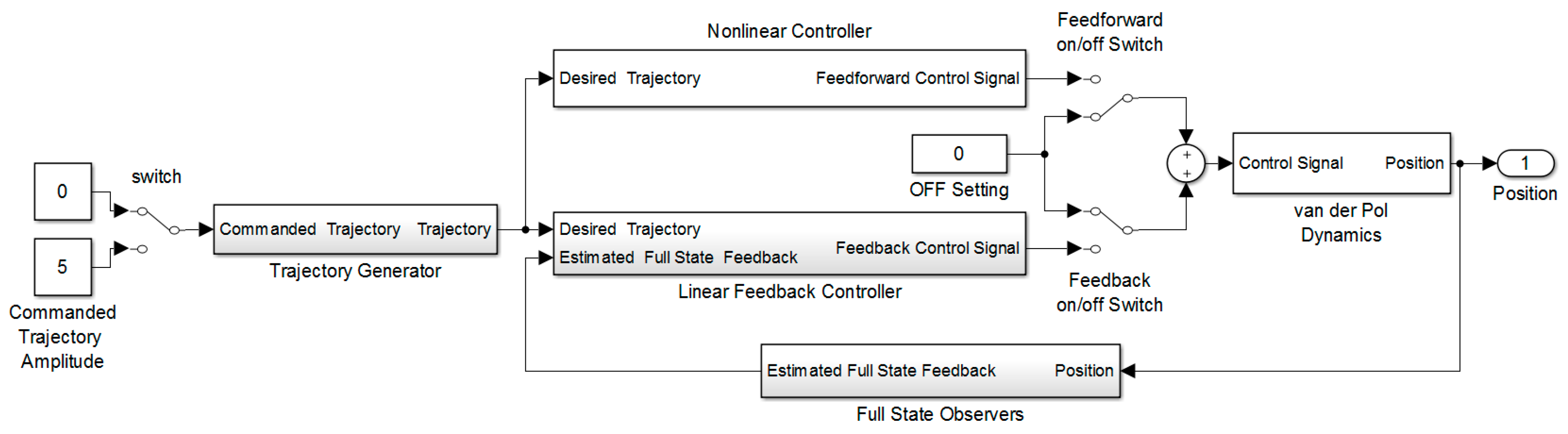
The methodology begins with elaboration of the inherent dynamics and impact of various initial conditions. Equation (1) is simulated in SIMULINK (Figure 1), where the nonlinear van der Pol equation is forward-propagated in time with various initial conditions. Figure 1 is the overall control topology coded in MATLAB/SIMULINK software (R2015b, Mathworks, 640 W California Ave, Sunnyvale, CA USA): Desired-trajectory (left) is fed to controllers (center) that formulate the forcing functions to drive the van der Pol dynamics (right). State observers are used to augment linear feedback controllers (but are not necessary for nonlinear feedforward controllers). Manual switches allow for “apples-to-apples” comparisons where all other features are kept constant except for the manually switched feature [5]. Results are plotted together on single plots to highlight relative behaviors. Then, controllers are designed and implemented in the same SIMULINK model. The dynamics after incorporation of the disparate controller varies. In the first instance to be examined, the dynamic remains open loop while using only an ideal nonlinear controller, while the second and third iterations include a linear, optimal feedback controller, and thus the system dynamics are closed-loop dynamics.
2.1. Inherent Dynamics
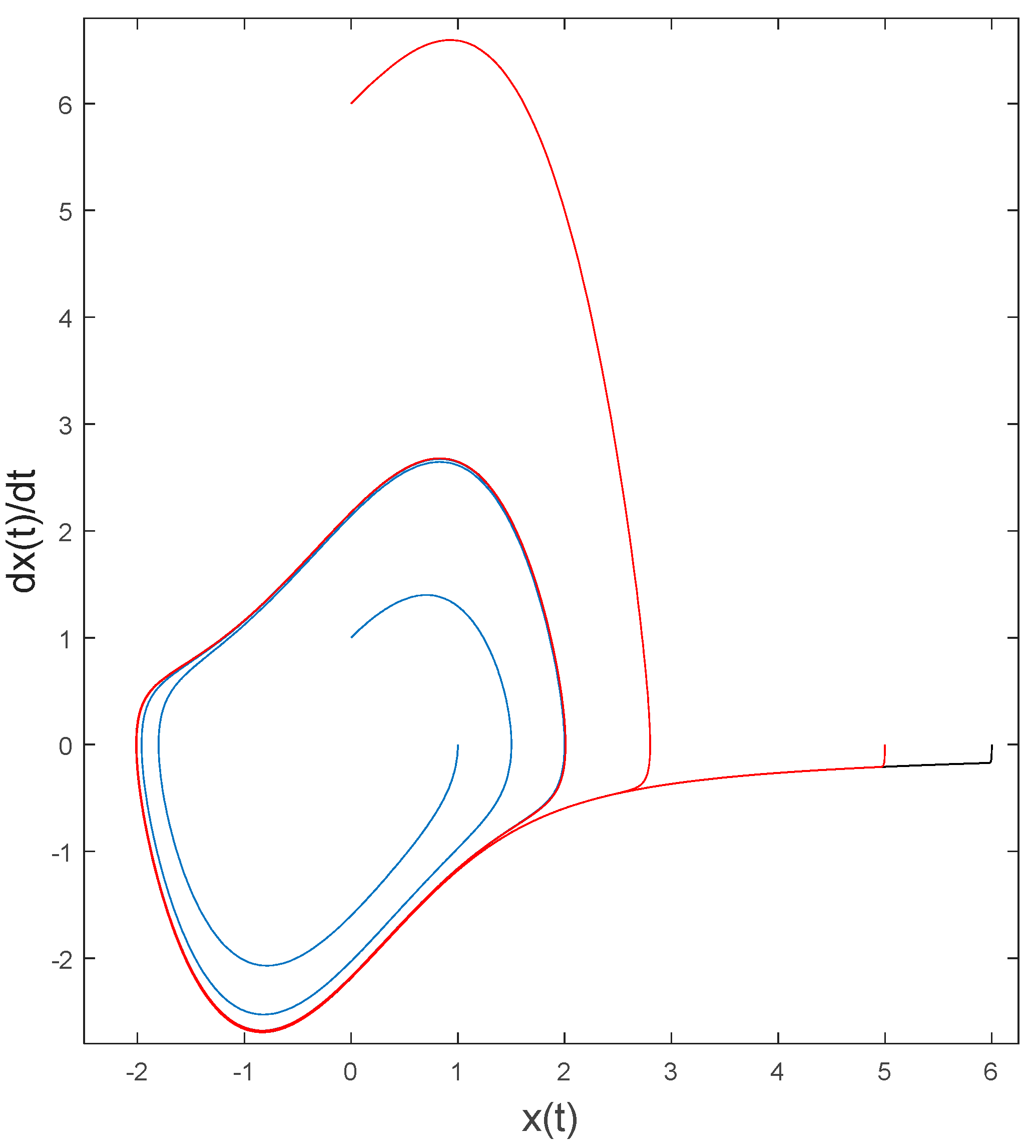
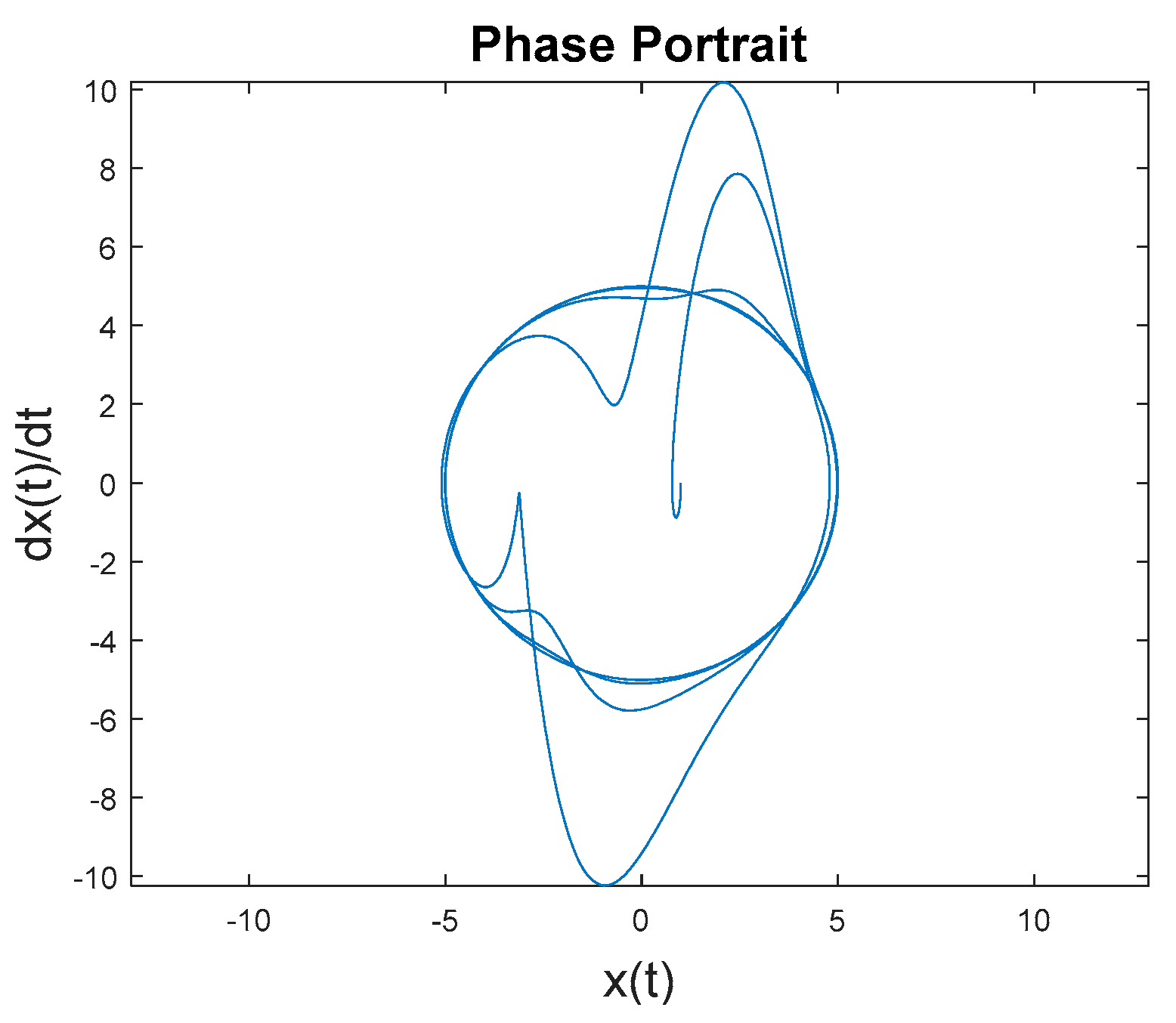
Figure 2 contains a visual depiction of the inherent dynamics for different intial conditions. Regardless of initial condition the governing equations trajectories converge to this invariant set.
2.2. Discussion of Initial Conditions
These initial conditions (Figure 2) are used for evaluation of various control schemes: optimal LTI feedback control, idealized feedforward control, and combined control using both of the aforementioned schemes. Figure 2 is a depiction of forward time-propagation of nonlinear van der Pol Equation (1) with several initial conditions chosen to demonstrate convergence to non-circular invariant set despite starting inside the set or outside the set.
2.3. Optimal Linear, Time-Invariant Feedback Control Design
The normal procedure for optimal LTI feedback control design is to linearize the governing system equation (the inherent dynamics), and then use the Ricatti equation to solve for optimal feedback gains (optimal with respect to the linearized dynamics), referred to as the LQR [6]. The identical process is valid for linear time-invariant observer design, although the result is referred to as linear quadratic estimator (LQE). This process is described in Section 3.2 and result in closed-loop dynamics.
2.4. Nonlinear Feedforward Control Design
The basic premise of idealized nonlinear feedforward control design [7,8,9] is to define the inherent dynamics as the idealized feedforward control (Equation (3)), where the control designer is required to specify the desired trajectory to be followed. In this study, the desired trajectory is a circle of constant-amplitude (a trajectory not producible by the inherent dynamics). The controller is idealized only with respect to the assumed parameter estimates (μ in Equation (1)). If those parameters were exactly known, the idealized control would seem perfect (although that is rarely or never the case, thus the rationale to investigate a combined control scheme of both idealized feedforward together with optimal feedback control). Equation (4) is merely a combined display of Equations (2) and (3). Equation (4) is the expression for the controlled dynamics after the controller is incorporated.
2.5. Analysis of the Ideal Nonlinear Controller
Perhaps the greatest strength of ideal nonlinear control is the simplicity of analysis. Merely equate coefficients order-of-differentiation in Equation (4) to see: , thus trajectory tracking is assured in steady state after the dissipation of the effects of initial conditions.
3. Results
The general methodology is to begin with basic scenarios, and then to change only one thing permitting the readers to understand the impact of the single change where the changes are incrementally added to eventually reveal a comparison of various control methodologies.
The van der Pol dynamics will be shown to converge to an invariant set (non-circular) at various initial conditions. Firstly, the desired trajectory will be commanded to stay at zero, despite no control activation. Next, a constant amplitude circular trajectory is commanded, and then an optimal linear time-invariant feedback controller will be used. Afterwards, the idealized feedforward control will be implemented followed lastly by the combined use of both optimal feedback control plus idealized nonlinear feedforward control.
3.1. Uncontrolled van der Pol Dynamic
3.1.1. Desired Trajectory Equals Zero
The initial simulation runs (Figure 1) commands a zero trajectory, but no control is activated. This simulation run establishes a baseline. Figure 3 depicts the initial baseline for evaluation. From a non-zero initial condition, the inherent dynamics will converge to a non-circular invariant set. This instance uses Figure 1 with a commanded zero trajectory, yet no control is activated (neither feedback nor feedforward). Figure 3 depicts the expected results: despite commanding zero trajectory, the system converges to the invariant set since no controllers are active. Figure 3a displays the baseline comparison of desired trajectory versus actual trajectory, while Figure 3b displays the state space trajectory (we will eventually seek to command this invariant set to be a circle of radius equal five).
3.1.2. Desired Trajectory Equals a Circular Oscillation (Baseline for Comparison of Forcing)
The next simulation run (Figure 1) commands a circular trajectory, but no control is activated. Figure 4 contains the first step away from the initial baseline for evaluation: Commanding a desired trajectory as a circle of radius five. From a non-zero initial condition, the inherent dynamics will converge to a non-circular invariant set. This instance uses Figure 1 with a commanded circular trajectory, yet no control is activated (neither feedback nor feedforward). Figure 4 depicts the expected results: despite commanding a circular trajectory, the system converges to the invariant set since no controllers are active. Figure 4a displays the baseline comparison of desired trajectory versus actual trajectory, while Figure 4b displays the state space trajectory (we’ll eventually seek to command this invariant set to be a circle of radius equal five using various controllers).
3.2. Van der Pol Dynamics Forced by Linear Feedback Controllers
3.2.1. Linearized van der Pol Equation Used for Linear Control Design
The normal first procedure for control design involves linearizing the dynamic equation, and afterwards designing the control signal using the linearized dynamics. Linearizing Equation (1) leads to Equation (5), expressed in state-variable formulation from which state space trajectories are displayed on phase portraits (e.g., Figure 2, Figure 3, Figure 4 and Figure 5).
[A] = [1 −1; 1; 0]; [B] = [−1; 0]; [C] = [0,1]; D = [0];
[Q]=[1 0; 0 1]; [R] = [1]; [S] = [2.6818 0.4142; 0.4142 3.3784]
Kp = 2.6818; Kd = 0.4142
Equations (5) and (6) are the expressions used in the linear-quadratic optimization leading to a feedback controller with proportional and derivative gains in Equation (7). The closed loop dynamics are established by Equation (2) where the van der Pol forcing function F(t) is a proportional-derivative (PD) controller per paragraph 8 in ref [10] who’s gains are in Equation (7) immediately above.
Equation (8) is the expression for the controlled dynamics after the linear optimal feedback controller (alone) is incorporated, while Equation (9) is the expression for the controlled dynamics after incorporation of both ideal nonlinear control together with linear optimal feedback control. Notice that in every instance the system is nonlinear, even in the instance of using only linear optimal feedback control (Equation (8)). The van der Pol differential equation is inherently nonlinear with a natural limit cycle that will be omnipresent in all dynamic equations of control of the van der Pol equation.
3.2.2. Linear Control Design
Finding optimal LTI feedback gains involves solving the Ricatti equation [11], whose details are not necessary to describe here, especially since it shall be immediately shown that such control is ineffective. MATLAB software can easily produce the optimal feedback gains with Equation (4) as input to the lqr(A,B,C,D) command, which tells MATLAB software to solve the linear-quadratic optimization problem. The results are Kp = 2.6818 and Kd = 0.4142, respectively, for the state (“position” subscripted p) and state derivative (derivative: subscripted d).
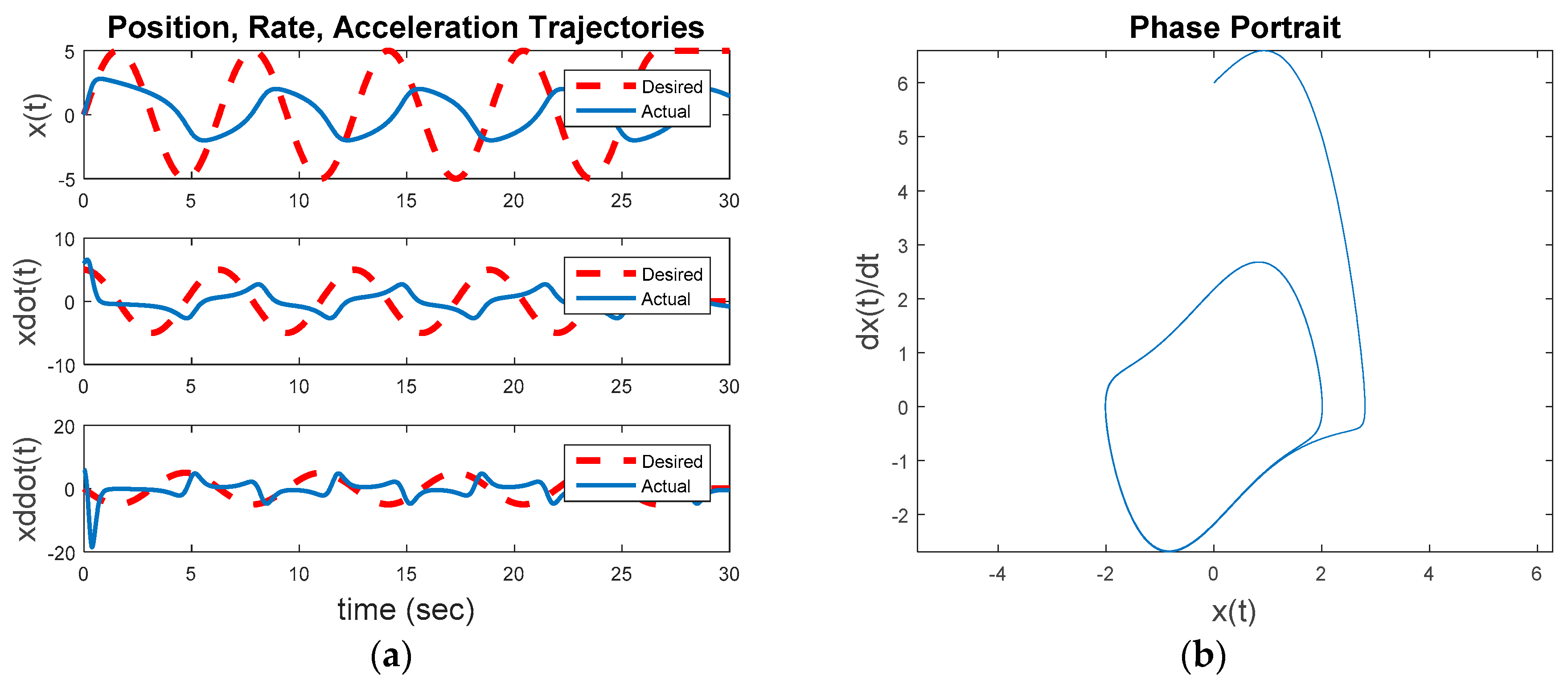
The next simulation run (Figure 1) commands a circular trajectory, with optimal LTI feedback control activated. The control is a LQR whose states are the position and derivative. Figure 5 depicts this second step away from the initial baseline for evaluation: Commanding a desired trajectory as a circle of radius five using optimal LTI feedback control. From a non-zero initial condition, the inherent dynamics will seek to converge to a non-circular invariant set while the feedback controller seeks to force the trajectory into a circle of radius equal to five. This instance uses Figure 1 with a commanded circular trajectory, and the control switch is activated for the feedback controller. Figure 5 depicts some interesting results. The commanded circular trajectory is not achieved with optimal LTI control. The nonlinear system converges to the invariant set regardless.
Figure 6a displays the baseline comparison of desired trajectory versus actual trajectory, while Figure 6b displays the position, rate, and acceleration errors. The bottom graph in Figure 6a reveals that while the optimal LTI control nearly closely replicates the desired acceleration trajectory, the errors in Figure 6b result in relatively large velocity errors displayed in the middle graph of Figure 6a, and subsequently large position errors displayed in the upper graph in Figure 6a. The optimal LTI feedback controller is not able to overcome the nonlinear inherent dynamics to achieve the commanded fixed-amplitude circular state space trajectory.
3.3. Van der Pol Dynamics Forced by only Nonlinear Feedforward Controllers
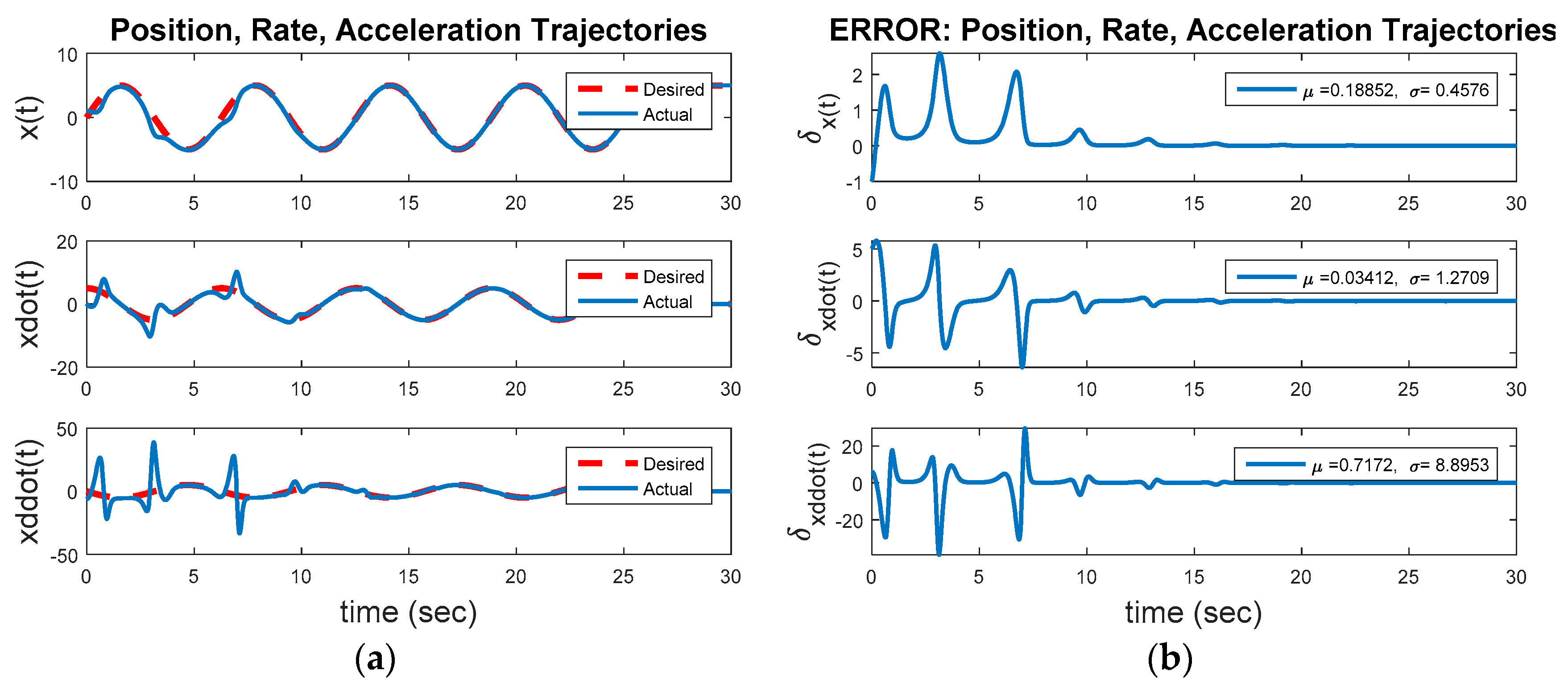
Figure 7 reveals the third step away from the initial baseline for evaluation: Commanding a desired trajectory as a circle of radius five using idealized feedforward control. From a non-zero initial condition, the inherent dynamics will seek to converge to a non-circular invariant set while the feedforward controller seek to force the trajectory into a circle of radius equal to five. This instance uses Figure 1 with a commanded circular trajectory, and the control switch is activated for the feedforward controller. Figure 7 reveals the idealized nonlinear feedforward controller designed per the methodology inspired by [7], implemented in [12] for Euler’s moment equations and augmented in [10,13], and demonstrated in [8,9]. The results of these steady improvements applied to the van der Pol equation results in Equation (4) which (after three-to-four overshoot events) achieves a circular oscillatory trajectory with the commanded amplitude. The result is obviously vastly superior to the results achieved with the optimal LTI feedback controller. Figure 8a displays the baseline comparison of desired trajectory versus actual trajectory (again revealing the overshoots followed by close trajectory following), Figure 8b displays the position, rate, and acceleration errors. Clearly visible in figure a, after the initial transient the idealized, nonlinear feedforward controller exactly achieves the commanded oscillatory trajectory, with very close command-following achieved after a short (10 s or so) startup transient.
3.4. Van der Pol Dynamics Forced by Both Linear Feedback and Nonlinear Feedforward Controllers
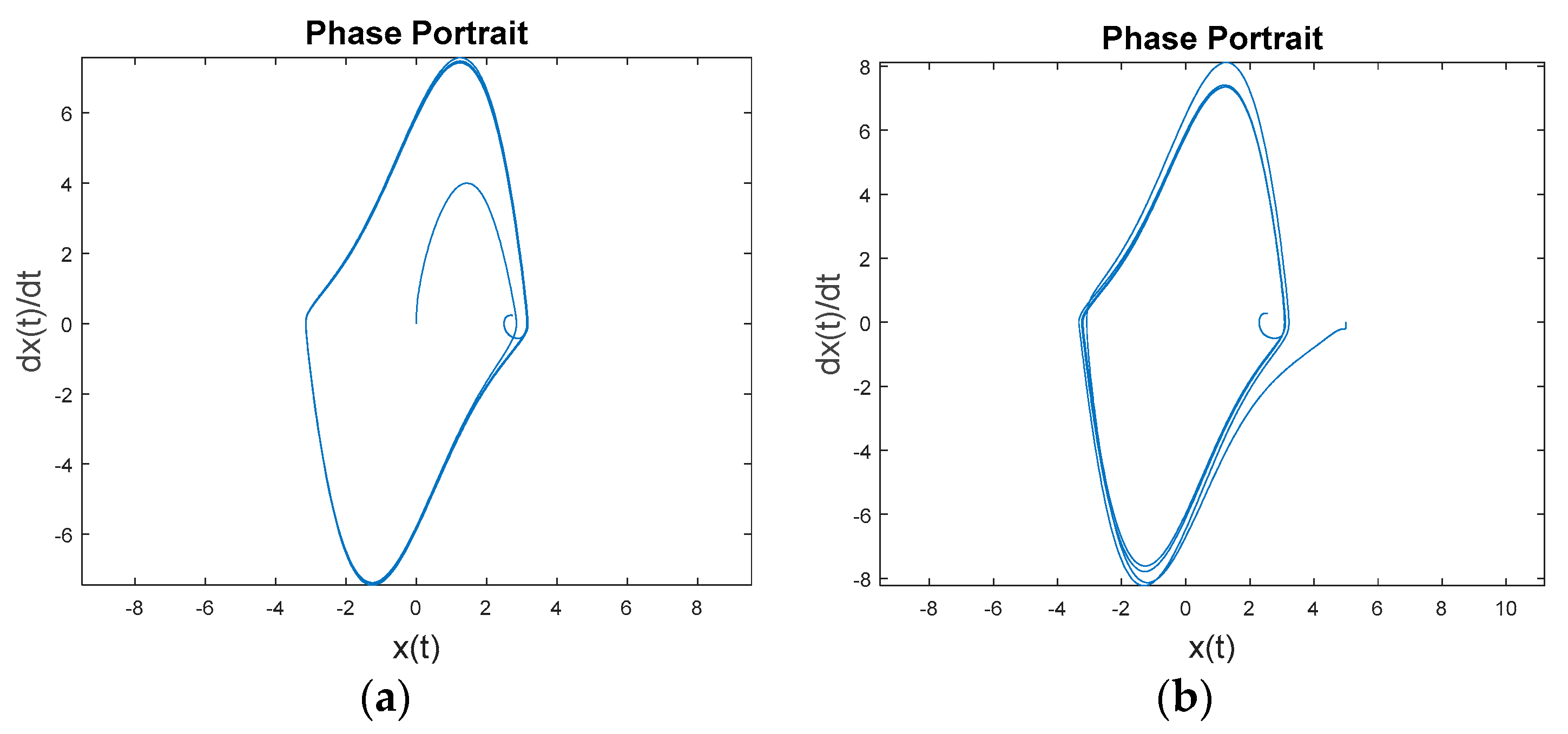
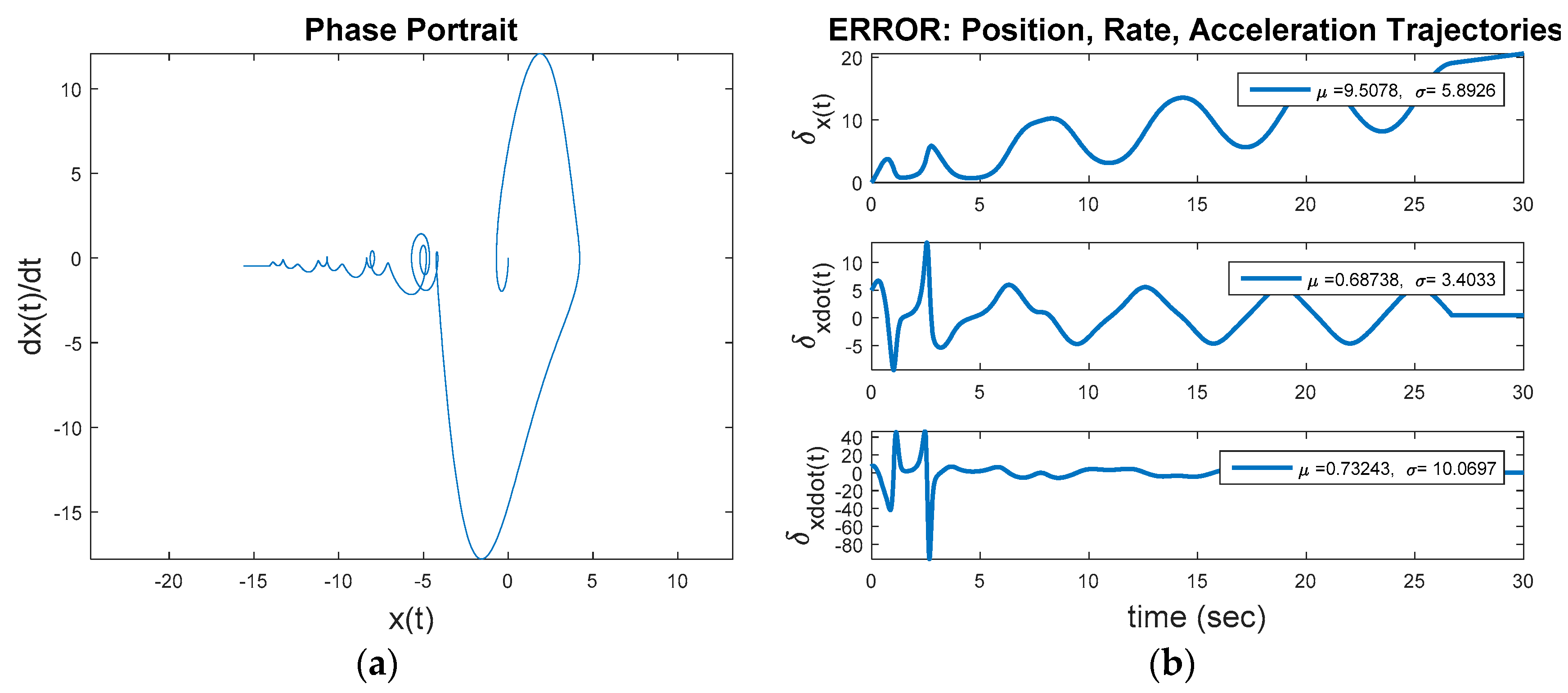
Figure 9 reveals the final iteration away from the initial baseline for evaluation: Commanding a desired trajectory as a circle of radius five using both idealized feedforward control and optimal linear, time-invariant feedback control. From a non-zero initial condition, the inherent dynamics will seek to converge to a non-circular invariant set while the feedforward controller seeks to force the trajectory into a circle of radius equal to five. The feedback controller also seeks the same goal, but was seen in earlier analysis not to be effective by itself. This instance uses Figure 1 with a commanded circular trajectory, and the control switch is activated for the feedforward controller. Figure 10 reveals the two components of control together are not effective. The idealized nonlinear feedforward controller (after three-to-four overshoot events) was shown earlier to achieve a circular oscillatory trajectory with the commanded amplitude (overcoming the inherent dynamics), but here we see the optimal linear, time-invariant controller interferes with that ability. The result is quite inferior to the results achieved with idealized nonlinear feedforward control alone. Figure 9b displays the position, rate, and acceleration errors. Despite achieving near-zero acceleration error after the initial transient, the resulting velocities and positions are already too far off and never achieve the commanded results.
4. Discussion
Section 3 Results revealed the general notion that idealized nonlinear feedforward control is the superior methodology, and this section elaborates those results with more detailed perspective and numerical interpretation. Analytical development was shown to very easy for ideal nonlinear control, and the following numerical results in terms of trajectory tracking error are emphasized. Low standard deviations are ubiquitous with idealized nonlinear control reinforcing the trajectory depictions in the previous sections. Table 1 displays the results of thirty simulation runs (Figure 1), where the only modification is the initial conditions and activation of the appropriate switch to engage the relevant control methodology.
Table 1 lists the mean errors, μ and standard deviations, σ for each of thirty simulation runs with various initial conditions and control methodologies with the most superior case listed in bold for each control methodology. The cases where the initial condition is on or inside the commanded circular amplitude, optimal LQR feedback control alone saw superior mean error (with greater standard deviation).
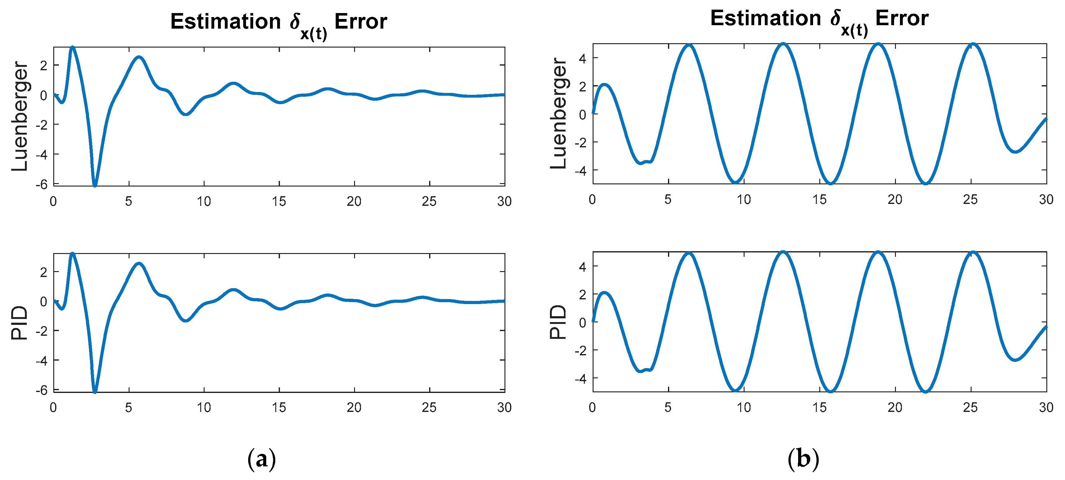
Another interesting thing to notice is the good ability of linear observers (both Luenberger-styled observers and PID observers) estimating the states [14,15,16] when the linear controller is active, yet the same observers perform very poorly when only the nonlinear control is active. Despite the superior trajectory-tracking performance of the nonlinear controller, the linear observer cannot estimate the states well.
Follow-on research: reacting to the very bad performance of the optimal LQR controller that was designed for a linearized version of the nonlinear van der Pol dynamics, future research will probe the question, “what can be done to linear optimal LQR feedback control to improve its performance with such nonlinear plants as van der Pol?” Additionally, auto-trajectory generation from the initial condition to the desired oscillatory manifold will be investigated in the sequel to eliminate the transient overshoots.
Author Contributions
All three authors performed the research used in this article. Corresponding author alone authored the text, while all three participated in editorial process.
Conflicts of Interest
The authors declare no conflict of interest.
References
- Van der Pol, B. A theory of the amplitude of free and forced triode vibrations. Radio Rev. 1920, 1, 701–710. [Google Scholar]
- Van der Pol, B. On “Relaxation Oscillations” I. Philos. Mag. 1926, 2, 978–992. [Google Scholar] [CrossRef]
- Van der Pol, B. The nonlinear theory of electric oscillations. Proc. IRE 1934, 22, 1051–1086. [Google Scholar] [CrossRef]
- Van der Pol, B.; van der Mark, J. Frequency de-multiplication. Nature 1927, 120, 363–364. [Google Scholar] [CrossRef]
- Van der Pol, B. Over Relaxatie-trillingen. Tijdschrift van het Nederlandsch Radiogenootschap 1926, 3, 25–40. [Google Scholar]
- Huibert, K.; Raphael, S. Linear Optimal Control Systems, 1st ed.; Wiley-Interscience: New York, NY, USA, 1972. [Google Scholar]
- Slotine, J. Applied Nonlinear Control; Prantice-Hall: Englewood Cliffs, NJ, USA, 1991; Chapter 9. [Google Scholar]
- Nakatani, S.; Sands, T. Autonomous Damage Recovery in Space. Int. J. Autom. Control Intell. Syst. 2016, 2, 31. [Google Scholar]
- Nakatani, S.; Sands, T. Simulation of Spacecraft Damage Tolerance and Adaptive Controls. In Proceedings of the 2014 IEEE Aerospace Proceedings, Big Sky, MT, USA, 1–8 March 2014. [Google Scholar]
- Sands, T. Physics-Based Control Methods. In Advances in Spacecraft Systems and Orbit Determination; Rushi, G., Ed.; In-Tech Publishers: Rijeka, Croatia, 2012; pp. 29–54. [Google Scholar]
- Gregory, C. Analysis and Control of Dynamic Economic Systems; John Wiley & Sons: New York, NY, USA, 1975. [Google Scholar]
- Heidlauf, P.; Cooper, M. Nonlinear Lyapunov Control Improved by an Extended Least Squares Adaptive Feed forward Controller and Enhanced Luenberger Observer. In Proceedings of the International Conference and Exhibition on Mechanical & Aerospace Engineering, Las Vegas, NV, USA, 2–4 October 2017. [Google Scholar]
- Sands, T. Fine Pointing of Military Spacecraft. Ph.D. Dissertation, Naval Postgraduate School, Monterey, CA, USA, 2007. [Google Scholar]
- Sands, T.; Lorenz, R. Physics-Based Automated Control of Spacecraft. In Proceedings of the AIAA Space 2009 Conference and Exposition, Pasadena, CA, USA, 14–17 September 2009. [Google Scholar]
- Sands, T. Improved Magnetic Levitation via Online Disturbance Decoupling. Phys. J. 2015, 1, 272–280. [Google Scholar]
- Sands, T. Phase Lag Elimination at All Frequencies for Full State Estimation of Spacecraft Attitude. Phys. J. 2017, 3. accepted. [Google Scholar]
Figure 1.
Overall control topology coded in MATLAB/SIMULINK software.

Figure 2.
Forward time-propagation of nonlinear van der Pol Equation (1).

Figure 3.
Initial baseline for evaluation. (a) Displays trajectory comparison; and (b) trajectory.

Figure 4.
Commanding a desired trajectory as a circle of radius five with no control activated (neither feedback nor feedforward): (a) displays trajectory comparison; and (b) trajectory.
Figure 4.
Commanding a desired trajectory as a circle of radius five with no control activated (neither feedback nor feedforward): (a) displays trajectory comparison; and (b) trajectory.

Figure 5.
Commanding a desired trajectory as a circle of radius five using optimal linear, time-invariant feedback control: (a) displays trajectory comparison; and (b) trajectory.
Figure 5.
Commanding a desired trajectory as a circle of radius five using optimal linear, time-invariant feedback control: (a) displays trajectory comparison; and (b) trajectory.

Figure 6.
Trajectory comparison and errors associate with Figure 5: (a) displays trajectory comparison; and (b) trajectory.
Figure 6.
Trajectory comparison and errors associate with Figure 5: (a) displays trajectory comparison; and (b) trajectory.

Figure 7.
Commanding a desired trajectory as a circle of radius five using idealized feedforward control.
Figure 7.
Commanding a desired trajectory as a circle of radius five using idealized feedforward control.

Figure 8.
Trajectory comparison and errors associate with Figure 7: (a) displays trajectory comparison; and (b) trajectory.
Figure 8.
Trajectory comparison and errors associate with Figure 7: (a) displays trajectory comparison; and (b) trajectory.

Figure 9.
Commanding a desired trajectory as a circle of radius five using both idealized feedforward control and optimal LTI feedback control. (a) displays trajectory comparison, (b) trajectory.
Figure 9.
Commanding a desired trajectory as a circle of radius five using both idealized feedforward control and optimal LTI feedback control. (a) displays trajectory comparison, (b) trajectory.

Figure 10.
(a) Estimation error using dual feedforward & feedback control. (b) Estimation error using only ideal, nonlinear feedforward control (notice poor estimation is not relevant since feedforward control does not use these estimates).
Figure 10.
(a) Estimation error using dual feedforward & feedback control. (b) Estimation error using only ideal, nonlinear feedforward control (notice poor estimation is not relevant since feedforward control does not use these estimates).


Table 1.
Comparison of forcing method (non-optimal observers). LQR.
| Initial Position | Unforced 1 | Forced by LQR Linear Feedback Kp = 1.1913 Kd = 0.9050 | Forced only by Idealized Nonlinear Feedforward |
|---|---|---|---|
| (0,0) | μ = 2.858 | μ = 0.28163 | μ = 0.083008 |
| σ = 3.357 | σ= 1.41 | σ = 0.30951 | |
| (5,0) | μ = 2.2539 | μ = 0.15107 | μ = −0.5283 |
| σ = 4.4174 | σ = 2.0607 | σ = 1.2645 | |
| (1,0) | μ = 2.8491 | μ = 0.28427 | μ = 0.092108 |
| σ = 3.4741 | σ = 1.4116 | σ = 0.33885 | |
| (0,1) | μ = 2.8756 | μ = 0.2784 | μ = 0.066252 |
| σ = 3.1283 | σ = 1.3977 | σ = 0.24343 | |
| (6,0) | μ = 1.7929 | μ = 0.0041396 | μ = −1.0166 |
| σ = 4.62 | σ = 2.9392 | σ = 2.0182 | |
| (0,6) | μ = 2.7794 | μ = 0.26159 | μ = 0.01697 |
| σ = 3.7424 | σ = 1.3979 | σ = 0.067415 |
1 Establishes baseline mean error, μ and standard deviation σ for comparison.
© 2017 by the authors. Licensee MDPI, Basel, Switzerland. This article is an open access article distributed under the terms and conditions of the Creative Commons Attribution (CC BY) license (http://creativecommons.org/licenses/by/4.0/).
Share and Cite
MDPI and ACS Style
Cooper, M.; Heidlauf, P.; Sands, T. Controlling Chaos—Forced van der Pol Equation. Mathematics 2017, 5, 70. https://0-doi-org.brum.beds.ac.uk/10.3390/math5040070
AMA Style
Cooper M, Heidlauf P, Sands T. Controlling Chaos—Forced van der Pol Equation. Mathematics. 2017; 5(4):70. https://0-doi-org.brum.beds.ac.uk/10.3390/math5040070
Chicago/Turabian StyleCooper, Matthew, Peter Heidlauf, and Timothy Sands. 2017. "Controlling Chaos—Forced van der Pol Equation" Mathematics 5, no. 4: 70. https://0-doi-org.brum.beds.ac.uk/10.3390/math5040070
Note that from the first issue of 2016, this journal uses article numbers instead of page numbers. See further details here.