Kinematics in the Information Age

Abstract

Modern kinematics derives directly from developments in the 1700s, and in their current instantiation, have been adopted as standard realizations…or templates that seem unquestionable. For example, so-called aerospace sequences of rotations are ubiquitously accepted as the norm for aerospace applications, owing from a recent heritage in the space age of the late twentieth century. With the waning of the space-age as a driver for technology development, the information age has risen with the advent of digital computers, and this begs for re-evaluation of assumptions made in the former era. The new context of the digital computer defines the use of the term “information age” in the manuscript title and further highlights the novelty and originality of the research. The effects of selecting different Direction Cosine Matrices (DCM)-to-Euler Angle rotations on accuracy, step size, and computational time in modern digital computers will be simulated and analyzed. The experimental setup will include all twelve DCM rotations and also includes critical analysis of necessary computational step size. The results show that the rotations are classified into symmetric and non-symmetric rotations and that no one DCM rotation outperforms the others in all metrics used, yielding the potential for trade space analysis to select the best DCM for a specific instance. Novel illustrations include the fact that one of the ubiquitous sequences (the “313 sequence”) has degraded relative accuracy measured by mean and standard deviations of errors, but may be calculated faster than the other ubiquitous sequence (the “321 sequence”), while a lesser known “231 sequence” has comparable accuracy and calculation-time. Evaluation of the 231 sequence also illustrates the originality of the research. These novelties are applied to spacecraft attitude control in this manuscript, but equally apply to robotics, aircraft, and surface and subsurface vehicles.

1. Introduction

The discipline of kinematics in its current form has a lengthy history that hark back to at least 1775 with Euler’s formulations [1], with almost immediate expansion throughout the nineteenth [2,3,4] and twentieth centuries [5,6,7,8,9,10,11,12,13,14,15,16,17,18,19,20,21,22,23,24,25,26,27,28,29]. There was a particular renaissance in the late twentieth century accompanying the race between the then-Soviet Union and the United States to spaceflight, and its accompanying application toward nuclear deterrence, where considerable lessons from that period (both technical and non-technical) have been expressed in subsequent literature [30,31,32,33,34,35,36,37,38,39,40,41,42,43,44,45,46,47,48,49,50,51,52,53,54,55,56,57,58,59,60,61,62]. From this distinguished lineage, terminology has converged to refer to sequential rotation sequences (e.g., xyz or 123); which are called aerospace sequences about non-repeating axes (also referred to as “Tait-Bryan angles”), while the orbit sequences have an axis repeated in the rotation sequence (e.g., xyx or 121, also referred to as “proper Euler angles”), [63]. One non-repeating sequence in particular (commonly called either a 321 or 123 sequence) has become the ubiquitous aerospace sequence. These cited manuscripts substantiate specific technical applications of the orbital and aerospace sequences, and those technical applications are the focus of this research in hopes of improved performance. With the rise of digital computation in the Information Age, this research critically evaluates the options (seeking diverging truths for the modern times) by addressing such questions as: Is the ubiquitous aerospace sequence (123 or alternatively 321) the best rotation sequence? Evaluation will be driven by two figures of merit: (1) mean and standard deviations of errors indicating how well each rotation sequence represents true roll, pitch, and yaw angles, and (2) computation time to reveals relative numerical superiority in the context of digital computers of the current state of the art. Analysis and results demonstrate the fact that 321 and 123 rotation sequences result in disparate errors and computation time, with the former being relatively superior. Furthermore, the 123 rotation was significantly slower than all the other rotations. Secondly, the symmetric rotations were on average slower than the non-symmetric rotations, despite the same mathematical process and number of steps to solve for the Euler Angles. Lastly, the fastest non-symmetric rotation was the 321 and the fastest symmetric was the 232, slightly faster than the 121 rotation. Taking all Direction Cosine Matrices (DCM) rotations into account, the 232 rotation was the fastest.

The significance of this research cannot be overstated. The current state of the art uses rotational sequences borne from a different era under a different paradigm, but the success of spaceflight has solidified those older results into the current psyche. This manuscript illustrates that improved errors and computational speed are both possible; and in keeping with the acceptance of the older paradigm by evolution of spaceflight, the context of this research is rotational mechanics [62] applied to spacecraft attitude control systems. These advancements complement advanced algorithms [37,38,39,40,41,42,43,44,45] for nonlinear adaptive system identification [55,56,57,58,59] and control [46,47,48,49,50,51,52,53,54] permitting improved performance of space missions [35,36,60] in a time when the United States has a pre-occupation with low-end conflicts in the middle east amidst an increasing belligerent world of threats [30,31,32,33,34]. This realization culminated in the recent edict to create a new military service in the US. purely dedicated to space [61].

2. Materials and Methods

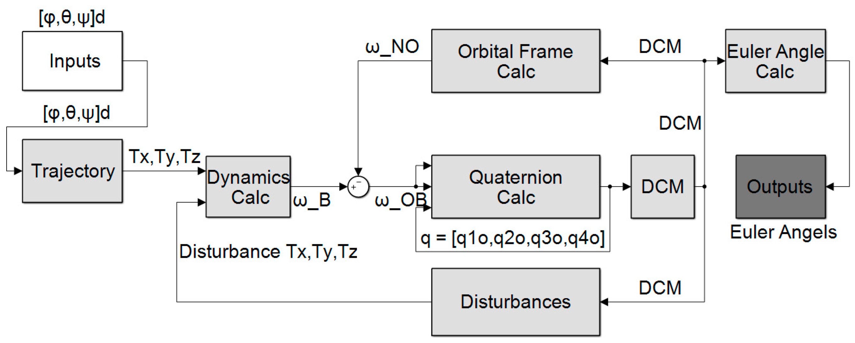
The goal of a spacecraft’s Attitude Control System (ACS) is to have a functional system that can move to and hold a specific orientation in three dimensional space, relative to an inertial frame. With regard to classical and rigid body mechanics, the ACS takes into account the Kinetics, Kinematics, Orbital Frame, and Disturbances to control this motion. Figure 1 depicts this process and details the computational steps from desired angle inputs to Euler Angle outputs in the sequence of inputs (from the white blocks in Figure 1) through light grey calculations to dark grey outputs: φ, θ, and ψ. Section 2 will explain the theory behind this control system, Section 3 will detail the experimental setup, and Section 4 will show the results and analysis.

2.1. Theory of Dynamics

Dynamics is synonymous with Mechanics. Newton called dynamics the science of machines which may be divided into two parts: statics (later called kinematics) and kinetics [2]. Chasle’s Theorem articulates how a complete description of motion may be described as a screw displacement comprised of translation in accordance with Newton’s Law and rotations in accordance with Euler’s Moment Equations $T=J\dot{\omega }+\omega \times J\omega$ [6], where [$J$] is a matrix of mass moments of inertia explained by Kane [23]. Investigation of motion without consideration of the nature of the body that is moved or how the motion is produced is called Phoronomics, or “the laws of going”, or more commonly but less properly kinematics [13], to be elaborated in Section 2.1.2. The rotation maneuver from one position to another is measured from the inertial reference frame or [X_I, Y_I, Z_I] to the final position, the body reference frame or [X_B, Y_B, Z_B]. For this simulation, a model was created to rotate from orientation A, [X_A, Y_A, Z_A] to orientation B, [X_B, Y_B, Z_B]. Since the dot product of two unit vectors is the cosine of the angle between them [25], it is referred to in older works as a direction cosine, which may also be used to describe a satellite in an inclined earth orbit [17] or to express the orientation of the perifocal reference frame with respect to the geocentric-equatorial reference frame [26]. Direction angles are the angles between each coordinate axis and the individual components of the vector. The direction cosines are simply the cosines of these angles [28]. The nature of direction cosines matrices is merely to assemble the direction cosines which completely specify the relative orientation of two coordinate systems [18], thus their appeal as universally applicable tools of kinematics.

2.1.1. Kinetics

Kinetics, or Dynamics, is the process of describing the motion of objects with focus on the forces involved. In the inertial frame, Newton’s $F=ma$ is applied but becomes Euler’s $T=J\dot{\omega }$ when rotation is added, where $T=J\dot{\omega }$ is expressed in the inertial reference frame’s coordinates, while $T=J\dot{\omega }+\omega \times J\omega$ from above is still measured in the inertial frame, but expressed in body coordinates.

Combining the Euler and Newton equations, we can account for all six degrees of freedom. In application, when an input angle [φ_d, θ_d, ψ_d] is commanded, the feedforward control uses (1) as the ideal controller with (2) as the sinusoidal trajectory to calculate the required torque [$T_x,T_y,T_z$] necessary to achieve the desired input angle. The Dynamics calculator then uses (3) to convert the torques into ω_B values, where ω_B is defined as the angular velocity of the body. In order to calculate this, the non-diagonal terms in (4) are neglected, removing coupled motion and leaving only the principle moments of inertia. Then, the inertia matrix J is removed from $J\dot{\omega }$, and the remaining $\dot{\omega }$ is integrated into [${\omega }_x,{\omega }_y,{\omega }_z]$, which is fed into the Kinematics block of the model to finally determine the outputted Euler Angles.

$$T_d=J{\dot{\omega }}_d+{\omega }_d\times J{\omega }_d$$

(1)

$$\theta =\frac{1}{2}\left(A+Asin\left({\omega }_{f}t+\phi \right)\right)$$

(2)

$$T={\dot{H}}_i=J{\dot{\omega }}_i+{\omega }_i\times J{\omega }_i$$

(3)

2.1.2. Kinematics, Phoronomics, or “The Laws of Going”

Formulation of spacecraft attitude dynamics and control problems involves considerations of kinematics, especially as it pertains to the orientation of a rigid body that is in rotational motion. The subject of kinematics is mathematical in nature, because it does not involve any forces associated with motion. The kinematic representation of the orientation of one reference frame relative to another reference can also be expressed by introducing the time-dependence of Euler Angles. The so-called body-axis rotations involve successive rotations three times about the axes of the rotated body-fixed reference frame resulting in twelve possible sets of Euler angles. The so-called space-axis rotations instead involve three successive rotations using axes fixed in the inertial frame of reference, again producing twelve possible sets of Euler angles. Because the body-axis and space-axis rotations are intimately related, only twelve Euler angle possibilities need be investigated; and the twelve sets from the body-axis sequence are typically used [26]. Consider a rigid body fixed at a stationary point whose inertia ellipsoid at the origin is an ellipsoid of revolution whose center of gravity lies on the axis of symmetry. Rotation around the axis of symmetry does not change the Lagrangian function, so there must-exist a first integral which is a projection of an angular momentum vector onto the axis of symmetry. Three coordinates in the configuration space special orthogonal group (3) may be used to form a local coordinate system, and these coordinates are called the Euler angles.

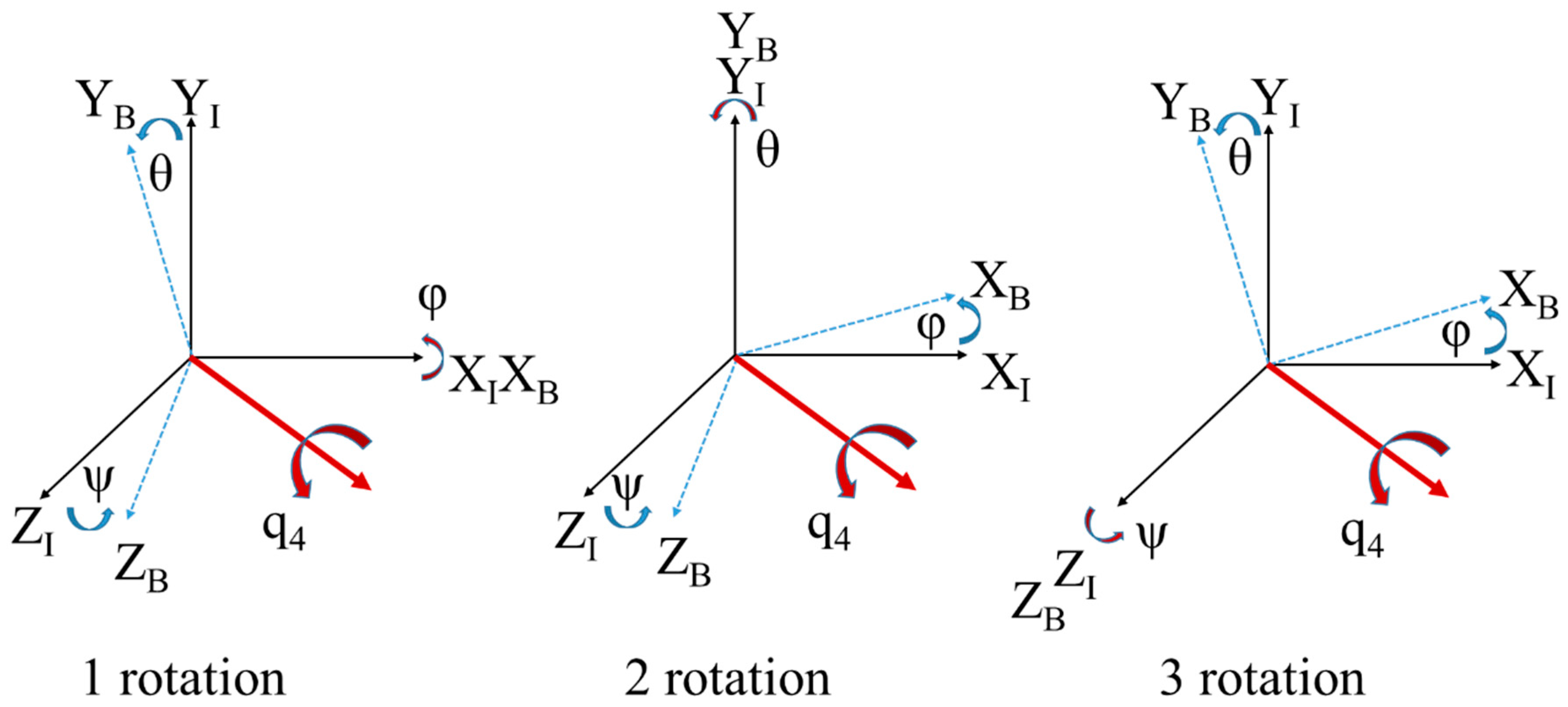
Key tools of kinematics from which the Euler angles may be derived include direction cosines which describe orientation of the body set of axes relative to an external set of axes. Euler’s angles may be defined by the following set of rotations: “rotation about x axis by angle and θ, rotation about z’ axis by an angle ψ, then rotation about the original z-axis by angle φ”. Eulerian angles have several “conventions: Goldstein uses [22] the “x-convention”: z-rotation followed by x’ rotation, followed by z’ rotation (essentially a 3-1-3 sequence). Quantum mechanics, nuclear physics, and particle physics the “y-convention” is used: essentially a 3-2-3 rotation). Both of these have drawbacks, that the primed coordinate system is only slightly different than the unprimed system, such that, φ and ψ become indistinguishable, since their respective axes of rotation (z and z’) are nearly coincident. The so-called Tait-Bryan convention in Figure 2 therefore gets around this problem by making each of the three rotations about different axes: (essentially a 3-2-1 sequence) [22].

Kinematics is the process of describing the motion of objects without focus on the forces involved. The [${\omega }_x,{\omega }_y,{\omega }_z$] values from the Dynamics are fed into the Quaternion Calculator where (5) and (6) yield q, the Quaternion vector. The Quaternions define the Euler axis in three dimensional space using [q₁, q₂, q₃]. About this axis, a single angle of rotation [q₄] can resolve an object aligned in reference frame A into reference frame B. The Direction Cosine Matrix (DCM) then relates the input ω values to the Euler Angles using one of 12 permutations of possible rotation sequences, where multiple rotations can be made in sequence. Therefore, the rows of the DCM show the axes of Frame A represented in Frame B, the columns show the axes of Frame B represented in Frame A, and φ, θ, and ψ are the angles of rotation that must occur in each axis sequentially to rotate from orientation A to orientation B, turning C^A to C^B. Figure 2 depicts a 3-2-1 sequence to rotate from C^A to C^B, where the Euler Axis is annotated by the thickest line.

$$\left[\begin{array}{c}{J}_{xx}{\dot{\omega }}_x+J_{xy}{\dot{\omega }}_y+J_{xz}{\dot{\omega }}_z-J_{xy}{\omega }_x{\omega }_z-J_{yy}{\omega }_y{\omega }_z-J_{yz}{\omega }_z^2+J_{xz}{\omega }_x{\omega }_y+J_{zz}{\omega }_z{\omega }_y+J_{yz}{\omega }_y^2\\ J_{yx}{\dot{\omega }}_x+J_{yy}{\dot{\omega }}_y+J_{yz}{\dot{\omega }}_z-J_{yz}{\omega }_x{\omega }_y-J_{zz}{\omega }_x{\omega }_z-J_{xz}{\omega }_x^2+J_{xx}{\omega }_x{\omega }_z+J_{xy}{\omega }_z{\omega }_y+J_{xz}{\omega }_z^2\\ J_{zx}{\dot{\omega }}_x+J_{zy}{\dot{\omega }}_y+J_{zz}{\dot{\omega }}_z-J_{xx}{\omega }_x{\omega }_y-J_{xz}{\omega }_y{\omega }_z-J_{xy}{\omega }_y^2+J_{yy}{\omega }_x{\omega }_y+J_{yz}{\omega }_z{\omega }_x+J_{xy}{\omega }_x^2\end{array}\right]=\left[\begin{array}{c}{T}_x\\ T_y\\ T_z\end{array}\right]$$

(4)

$$\left[\begin{array}{c}{\dot{q}}_1\\ {\dot{q}}_2\\ {\dot{q}}_3\\ {\dot{q}}_4\end{array}\right]=\frac{1}{2}\left[\begin{array}{cccc}0& {\omega }_3& -{\omega }_2& {\omega }_1\\ -{\omega }_3& 0& {\omega }_1& {\omega }_2\\ {\omega }_2& -{\omega }_1& 0& {\omega }_3\\ -{\omega }_1& -{\omega }_2& -{\omega }_3& 0\end{array}\right]\left[\begin{array}{c}{q}_1\\ q_2\\ q_3\\ q_4\end{array}\right]=\frac{1}{2}\left[\begin{array}{cccc}{q}_4& -q_3& q_2& q_1\\ q_3& q_4& -q_1& q_2\\ -q_2& q_1& q_4& q_3\\ -q_1& -q_2& -q_3& q_4\end{array}\right]\left[\begin{array}{c}{w}_1\\ w_2\\ w_3\\ 0\end{array}\right]$$

(5)

$$\left[\begin{array}{ccc}1-2\left(q_2^2+q_3^2\right)& 2\left(q_1{q}_2+q_3{q}_4\right)& 2\left(q_1{q}_3-q_2{q}_4\right)\\ 2\left(q_2{q}_1-q_3{q}_4\right)& 1-2\left(q_1^2+q_3^2\right)& 2\left(q_2{q}_3+q_1{q}_4\right)\\ 2\left(q_3{q}_1+q_2{q}_4\right)& 2\left(q_3{q}_2-q_1{q}_4\right)& 1-2\left(q_1^2+q_2^2\right)\end{array}\right]=\left[\begin{array}{ccc}{C}_2{C}_3& C_2{S}_3& -S_2\\ S_1{S}_2{C}_3-C_1{S}_3& S_1{S}_2{S}_3+C_1{C}_3& S_1{C}_2\\ C_1{S}_2{C}_3-S_1{S}_3& C_1{S}_2{S}_3-S_1{C}_3& C_1{C}_2\end{array}\right]$$

(6)

2.1.3. The Orbital Frame

In order to more completely represent a maneuvering spacecraft, orbital motion must be included with the Kinematics. This relationship is represented in Figure 1, where the output of the DCM is fed into the Orbital Frame Calculator, and the second column of the DCM is multiplied against the orbital velocity of the spacecraft. The second column of the DCM represents the Y axis of Frame B projected in the X, Y, and Z axes of Frame A. This yields ${\omega }^{NO}$, the orbital velocity relative to the Inertial Frame. Using (7), this velocity is removed from the velocity of the body relative to the Inertial Frame, leaving only the velocity of the body relative to the Orbital Frame for further calculations.

$${\omega }^{OB}={\omega }^{NB}-{\omega }^{NO}$$

(7)

2.1.4. Disturbances

Multiple disturbances torques exist that effect the motion of a spacecraft in orbit, two of which are addressed in this paper. The first is the disturbance due to gravity acting upon an object in orbit, where the force due to gravity decreases as the distance between objects increases. The force is applied as a scaling factor to the mass distribution around the Z axis of a spacecraft. This force applied to a mass offset from the center of gravity is calculated through the cross product found in (8) and yields an output torque about the Z axis.

The second disturbance is an aerodynamic torque due to the force of the atmosphere acting upon a spacecraft, which also decreases as the altitude increases. In (9), the force due to air resistance is calculated by scaling the direction of orbital velocity by the atmospheric density, drag coefficient, and magnitude of orbital velocity. This force then acts upon the center of pressure, which is offset from the center of gravity, and yields a torque about the Z axis, due to the cross product in (9).

The disturbances are additive and act upon the dynamics in Figure 1. Because the ideal feedforward controller is the dynamics, an offsetting component equal to the negative anticipated disturbances can be used to negate the disturbance torque. This results in nullifying the disturbances when the two are summed to produce ${\omega }^{OB}$, the velocity of the body relative to the Inertial Frame.

$$T_g=3\frac{\mu }{R^3}\widehat{z}\times J\widehat{z}$$

(8)

$$T_a=C_p\times f_a=C_p\times \left[\left({\rho }_a{V}_R{}^2{A}_p\right){\widehat{V}}_R\right]$$

(9)

2.2. Experimental Setup

This experiment implemented and compared the 12 DCM to Euler Angle rotations using a variable step size. An angle of [φ, θ, ψ] = [30, 0, 0] was commanded, with the quaternion and torques initialized as T = [0, 0, 0] and q = [0, 0, 0, 1]. The spacecraft had an inertia matrix of J = [2, 0.1, 0.1; 0.1, 2, 0.1; 0.1, 0.1, 2]. The orbital altitude was set at 150 km with a drag coefficient of 2.5. Both orbital motion and torque disturbances were turned off.

Each simulation executed over a 5 s quiescent period, 5 s maneuver time, and 5 s post maneuver observation period, totaling 15 s. The sinusoidal trajectory was calculated to have ${\omega }_f=\pi /2$ and $\phi =\pi /2$.

The model was built in Matlab and Simulink, where integrations were calculated using the Runge–Kutta solver (ode4) with variable time steps of 0.1, 0.001, and 0.0001 s. Euler Angles were resolved using the 12 unique DCM rotation sequences with the atan2 function.

Three Figures of Merit were used to assess performance. The first two were the mean and standard deviation between the Euler Angles and Body Angles. The third was the calculation time for each rotation as a measure of complexity.

3. Experimental Results and Analysis

3.1. Euler Angle Calculations and Post-Processing

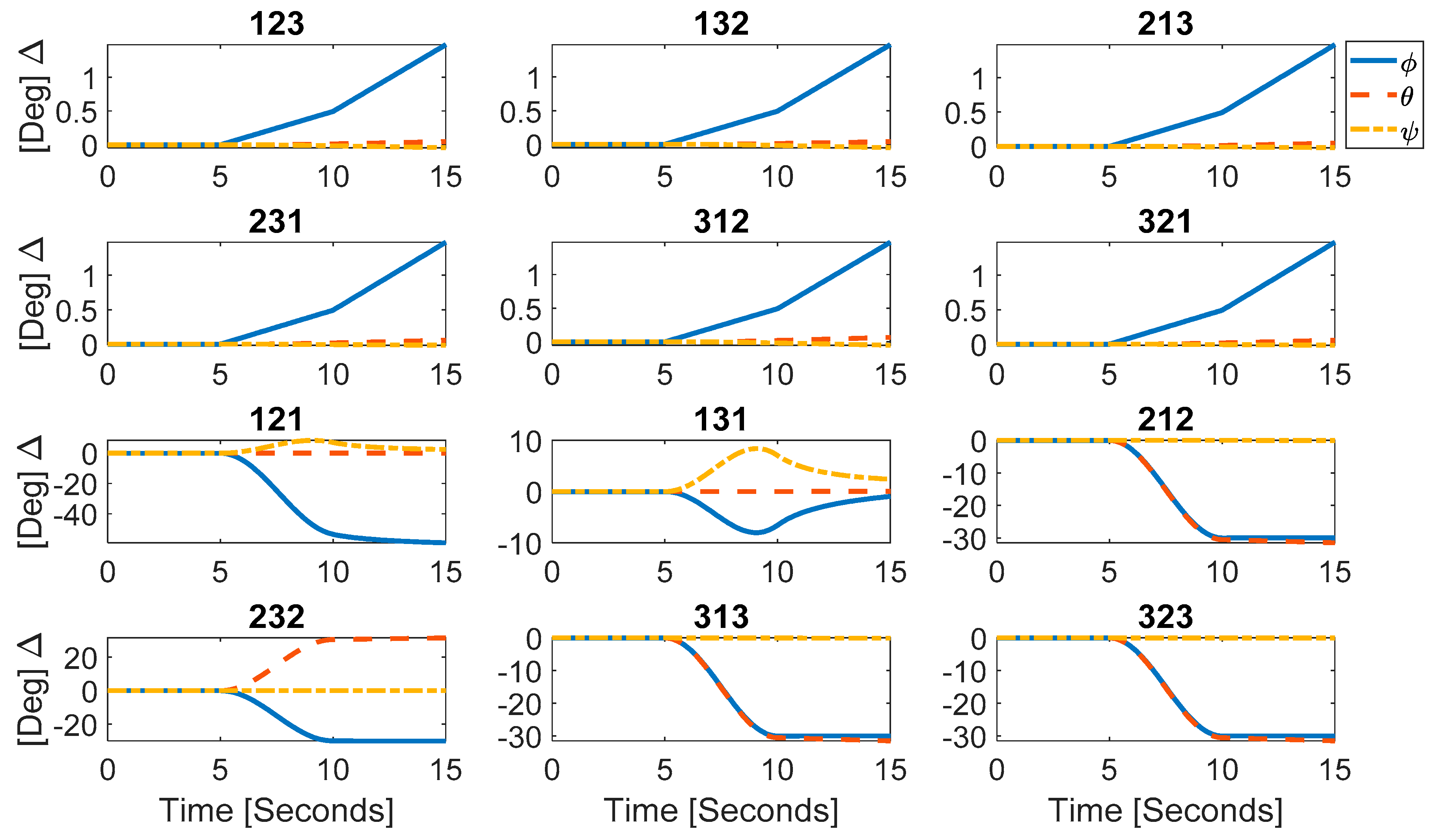
Each of the Euler angles was derived using the DCM and rotation matrices, creating a relationship like (7), but unique to each rotation. φ, θ, and ψ were isolated in this relationship as a method to calculate the Euler Angles. Once calculated, the Euler Angles were implemented in the simulation. However, when a [30, 0, 0] maneuver was commanded, discontinuities due to trigonometric quadrant error manifested. Post-processing removed the error, but yielded output rotation did not match the input command. In order to correct this, the derivations for each Euler Angle were revised to correlate six of the 12 rotations, yielding the results in Figure 3. Therefore, the rotations in Figure 3 are classified into two groups: the upper six non-symmetric rotations and lower six symmetric rotations. An example of symmetric rotations is 121, while a 132 is non-symmetric rotation. The commanded input and output maneuvers were not correlated for the 6 symmetric rotations.

3.2. Euler Angle to Body Angle Accuracy

The output Euler Angles are not the same as the commanded Body Angles, but measuring this delta is a method of determining accuracy. Figure 4 depicts the deviation over time and

Table 1. Mean and standard deviation for all 12 rotations, using a 0.1 step size.

	Mean			Standard Deviation
DCM	ϕ	θ	ψ	ϕ	θ	ψ
123	0.413	0.011	0.011	0.462	0.015	0.014
132	0.413	0.010	0.013	0.462	0.013	0.016
213	0.413	0.011	0.005	0.462	0.015	0.006
231	0.413	0.014	0.005	0.462	0.018	0.005
312	0.413	0.016	0.013	0.462	0.021	0.016
321	0.413	0.014	0.005	0.462	0.018	0.005
121	27.544	0.015	2.869	25.804	0.019	2.823
131	2.456	0.015	2.869	2.680	0.019	2.823
212	14.977	15.413	0.010	13.726	14.150	0.010
232	15.010	15.413	0.010	13.757	14.150	0.010
313	14.980	15.413	0.028	13.728	14.150	0.034
323	14.977	15.413	0.010	13.725	14.150	0.010

provides the associated mean values and standard deviations for each of the rotations.

The six non-symmetric rotations show consistent error in φ, and only begin to deviate beyond the fifth decimal place in both mean error and standard deviation. While φ is commanded to change to 30°, θ and ψ are expected to remain at zero, but show non-zero values due to error incurred by step size.

The six symmetric rotations are substantially harder to draw conclusions from because of the uncorrelated rotations. The mean error and standard deviation values are drastically different from each other in Table 1 and visibly deviate in Figure 4. Therefore, further correlation is required to analyze accuracy. Table 1 values were calculated over the 15 s simulation time, noting that some sequences had not reached steady-state values making their error values even larger compared to others in Table 1 if the simulations has been run until steady state was reached.

3.3. Step Size Versus Accuracy

The simulation step size was altered to determine the effects on accuracy for the 12 rotations. If variable step-size were used, there would be no way to assure a certain level of accuracy, thus fixed step size was utilized and iterated smaller-and-smaller until no discernable accuracy improvement is noted. Figure 5 shows the results of reducing the step size from 0.1 to 0.001 s. Figure 4 and Figure 5 remain comparable, with the ${10}^2$ order of magnitude decrease in step size yielded a comparable ${10}^2$ order of magnitude increase in accuracy. When a step size of 0.0001 s was used, the accuracy increased by another order of magnitude, denoting the trend. Comparing against the accuracy of the rotations, they maintained their relative accuracy; the 132 and 312 remained the most accurate rotations when the step size decreased, and therefore has limited to no effect.

3.4. DCM to Euler Angle Timing

The execution time of each maneuver was standardized at 15 s across all scenarios. Therefore, runtime deviations for each of the 12 rotations are attributable to the complexity of the calculations.

Table 2. Simulation run times for all 12 Direction Cosine Matrices (DCM) rotations for a 30° roll maneuver, using 0.1, 0.001, and 0.0001 step sizes.

	Simulation Execution Time [S]
DCM	0.1 Step size	0.001 Step size	0.0001 Step size
123	8.408	11.836	28.433
132	1.533	6.789	22.187
213	1.419	6.978	22.102
231	1.188	4.436	23.259
312	1.549	4.302	20.971
321	1.018	3.475	21.420
121	0.952	3.715	20.505
131	1.190	4.082	23.331
212	1.015	3.860	21.005
232	0.931	3.710	21.410
313	0.939	3.789	20.908
323	1.091	3.955	22.044

shows the results for three different step sizes and the runtimes for each rotation. Because the step size affected the simulation timing, comparisons were only valid between rotations of a similar step size; however, relative comparisons between step sizes were valid.

Analyzing the results yields several observations. Firstly, the 123 rotation was significantly slower than all the other rotations. Secondly, the symmetric rotations were on average slower than the non-symmetric rotations, despite the same mathematical process and number of steps to solve for the Euler Angles. Lastly, the fastest non-symmetric rotation was the 321 and the fastest symmetric was the 232, slightly faster than the 121 rotation. Taking all DCM rotations into account, the 232 rotation was the fastest.

4. Conclusions

This experiment implemented and compared the 12 DCM to Euler Angle rotations using a variable step size. The effects on accuracy, step size, and timing were observed, and the simulation results showed that the DCMs were classified into symmetric and non-symmetric rotations. The non-symmetric rotations were easier to correlate and compare, while the symmetric rotations were not, limiting analysis. Furthermore, no one rotation was the ideal in the analyzed categories. This is beneficial, because trade space analysis can be conducted to determine accuracy, timing, and other high priority design criteria to select the appropriate DCM. The lowest roll mean error is obtained by using any of the 123, 132, 213, 231, 312, or 321 rotation sequences, while the lowest pitch mean error cannot be achieved by the ubiquitous 321 sequence, instead the 132 sequence must be used; while the lowest yaw mean error may be achieved with the 213, 231, and 321 sequences. Standard deviations show similar options for selecting different rotation sequences for specific applications. Regarding computational efficiency, the 232 sequence was best, followed by the 313, and then the 121 sequence. The ubiquitously accepted standard 321 sequence was found to be fifth fastest, with four other rotation sequences bearing less computational burden. Novel illustrations include the fact that one of the ubiquitous sequences (the “313 sequence”) has degraded relative accuracy measured by mean and standard deviations of errors, but may be calculated faster than the other ubiquitous sequence (the “321 sequence”), while a lesser known “231 sequence” has comparable accuracy and calculation-time. Evaluation of the 231 sequence also illustrates the originality of the research. These novelties are applied to spacecraft attitude control in this manuscript, but can equally be applied to robotics, aircraft, and surface and subsurface vehicles.

Lastly, future research would refine the correlation for symmetric rotations, but furthermore experimental validation will be performed on free-floating spacecraft simulator hardware at the Naval Postgraduate School. The validation will be performed by duplicating one of the specifically cited technical applications (e.g., any of the technical applications in [35,36,37,38,39,40,41,42,43,44,45]) seeking to validate performance improvement.

References

- Euler, L. (Euler) Formulae Generales pro Translatione Quacunque Corporum Rigidorum (General Formulas for the Translation of Arbitrary Rigid Bodies), Presented to the St. Petersburg Academy on 9 October 1775. and First Published in Novi Commentarii Academiae Scientiarum Petropolitanae 20, 1776, pp. 189–207 (E478) and Was Reprinted in Theoria motus corporum rigidorum, ed. nova, 1790, pp. 449–460 (E478a) and Later in His Collected Works Opera Omnia, Series 2, Volume 9, pp. 84–98. Available online: https://math.dartmouth.edu/~euler/docs/originals/E478.pdf (accessed on 22 August 2018).
- Thompson, W.; Tait, P.G. Elements of Natural Philosophy; Cambridge University Press: Cambridge, UK, 1872. [Google Scholar]
- Reuleaux, F.; Kennedy Alex, B.W. The Kinematics of Machinery: Outlines of a Theory of Machines; Macmillan: London, UK, 1876; Available online: https://archive.org/details/kinematicsofmach00reuluoft (accessed on 22 August 2018).
- Wright, T.W. Elements of Mechanics Including Kinematics, Kinetics and Statics; D. Van Nostrand Company: New York, NY, USA; Harvard University: Cambridge, MA, USA, 1896. [Google Scholar]
- Merz, J.T. A History of European Thought in the Nineteenth Century; Blackwood: London, UK, 1903; p. 5. [Google Scholar]
- Whittaker, E.T. A Treatise on the Analytical Dynamics of Particles and Rigid Bodies; Cambridge University Press: Cambridge, UK, 1904. [Google Scholar]
- Whittaker, E.T. A Treatise on the Analytical Dynamics of Particles and Rigid Bodies; Cambridge University Press: Cambridge, UK, 1917. [Google Scholar]
- Whittaker, E.T. A Treatise on the Analytical Dynamics of Particles and Rigid Bodies; Cambridge University Press: Cambridge, UK, 1927. [Google Scholar]
- Whittaker, E.T. A Treatise on the Analytical Dynamics of Particles and Rigid Bodies; Cambridge University Press: Cambridge, UK, 1937. [Google Scholar]
- Church, I.P. Mechanics of Engineering; Wiley: New York, NY, USA, 1908; p. 111. [Google Scholar]
- Wright, T.W. Elements of Mechanics Including Kinematics, Kinetics, and Statics, with Applications; Nostrand: New York, NY, USA, 1909. [Google Scholar]
- Study, E. ; Delphenich, D.H., Translator; Foundations and goals of analytical kinematics. Sitzber. d. Berl. Math. Ges. 1913, 13, 36–60. Available online: http://neo-classical-physics.info/uploads/3/4/3/6/34363841/study-analytical_kinematics.pdf (accessed on 14 April 2017).
- Gray, A. A Treatise on Gyrostatics and Rotational Motion; MacMillan: London, UK, 1918; ISBN 978-1-4212-5592-7. (Published 2007). [Google Scholar]
- Rose, M.E. Elementary Theory of Angular Momentum; John Wiley & Sons: New York, NY, USA, 1957; ISBN 978-0-486-68480-2. (Published 1995). [Google Scholar]
- Kane, T.R. Analytical Elements of Mechanics Volume 1; Academic Press: New York, NY, USA; London, UK, 1959. [Google Scholar]
- Kane, T.R. Analytical Elements of Mechanics Volume 2 Dynamics; Academic Press: New York, NY, USA; London, UK, 1961. [Google Scholar]
- Thompson, W. Space Dynamics; Wiley and Sons: New York, NY, USA, 1961. [Google Scholar]
- Greenwood, D. Principles of Dynamics; Prentice-Hall: Englewood Cliffs, NJ, USA, 1965; ISBN 9780137089741. (Reprinted in 1988 as 2nd ed.). [Google Scholar]
- Fang, A.C.; Zimmerman, B.G. Digital Simulation of Rotational Kinematics; NASA Technical Report NASA TN D-5302; NASA: Washington, DC, USA, October 1969. Available online: https://ntrs.nasa.gov/archive/nasa/casi.ntrs.nasa.gov/19690029793.pdf (accessed on 22 August 2018).
- Henderson, D.M. Euler Angles, Quaternions, and Transformation Matrices—Working Relationships; As NASA Technical Report NASA-TM-74839; July 1977. Available online: https://ntrs.nasa.gov/archive/nasa/casi.ntrs.nasa.gov/19770024290.pdf (accessed on 22 August 2018).
- Henderson, D.M. Euler Angles, Quaternions, and Transformation Matrices for Space Shuttle Analysis; Houston Astronautics Division as NASA Design Note 1.4-8-020; 9 June 1977. Available online: https://ntrs.nasa.gov/archive/nasa/casi.ntrs.nasa.gov/19770019231.pdf (accessed on 22 August 2018).
- Goldstein, H. Classical Mechanics, 2nd ed.; Addison-Wesley: Boston, MA, USA, 1981. [Google Scholar]
- Kane, T.; David, L. Dynamics: Theory and Application; McGraw-Hill: New York, NY, USA, 1985. [Google Scholar]
- Huges, P. Spacecraft Attitude Dynamics; Wiley and Sons: New York, NY, USA, 1986. [Google Scholar]
- Wiesel, W. Spaceflight Dynamics, 2nd ed.; Irwin McGraw-Hill: Boston, MA, USA, 1989, 1997. [Google Scholar]
- Wie, B. Space Vehicle Dynamics and Control; AIAA: Reston, VA, USA, 1998. [Google Scholar]
- Slabaugh, G.G. Computing Euler Angles from a Rotation Matrix. January 1999, Volume 6, pp. 39–63. Available online: http://www.close-range.com/docs/Computing_Euler_angles_from_a_rotation_matrix.pdf (accessed on 22 August 2018).
- Vallado, D. Fundamentals of Astrodynamics and Applications, 2nd ed.; Microcosm Press: El Segundo, CA, USA, 2001. [Google Scholar]
- Roithmayr, C.M.; Hodges, D.H. Dynamics: Theory and Application of Kane’s Method; Cambridge University Press: New York, NY, USA, 2016. [Google Scholar]
- Sands, T.; Mihalik, R. Outcomes of the 2010 and 2015 nonproliferation treaty review conferences. World J. Soc. Sci. Hum. 2016, 2, 46–51. Available online: http://pubs.sciepub.com/wjssh/2/2/4/index.html (accessed on 22 August 2018). [CrossRef]
- Sands, T. Strategies for combating Islamic state. Soc. Sci. 2016, 5, 39. Available online: www.mdpi.com/2076-0760/5/3/39/pdf (accessed on 22 August 2018). [CrossRef]
- Mihalik, R.; Camacho, H.; Sands, T. Continuum of learning: Combining education, training and experiences. Education 2017, 8, 9–13. [Google Scholar] [CrossRef]
- Sands, T.; Camacho, H.; Mihalik, R. Education in nuclear deterrence and assurance. J. Def. Manag. 2017, 7, 166. [Google Scholar] [CrossRef]
- Sands, T.; Mihalik, R. Theoretical Context of the Nuclear Posture Review. J. Soc. Sci. 2018, 14, 124–128. [Google Scholar] [CrossRef]
- Sands, T. Satellite electronic attack of enemy air defenses. Proc. IEEE CDC 2009, 434–438. [Google Scholar] [CrossRef]
- Sands, T. Space mission analysis and design for electromagnetic suppression of radar. Int. J. Electromagn. Appl. 2018, 8, 1–25. [Google Scholar] [CrossRef]
- Sands, T.; Lu, D.; Chu, J.; Cheng, B. Developments in Angular Momentum Exchange. Int. J. Aerosp. Sci. 2018, 6, 1–7. [Google Scholar] [CrossRef]
- Sands, T.A.; Kim, J.J.; Agrawal, B. 2H Singularity free momentum generation with non-redundant control moment gyroscopes. Proc. IEEE CDC 2006, 1551–1556. [Google Scholar] [CrossRef]
- Sands, T. Fine Pointing of Military Spacecraft. Ph.D. Thesis, Naval Postgraduate School, Monterey, CA, USA, 2007. [Google Scholar]
- Kim, J.J.; Sands, T.; Agrawal, B.N. Acquisition, tracking, and pointing technology development for bifocal relay mirror spacecraft. Proc. SPIE 2007, 6569. [Google Scholar] [CrossRef] [Green Version]
- Sands, T.A.; Kim, J.J.; Agrawal, B. Control moment gyroscope singularity reduction via decoupled control. Proc. IEEE SEC 2009, 1551–1556. [Google Scholar] [CrossRef]
- Sands, T.; Kim, J.J.; Agrawal, B.N. Nonredundant single-gimbaled control moment gyroscopes. J. Guid. Control Dyn. 2012, 35, 578–587. [Google Scholar] [CrossRef] [Green Version]
- Sands, T.; Kim, J.; Agrawal, B. Experiments in Control of Rotational Mechanics. Int. J. Autom. Control Intell. Syst. 2016, 2, 9–22. [Google Scholar]
- Agrawal, B.N.; Kim, J.J.; Sands, T.A. Method and Apparatus for Singularity Avoidance for Control Moment Gyroscope (CMG) Systems without Using Null Motion. U.S. Patent 9567112 B1, 14 February 2017. Available online: https://calhoun.nps.edu/handle/10945/51921 (accessed on 22 August 2018).
- Sands, T.; Kim, J.J.; Agrawal, B. Singularity Penetration with Unit Delay (SPUD). Mathematics 2018, 6, 23. Available online: https://0-www-mdpi-com.brum.beds.ac.uk/2227-7390/6/2/23/pdf (accessed on 22 August 2018). [CrossRef]
- Sands, T.; Lorenz, R. Physics-Based Automated Control of Spacecraft. In Proceedings of the AIAA Space 2009 Conference and Exposition, Pasadena, CA, USA, 14–17 September 2009. [Google Scholar]
- Sands, T. Physics-based control methods. In Advances in Spacecraft Systems and Orbit Determination; InTech: London, UK, 2012; Available online: https://www.intechopen.com/books/advances-in-spacecraft-systems-and-orbit-determination/physics-based-control-methods (accessed on 22 August 2018).
- Sands, T. Improved Magnetic Levitation via Online Disturbance Decoupling. Phys. J. 2015, 1, 272–280. [Google Scholar]
- Nakatani, S. Simulation of spacecraft damage tolerance and adaptive controls. Proc. IEEE Aerosp. 2014, 1–16. [Google Scholar] [CrossRef] [Green Version]
- Nakatani, S. Autonomous damage recovery in space. Int. J. Autom. Control Intell. Syst. 2016, 2, 22–36. [Google Scholar]
- Nakatani, S. Battle-damage tolerant automatic controls. Electr. Electron. Eng. 2018, 8, 10–23. [Google Scholar] [CrossRef]
- Heidlauf, P.; Cooper, M. Nonlinear Lyapunov Control Improved by an Extended Least Squares Adaptive Feed forward Controller and Enhanced Luenberger Observer. In Proceedings of the International Conference and Exhibition on Mechanical & Aerospace Engineering, Las Vegas, NV, USA, 2–4 October 2017. [Google Scholar]
- Cooper, M.; Heidlauf, P.; Sands, T. Controlling Chaos—Forced van der Pol Equation. Mathematics 2017, 5, 70. Available online: https://0-www-mdpi-com.brum.beds.ac.uk/2227-7390/5/4/70/pdf (accessed on 22 August 2018). [CrossRef]
- Sands, T. Phase Lag Elimination at all Frequencies for Full State Estimation of Spacecraft Attitude. Phys. J. 2017, 3, 1–12. [Google Scholar]
- Sands, T. Nonlinear-adaptive mathematical system identification. Computation 2017, 5, 47–59. Available online: https://0-www-mdpi-com.brum.beds.ac.uk/2079-3197/5/4/47/pdf (accessed on 22 August 2018). [CrossRef]
- Sands, T.; Kenny, T. Experimental piezoelectric system identification. J. Mech. Eng. Autom. 2017, 7, 179–195. [Google Scholar] [CrossRef]
- Sands, T. Space systems identification algorithms. J. Space Explor. 2017, 6, 138–149. [Google Scholar]
- Sands, T. Experimental Sensor Characterization. J. Space Explor. 2018, 7, 140. [Google Scholar]
- Sands, T.; Armani, C. Analysis, correlation, and estimation for control of material properties. J. Mech. Eng. Autom. 2018, 8, 7–31. Available online: http://www.sapub.org/global/showpaperpdf.aspx?doi=10.5923/j.jmea.20180801.02 (accessed on 22 August 2018). [CrossRef]
- Sands, T. Satellite Electronic Attack of Enemy Air Defenses. In Proceedings of the IEEE SEC, Atlanta, GA, USA, 5–8 March 2009; pp. 434–438. [Google Scholar]
- Remarks by President Trump at a Meeting with the National Space Council and Signing of Space Policy Directive-3. Available online: https://www.whitehouse.gov/briefings-statements/remarks-president-trump-meeting-national-space-council-signing-space-policy-directive-3/ (accessed on 20 June 2018).
- Sands, T.; Bollino, K.; Kaminer, I.; Healey, A. Autonomous Minimum Safe Distance Maintenance from Submersed Obstacles in Ocean Currents. J. Mar. Sci. Eng. 2018, 6, 98. Available online: https://0-www-mdpi-com.brum.beds.ac.uk/2077-1312/6/3/98/pdf (accessed on 22 August 2018). [CrossRef]
- Kuipers, J.B. Quaternions and Rotation Sequences. In Proceedings of the International Conference on Geometry, Integrability, and Quantization, Varna, Bulgaria, 1–10 September 1999; Coral Press: Sofia, Bulgaria, 2000. [Google Scholar]
Figure 1.
Overall technical roadmap of the overall process: Euler Angle for Euler’s Moment Equation driven by a trajectory-fed feedforward controller.
Figure 2.
Execution of a 3-2-1 rotation from CA to CB (left to right); blue-dotted arrows denote angle rotations. A direct rotation from CA to CB can be made about the Euler Axis, q4 in red. The set of three rotations may be depicted as four rectangular parallelepipeds, where each contains the unit vectors of the corresponding reference frame [29].
Figure 3.
Corrected Euler Angles vs time for all 12 DCM rotations.
Figure 4.
Euler and Body Angle deviation, using a 0.1 step size.
Figure 5.
Euler and Body Angle deviation, using a 0.001 step size.