1. Introduction
Thanks to certain socially relevant applications (e.g., localizing and tracking people inside buildings during emergencies), indoor navigation is recently becoming a topic of wide interest among the research community. Despite the recent developments in localization with wireless sensor networks (e.g., by means of the radio signal strength (RSS), [
1–
7]) and in pedestrian tracking (e.g., urban dead-reckoning, [
8,
9]), indoor navigation is still considered an open problem [
10–
13]. Specifically, three challenging aspects can be recognized in indoor navigation: the required accuracy is typically higher than in outdoor applications, the GPS signal is typically not available and there is low reliability of the sensor measurements (e.g., inertial navigation system (INS) measurements and RSS).
The main issue in the use of INS measurements to provide updates of the estimated position is that such an estimate quickly drifts from the real one. On the other hand, position estimation based on RSS measurements does not suffer from drifts; however, because of environment variability and signal instability, the estimation error of such an approach is typically quite large.
Since the use of none of the considered approaches (INS and RSS) can allow by itself obtaining a sufficiently good estimation error in the considered conditions of interest, a commonly adopted strategy to tackle this problem relies on the integration between the data collected by several types of sensors to achieve more robust localization results [
14–
17]. In particular, in this paper, an indoor navigation system with minimal positioning sensor equipment is considered: the goal of this work is to enable navigation with low-cost mobile devices (typically carried by the user’s hand) in indoor and other critical environments, e.g., the proposed navigation algorithm can be executed on a smartphone, which estimates its own position inside a building by combining the information collected from the Wi-Fi network (RSS) with measurements derived from the embedded INS sensor (the smartphone considered here is provided with a three-axis accelerometer and three-axis magnetometer). Furthermore, a map of the building is assumed to be available to the tracking algorithm: this information can be either provided by the Wi-Fi network or acquired by image plots or plans of the building.
Similarly to other indoor navigation methods recently proposed in the literature [
17,
18], in this work, the tracking problem is faced from a probabilistic point of view: the probability distribution of the current position is described as a sum of particles whose movements are determined by the sensor measurements (see [
19–
21] for a description of particle filters and [
22–
25] for some particle filtering applications).
The approach adopted in this paper is actually a generalization of the particle filter proposed in [
17]: the proposed changes aim at compensating measurement errors due to the use of uncalibrated sensors. Indeed, in order to make the use of the system as simple as possible to the user, sensors are not calibrated by using dedicated specific procedures. Instead, the particle filter proposed in [
17] is properly modified to deal with measurements from uncalibrated sensors. Then, an auto-calibration procedure is adopted for the magnetic sensor to improve the system performance. Differently from calibration algorithms typically used in similar systems [
26–
28], this calibration procedure does not require any specific action by the user: it is performed during the navigation, without affecting the user’s regular moves in any way.
This way, the adopted navigation procedure results in a new algorithm that integrates the positional information derived from INS and Wi-Fi RSS measurements with the geometrical information provided by the building map, while dealing with uncalibrated sensors, as well.
The considered method has shown a significant improvement in the navigation accuracy with respect to the particle filter proposed in [
17] on some experiments carried out in a university building using the standard Wi-Fi network.
The paper is organized as follows: Section 2 provides a basic description of the navigation system and its relation to [
17] and other previous works. Section 3 introduces the tracking and sensor data fusion approach used in this work. Section 4 presents the procedure adopted to perform the auto-calibration of the magnetometer. Finally, in Section 5, the performance of the method is experimentally validated.
2. System Description and Relation to Previous Works
Thanks to the technological developments in electronics and MEMS-based sensors [
29–
32], nowadays, most mobile devices (e.g., smartphones and tablets) are provided with several embedded sensors. Hence, differently from other works, which considered the use of external sensors (e.g., [
8,
9,
17]), here, an indoor navigation system based on the use of the sensors embedded in standard mobile devices is considered.
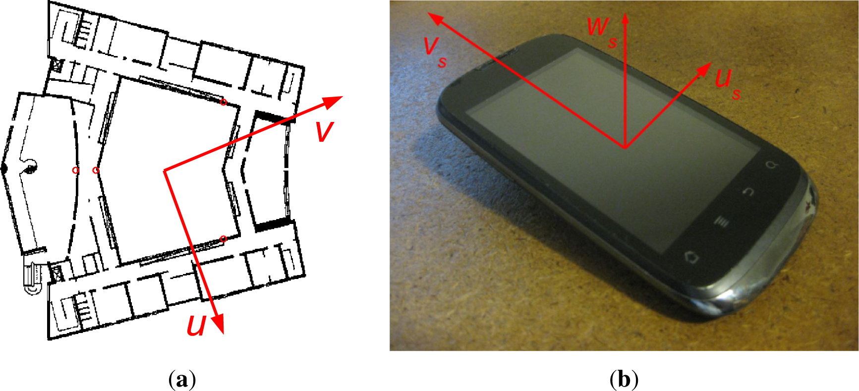
To be more specific, a minimal equipment of embedded sensors is required: a three-axis accelerometer, a three-axis magnetometer (e.g., MEMS-based inertial navigation system) and a Wi-Fi antenna. Furthermore, the navigation system is assumed to have access to the standard Wi-Fi network available inside the building. The installation of additional access points (APs) is not required (access points on one of floors of the considered building are shown as red circles in
Figure 1a).
In addition, to make the use of the system as simple as possible from the user’s point of view, no specific initial sensor calibration procedure is needed: the tracking algorithm that will be presented in Section 3 is designed to deal with uncalibrated sensors. Furthermore, as shown in Section 4, in order to improve the navigation performance, the system is designed to auto-calibrate the magnetic sensor during the navigation, e.g., exploiting regular user’s movements.
The rationale is that of using a dead reckoning-like approach [
8,
9]: detect the human steps by means of a proper analysis of the accelerometer measurements [
33], then use the combination of magnetometer and accelerometer measurements to estimate the movement direction with respect to the north [
28].
Since, in terrestrial applications, usually, the height with respect to the floor is of minor interest, then, hereafter, navigation is considered as a planar tracking problem (exceptions to this assumption are admitted, e.g., to deal with stairs and lifts). Let (
ut, vt) be the position of the device (e.g., smartphone), expressed with respect to the north and east directions (
i.e., global reference system;
Figure 1a shows the coordinate system in a university building used as the test field), before the
t-th step; then:
where
st is the length of the
t-th step and α
t is the corresponding heading direction. An estimation of the initial position (
u0, v0) is assumed to be (
a priori) available.
The step length
st is assumed to be provided by a proper analysis of the accelerator measurements [
33]. Alternatively,
st can be fixed to a constant value (an approximation of the mean step length): the tracking algorithm described in Section 3 is designed to compensate (relatively small) step length errors.
In most of the cases of common interest, the mobile device is supposed to be carried by the user’s hand (this is the case considered in the simulations of Section 5); however, the navigation system is expected to work in different conditions, as well. To be more specific, the system is expected to work as long as the heading direction is approximately fixed with respect to the local coordinate system (more details on this assumption are provided in the
Appendix) (
us, vs, ws) (the local coordinate system for a smartphone used in the simulations of Section 5 is shown in
Figure 1b). However, small deviations are allowed: the system of Section 3 is designed to estimate and correct heading direction discrepancies, with an absolute value lower than 36 degrees, with respect to the conventional direction.
Without loss of generalization, hereafter, the vs and the ws axes will be assumed to approximately correspond with the heading direction and with the vertical direction, respectively. Notice that these assumptions are not requirements of the proposed approach, but will ease the presentation of the method and the analysis of the calibration results shown in Section 5.
Notice that the update of
Equation (1) according to the sensor measurements provides an approximation of the device trajectory. However, it is well known that, because of measurement errors, the trajectory estimated by means of
Equation (1) quickly drifts from the correct one. In order to make the estimation method more robust, information provided by the dead reckoning-like approach has to be integrated with that provided by RSS measurements and the geometrical characteristics of the building (Section 3). RSS measurements of the standard Wi-Fi networks are provided by the corresponding antenna in the smartphone. The geometrical characteristics of the building are assumed to be pre-loaded on the navigation device or downloaded by means of the Wi-Fi network at the beginning of the navigation. As the mobile device gets inside of the building, it starts communicating with the Wi-Fi network, hence the device is considered as immediately ready to go (the total time for connecting the device to the network and to receive the information required by the navigation system depends on the specific conditions of the Wi-Fi network (e.g., signal strength, connection data rate, number of users connected to the network); however, the communication step is typically very fast (e.g., quantity of information to be passed < 100 kBytes in our simulations)).
Several nonlinear filtering strategies have been previously considered in the literature for the integration of information (e.g., INS and RSS measurements) in pedestrian indoor navigation [
8,
9,
16,
17]. Among such possible strategies, a particle filter approach [
19] is considered. In particular, our approach can be considered as a generalization of the particle filter proposed in [
17,
34], and that will be briefly summarized in the following (the reader is referred to [
17,
34] for a detailed description).
2.1. Widyawan et al. Particle Filter
Particle filter techniques are statistical methods widely used in complex (possibly nonlinear) estimation problems [
19–
24]. The variable of interest at time
t,
qt (e.g., the device position in the navigation problem considered here), is described by means of a density function
p(
qt|Yt), which depends on the values of the past measurements
Yt: the goal of the particle filter is to properly estimate such posterior density
p(
qt|Yt) (and update it when new measurements are available). Particle filters are particularly effective when dealing with complex systems, because of the two following characteristics:
The probability function p(qt|Yt) is not restricted to be Gaussian nor univariate; instead, it is described as the sum of a set of n particles.
No restriction is imposed on the dynamics of the system (i.e., it can deal with both linear and nonlinear systems).
However, when dealing with complex systems (e.g., nonlinear and with non-univariate density p(qt|Yt)), a large number of particles n has to be used in order to ensure good filtering performance: hence, the ability to deal with difficult scenarios is paid for with an increase of the computational complexity of the filter.
Several particle filter methods have been proposed in the literature, and each of them can be summarized as a specific algorithm used in order to properly updated the particle description of
p(
qt|Yt) when new measurements are available. The rest of this section is dedicated to the description of the particle filter for the indoor navigation proposed in [
17,
34], while a generalization of such an approach will be presented in Section 3 in order to efficiently deal with uncalibrated sensors (while keeping the number of particles
n relatively small).
Let
yt be the vector of measurements corresponding to the
t-th step and
Yt be the collection of measurements {
fτ} from τ = 0 to
t − 1. Furthermore, let
qt = [
ut vt]
⊤; then the probability distribution of estimated position
qt after the (
t − 1)-th step is expressed as follows:
where
qi,t and
wi,t are the position and the weight of the
i-th particle at
t, while δ(·) is the Dirac delta function.
In order to simplify the presentation, with a slight abuse of notation, hereafter, the subscript index t will be referred to as a time index, as well.
In this subsection, the INS sensor measurements are assumed to be unbiased, but affected by zero-mean random Gaussian noise, with heading direction and step length variance
and
, respectively. Then, the position of the
i-th particle at time
t + 1 is updated similarly to
Equation (1):
where
α i.t and
si,t are randomly sampled from the proper Gaussian distributions: α
i,t ~ N (α
t,
),
si,t ~ N (
st;). σ
α and σ
s are set to proper constant values (σ
α = π/2, σ
s = 0
:15 m in [
17]).
Exploiting an RSS channel model [
3], the RSS measurements are converted to distance measurements. Typically, the error on each measured distance is assumed to be normally distributed [
3,
17]. Then, the comparison of measured distances with the distances from the access points to the estimated device position yields the RSS probability
, that is the probability of being positioned in
given the RSS measurement in
yt (see [
3,
17] for details on
pRSS(·)).
Then, the particle weights are updated as follows:
Furthermore, particles with trajectories that violate the geometric constraints of the building are discarded. Then, the weights
are scaled in order to be normalized to one,
i.e.,
and the following distribution for the particles at time
t + 1 is obtained:
In the above equation, part of the particles may have very low weights (zero if the particle trajectory violates the building constraints); then, the effective number
of particles in
Equation (5) is typically lower than
n (a detailed study of the effective number of particles goes beyond the goal of this paper; for simplicity of exposition, hereafter,
at time
t will be considered as the number of particles, such that
wi,t is significantly greater than zero (
i.e., larger than a given threshold); the reader is referred to [
20,
21] for a more detailed description of particle filter characteristics). In order to preserve the effectiveness of the particle representation, the final approximation of the position distribution at time
t + 1 is obtained by resampling
n particles from
Equation (5),
i.e., the following actions has to be done for each resampled particle
i′: an index
i is randomly sampled accordingly to the probability
; then,
qi′;t+1 is sampled from a Gaussian distribution centered at
, and its weight is set to
wi′;t+1 = 1
/n (notice that the resampling step increases the estimation variance; see [
35] for a comparison of different resampling schemes).
The above approach can be summarized with the following procedure to be executed each time a new measurement is available:
For each particle
i:
- (1.a)
draw a sample
from the proposal distribution (
i.e., draw samples α
i,t and
si,t from
N (
αt,
) and
N (
st,
), respectively, then compute
with
Equation (3)).
- (1.b)
Set
= 0 if
violates building geometrical constraints; otherwise, set the weight
as in
Equation (4).
Scale the particle weights in order to normalize their sum to one:
.
Resample
n particles from
Equation (5) and set
wi′;t+1 = 1
/n, ∀
i′.
Notice that the number of operations to be executed for each particle in the above procedure can be upper bounded by a proper constant (and lower bounded, as well); hence, the computational complexity of the above particle filter is linear with respect to the number of particles n.
The reader is referred to [
17,
34] for details on the implementation of this particle filtering approach.
3. Tracking with Uncalibrated Sensors
The use of uncalibrated sensors can introduce temporally correlated measurement errors for both the heading direction and the step length. The following two subsections will separately consider these two cases, while Subsection 3.3 will summarize the overall approach.
3.1. Heading Direction Correction
The heading direction measurement
αt can be statistically described as follows:
where
is the correct heading direction,
αbs;t is an angular bias due to the use of an uncalibrated magnetometer,
αbe;t is an angular bias due to local perturbations of the terrestrial magnetic field typically due to the presence of ferromagnetic materials in the environment and
eα,t is a temporally random measurement error (that can typically be assumed to be white and Gaussian). The goal of this subsection is to approximately compensate for the bias
αb,t =
αbs,t +
αbe,t.
The following considerations are now in order:
When the device moves along a rectilinear trajectory, i.e.,
is (approximately) fixed to a constant value for t = ts,…,te, then αbs,t ≈ αbs,t′ for ts ≤ t ≤ te, ts ≤ t′ ≤ te.
Assuming the magnetic field to be sufficiently smooth in the considered environment, then locally αbe,t ≈ αbe,t′ for t ≈ t′.
Human trajectories are usually quite regular.
Then, the rationale is that of decomposing the device motion in piecewise (approximately) rectilinear trajectories. Each piece of such trajectories being approximately rectilinear and typically not so long, then:
for
t and
t′ in the same piece of (approximately) rectilinear trajectory.
The end of a piece of the (approximately rectilinear) trajectory (and consequently, the beginning of a new piece) is detected when the following condition holds:
where V indicates the logic operator “or” and
αthr is a proper threshold (
αthr = π/6 in the simulations of Section 5).
Accordingly to Condition
(8), the trajectory is divided in non-overlapping sections of (approximately) rectilinear trajectories. Let
ts,j and
te,j be the initial and ending time instant for the
j-th (approximately rectilinear) section. Then, in order to compensate for the bias
αb,t,
ts,j ≤
t ≤ te,j, Step 1.b of the particle filtering procedure presented in Subsection 2.1 is modified as follows:
- (1.b.1)
If
violates the geometrical constraints of the building, then resample
as follows: draw a rotation angle sample
from U(−αmax, αmax), and rotate
of an angle
around the vertical axis passing through
.
- (1.b.2)
Set
if
violates building geometrical constraints; otherwise, set the weight
as in
Equation (4).
Since the angular bias αb,t is approximately constant over an (approximately rectilinear) section of the trajectory ts,j ≤ t ≤ te,j, then Step 1.b.1 aims at compensating for such angular bias (if present), subtracting a randomly sampled angular bias
to the heading direction measurements over all of the trajectory section ts,j ≤ t ≤ te,j. Since no information about such an angular bias is available,
is randomly sampled from a uniform distribution in the interval (−αmax, αmax), i.e., U(−αmax, αmax), where αmax = π/5 in our simulations of Section 5.
Then, Step 1.b.2, which corresponds to Step 1.b in Subsection 2.1, has the task of properly filtering out particles associated with improper values of
(and of the other trajectory parameters).
3.2. Step Length Correction
The use of an uncalibrated accelerometer leads to a possible bias in the step length measurements:
, where st is the measured step length,
is the correct value of the step length, sb,t is the bias and es,t is a zero-mean white Gaussian noise with variance
.
In order to maximize the flexibility of the filter, but without excessively affecting the complexity of the filtering procedure, analogous to the previous Subsection, it is assumed that the value of the step length bias can be different in different sections of the trajectory; however, it is assumed (approximately) constant within each section (for simplicity of the filtering procedure, the same trajectory sections determined in Subsection 3.1 are considered here; nevertheless, the determination of a possible relation between the characteristics of human walking and of the step length bias will be the subject of a future investigation), i.e., sb,t ≈ sb,t′ for ts,j ≤ t ≤ te,j, ts,j ≤ t′ ≤ te,j.
Then, Step 1.a of Subsection 2.1 is modified as follows in order to take into account a possible step length bias:
- (1.a)
Draw a sample
from the proposal distribution: draw samples
αi,t and
si,t from
and
, respectively; then, compute
with
Equation (3)).
where, for each particle
i,
is randomly drawn from a uniform distribution
U(−
smax,
smax) at the beginning of each section of the trajectory.
is fixed to such a value for all of the time instants of the same section of the trajectory,
i.e.,
for
ts,j ≤
t ≤
te,j,
ts,j ≤
t′ ≤
te,j.
Then, as previously shown, Step 1.b.2 has the task of properly filtering out particles associated with improper values of
(and of the other trajectory parameters).
Finally, it is worth noticing that, when only INS measurements are available, the particle filter of Subsection 2.1 in open space results in being a biased estimator. For simplicity of exposition, assume that both heading direction and step length measurements are unbiased (or have already been properly compensated for). Furthermore, without loss of generality, it is assumed that
and that the device moves at time t from the origin of the global coordinate system, i.e., qt = [0 0]⊤.
Then, the following condition holds for an unbiased estimator:
where
ε[·] indicates the expectation operator.
Since the
αt distribution is symmetric with respect to zero, it is simple to show that
for a certain value of
s. In order to compute
s, consider the Taylor second order approximation of
ε[
s] for
αt =
eα,t ≈ 0 and
. Then,
Thus, for
, then
, and as previously claimed, the estimator is biased in open space.
However, in indoor navigation, it is also necessary to take into account the effect of the geometrical constraints of the building imposed in Step 1.b.2: the net effect of Step 1.b.2 is that of selecting those particles whose parameters are admissible with respect to the geometrical constraints of the building. Hence Step 1.b.2 leads the estimator towards the correction of its bias; however, this typically causes a decrease of the effective number of particles
, which is a working condition to be preferably avoided, if possible.
Motivated by the above considerations, the step length measurements can be scaled by a constant factor
k in order to compensate for the estimator bias:
Since, as mentioned above, the geometrical constraints of the building have a bias correction effect, from a practical point of view, it is possible to set
k to different values related to
Equation (12): for instance, in Section 5,
k is set to
.
3.3. Revised Particle Filter
The changes presented in the previous subsections with respect to the particle filter of Subsection 2.1 provide a revised particle filtering procedure that allows one to deal with uncalibrated sensors.
The overall particle filtering algorithm can be summarized as follows:
For each particle
i:
- (1.a′)
Draw a sample
from the proposal distribution: draw samples
αi,t and
si,t from
and
, respectively; then, compute
with
Equation (3).
- (1.b.1)
If
violates the geometrical constraints of the building, then resample
as follows: draw a rotation angle sample
from U(−αmax, αmax), and rotate
of an angle
around the vertical axis passing through
.
- (1.b.2)
Set
if
violates the building’s geometrical constraints; otherwise, set the weight
as in
Equation (4).
Scale the particle weights in order to normalize their sum to one:
.
Resample
n particles from
Equation (5) and set
wi′,t+1 = 1
/n.
Notice that, similarly to the original filter of Subsection 2.1, the computational complexity of the revised particle filter is linear with respect to the number of particles n. However, its computational burden is increased with respect to the original version (by 10%–20%, approximately, in the simulations of Section 5), mostly because of Step 1.b.1.
4. Auto-Calibration of the Magnetic Sensor
The algorithm presented in the previous section allows one to obtain good tracking results also in the presence of uncalibrated sensors (as shown in the simulations of Section 5). Nevertheless, the use of calibrated sensors, if possible, is obviously preferred. This motivates the presentation in this section of an auto-calibration procedure for the magnetic sensor.
The rationale is that of collecting magnetic sensor measurements during the regular use of the device (i.e., while the particle filter of Section 3 is running): compute the calibration of the magnetic sensor as soon as possible, and introduce the calibration model in the particle filter in order to improve its tracking ability.
Since the navigation problem has been considered as a 2D tracking problem and the heading direction has been assumed to be (approximately) fixed with respect to the local coordinate system, then the sensor calibration can be considered as a 2D calibration problem. To be more specific, since the heading direction and the vertical direction have been assumed to (approximately) correspond to the vs and ws axis, respectively, then the 2D calibration is performed on the (us, vs) plane, which (approximately) corresponds to the horizontal plane.
Despite the above assumption, it is worth noticing that in practical applications, the attitude of the device is typically not fixed to a constant value for all of the time instants: in practice, the attitude of the device will be assumed to be only approximately fixed, e.g., it oscillates around a mean orientation.
On the one hand, from the above considerations, it is clear that since the (us, vs) plane does not exactly correspond to the horizontal plane for all of the time instants, then even an extremely precise calibration of the magnetic sensor on such a plane cannot exactly compensate for the magnetometer error in all of the time instants. On the other hand, a complete (3D) calibration of the magnetic sensor requires a full set of rotations of the device, which actually should be avoided in order to simplify the use of the navigation system to the user. Thus, the aim of this section is just the computation of a rough calibration that allows one to reduce the magnetometer error (even if typically not completely compensating for it). The usefulness of this rough calibration will be shown in the results of Section 5.
The calibration procedure considered here is similar to that in [
26,
36,
37].
The following model for the magnetic sensor measurements is considered:
where
ym,t is the magnetic sensor measurement vector (projected on the (
us, vs) plane),
mt is the magnetic field orientation vector (projected on the horizontal plane and normalized to one),
em,t is the measurement error, while
D and
d contain the calibration parameters.
The goal of this section is that of estimating
D and
d from the measurements {
ym,t}
t=1,…,T, minimizing the sum of the squared norm of the errors:
The solution of the above optimization problem will be computed by means of an iterative procedure that will be presented in the following.
First, in order to initialize the iterative optimization procedure, an initial estimation of the parameter values is required.
Since
mt is a vector with norm one, then an initial estimation of the calibration parameters can be computed similarly to [
26]:
where
A =
D−⊤D−1,
b = −2
Ad,
c =
d⊤Ad − 1.
The equation
can be rewritten as a linear equation: Yθ ≈ 0, where θ = [vec(A)⊤ b⊤ c]⊤ (where vec(A) indicates the vectorized version of A (notice that A is a symmetric matrix; hence, only a set of independent parameters of A should be included in θ)), while Y is a matrix properly formed by the magnetic sensor measurements (at different time instants).
The equation
Yθ ≈ 0 can be solved (in least squares sense) by means of the singular value decomposition (SVD) [
38], yielding a solution vector ^ containing a scaled version
of the parameters in
A,
b,
c. The proper scale value
h can be computed as in [
26]:
.
Then, with a slight abuse of notation,
are redefined as follows:
.
The initial estimates
and
of the calibration parameters can be obtained as follows:
where the factorization of the
matrix (which can be computed for instance by means of the Cholesky factorization [
38] or with the SVD) is not unique. Indeed, let
be the matrix resulting from the Cholesky factorization of
; then, the factorization
holds, as well (for each rotation matrix
R).
Notice that, analogously to [
36], an estimate
of the rotation matrix
R can be obtained by solving an orthogonal Procrustes problem [
39]. However, such an estimate of
will not be necessary in the following.
Once initial estimates of the involved parameters are provided as above, then the following two steps are iteratively executed (until convergence) in order to compute the solution of
Equation (14):
Consider the values of
and
as fixed, and compute
, for t = 1, … T. Then, redefine
, for each t, by normalizing its norm to one:
.
Consider the values of
as fixed and compute
and
by minimizing:
Since, in this step, both
and {
ym,t}
t=1,…, T are considered as known, then the (least squares) solution of the above problem can be easily computed in matrix form, for instance, by means of the Moore–Penrose pseudo-inverse [
38].
Notice that, as usual, when dealing with iterative optimization techniques, the convergence of the proposed two-step procedure to the global minimum of
Equation (14) is not guaranteed.
The sensor model resulting from the magnetometer calibration procedure can be introduced in the particle filter presented in Section 3: when the calibration results are available, calibrated measurements are substituted to the {αt}, and Step 1.b.1 of the revised particle filter can be discarded (or can be executed, but setting αmax to a smaller value).
Since the use of a calibrated magnetometer can improve the performance of the particle filter, the calibration model should be used as soon as possible, i.e., as soon as it provides reliable results. The results of the calibration procedure presented above can be considered (roughly) reliable, provided that a minimal number of measurements (e.g., 20 in our simulations) are in all of the octants of the (us, vs) plane: once such conditions are achieved, the resulting calibration model can be used in the tracking procedure. Then, the calibration procedure shall be repeated later during the tracking of the device in order to reduce the calibration errors due to the possible small number of measurements in certain octants.
5. Experimental Validation and Discussion
The experimental validation of the method proposed in the previous sections has been assessed using a low-cost smartphone, Huawei Sonic U8650, in a building at the University of Padova. The considered smartphone is provided with a three-axis accelerometer (Bosh, BMA150, resolution 0.15 m/s2, maximum range ±39.24 m/s2), a three-axis magnetic field sensor (Asahi Kasei, AK8973, resolution 0.0625 μT, maximum range 2000 μT), and a Wi-Fi receiver 802.11 b/g/n. In the application used for the simulations presented in this Section, sensor measurements are acquired when changed values are detected by the system (e.g., by means of the Android sensor event method onSensorChanged); consequently, sensor data rates are not constant. In the simulations presented here, the approximate values of the average data rates are: 5 Hz for the accelerometer, 7 Hz for the magnetometer (since several magnetometer measurements are typically available for each human step, the heading direction is computed as the average angle obtained from such measurements) and 0.2 Hz for the Wi-Fi network (notice that such values are just indicative, because real sensor data rate values can be influenced by many factors).
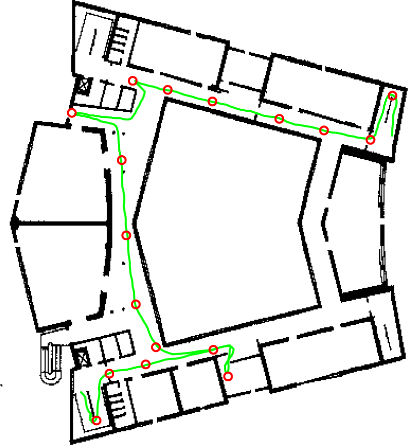
A set of 30 check points has been distributed along a track involving two floors of the building:
Figure 2 shows part of the trajectory (green solid line) and the check points positions (red circles) along the track. Other different tracks have been considered, as well: despite the numerical results being obviously slightly different, the performance trend is analogous to that presented here. In this sense, the case shown here can be considered as a general case (representative of the typical performance of the method).
In order to make the results independent of a specific stride, experimental data have been collected by three volunteers, two men and one woman, with heights from 1.65 m to 1.85 m, which completed the track with a number of steps ranging from 300 to 350. Actually, the results obtained by using the data collected by the three volunteers are quite similar: since no peculiarity has been found in the results of the tree datasets, the results presented in the following are obtained as mean values of those of the three cases.
Table 1 shows the positioning error results (root mean square error (RMSE)) obtained by using the device with uncalibrated sensors. More specifically,
Table 1 compares the results obtained with the proposed revised particle filter presented in Section 3 with those obtained with the particle filter of Subsection 2.1. The particle filter of Subsection 2.1 has been run with
n = 100 (in (a) and (d)),
n = 200 (in (b) and (e)) and
n = 500 (in (c) and (f)). Furthermore, two cases for the step lengths used in the particle filter have been considered: the length estimated by the sensor measurements (in (a), (b) and (c)), and the measured length corrected by the
k factor (in (d), (e) and (f)). The results shown in
Table 1 are the performance improvement (in percent) obtained by using the particle filter presented in Section 3 (with
n = 100) with respect to that of Subsection 2.1. Since the results obtained by means of the particle filter are non-deterministic (
i.e., they depend on the specific realization of the random noise used to run the filter), the reported results have been obtained by averaging the results of 100 independent Monte Carlo simulations.
The standard deviations σs and σα have been set to proper values accordingly to our simulations: σs = 0:15 m and σα = π/6.
Then,
Table 2 shows the results obtained on the same track considered in
Table 1, but using a (roughly) calibrated magnetic sensor. Calibration of the magnetic sensor has been performed as described in Section 4 by using 300 magnetic sensor sample measurements, {
ym,t}
t=1,…,300. The parameter values considered in
Table 2 are the same considered in
Table 1. Similarly to
Table 1, the reported results have been obtained by averaging the results of 100 independent Monte Carlo simulations.
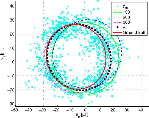
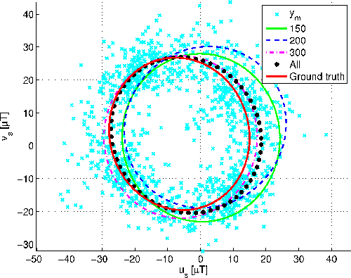
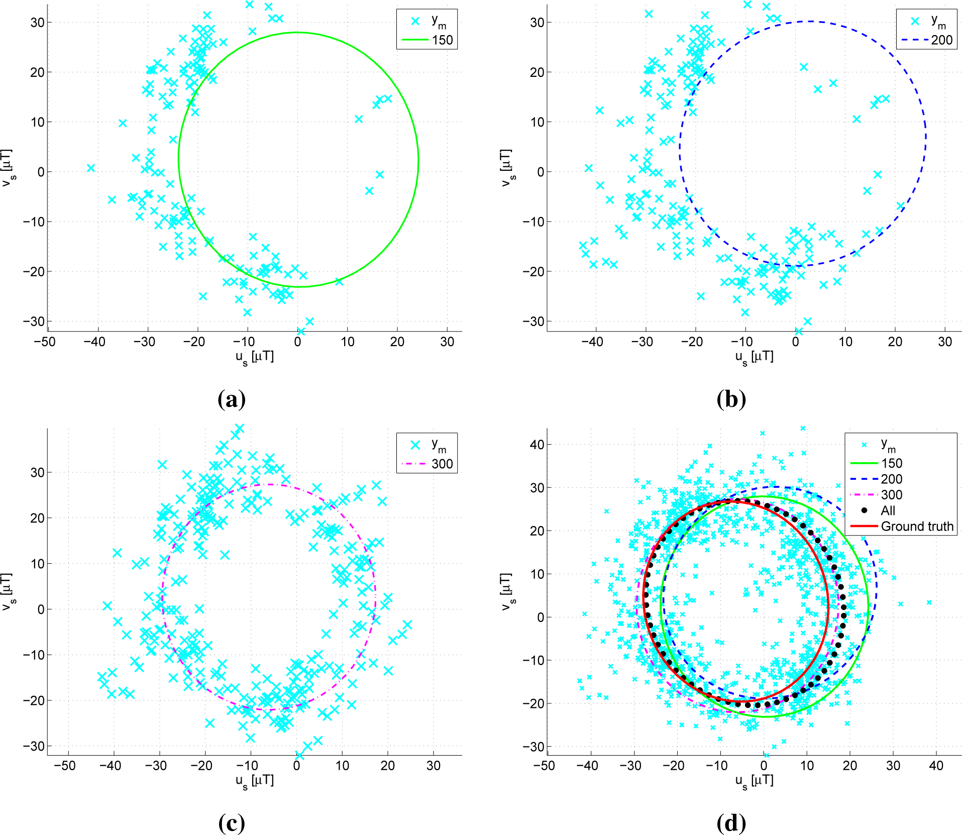
Figure 3 shows the magnetic sensor measurements and the corresponding fitting ellipse obtained with the calibration procedure described in Section 4. Calibration results are shown varying the number of sensor measurements used in the calibration process (sensor measurements are shown as cyan x-marks in
Figure 3): the results obtained with 150 (top-left, solid green line), 200 (top-right, dashed blue line) and 300 (bottom-left, magenta dashed–dotted line) measurements are compared in the bottom-right sub-figure with those obtained with 1000 measurements (black stars) and with the fitting ellipse obtained with a ground truth calibration (red solid bold line). The fitting ellipse in the ground truth calibration corresponds to that of the (
us; vs) plane, which, during the ground truth calibration process, was coincident with the horizontal plane.
Some considerations are now in order. First, notice that the results of
Table 2 have been obtained by using a roughly calibrated sensor,
i.e., calibrated by using 300 sensor measurements. As shown in
Figure 3 (bottom-right), 300 sensor measurements do not allow one to obtain a perfect calibration. However, since, in practice, the assumption of maintaining the (
us; vs) plane of a handhold device in an horizontal position can be only approximately satisfied, even with more measurements, the calibration results will typically differ from the ground truth ones: indeed, as shown in the bottom-right sub-figure of
Figure 3, the fitting ellipse obtained by means of 300 and 1000 measurements are quite similar, but they both differ from the ground truth fitting ellipse (red solid bold line).
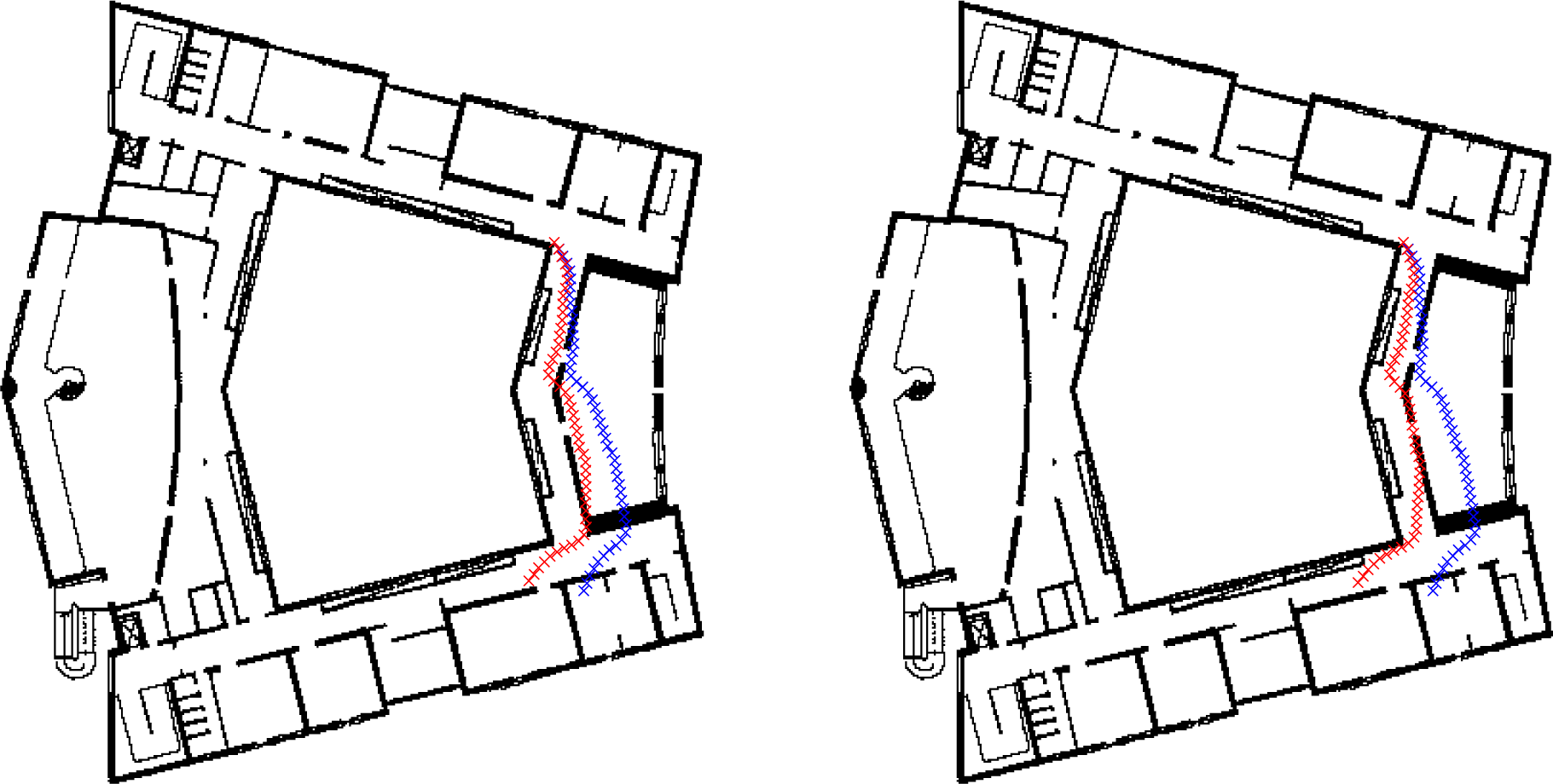
Nevertheless, actually, the use of a roughly calibrated magnetic sensor can allow one to improve the performance of the tracking system:
Figure 4 shows an example of unconstrained trajectories (
i.e., obtained by setting
αi;t =
αt,
si;t =
st and without imposing the building physical constraints), where it is possible to compare the results obtained by using the uncalibrated magnetic sensor (blue x-marks), the magnetic sensor calibrated with 300 measurements (red x-marks, left sub-figure) and the magnetic sensor with the ground truth calibration (red x-marks, right sub-figure). As shown in the figure, the trajectory obtained with the magnetic sensor calibrated with 300 measurements is quite similar to the one obtained with the ground truth calibrated sensor. Since the trajectories shown in
Figure 4 have been obtained by setting
αi;t =
αt,
si;t =
st, then they can be considered as (first) approximations of the average trajectories resulting from the particle filter (without imposing the building physical constraints) in the corresponding considered conditions: in this sense, the results shown in
Figure 4 can be considered as representative of the typical outcomes. This is confirmed by the results of our Monte Carlo simulations (
Tables 1 and
2), where the use of the proposed online calibration allows one to reduce by 30%, approximately, the estimation error of both the proposed algorithm and the original particle filter.
The results of
Tables 1 and
2 show that the use of step lengths corrected by the factor
k allows one to significantly reduce the tracking error of the particle filter. Furthermore, in all of the considered conditions, the revised particle filter proposed in Section 3 outperforms the other considered filtering approaches: despite being more clear in the uncalibrated case, its convenience is significant in the calibrated case, as well. This is probably due to the correction of local changes of the magnetic field (which yield local heading direction biases) that can be obtained by means of the proposed algorithm.
As expected, in the calibrated case, the improvement achieved by using the proposed algorithm decreases when n becomes larger; however, it is still significant even when the number of particles considered in the original particle filter (Subsection 2.1) becomes much larger than that of the revised particle filter of Section 3. In the uncalibrated case, since measurement errors are correlated, the original particle filter (Subsection 2.1) does not significantly improve increasing the number of particles from n = 100 to n = 500.
After the online calibration, the proposed algorithm achieves an average RMSE of (approximately) 3:5 m in the presented simulations by using n = 100 particles. Such performance is expected to improve by increasing the number of particles. However, considering that a larger number of n would significantly increase the computational load of the algorithm, which, according to our simulations, is approximately 10%–20% larger than in the particle filter of Subsection 2.1 with the same number of particles, n = 100 (however, notice that the computational load changes at each run of the algorithm, e.g., depending on the number of violated constraints).
According to the results obtained in the considered simulations, the particle filter approach proposed in Section 3 allows one to significantly improve the positioning results obtained with the filter of Subsection 2.1 in the case of uncalibrated embedded sensors and mobile device carried by the user’s hand (notice that in [
17,
34], the use of the particle filter described in Subsection 2.1 was proposed for a different system, where sensors where integrated in the user’s shoe). Such performance improvement has been obtained with a relatively small increase of the computational burden of the filter. Better results can be obtained by considering a larger number of particles
n; however, issues with the real-time implementation of the system will arise for
, with
sufficiently large. The actual value of
depends on the computational capabilities of the considered device (
n ≈ 100 particles can be used for real-time applications in standard mobile phones).
Notice also that despite the proposed approach allowing the use of a mobile device carried by the user’s hand, the obtained results might be improved by imposing more restrictions on the system (e.g., fixing the device to the user body, for instance to the shoe, as in [
17]), or by integrating other sensors (e.g., the integration of camera measurements has been considered in [
14]). Furthermore, the considered approach allows a partial, but not complete, freedom of movement to the user’s hand.
Motivated by the above considerations, our future works will aim to improve the proposed method, while preserving the use of a relatively small number of particles:
The presented approach considers two different working conditions (i.e., before and after the magnetic sensor calibration results are available). However, even if the magnetometer calibration results are not yet available, the data collected can be used to improve the algorithm presented in Section 3, e.g., in Section 3, the guessed bias angles
and
are chosen independently; instead, it is clear that they are (partially) related accordingly to the sensor model: the selection of the bias angle
should be done accordingly to the data already collected.
An extension of the proposed approach should be considered in order to let the heading direction freely vary with respect to the local coordinate system.
Finally, the presented navigation algorithm will be integrated in a mobile mapping system in order to provide accurate 3D photogrammetric reconstructions of the environment ([
40–
45]) based on the use of the camera embedded in the mobile device.


