Effect of Tariff Policy and Battery Degradation on Optimal Energy Storage

Instituto de Ingeniería Química, Facultad de Ingeniería, Universidad de la República, Montevideo 11300, Uruguay
*
Author to whom correspondence should be addressed.
Processes 2018, 6(10), 204; https://0-doi-org.brum.beds.ac.uk/10.3390/pr6100204
Submission received: 15 September 2018
/
Revised: 19 October 2018
/
Accepted: 19 October 2018
/
Published: 22 October 2018
(This article belongs to the Special Issue Modeling and Simulation of Energy Systems)
Abstract
:In the context of an increasing participation of renewable energy in the electricity market, demand response is a strategy promoted by electricity companies to balance the non-programmable supply of electricity with its usage. Through the use of differential electricity prices, a switch in energy consumption patterns is stimulated. In recent years, energy self-storage in batteries has been proposed as a way to take advantage of differential prices without a major disruption in daily routines. Although a promising solution, charge and discharge cycles also degrade batteries, thus expected savings in the energy bill may actually be non-existent if these savings are counterbalanced by the capacity lost by the battery. In this work a convex optimization problem that finds the operating schedule for a battery and includes the effects of current-induced degradation is presented. The goal is to have a tool that facilitates for a consumer the evaluation of the convenience of installing a battery-based energy storage system under different but given assumptions of electricity and battery prices. The problem is solved assuming operation of a commercial Li-ion under two very different yet representative electricity pricing policies.
1. Introduction
Connecting renewable energy sources to the electric grid changes the classical paradigm: as these sources are non-programmable an imbalance between electricity generation and electricity consumption is created. As electricity as such cannot be stored, two main strategies have been proposed to overcome the imbalance: conversion of electricity to a type of energy that can be stored and demand response [1,2]. In the former, energy storage, the amount of electricity that is produced in excess at a certain time is centrally converted to for example potential energy (through mechanical pumping) or chemical-electrochemical energy (e.g., production of or large-scale batteries). Then, when needed at a later time, this energy is reconverted to electricity and discharged to the grid. In the latter, demand response, a change in electricity consumption habits to match the production rate is sought. This change in habits is promoted by adjusting the price of electricity at different times: when there is an expected large demand or low production of electricity, its price increases, and the opposite when demand is low and supply is large. The term tariff policy or pricing policy refers to the electricity price schedule that companies develop to stimulate demand response. In this context, many energy markets have developed different tariff policies [3,4]. Broadly speaking, tariff policies can be classified as pre-established and on-spot. On on-spot tariffs, electricity prices and even allowed amounts of energy that might be purchased, are announced publicly shortly before the expected consumption (from minutes, up to one day ahead). On pre-established tariffs, electricity prices are known to consumers, but might be different for weekdays and weekends/holidays, and, within each day, they might change hourly. These types of tariffs are also known as time of use pricing (TOU).
Implementation of these policies have given the consumers the opportunity of reducing the total cost of the electricity they use, by increasing their energy consumption when electricity price is low and reducing the consumption when the price is high. Still, not all uses can be managed this way. In particular, in the residential sector, major savings imply a large reorganization of daily routines, which is only worth if there is a strong penalization in the hours that energy consumption is to be reduced. For residents or small-scale businesses, self-storage represents a more suitable non-routine disruptive way to achieve savings in electricity costs. For these purposes, electrochemical, thermal, and even an increase in inventory when the price is low, have been pointed out as valid self-storage alternatives [5].
Along these lines, how to optimally store energy to maximize savings is a problem currently being addressed in the literature, a complete review can be found in Weitzel and Glock [6]. With the foreseen decline in the costs of batteries [7,8] incorporation of this kind of energy storage solution may soon be economically viable for all sectors, including small enterprises and households. This economic viability will depend on both the savings due to TOU and battery lifespan and replacement cost.
Battery lifespan and replacement cost depend on its degradation rate, which in turn depend on how much and how the battery is used. The relevance of including these factors when formulating problems to find an optimal battery operation policy has been recognized in Reniers et al. [9]. Battery degradation mechanisms depend on many factors, in particular, the rate of charge/discharge has a large effect. As in all electrochemical devices, charge/discharge due to electrochemical reaction, and current density are related by Faraday’s Law. Larger currents result in shorter charge/discharge periods; however, as electric current increases, so does the overpotentials, which may favor secondary effects. These effects contribute to capacity loss in batteries during operation [10,11].
The goal of this paper is to formulate an optimization problem for finding the optimal operation schedule for a battery that also includes current-induced battery degradation. Other contributions have also considered battery degradation in the formulation of their optimization problems: Sarker et al. [12] showed that not taking into account battery degradation results in a solution that leads to an operating schedule that actually depletes the battery faster than the solution that is found when considering these effects directly in the optimization problem; Yan et al. [13] showed a similar effect but with a slightly different use: that of the battery being used as a frequency regulator; Hu et al. [14] considered the cost of battery degradation in energy management of plug-in hybrid electric vehicles.
Unlike a previous mixed integer linear problem (MILP) [12], in this paper a convex formulation is presented. The advantage of this formulation lies in the fact that global optimality is guaranteed, and also that with the same computing capabilities, problems considering longer time spans (not only a single day) can be solved. This in turn allows the estimation of the leftover capacity of the battery after a certain number of cycles. This is precisely the main novelty of this paper: the capability of predicting the effects that different pricing policies have in long-term optimal operation scheduling, when battery degradation is taken into account.
In all case studies Li-ion batteries, an energy storage device that presents an outstanding specific energy and power, long calendar and cycle lives, high efficiency and reliability [15], were considered. The paper is organized as follows: Section 2 presents the basic optimization problem and its convex form; using this model, the optimal daily operation for two different pricing policies (simple and complex) are presented in Section 3. An extension to the model in Section 2 that captures the cumulative effect of battery usage is presented in Section 4.1. Section 4.2 and Section 4.3 present the long-term optimal operation schedule for the same tariffs considered in Section 3. Finally, the key points of the paper are summarized in Section 5.
2. Problem Statement and Model Formulation
2.1. Objective Function
Throughout the paper we will consider a consumer who wants to install a Li-ion battery as a way to take advantage of a given pre-established TOU tariff policy. We will assume that the consumer has already chosen the capacity that needs to be installed and the general problem is how to optimally operate the battery so that savings in the electricity bill are larger than the costs induced by its use. Then, the objective function from the user point of view can be expressed as:
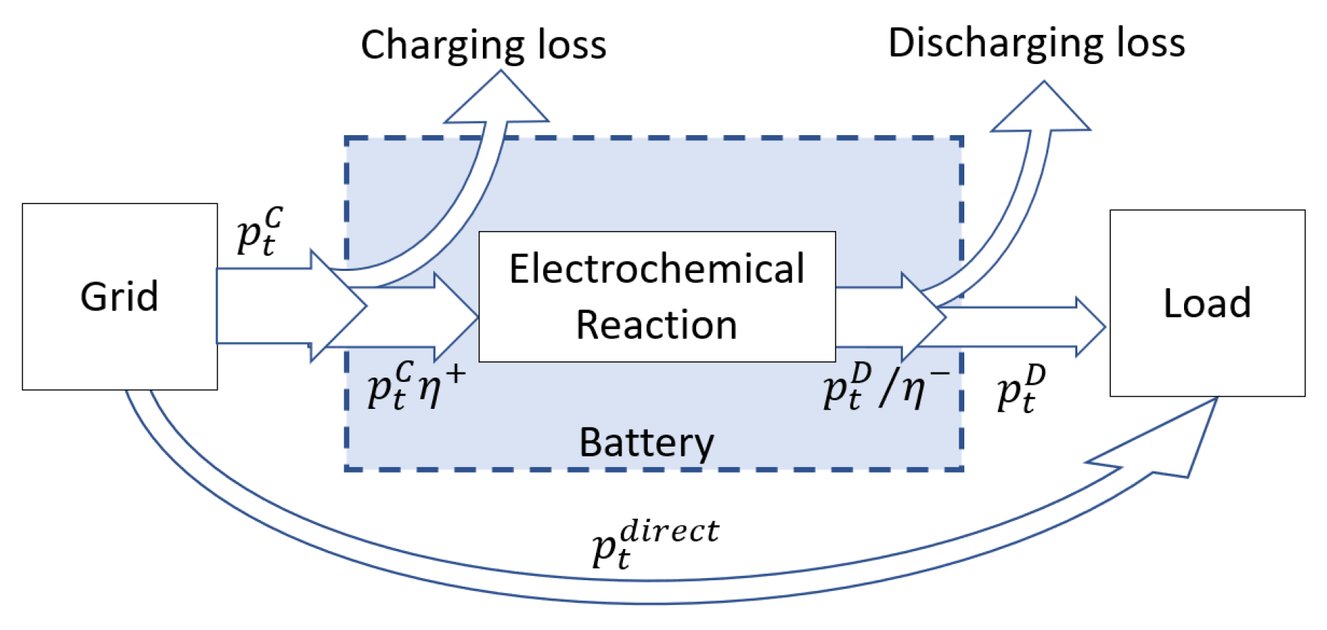
As shown in Figure 1, when being charged, at a moment t, the battery takes energy from the grid at charging power ; when being discharged, at a later time , the battery feeds a load (for example a house) at discharging power . Besides, the energy that the battery receives from the grid and the energy the load receives from the battery are affected by efficiency factors denoted as and respectively. At times, it might be more convenient to by-pass the battery and feed the load directly from the grid. This is shown in Figure 1 as the direct power flow .
Using these variables the savings in electricity can be expressed as:
where and denote the price of the electricity at different times as given in the tariff policy.
On the other hand, the cost of capacity loss due to operation can be written as:
where denotes the cost of the technology in USD/kWh; is the installed capacity, a fixed parameter with units kWh; and is the fraction of capacity lost during operation time . Note that is a dummy variable: during charge and during discharge.
Then, for a given period of time divided into smaller time steps , with equal to the minimum electricity pricing step, the objective function can be stated in canonical form as:
2.2. Constraints
In Equation (6) the terms , , are parameters, whereas the terms , and are decision variables of the problem. These variables are related to each other and to other decision variables through the following constraints:
- The battery cannot charge and discharge at the same timeThis restriction can be mathematically posted as
- For safety reasons, there is a maximum power that should not be exceeded neither during charge () nor during discharge (). Additionally, and will always be assumed as positive variables. Then:
- Energy balance: the state of charge at a certain time, , depends on the state of charge at the immediately previous period of time and the amount of energy that is effectively used in electrochemical reactions during charge or discharge processes:where the efficiencies are as defined previously (see Figure 1).
- In order to preserve the battery life, the state of charge should neither be lower than a minimum fixed value () nor larger than a maximum (). Both these parameters correspond to different fractions of the total available capacity.
- Equations for battery degradation:Battery degradation kinetics are studied in the electrochemistry field by using a parameter known as the [16,17]. The is the inverse of the characteristic time that relates electric current during a time step, in units of A or mA, and the electrical charge capacity of the battery, in units of Ah or mAh.This coefficient allows a size-independent study of the kinetics of any reaction happening in batteries. The fraction of capacity lost by the battery can then be expressed as a function of the .where the functionality f is obtained experimentally by running charge/discharge cycles at different currents, and is usually a non-linear expression. Taking as a basis the experimental data reproduced in Figure S1, it can be seen that can be modeled as a convex second order polynomial.with and parameters that are adjusted to the experimental data.To relate the from its definition (Equation (12)) with the variables used in this problem, a nearly constant working potential of the cell needs to be assumed. In practice, this assumption implies disregarding the effects of the overpotentials in the potential vs. current (E-I) curve. Then, and:Notice that as charge and discharge do not happen simultaneously (see Equations (7) and (15)) can be rewritten to combine both processes in a single equation:At this point, it is worth commenting that natural aging phenomena (just a function of time) has not been considered here as calendar aging is not dependent on the rate of battery use.
Therefore, given the objective function (Equation (6)) and the restrictions (7)–(11), (14), (16) the problem is a non-linear programming (NLP) problem where the decision variables are ,,, and . As stated, the problem has two non-linear equality constraints (Equations (7) and (14)) thus it is non-convex. Relaxations, that result in an equivalent convex problem are discussed in the following section.
2.3. Derivation of an Equivalent Convex Problem
2.3.1. Non-Simultaneous Charge and Discharge
Equation (7) is the equation that states that simultaneous charge and discharge processes are not possible. Besides the product-based formulation used here, a formulation employing a binary variable that multiplies either or has been reported in Jabr et al. [18]. However, this approach leads to a mixed integer problem (MILP or MINLP) which does not solve the fundamental convexity problem.
In this work we will make use of a result in Castillo and Gayme [19].
“For energy storage capacity at bus where (the energy storage capacity) , if (the locational marginal price) is strictly positive then (...) simultaneous charging and discharging will not occur”.
This result was obtained in the context of optimal allocation and operation of a distributed energy storage system, in a network of generators, storage devices and consumers, where the price of the energy was not included as a parameter of the model, instead it was estimated through the dual variable which is referred in the paper as a market-based price signal.
Despite our overall problem formulation is different, from the energy storage device, i.e., the battery, the situation is similar as in both cases the energy storage device consumes from an upstream energy provider and supplies to a downstream load. In our case the electricity prices are given and correspond to the TOU tariffs which are always positive. Then, it is reasonable to assume that the result from Castillo and Gayme [19] will also be valid here, and and will not be non-zero at the same time. At a more fundamental level, the explanation is that as charge/discharge efficiencies are always lower than 1, simultaneous charge and discharge just dissipates energy. Hence a portion of the energy consumed does not result in an effective change in the state of charge of the energy storage device, an effect that is usually not sought.
Therefore, based on the above discussion, Equation (7) will be excluded from the formulation of the problem; upon finding the optimal solution in different case studies a check will be performed in order to assess the validity of the relaxation.
2.3.2. Battery Degradation
Equation (13) is the equation relating the fraction of capacity lost by the battery for different . As discussed previously, this equation is derived by fitting experimental data and results in a convex expression as the parameter is positive. As in Equation (6) the variable is multiplied by positive values, an increase in the value of will directly imply an increase in the objective function. Hence, if the equality constraint in Equation (13) is relaxed to the convex inequality constraint in Equation (17):
minimization of the objective function will always result in an active constraint, thus the same optimal solution.
At this point it should be noted that although we started from a particular case (experimental data for Samsung INR 18650 reported in Sarker et al. [12]) it has been experimentally observed that other types of batteries also present a convex functionality between the capacity leftover in the battery after a certain number of charge/discharge cycles () and the [20]. Thus, the relaxation presented here can be generalized if other batteries, with other convex functionalities, are considered. Despite the details are not yet clearly understood, the convex functionality is to be expected as increasing the current increases the overpotentials. Thus both, the number of undesired events (physical or chemical) and the rate at which these events happen increase creating a snowball effect in terms of battery degradation [11,21,22].
2.3.3. Problem Statement in Convex Form
Following the discussion in the previous section, we present here the canonical form of the convex NLP problem which is equivalent to the one discussed in Section 2.2.
The problem is implemented in GAMS 24.8.5 and solved with IPOPT [23].
3. Optimal Scheduling for a 24 h Period
In this section, the optimal charge/discharge schedules for different tariff policies are presented. The simulations were run considering an example of each of the two most extreme TOU pricing policies:
- The “simple tariff” refers to a pricing policy that only has two price steps: cheap (off-peak) and expensive (on-peak), and the daily price pattern is repeated throughout the year. Therefore, there are always some consecutive hours with exactly the same price.
- The “complex tariff” refers to a pricing policy where there are several price steps during a single day (the price is still constant for each hour of the day), different days present different prices (weekdays are priced differently than weekends and holidays and there is also seasonal variation), and prices are dependent on the expected weather.
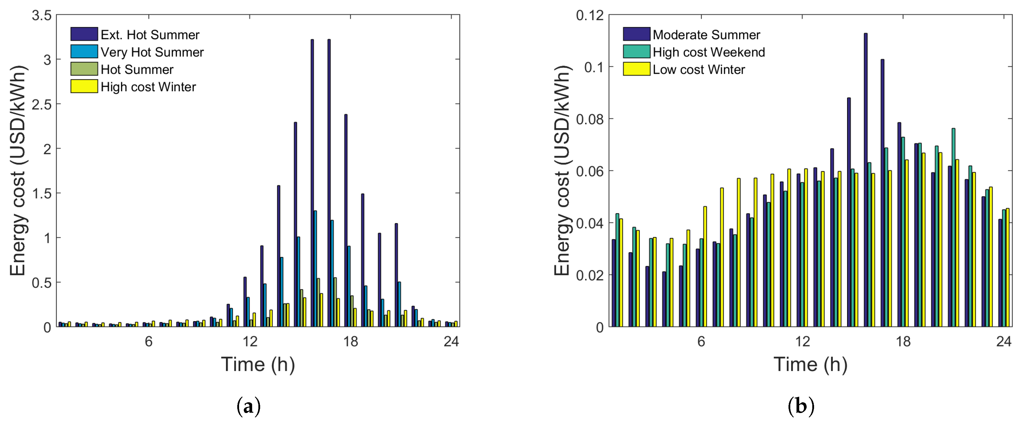
An example of a “simple tariff” is given by the Uruguayan residential “UTE-Tarifa Inteligente” (smart rate) which consists of an 18 h period at a cheap rate, and a 6 h period at an expensive rate [24]. An example of a “complex tariff” is given by the Californian Southern California Edison tariff [25]. For medium consumers, this tariff classifies days into nine groups according to: High and Low cost Weekend; Extremely Hot, Very Hot, Hot, Moderate and Mild Summer Weekday, High and Low cost Winter Weekday. Both for winter and weekends classes, “High cost” and “Low cost” depend on the expected temperature.
Other TOU tariffs are in between the previous two extremes. For example the Brazilian “Tarifa Branca” [26], is a three-step simple tariff with the: cheap-medium priced-expensive-medium priced-cheap pattern on weekdays and cheap pattern on weekends. Another example is Iowa’s residential hourly pricing option [27] which is a two-step tariff which also differentiates between winter and summer.
In all cases, the maximum is assumed to be 3; then maximum power and capacity ratio are related as . Upper and lower bounds for the state of charge () are assumed to be 80% and 20% of the installed capacity respectively. Both and are assumed to be 0.95 and installed capacity is set at 10 kWh. Furthermore, we will assume that the battery is initially discharged (i.e., ). The coefficients for the battery degradation equation are = 1.06 × 10⁻⁵ and = 1.44 × 10⁻⁴ (see S1 in Supplementary Information). Estimated 2018 battery prices range from 580–750 USD/kWh for commercial and residential use [28]. However, as Li-ion battery systems still have margin to lower their production costs [29], battery prices used in the simulations were selected case by case to show key features of each case study.
3.1. Results and Discussion: Simple tariff
Figure 2a shows the TOU tariff used in Uruguay: electricity is cheap between 0:00 a.m.–5:00 p.m., significantly more expensive between 5:00–11:00 p.m., and cheap again during the last hour of the day (11:00 p.m.–0:00 a.m.). Note that in Figure 2a we have redefined the time vector so that all low prices are together. In practice, this change means that a “storage day” starts at 11:00 p.m., and allows the one-day simulation to exploit the whole off-peak price period.
The optimal results for , , and for three different battery prices () are shown in Figure 2b–d.
Notice that for a battery price of 500 USD/kWh the optimal solution neither takes power from the network nor supplies power to the load, and the battery remains constant at the initial level. The reason is that in this case, the economical penalty for degrading the battery is larger than the savings for taking advantage of the TOU tariff, thus the battery should not be installed.
For battery prices of 300 and 400 USD/kWh, the optimal strategy is to slowly charge the battery during the whole low-price period at a steady rate, and then discharge it as slowly as possible during the high price period. This strategy results in low for both charge and discharge thus low degradation factors . The strategy itself is the same for both battery prices, then total savings in the energy bill are the same (0.86 USD/d). However, as the penalty due to loss of battery capacity depends on initial battery price, overall savings are different and lower than bill savings: 0.34 USD/d and 0.17 USD/d for the 300 USD/kWh and 400 USD/kWh respectively.
and are never simultaneously non-zero and, as shown in Supplementary Materials, the value of the Kuhn-Tucker multipliers verifies that Equation (21) is always active. Thus, the assumptions made for convexification of the problem are checked.
3.2. Results and Discussion: Complex Tariff
Figure 3 shows the TOU tariff used by Southern California Edison Company (TOU-GS-2-RTP); days presenting a large variation in the tariff are shown in Figure 3a, whereas days with moderate variations are shown in Figure 3b.
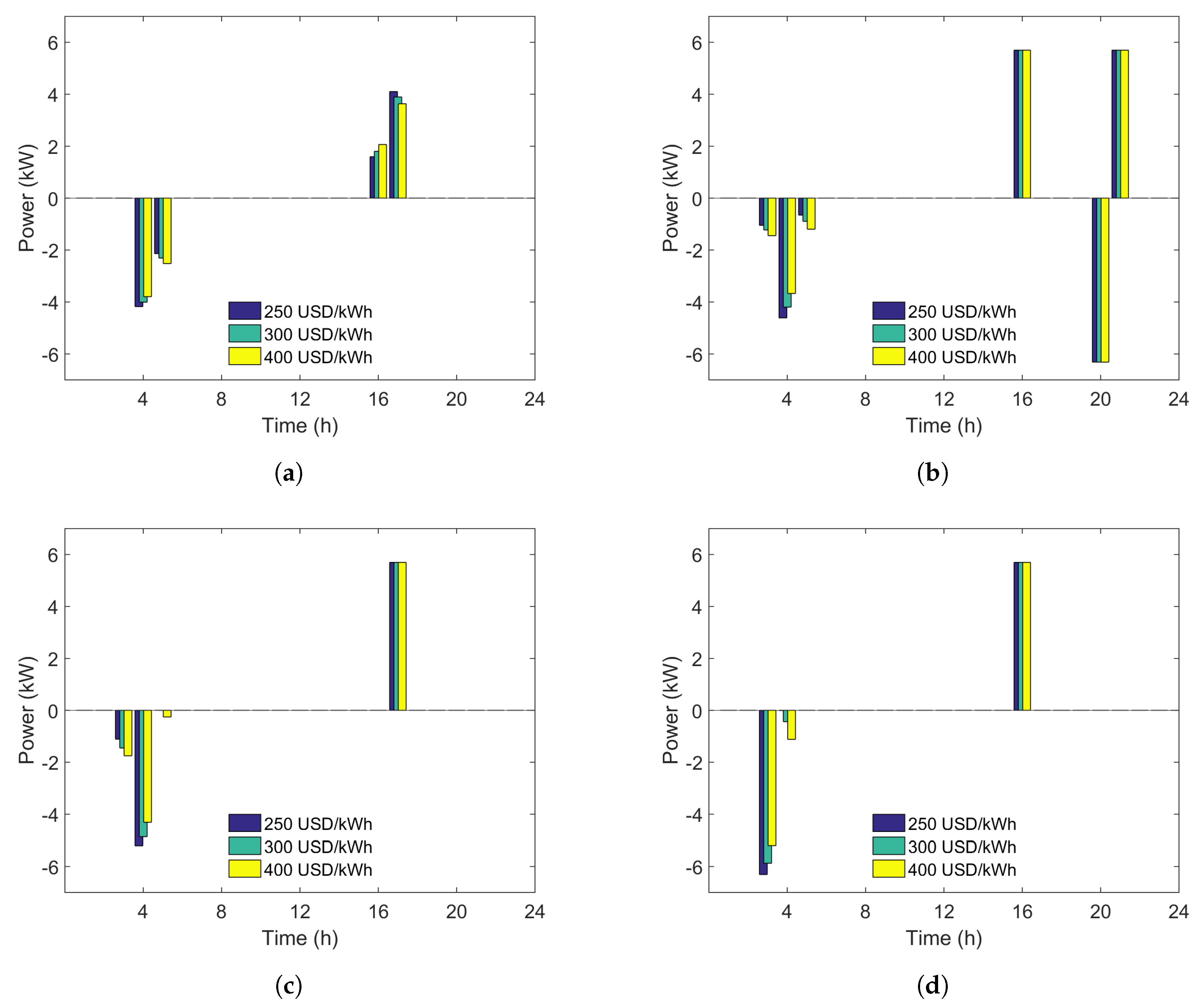
In this case there are in principle 9 different optimal strategies each corresponding to a different day-type as discussed at the beginning of the section. However, from these nine price schedules, only four result in a non-trivial operation for batteries that cost 300 USD/kWh. The four price schedules that result in non-trivial operation coincide with the ones that have the largest variation between the maximum and the minimum electricity prices (i.e., Figure 3a). Figure 4 shows the optimal charge/discharge schedule for battery prices of 250, 300 and 400 USD/kWh. As the battery price decreases, moderate-priced days start also to show non-trivial operation, see as an example Figure S4.
Compared to the first case study the most noticeable difference is that charge and discharge are now concentrated and not distributed during the day. For example, for Extremely Hot Summer Days (EHSD) charge is concentrated in two hours (3:00–5:00 a.m.) and discharge is concentrated between 3:00–5:00 p.m. (see Figure 4a). Notice also that unlike the “simple” tariff the rate of charge/discharge varies. This effect is seen in Figure 4a in the EHSD case: between 3:00–4:00 a.m. the battery consumes more power than between 4:00–5:00 a.m. Logically this is related to the price of the energy during those hours. In absolute terms, for the days that operation is allowed, this “complex” tariff results in a faster degradation of the battery than the “simple” tariff considered before. Figures with degradation rates are in the Supplementary Information (S3).
The difference in pricing also allows for some days to have a double charge/discharge cycle. For example, for a Very Hot Summer Day (VHSD) the first charge is between 2:00–5:00 a.m., the first discharge is between 3:00–4:00 p.m., the second charge is between 7:00–8:00 p.m. and the second discharge is between 8:00–9:00 p.m. This double cycle is allowed by the relatively large difference between the prices corresponding to the 7:00–8:00 p.m. and 8:00–9:00 p.m. interval.
Another salient feature of the complex tariff is that a difference in the cost of the battery affects the optimal operation: although the time of the day at which charge/discharge occurs is the same, the amount charged within each interval is different.
As in the previous case, all assumptions for problem relaxation were satisfied.
4. Optimal Scheduling for Long-Term Periods
4.1. Modifications to the Original Problem
4.1.1. Variable Capacity
In the previous sections we showed how the optimal operation schedule was affected by the TOU tariff and the cost of the storage system itself. In this section, we expand those results to a more realistic setting in which the battery is going to be used during several years. As longer optimization periods are considered, charge and discharge cycles may result in a significant loss of capacity, and the problem presented in Section 2.3.3 needs to be modified in order to allow for a daily change in the capacity of the battery. In other words, capacity is now a variable which will be represented by .
Without loss of generality we will consider daily changes in (i.e., ) and not hourly changes, a consideration that is supported by the small hourly values obtained for in Section 3. However, as the tariffs still vary on an hourly basis, two time scales need to be considered: day and hour. As a result the variables in the previous sections will now be represented using both time scales (, , , ).
As changes daily so do the allowed upper and lower bounds of the state of charge. Then, and . If we still keep the same criteria (state of charge between 20% and 80% of the remaining capacity), then Equation (22) should be replaced by Equation (25):
Also, as changes, the maximum power at which the battery can be charged or discharged safely, varies. Keeping the same limit as in Section 3 () then Equations (26) and (27), substitute Equations (23) and (24).
4.1.2. Restricted Time Span between Charge and Discharge Periods
Complex tariff systems that present large differences between the highest and the lowest prices may provide an optimal schedule in which the battery charges months before it discharges. This strategy, even when acceptable, it is not practical as:
- If energy is stored in batteries for a long period of time, self-discharge processes occur. For the sake of simplicity our model has not included these types of processes under the assumption that the charge and discharge cycle of the battery happens in a reasonably short period, most probably during the same day.
- Complex tariffs depend on weather conditions and thus a reliable forecast. In this work we have assumed that reasonable forecasts are given for periods no longer than a week.
Then, to restrict the length between charge and discharge periods, Equation (28) was included as an extra restriction to the long-term optimization problem:
As written, Equation (28) indicates that the net power consumed by the battery at a certain time must be lower than the sum of the power supplied from the battery to the load during the following week (). Depending on the technology used, this restriction could be tightened by using a smaller .
4.2. Results and Discussion: Simple Tariff
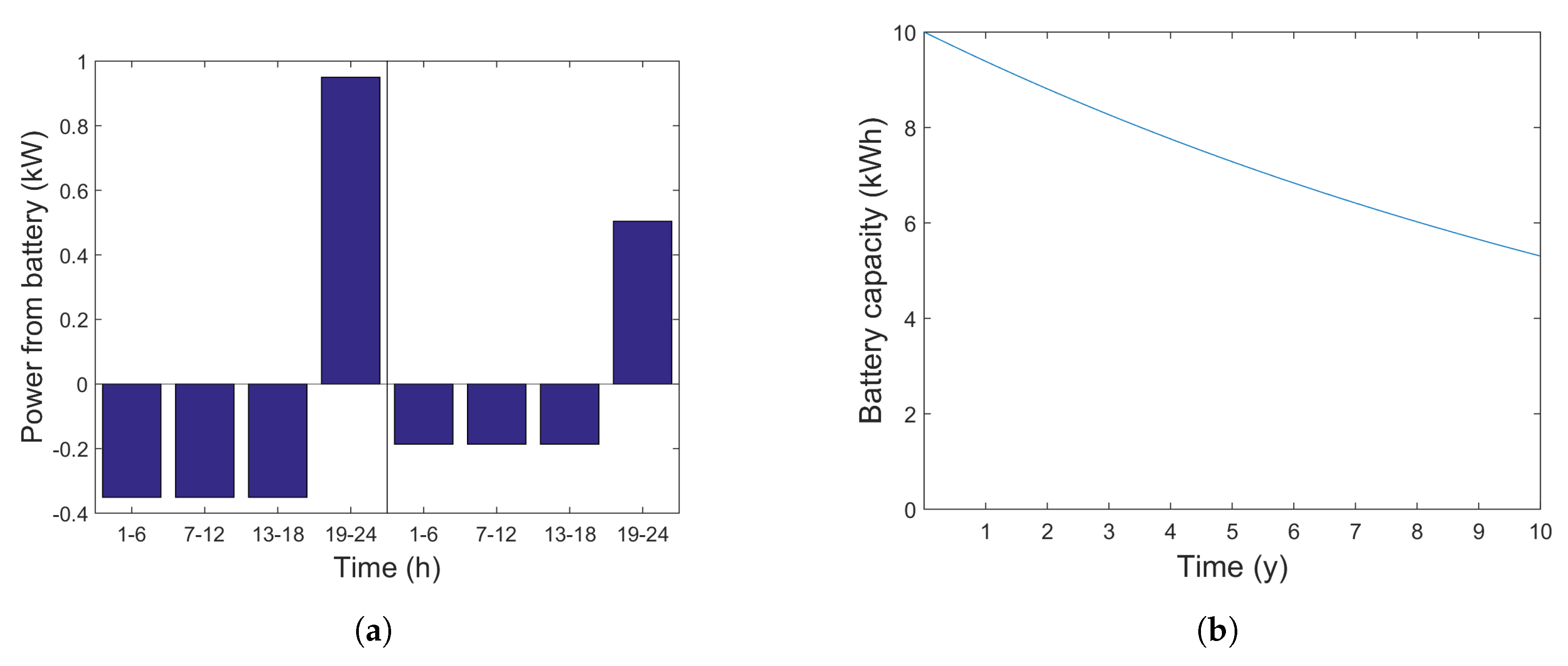
Figure 5a shows the charge/discharge strategy ( and ) for the battery for the first and last days of use. As the tariff has two steps and remains constant for all days, the operation policy is the same as in the one-day case: slowly charge and discharge. The difference between the first and last day is the rate at which power is consumed/supplied, which diminishes with time due to battery degradation.
The capacity remaining in the battery at each time is shown in Figure 5b. As seen after 10 years the battery still retains 53% of its original capacity.
As in the case discussed in Section 3.1, for a non-trivial optimal, the price of the battery affects the value of the objective function, but not the value of the variables , , , . Table 1 shows the yearly savings in electricity bills for capital costs below 400 USD/kWh (i.e., a price that guarantees a non-trivial solution). The net savings considering battery degradation over the operation period are 922 USD and 453 USD, for the 300 USD/kWh battery and 400 USD/kWh battery, respectively. The net present values calculated as:
are presented in Table 2 for different battery prices and rates (r). Roughly, prices below 140 USD/kWh are required for batteries to be economically viable. This value is in agreement with the 125 USD/kWh target established by the DOE for battery prices for electric vehicles [7].
4.3. Results and Discussion: Complex Tariff
Figure 6 shows the maximum temperatures recorded in Los Angeles, CA, during each day of 2017 [30]. As mentioned earlier, maximum temperature is the key parameter to establish the electricity price in the example of complex tariff used in this paper. The temperatures themselves are represented with bullets, whereas the colored blocks represent the tariff that would be applied for each day according to season and temperature effects (for clarity values for weekends were omitted in the graph). The full line in the graph represents the historical average for maximum temperature. Note that using averages is not suitable for running the simulations as no day would be classified in the extreme temperatures, which, as discussed in Section 3.2, are precisely the days that provide a non-trivial optimal solution. For this reason, all simulations in this part of the paper where run assuming the temperatures recorded in 2017.
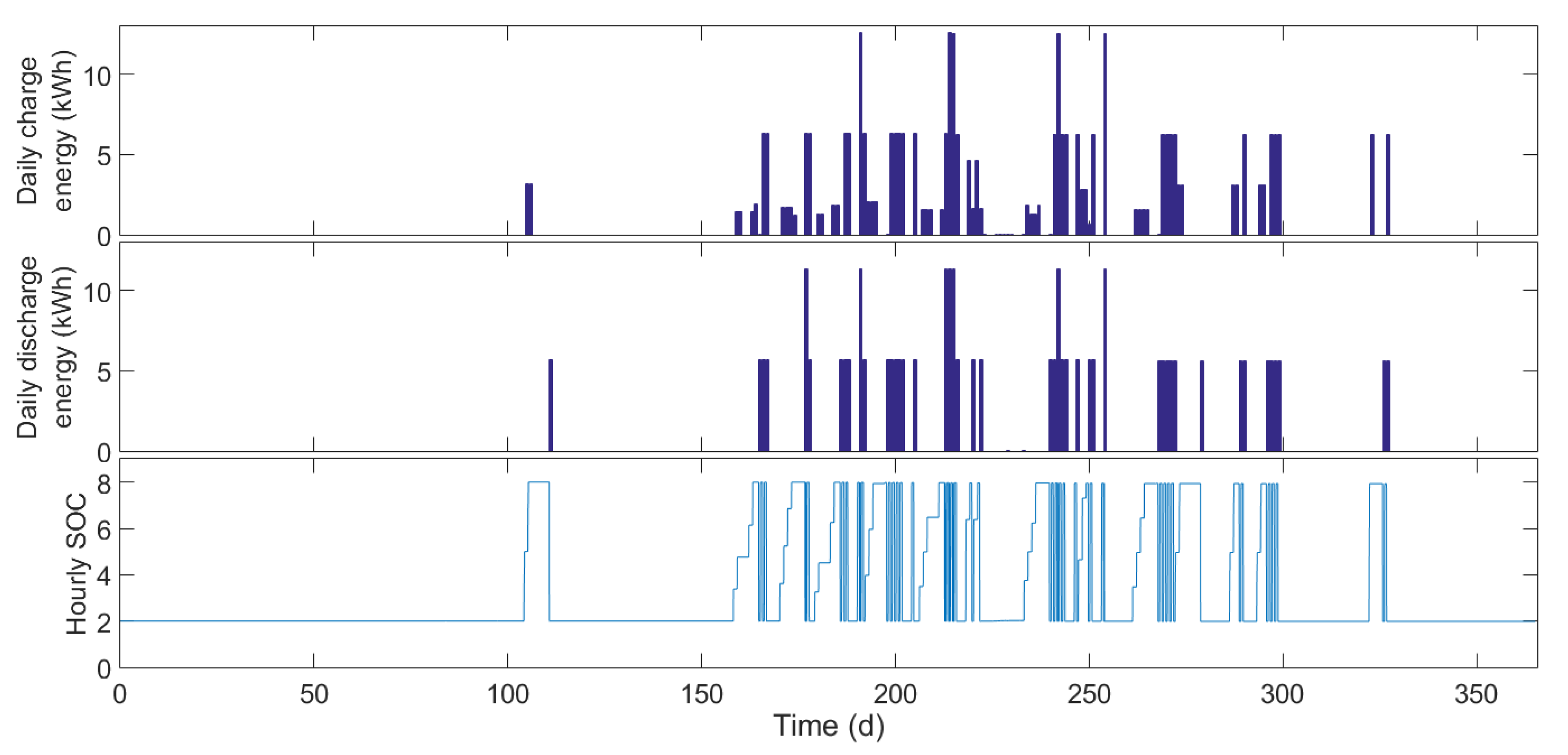
The optimal operation for the battery under the previous assumptions and an assumed battery price of 300 USD/kWh, is shown in Figure 7. As expected, the strategy is to use the energy stored in the battery during the days where the temperature falls in the blue, yellow, orange and red zones indicated in Figure 6, and these are not weekends. This strategy is appreciated in the “Daily discharge energy” subplot, where the total amount of power supplied by the battery to the load during a day () is shown. To allow this operation, the battery initiates its charge in the previous days, in some cases distributing it within several days. This effect is clearly seen around day 175 and the stair-like progression in the SOC subplot, and is affected by the value assumed for in Equation (28). The extreme case where is unbounded is discussed in the Supplementary Information (S4.1), and justifies including Equation (28) in the set of restrictions.
An interesting feature is that the battery is not used in every viable day. Instead, battery usage is concentrated towards the end of the simulation time-frame as shown in Figure 8. We interpret this result as a strategy to preserve battery life, a behavior consistent with the fact that the profit from using the battery at each time depends on its leftover capacity. The rationale is as follows: each day that the battery is used implies a loss in battery capacity that diminishes future profits. Days that provide a high profit are clearly always active. However, days that provide a low profit, become active only when the effect of capacity loss over the profit of future active days is counterbalanced by the (low) profit obtained by using the battery at the present day. This condition is more difficult to achieve at the beginning of the simulation, thus low profit days become active only at the end of the simulation time-frame when there are no more possible high profit future days. This effect is verified by running simulations with different simulation time-frames and costs. As expected, as the batteries become more economical, more moderate-priced days become active at earlier times in the simulation, and as the simulation time-frame diminishes, the active days plots become denser. For the interested reader, these plots are shown in Supplementary Materials. At this point, it has to be noticed that despite being logical, a formal proof of strict convexity of the problem is required to guarantee the uniqueness of the strategy discussed in here.
The net savings considering battery degradation over the operation period are 1006, 977 and 953 USD for 200, 250 and 300 USD/kWh battery costs respectively. Compared to Section 4.2, the difference is not only due to the difference in , but also in the operation scheduling ( and ) and so in battery degradation (). Table 3 shows the yearly savings in electricity bills and the annual loss of capacity for different capital costs. Note that electricity savings are similar for each battery cost, because the extra days that the battery is active add little savings.
5. Conclusions
With the advent of renewable energies, inclusion of batteries as self-storage devices provides an intermediate solution between demand response and grid-level energy storage. In order for this strategy to be widely adopted by small and medium size consumers, a balance between the savings in electricity bills and the cost of replacing the battery must be achieved. In this paper, a new model for optimal battery operation, that includes induced capacity loss due to charge/discharge processes, and its accumulation over time, was developed.
The original problem was relaxed to a convex problem that guarantees global optimality and allows for running the simulations over long time-frames. All the assumptions made in order to relax the original to a convex problem were checked, and are valid as long as battery efficiencies can be considered constant.
The model developed in here allows studying the convenience or not of the installation of a battery-based energy storage system in a residential or small-scale business setting. The model was used to predict the behavior of a Li-ion battery under the assumption of a simple two-price-step day-invariant TOU pricing policy, and a complex temperature-day-season dependent one.
The results of our simulations suggest that simple tariffs, where the price is constant for a large range of hours, operate so that service life is preserved. This preservation is accomplished by charging and discharging every day at very low rates. Our simulations also show that there is a turning point in the cost of the battery that makes the operation not worth. This is, the savings in electricity bill do not compensate the penalization due to capacity loss. This effect is seen even when running the one-day problem, and may be regarded as a first indicator of whether or not it is reasonable to install a battery. For the prices considered in this paper, this turning point is in between 400–500 USD/kWh. Nevertheless, having a battery cost below the turning point does not imply that installing a battery is profitable: positive values for a 10-year lifespan, usual discount rates, and the assumptions made in this case study, are obtained only if the battery price falls below 140 USD/kWh.
For the case of complex tariffs our simulations show that for the same battery price, savings achieved in some individual days could be higher than those of the simple case. However, these savings are counterbalanced with the fact that the battery is not used on a regular (daily) basis. Overall, the battery for the complex tariff considered here is used at most 90 days of the year. Another feature of relevance when considering complex tariffs is that limiting the desired time span between charge and discharge becomes an important input parameter of the optimization problem.
Overall the conclusion is that current Li-ion battery prices (in the order of 500 USD/kWh) and TOU pricing policies are still not attractive enough for acquisition by residential/small-scale consumers. However, as Li-ion batteries systems still have margin to lower their production costs and battery prices are expected to decrease in the near future, small variations in tariff policies may make a difference to favor the installation of this energy storage solutions.
Supplementary Materials
Available online at https://0-www-mdpi-com.brum.beds.ac.uk/2227-9717/6/10/204/s1.
Author Contributions
A.I.T. is the PhD Advisor of M.C. Problem conceptualization, methodology, and formal analysis were developed by discussions between the two authors. M.C. developed the code and run the simulations under the supervision of A.I.T. Both authors contributed equally to the analysis of the results, writing and editing the manuscript.
Funding
This research received funding from Universidad de la República (UdelaR)–Montevideo, Uruguay.
Acknowledgments
Mariana Corengia and Ana I. Torres gratefully acknowledge the Comisión Sectorial de Investigación Científica–UdelaR for the incentive “Dedicación Total” and several travel grants. Ana I. Torres gratefully acknowledges the Sistema Nacional de Investigadores for the economic incentive. Both authors would like to express their appreciation to Juan Andrés Bazerque, Instituto de Ingeniería Eléctrica, UdelaR, for bringing to their attention publications that enriched this work.
Conflicts of Interest
The authors declare no conflict of interest.
Abbreviations
The following abbreviations are used in this manuscript:
| optimization total period of time | |
| battery charging efficiency | |
| battery discharging efficiency | |
| time step | |
| energy storage installed capacity (energy units) | |
| initial energy storage installed capacity (electrical charge units) | |
| energy storage capacity at t (energy units) | |
| dimensionless charge/discharge rate | |
| market cost of battery capacity | |
| terminal potential difference at time t | |
| open circuit potential difference at time t | |
| net current at time t | |
| maximum safe charging power | |
| charge power at time t | |
| maximum safe discharging power | |
| discharge power at time t | |
| r | discount rate |
| state of charge at time t | |
| Minimum required state of charge | |
| Maximum allowed state of charge | |
| fraction of capacity loss during the time step at t | |
| Energy grid price at time t |
References
- Castillo, A.; Gayme, D.F. Grid-scale energy storage applications in renewable energy integration: A survey. Energy Convers. Manag. 2014, 87, 885–894. [Google Scholar] [CrossRef]
- Morales, J.M.; Conejo, A.J.; Madsen, H.; Pinson, P.; Zugno, M. Facilitating Renewable Integration by Demand Response. In Integrating Renewables in Electricity Markets: Operational Problems; Morales, J.M., Conejo, A.J., Madsen, H., Pinson, P., Zugno, M., Eds.; Springer: Boston, MA, USA, 2014; pp. 289–329. [Google Scholar]
- Conejo, A.J.; Sioshansi, R. Rethinking restructured electricity market design: Lessons learned and future needs. Int. J. Electr. Power Energy Syst. 2018, 98, 520–530. [Google Scholar] [CrossRef]
- Mayer, K.; Trück, S. Electricity markets around the world. J. Commod. Mark. 2018, 9, 77–100. [Google Scholar] [CrossRef]
- Samad, T.; Kiliccote, S. Smart grid technologies and applications for the industrial sector. Comput. Chem. Eng. 2012, 47, 76–84. [Google Scholar] [CrossRef]
- Weitzel, T.; Glock, C.H. Energy management for stationary electric energy storage systems: A systematic literature review. Eur. J. Oper. Res. 2018, 264, 582–606. [Google Scholar] [CrossRef]
- United States Department of Energy–Office of Energy Efficiency and Renewable Energy. 2016–2020 Strategic Plan and Implementation Framework. Available online: https://www.energy.gov/ (accessed on 15 August 2018).
- International Energy Agency. Global EV Outlook 2017. Available online: https://www.iea.org/ (accessed on 10 August 2018).
- Reniers, J.M.; Mulder, G.; Ober-Blöbaum, S.; Howey, D.A. Improving optimal control of grid-connected lithium-ion batteries through more accurate battery and degradation modelling. J. Power Sources 2018, 379, 91–102. [Google Scholar] [CrossRef] [Green Version]
- Zhao, Y.; Choe, S.Y.; Kee, J. Modeling of degradation effects and its integration into electrochemical reduced order model for Li(MnNiCo)O2/Graphite polymer battery for real time applications. Electrochim. Acta 2018, 270, 440–452. [Google Scholar] [CrossRef]
- Zhao, X.; Bi, Y.; Choe, S.Y.; Kim, S.Y. An integrated reduced order model considering degradation effects for LiFePO4/graphite cells. Electrochim. Acta 2018, 280, 41–54. [Google Scholar] [CrossRef]
- Sarker, M.R.; Murbach, M.D.; Schwartz, D.T.; Ortega-Vazquez, M.A. Optimal operation of a battery energy storage system: Trade-off between grid economics and storage health. Electr. Power Syst. Res. 2017, 152, 342–349. [Google Scholar] [CrossRef]
- Yan, G.; Liu, D.; Li, J.; Mu, G. A cost accounting method of the Li-ion battery energy storage system for frequency regulation considering the effect of life degradation. Prot. Control Mod. Power Syst. 2018, 3, 4. [Google Scholar] [CrossRef] [Green Version]
- Hu, X.; Martinez, C.M.; Yang, Y. Charging, power management, and battery degradation mitigation in plug-in hybrid electric vehicles: A unified cost-optimal approach. Mech. Syst. Signal Process. 2017, 87, 4–16. [Google Scholar] [CrossRef]
- Zubi, G.; Dufo-López, R.; Carvalho, M.; Pasaoglu, G. The lithium-ion battery: State of the art and future perspectives. Renew. Sustain. Energy Rev. 2018, 89, 292–308. [Google Scholar] [CrossRef]
- Crompton, T.R. 1–Introduction to battery technology. In Battery Reference Book, 3rd ed.; Crompton, T., Ed.; Newnes: Oxford, UK, 2000; pp. 1–64. [Google Scholar]
- Delacourt, C.; Safari, M. Mathematical Modeling of Aging of Li-Ion Batteries. In Physical Multiscale Modeling and Numerical Simulation of Electrochemical Devices for Energy Conversion and Storage: From Theory to Engineering to Practice; Franco, A.A., Doublet, M.L., Bessler, W.G., Eds.; Springer: London, UK, 2016; pp. 151–190. [Google Scholar]
- Jabr, R.A.; Karaki, S.; Korbane, J.A. Robust Multi-Period OPF With Storage and Renewables. IEEE Trans. Power Syst. 2015, 30, 2790–2799. [Google Scholar] [CrossRef]
- Castillo, A.; Gayme, D.F. Profit maximizing storage allocation in power grids. In Proceedings of the 52nd IEEE Conference on Decision and Control, Florence, Italy, 10–13 December 2013; pp. 429–435. [Google Scholar] [CrossRef]
- Fortenbacher, P.; Andersson, G. Battery degradation maps for power system optimization and as a benchmark reference. In Proceedings of the 2017 IEEE Manchester PowerTech, Manchester, UK, 18–22 June 2017; pp. 1–6. [Google Scholar] [CrossRef]
- Ruan, Y.; Song, X.; Fu, Y.; Song, C.; Battaglia, V. Structural evolution and capacity degradation mechanism of LiNi0.6Mn0.2Co0.2O2 cathode materials. J. Power Sources 2018, 400, 539–548. [Google Scholar] [CrossRef]
- Barré, A.; Deguilhem, B.; Grolleau, S.; Gérard, M.; Suard, F.; Riu, D. A review on lithium-ion battery ageing mechanisms and estimations for automotive applications. J. Power Sources 2013, 241, 680–689. [Google Scholar] [CrossRef]
- GAMS Documentation of IPOPT. Available online: https://www.gams.com/ (accessed on 26 September 2018).
- UTE. Pliego Tarifario 2018. Available online: https://portal.ute.com.uy (accessed on 7 May 2018).
- Southern California Edison. TOU-GS-2-RTP. Available online: https://www.sce.com/ (accessed on 20 February 2018).
- ANEEL. Tarifa Branca. Available online: http://www.aneel.gov.br/tarifa-branca (accessed on 20 August 2018).
- MidAmerican Energy. Electric Tariffs Iowa. Available online: https://www.midamericanenergy.com (accessed on 20 August 2018).
- LAZARD. LAZARD’s Levelized Cost of Storage Analysis—Version 3.0. Technical Report. 2017. Available online: https://www.lazard.com/perspective/levelized-cost-of-storage-2017/ (accessed on 9 July 2018).
- Asif, A.; Singh, R. Further Cost Reduction of Battery Manufacturing. Batteries 2017, 3, 17. [Google Scholar] [CrossRef]
- AccuWeather. Available online: https://www.accuweather.com (accessed on 15 August 2018).
Figure 1.
Schematic representation of energy fluxes from the grid to the load. The load can consume energy directly from the grid or from a previously charged battery. represents the power at time t (superscripts C and D denote charge and discharge processes); represent battery efficiencies.
Figure 1.
Schematic representation of energy fluxes from the grid to the load. The load can consume energy directly from the grid or from a previously charged battery. represents the power at time t (superscripts C and D denote charge and discharge processes); represent battery efficiencies.

Figure 2.
Optimal operation for a “simple tariff” example during a 24 h period. (a) Electricity TOU tariff for Uruguay. (b) Optimal power consumed (, represented as negative for visual purposes) and supplied () by the battery. (c) Battery State of Charge at each time (). (d) Fraction of capacity lost by the battery at each time (). Accumulated fraction loss in one day is 1.7 × 10⁻⁴ for 300 and 400 USD/kWh.

Figure 3.
Example of “complex” tariff with different day types and hourly changes. (a) Days presenting a large price variation. (b) Days presenting a moderate variation.
Figure 3.
Example of “complex” tariff with different day types and hourly changes. (a) Days presenting a large price variation. (b) Days presenting a moderate variation.

Figure 4.
Optimal operation for a “complex tariff” example during a 24 h period, for the days that present a large price variation. : optimal power consumed from the grid (represented as negative for visual purposes) and : optimal power supplied by the battery (positive). (a) Extremely Hot Summer Weekday. (b) Very Hot Summer Weekday. (c) Hot Summer Weekday. (d) High cost Winter Weekday.

Figure 5.
Optimal operation for a “simple tariff” example during a 10 years period. (a) (negative) and (positive). Left: First day. Right: Last day. (b) Remaining capacity .
Figure 5.
Optimal operation for a “simple tariff” example during a 10 years period. (a) (negative) and (positive). Left: First day. Right: Last day. (b) Remaining capacity .

Figure 6.
2017 temperature (*) vs. Average temperature (line) in Los Angeles, CA [30]. Each background color implies a different daily tariff. Only seasonal and temperature effects on tariff are considered.
Figure 6.
2017 temperature (*) vs. Average temperature (line) in Los Angeles, CA [30]. Each background color implies a different daily tariff. Only seasonal and temperature effects on tariff are considered.

Figure 7.
Optimal operation for a “complex tariff” example during a year period and a battery price of 300 USD/kWh.
Figure 7.
Optimal operation for a “complex tariff” example during a year period and a battery price of 300 USD/kWh.

Figure 8.
Optimal operation for a “complex tariff” example during a five years period and a battery price of 250 USD/kWh. Notice how battery operation is concentrated towards the end of the simulation period.
Figure 8.
Optimal operation for a “complex tariff” example during a five years period and a battery price of 250 USD/kWh. Notice how battery operation is concentrated towards the end of the simulation period.


Table 1.
Electricity annual savings for each operation year with example simple tariff.
| Operation Year | 1 | 2 | 3 | 4 | 5 | 6 | 7 | 8 | 9 | 10 |
|---|---|---|---|---|---|---|---|---|---|---|
| Annual savings (USD) | 305 | 286 | 269 | 252 | 237 | 222 | 208 | 196 | 184 | 172 |
Table 2.
Simple tariff net present values for different battery prices and rates.
| (USD/kWh) | (USD) | (USD) | (USD) |
|---|---|---|---|
| 400 | −2374 | −2497 | −2606 |
| 300 | −1374 | −1497 | −1606 |
| 200 | −374 | −497 | −606 |
| 150 | 126 | 3 | −106 |
| 100 | 626 | 503 | 394 |
Table 3.
Electricity annual savings and annual capacity loss for each operation year with complex tariff.
Table 3.
Electricity annual savings and annual capacity loss for each operation year with complex tariff.
| (USD/kWh) | Year 1 | Year 2 | Year 3 | Year 4 | Year 5 |
|---|---|---|---|---|---|
| Electricity annual savings (USD/year) | |||||
| 200 | 223 | 230 | 230 | 226 | 223 |
| 250 | 223 | 220 | 218 | 221 | 226 |
| 300 | 223 | 220 | 218 | 216 | 214 |
| Annual capacity loss (%) | |||||
| 200 | 0.96 | 1.29 | 1.37 | 1.35 | 1.34 |
| 250 | 0.94 | 0.93 | 0.93 | 1.09 | 1.34 |
| 300 | 0.94 | 0.93 | 0.92 | 0.92 | 0.91 |
© 2018 by the authors. Licensee MDPI, Basel, Switzerland. This article is an open access article distributed under the terms and conditions of the Creative Commons Attribution (CC BY) license (http://creativecommons.org/licenses/by/4.0/).
Share and Cite
MDPI and ACS Style
Corengia, M.; Torres, A.I. Effect of Tariff Policy and Battery Degradation on Optimal Energy Storage. Processes 2018, 6, 204. https://0-doi-org.brum.beds.ac.uk/10.3390/pr6100204
AMA Style
Corengia M, Torres AI. Effect of Tariff Policy and Battery Degradation on Optimal Energy Storage. Processes. 2018; 6(10):204. https://0-doi-org.brum.beds.ac.uk/10.3390/pr6100204
Chicago/Turabian StyleCorengia, Mariana, and Ana I. Torres. 2018. "Effect of Tariff Policy and Battery Degradation on Optimal Energy Storage" Processes 6, no. 10: 204. https://0-doi-org.brum.beds.ac.uk/10.3390/pr6100204
Note that from the first issue of 2016, this journal uses article numbers instead of page numbers. See further details here.