Lower Limb Exoskeleton for Rehabilitation with Improved Postural Equilibrium


1
Department of Control and Computer Engineering, Politecnico di Torino, Corso Duca degli Abruzzi 24, 10129 Torino, Italy
2
Department of Management and Production Engineering, Politecnico di Torino, Corso Duca degli Abruzzi 24, 10129 Torino, Italy
*
Author to whom correspondence should be addressed.
†
These authors contributed equally to this work.
Robotics 2018, 7(2), 28; https://0-doi-org.brum.beds.ac.uk/10.3390/robotics7020028
Submission received: 28 March 2018
/
Revised: 29 May 2018
/
Accepted: 4 June 2018
/
Published: 8 June 2018
Abstract
:In this work we present a lower limb haptic exoskeleton suitable for patient rehabilitation, specifically in the presence of illness on postural equilibrium. Exoskeletons have been mostly conceived to increase strength, while in this work patient compliance with postural equilibrium enhancement is embedded. This is achieved with two hierarchical feedback loops. The internal one, closing the loop on the joint space of the exoskeleton offers compliance to the patient in the neighborhood of a reference posture. It exploits mechanical admittance control in a position loop, measuring the patient’s Electro Miographical () signals. The problem is solved using multi variable robust control theory with a two degrees of freedom setting. A second control loop is superimposed on the first one, operating on the Cartesian space so as to guarantee postural equilibrium. It controls the patient’s Center of Gravity () and Zero Moment Point () by moving the internal loop reference. Special attention has been devoted to the mechanical multi-chain model of the exoskeleton which exploits Kane’s method using the Autolev symbolic computational environment. The aspects covered are: the switching system between single and double stance, the system’s non-holonomic nature, dependent and independent joint angles, redundancy in the torque controls and balancing weight in double stance. Physical experiments to validate the compliance method based on admittance control have been performed on an elbow joint at first. Then, to further validate the haptic interaction with the patient in a realistic situation, experiments have been conducted on a first exoskeleton prototype, while the overall system has been simulated in a realistic case study.
1. Introduction
Research in biped robotics started in the late 1960s. A huge part of the research has been devoted to exoskeletons [1], haptic mechanical anthropomorphic devices worn by an operator and working in concert with his movements. Complete exoskeletons have been proposed as a promising solution for assisting patients during rehabilitation [2,3]. Even in patients who have lost the ability to autonomously perform certain movements, carrying out assisted exercises of the limbs to be rehabilitated enables the patient initially to regain neural control, and subsequenlty muscular control on that limb. Physiologists call this phenomenon neural plasticity [4]. For example, rehabilitation of the lower limbs to cure patients with post-stroke injuries or Parkinsonian syndromes is used in order to regain or improve posture control and postural equilibrium. Rehabilitation generally requires the patient to carry out a number of repetitive physical exercises, and he needs help, particularly in the early stages of rehabilitation (when the patient has little control of the affected part of the body). Originally assistance was provided manually by one or more therapists. During the last 10 years, rehabilitation systems and apparatuses have been designed, for example harnesses hanging from the ceiling [5,6], that can bear the weight of the patient and constrain him or her to perform the exercises. However, these apparatuses do not involve the patient neurologically or physically. More recently advances in this direction have been achieved by extending these devices so that they can offer force fields and patient cooperative control [7,8].
Pioneering work in lower limb exoskeletons was started by Vukobratovic [9]. He approached the problem of assisting the patient and studied the postural equilibrium of bipeds by introducing the definition of Zero Moment Point (), pointing out the effectiveness of the simple approximation of a linearized inverted pendulum. His results have been widely used in the autonomous biped robotic field, but apparently recent research on exoskeletons has been focused more on increasing the patient’s strength and compliance than on postural equilibrium control [10]. The first example in recent times is BLEEX [11,12] of Berkeley University, which was developed for military application. This device, using inverse dynamics to compute the motor torques, controls hip, knee, and ankle joints in the sagittal plane with no interaction with the operator. RoboKnee [13] controls only the knee, using inverse dynamics without interaction with the user. More recently, in HAL of the Japanese University of Tsukuba and the Cyberdyne Systems Company (Tsukuba, Japan) [14,15,16], the joints at the hip and knee of both legs on the sagittal plane are controlled, while ankles are passive joints. The patient’s Electro Miographical () signals are measured and used to synchronize precomputed walk phases and to modify the mechanical impedance which the exoskeleton presents to the patient [17]. signals have, also, been used by Günter Hommel at the technique university of Berlin for a lower limb orthosis with an actuated knee [18]. The signals enable the effort required of the patient to be estimated and a torque control is performed in order to assist in supporting the patient. In the power Assisting Suit of the Kanagawa Institute of Technology, Japan [19] the control structure calculates the joint torques required to maintain a statically stable pose by computing the inverse of a rigid body model. The current joint angles and the masses of the components of the exoskeleton as well as the weight of the patient are taken into account. Interaction with the exoskeleton is based on the fact that the torques imposed on the joints by the operator overlay with the torques produced by the actuators.
None of the above tackles the two aspects of increasing postural equilibrium (instead of strength) and patient compliance jointly. In fact, the patient’s compliance is based on impedance control (or force control). This means that the patient is potentially free to move and motors at the joints control the torques either by cooperating with his efforts or creating a force tunnel in order to direct his/her movement. Such approaches are not suitable to guarantee postural equilibrium:
- Light weight exoskeletons for walking such as HAL or BLEEX do not even offer enough torques at the joints to support the patient;
- Exoskeletons for rehabilitation on a fixed position such as Lokomat are able to impose a position or a trajectory to the joints, and to offer force fields and patient cooperative control but they are heavy and require a static body weight support.
In both cases the number of controlled degrees of freedom is insufficient to guarantee a posture.
The more recent surveys on the matter are [20,21,22,23,24]. Among the mentioned exoskeletons, REX by Rex Bionics [25] claims postural control. However, no scientific papers have been published and only a patent exists [26], successive to ours [27], without sound scientific descriptions. Moreover REX is not a haptic system. EKSO [28] is an updated version of BLEEX, offering power to people already able to walk. The INDEGO exoskeleton of Parker Hannifin Corporation ([29,30]) is a lightweight exoskeleton offering a rehabilitation modality, called Therapy+, which allows a support, both in static posture and walking, to patients with residual muscular activity. The patient initiates the movement controlling speed, stride length, and step height with as much or as little Indego assistance as needed. Similar is REWALK [31], while MINDWALKER [32] tries to capture the user intention by elaborating eye motion. However, all previously mentioned exoskeletons do not approach the two basic elements of the novel technique presented in this paper: compliance and postural equilibrium control, integrated together.
Compliance has to be achieved by admittance control in a position loop [33,34], and not by impedance i.e., force control, as most of the other approaches do, so that the strength of the position loop enforces postural equilibrium. The multi variable dynamic system has to be considered as a whole, not just some independent joints, controlling at least the minimum number of degrees of freedom to guarantee posture univocally. In this case the exoskeleton maintains the patient in a standing position with a dynamic control, instead of exploiting a static body weight support. Of course, this solution is heavier than the exoskeletons for walking, because the torques needed in this case are from 100 to 200 Nm, instead of 50 Nm. It is, however, lighter than those operating in a fixed position because balancing is achieved dynamically, and not statically.
The proposed exoskeleton is a stationary device not intended for walking but for performing different kinds of postural exercises on a fixed position. The feet are connected to the ground through a kinematical linkage such as a step machine, to offer partial freedom to perform steps. However, further extensions of the approach for walking freely are the object of [35]. Admittance is controlled through EMG signals in order to involve the patient neurologically, programmed and modified by the therapist, while he/she improves his abilities. Lower admittance (i.e., stiffer joints) initially enables passive exercises with the patient bound to the programmed reference postural position or trajectory, and progressively higher admittance eventually consents active exercises: depending on the programmed admittance the patient is able to freely move away from the reference postural position, the control reducing his gravity load. At the same time, postural equilibrium is tutored zeroing admittance and recovering position when limits are reached. To achieve these sometimes conflicting requirements, a first control loop for position and the patient’s compliance has been developed. The loop is based on the measurement of the joint angle position and velocity, and computed with a linear multivariable robust control design in the neighbourhood of a reference postural position, with a two degrees of freedom approach. signals are used to measure the patient’s efforts during motion for compliance and enter the closed loop control as a feedforward signal.
The internal multivariable control guarantees robust dynamical stability and the non-interaction of the patient’s efforts on the different joints for a wide region of the state space. However, dynamical stability does not imply postural equilibrium. A second control loop is superimposed on the first so as to achieve postural equilibrium, based on the concept of “Zero Moment Point” () [36], i.e., the Center of Pressure () of the reaction forces of the floor on a horizontal surface [37]. Physiologists are sceptical about using to control human posture and gait, however a validation using - for walking has recently been published [38]. In reality the objection of physiologists is not on the itself, but in the conservative manner used to control biped robots, originally proposed by Vukobratovic (The always inside the convex hull of the feet support, exploited for equilibrium by the biped robots, is a sufficient condition only. It can be relaxed in certain conditions, leading to an initial free fall).
While the internal loop offers a dynamically stable position control, partially or mostly acted by the patient, postural equilibrium is guaranteed by controlling the during motion (always inside the convex hull of contact points or leaving some freedom according to the dynamics of avoiding to fall). This is achieved by the outer loop controlling the reference postural position of the internal joint loop. The approach adopted for controlling this second loop with analysis for its stability, is the one proposed for autonomous humanoid robot postural control by Choi [39]. It has never been exploited in the context of an exoskeleton with patient interaction, even though recently in [38] the significance of the CoP in the human walk was experimentally validated. Finally, to implement a “step machine”-like exercise, the mechanical model switches between two different phases: double stance and single stance. Hence, specific attention must be devoted to switching the control.
The paper is organized as follows: Section 2 describes the designed exoskeleton and its mechanical model; in Section 3 the general schemes of admittance and postural control are presented; experiments and simulation results for different case studies are presented in Section 4; Section 5 concludes the paper.
2. The Exoskeleton
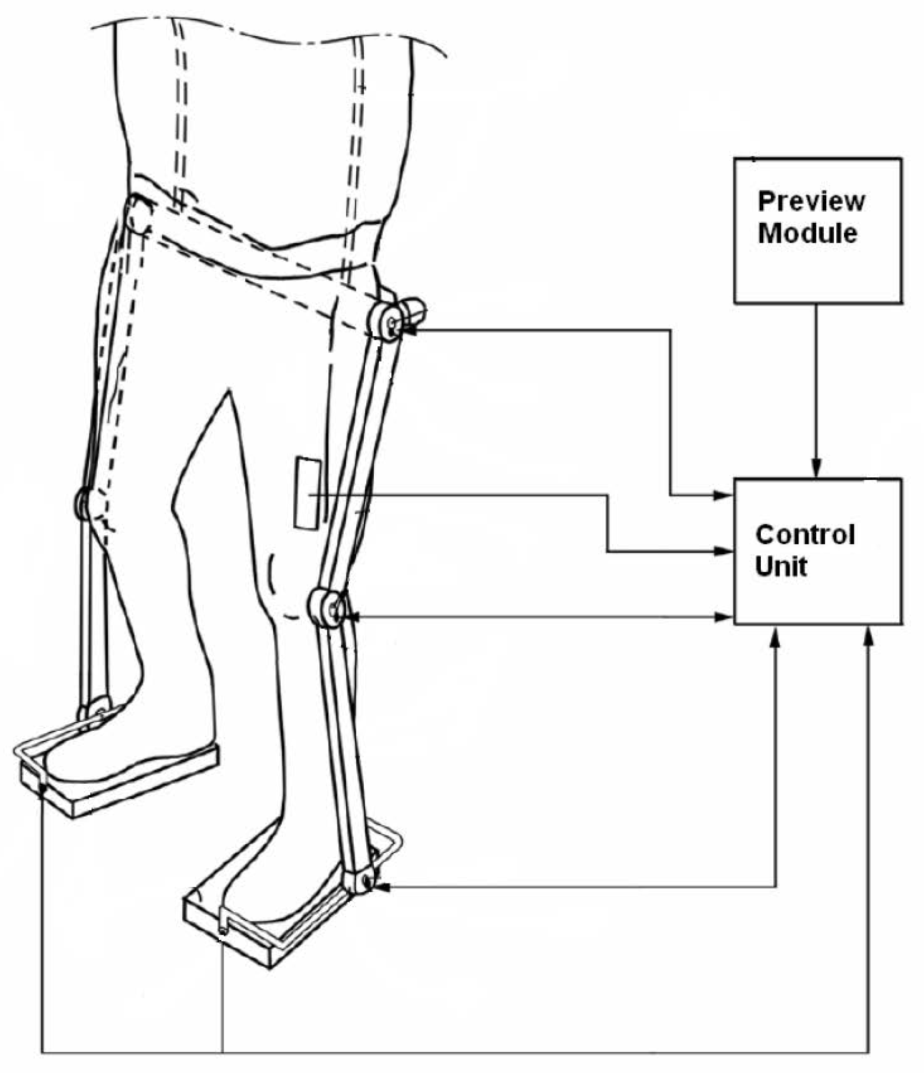
The exoskeleton being considered is represented in Figure 1. Ankle and hip joints have two degrees of freedom, to allow rotation in the sagittal and frontal plane, while the knee has a single degree of freedom, for rotation in the sagittal plane. It is configurated to perform steps in a fixed position, such as a step machine, without the possibility of rotating the trunk along the vertical z axis. Actuators, e.g., electric motors, are coupled to each of the ankle, knee and hip joints. The control unit receives as input: surface signals, from bioelectric sensors coupled to the patient’s lower limbs and placed on the muscles involved in lower limb movement (for simplicity only a thigh sensor is shown in the figure); position and velocity signals from position/velocity sensors, for ankle, knee and hip angle detection; reaction force sensors positioned on the exoskeleton foot rests configured to measure the . While, during single stance, the coordinates of the free foot are derived from the kinematics that links the foot to the ground. Moreover, the control internally generates, with a programmable speed, a preview reference signal for and in the frontal and sagittal planes depending on the rehabilitation exercise. The control unit processes the input signals and, based on the implemented control algorithm, issues suitable driving commands for the electric motors.
The so-called Kane’s method [40] has been adopted for the mechanical modelling. This method deals unitarily with either holonomic or non-holonomic systems, without having to introduce, for non-holonomic systems, Lagrange multipliers. This is particularly useful in this case, because the switching from single to double stance introduces on the same mechanics different non-holonomic constraints.
Briefly, the main contribution of Kane’s method, with the introduction of partial translational velocities and partial angular velocities, generalized active forces and generalized inertia forces, is to determine the dynamical equations, so enabling forces and torques which have no influence on the dynamics to be eliminated early in the analysis. Early elimination of these noncontributing forces and torques greatly simplifies the mathematics and enables problems having greater complexity to be handled.
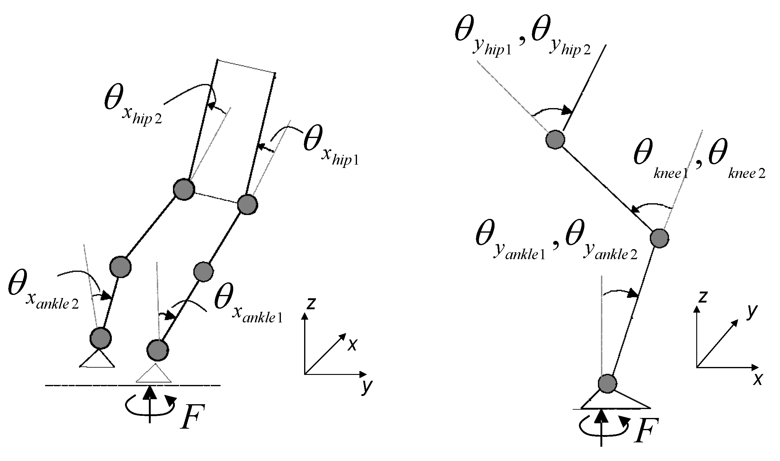
The present exoskeleton is composed of 7 bodies (2 feet, 2 legs, 2 thights and 1 trunk) connected by 10 joints (see Figure 2). Assuming the system to be free to move in the sagittal plane and frontal plane, but not to rotate along the z axis, as is customary in biped robotics, it is characterized by 15 generalized variables and by an identical number of generalized speeds, chosen here as the derivatives of the generalized variables.
Then, according to whether it is in single or double stance, the presence of different non-holonomic costraints, represented by the contact of the foot/feet to the ground, reduces the number of degrees of freedom and offers two distinct models of the dynamics. The model of a biped during a step is, hence, a hybrid dynamical system switching between two different phases, with different inputs and states, described below. Due to lack of space here, the complete modeling approach using Kane’s method and the supporting Autolev environment are described in [41] and can be requested from the authors.
All coordinates refer to Figure 2. Let pedices 1 and 2 be the right and left leg indexes, and use foot 1 as the supporting foot. , are the coordinates of a reference point at the center of the sole of foot 1 and 2 where the reaction forces are conventionally applied. The joint angles indicate as pedices the rotation axis, the joint name and the foot index.
We choose as generalized variables to describe the configuration of the exoskeleton free on the space as the following:
- The three positions in the space of the reference point of foot 1: .
- The two angles of the frame of foot 1: (no rotation along z is allowed).
- The joint angles (as shown in Figure 2): , , , , , , , , , .
The two configurations (single and double stance with independent knees and flat feet) are defined as follows. Conventionally boldface symbols indicate vectors or matrices.
Single Stance: assume that the exoskeleton is sustained by foot 1. Then, the three speeds and two rotational speeds of that foot are zero (motion constraints). In this condition the system has 10 degrees of freedom (5 out of 15 degrees of freedom have been constrained). Moreover, we also impose for simplicity that the second foot is kept flat with respect to the ground. Hence, in the model the degrees of freedom are reduced to 8. One of the possible choices of independent generalized speeds are:
controlled by 8 torques at the corresponding joints:
On the other hand, the 7 motion constraints generate 7 reaction forces/torques: 3 forces applied at the reference point of the supporting foot and 2 torques:
and two torques on the ankle joints of the free foot ( is zero) and . Specifically, these latter torques, which control the free foot, are inessential for the next postural control and they will be ignored here (the problem of controlling the orientation of the free foot can be solved independently of the multivariable control).
Double stance: when the exoskeleton is in double stance, both feet are on the ground. Hence, the system loses 3 more degrees of freedom resulting in 5. A reasonable choice of the independent generalized speeds is:
In this configuration the system needs 5 torques, e.g., at the corresponding joints, as input in order to control its posture, while the remaining 5 torques are redundant.
The reaction forces/torques, present now at both feet, are
Software called Autolev [42] has been adopted in order to perform the symbolic computation requested by Kane’s method. Its outputs are the dynamical equations of the non-linear model of joint motion in the two configurations of single stance and double stance to be used for simulation, as well as the programming code of the expressions for the reaction forces/torques at the constraints returned from the model, the kinematics of and of the free foot, the Jacobian, the Jacobian matrix linking dependent and independent motion variables, to be embedded in the control.
Specifically, in simulation the theoretical expressions for the coordinates for both single and double stance given by the force/torques at the feet returned from the model are:
In the control of the real exosleleton, these coordinates will be given by estimating the from the sensors under the feet, as described in Section 3.2.1.
The dynamics in sagittal and frontal planes are weakly intertwined. So, here, for designing the control these are separated ignoring interactions, and 4 linearized multi input-multi output models in single and double stance on frontal and sagittal planes have been derived. Linearization has been performed with the model in an erect posture, with knees slightly bent. Their states and output are the position and speed of the following joint angles, and the control inputs are the corresponding torques:
- Frontal plane—Single Stance: , , .
- Sagittal plane—Single Stance: , , , , .
- Frontal plane—Double Stance: .
- Sagittal plane—Double Stance: , , , .
3. Compliance and Equilibrium Control
3.1. Position and Admittance Control
Mechanical Impedance [43] is defined as the transfer function (TF) of the linear dynamical operator giving as output the reaction forces/torques in a mechanical system when imposing velocities/angular velocities as input. The inverse of the Mechanical Impedance is called Mechanical Admittance, i.e., the output velocities/angular velocities resulting from the application to a mechanical system of input forces/torques. Integrating on time velocities, by extension the same concept can encompass the relationship between positions and forces or vice versa.
Open loop and closed loop haptic feedback and virtual reality systems have been proposed in the literature to control compliance, based on the previous definitions, but implementations are mostly of the impedance type. However, admittance control in a position loop of the joints [44], applied to an exoskeleton, offers the advantage to keep the system dynamically stable and insensitive to external disturbances (e.g., gravity) on a reference postural position, fixed or moving along a planned trajectory. At the same time, the patient feels the chosen admittance when he tries to deviate from that reference. Examples of planned trajectories in double stance are the exercises of sit-to-stand, this is performed on the sagittal plane with the knees jointly, or reaching the limits of equilibrium by moving the CoP to the toes. A further example is to move in a step like fashion on the frontal plane by translating the weight from one foot to the other, then switching from double to single stance on the supporting foot and lifting the free foot from the ground, and vice versa.
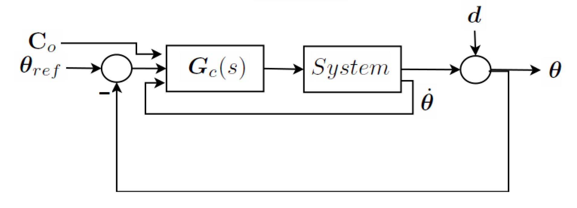
By independently exerting an effort with his/her muscles the patient will be able to move the joints of the exoskeleton away from the reference position by exploiting signals from the leg muscles. In doing so the patient experiences a reaction consistent with the chosen admittance, where the three basic elements-elastic stiffness, frictional and inertial effects-can be independently and dynamically modified for each joint. These results are achieved by a closed loop from joint angle position and velocity measurements, computed with a multivariable robust control design, using signals as feedforward input. The general scheme of control presented here is applied to each one of the 4 models derived in the previous section, according to the phase of the step. At difference to what is proposed in the literature [43,44], the admittance control is performed here in the joint space, esploting non-interactive multivariable control to decuple each joint dynamics. This non-interaction is achieved with a two degree of freedom control, as defined by Horowitz [45]. The two degrees of freedom control (shown in Figure 3) makes it possible to independently specify loop characteristics (i.e., disturbance insensitivity, precision of reference tracking) and admittance in the patient’s compliance, in response to EMG signals, indicative of the efforts. are the reference joint angles, in which neighborhood the efforts measured from the patient allow the exoskeleton joint angles to move. The TF is the desired admittance , for non-interaction a diagonal matrix:
and are the desired stiffness and viscosity of the i-th joint which are felt by the patient (A slight viscous factor is needed to avoid instability in the patient’s response due to unwanted physiological feedback, and to filter EMG signal noises. Inertia for simplicity is set at zero in the desired admittance. However, as the next example will show, an unwanted inertial effect will be introduced by the limited control loop bandwidth). Basically, patient efforts act as measured disturbances to be accommodated (tracked) through feedforward by the control loop. As already stated, in a rehabilitation scheme, the reaction will initially be set stiffer and more compliant later, depending on the patient’s progress, respectively lower and higher steady state gain of the TF.
The technique has been chosen so as to approach the control of all joints as an unitary multivariable system, and in this way to guarantee robustness in the face of the linearization on a large state space region and to offer non-interaction of the efforts on the different joints. The general theory of and of the mu-synthesis design technique, adopted here, can be found in [46,47,48].
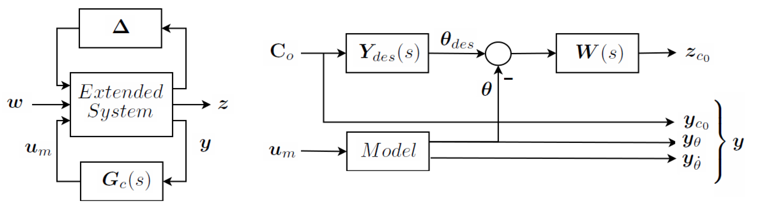
Requirements in a robust control design are set defining an extended system. Input-output performances and robust stability in the presence of uncertainty of this extended system closed by the feedback evaluate the synthesized control , as shown in Figure 4. The extended system encompasses: nominal model, uncertainty description, input noise and control, output measures and performance objectives. In a two degrees of freedom control, to guarantee compliance, it also embeds the measured disturbances, which are the patient’s efforts, the desired admittances and, as objectives, the tracking errors of the outputs of these desired admittances.
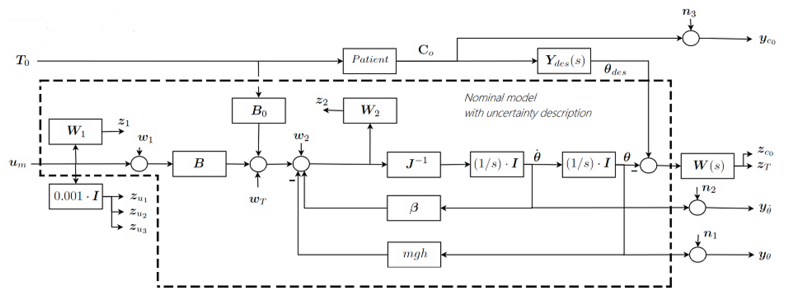
The detailed extended system in our case is presented in Figure 5. The main elements are:
- , the inputs to the motor actuators.
- , the multiplicative uncertainty at numerator representing the ignored motor dynamics, and is the corresponding pair disturbance-objective.
- , the patient torques, measured by the signals.
- the measured signals in output.
- Patient torques and motor torques drive the exoskeleton dynamics, which is modeled by the linearized model equations:where and are the motor and patient torques, is the inertial matrix, the damping matrix, represents the matrix of the linearization of the effects of the gravity forces and the input torque disturbances.
- is the multiplicative uncertainty at the denominator of inertia, to guarantee robustness to non-linearities. and are the corresponding pair disturbance-objective.
- , the diagonal TF matrix of the desired admittances;
- Objectives impose requirements on tracking errors against and on the closed loop sensitivity to input disturbances ; is the diagonal matrix of weighting functions which define the desired loop gain and bandwidth of the control;
- , the objectives penalizing the control activity against the measurement noises ;
- and , the measured joint position and velocities.
Similar schemes, applied to the four models described in the previous section, resulted in four controls: to be switched in pairs (sagittal and frontal plane) moving from single to double stance and vice versa.
As a result of the synthesis, in the limits of the achieved loop gain and bandwidth, the closed loop system will not only be able to reject loop disturbances and track joint angle references, but also to guarantee the desired admittance to the patient.
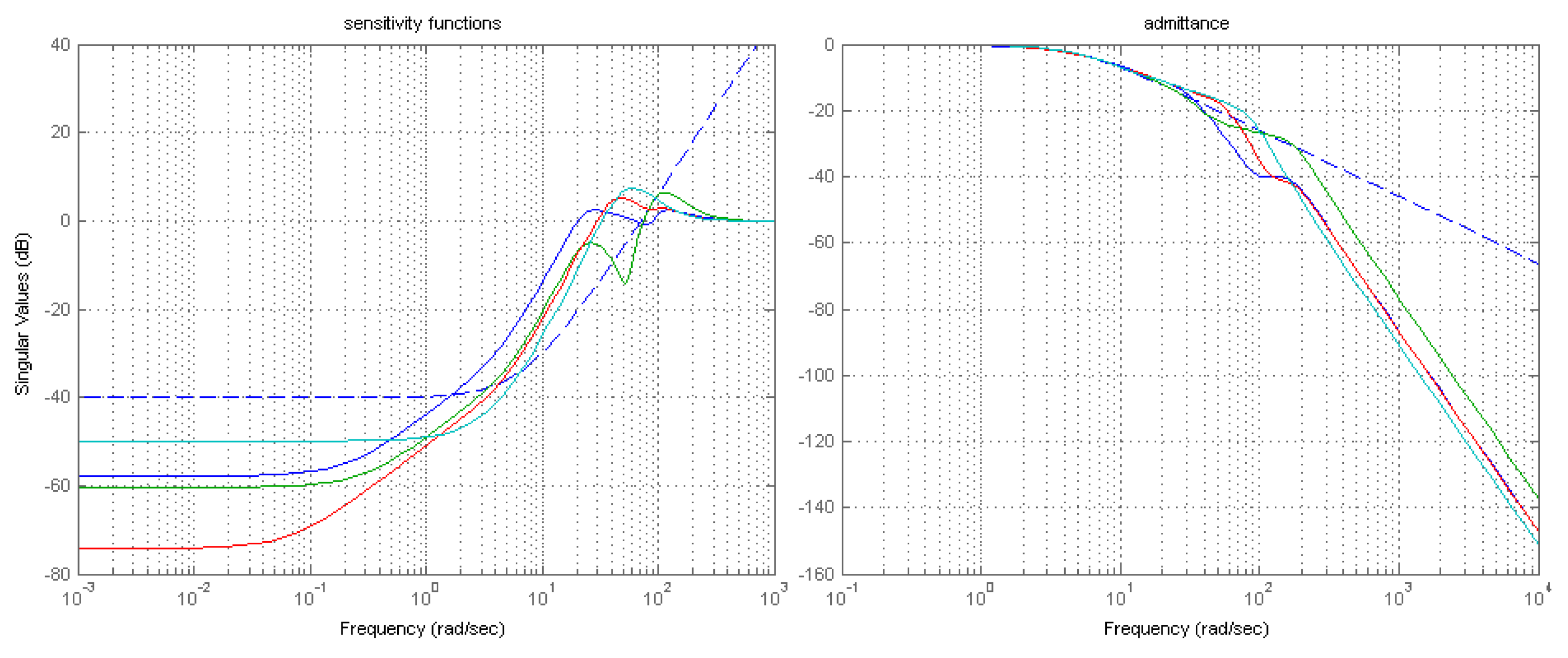
Figure 6 shows the resulting two basic TFs of the extended system in closed loop for one of the linearized models of the exoskeleton discussed in Section 4: achieved represented by continuous lines, specified by dashed lines. This is the phase of double stance in the sagittal plane, with angles , , , . The figure on the left shows the output sensitivities of the four angles ( in Figure 3), indicating an achieved closed loop band of rad/s, and disturbance rejection over −40 dB. The figure on the right outlines the achieved admittances, normalized to a steady state gain equal 1, for the four joints (), non-interaction which is not shown here is almost perfect, i.e., cross-admittances are almost zero. Note that, with respect to other authors dealing with force/torque control with impedance imposed in open loop, here the desired admittance is satisfactorily tracked up to the limit of bandwidth of the feedback loop. The consequence of the limited loop bandwidth is an unwanted inertia perceived by the patient, evident from the deviation of the actual from desired functions.
Performances similar to those of Figure 6 have been obtained for the other phases and planes.
3.2. Postural Equilibrium
In order to guarantee postural equilibrium, the vertical reaction forces of the floor on the feet must remain inside the section of the supporting sole during any postural exercise, or in response to external disturbances. Hence, a second loop is super-imposed on the first one to ensure postural equilibrium. It controls the Zero Moment Point (ZMP) based on Lyapunov stability theory, the Jacobian function of the Center of Gravity (COG) and a linearized inverted pendulum model. It measures reaction forces from sensors on the sole of the exoskeleton and acts on , the reference angles of the previous inner control loop.
3.2.1. Improved COG and ZMP Estimates
To improve the estimation of and we merge a priori knowledge of the multichain with a posteriori measures of the . The model adopted to represent the relationship between and is the linearized inverted pendulum [49]: a pure triple integrator driven fictitiously by the jerk as an input noise. It should be noted that there are two independent identical models of the relationship: one along the x axis (sagittal plane) and one along the y one (frontal plane). In the following, the pedix i in and represents .
where is the average z coordinate of the , g is the acceleration of gravity, is the jerk.
From Equations (9) and (10) estimators, based on two identical Kalman filters, of the / x and y coordinates have been developed. These estimators fuse the theoretical values of and available from joint angle and derivative measures, known the kinematics and Jacobian of the , with coordinates, from the measured by load cells on the soles of the feet.
Outputs of the estimator are , , and its derivative.
3.2.2. Preview Control
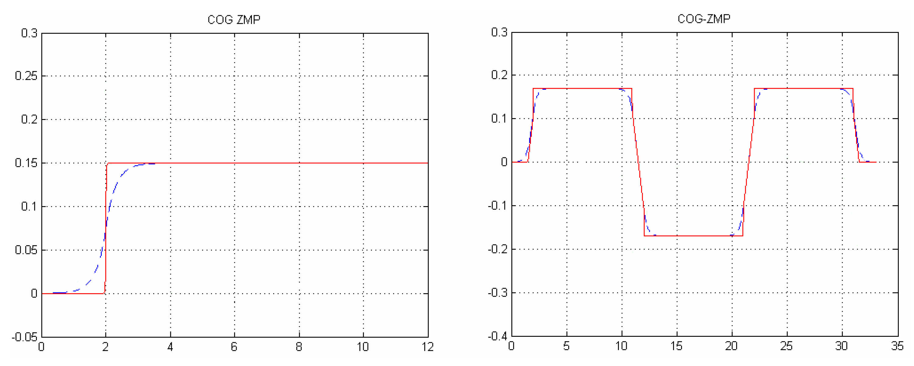
In a quiet standing, references for and remain constant, but if we want to impose, during a postural exercise, a desired trajectory to the , the trajectory must anticipate the transition and be computed in advance, based on an inverted pendulum model. This is called a preview control (for details see [39,49]). Assigning a preview control to the is particularly convenient in the case of rehabilitation exercises, as the trajectories in the exercises are pre-planned and/or periodic. Note that in preview control, the reference position and reference velocity are determined together. In Figure 7 two preview signals are shown: the first represents an exercise on the sagittal plane to reach the limits of equilibrium ( moves to the tips of the feet) and the second is the exercise of the step machine performed on the frontal plane.
3.2.3. Jacobian
Velocities of Cartesian coordinates of the significant points or the attitude of bodies composing a multichain are linked to the joint angle velocities through the Jacobian matrix. It is classical to exploit the inverse of the Jacobian matrix to transfer posture (Cartesian) motion into joint space motion when the vector of the independent Cartesian coordinates has a dimension equal to the number of degrees of freedom of the multichain, and to control a system by Cartesian, instead of joint, references.
However, the number of Cartesian constraints can be more or less than the degrees of freedom, so a pseudo-inverse is used. In the latter case (the Jacobian matrix block row, system over-actuated), e.g., when only the x and y coordinates are constrained, the minimum least squares velocities of the joint angles are determined. In the former (the Jacobian matrix block column, system under-actuated), introducing a relative weight to each row, weighted least squares will offer a solution for the joint motion that is a compromise in satisfying several desired postural variables, or body attitudes.
In this work , , and trunk angles along x and y are constrained, while the patient controls the joint angles directly. Note that this is enough to guarantee postural equilibrium. However, the same method can be extended to cases where additional constraints on the general body posture have to be kept, e.g., swing foot trajectory in single stance. We found it convenient, for simplicity, to ignore the interactions and maintain in the control the two planes (sagittal and frontal) separate. Hence, if (Equations (1) and (4)) are the two vectors of joint angles on the respective planes:
When one or both knees are fully extended, it may be convenient to add to the Equation (11) for the sagittal plane an artificial tutor to the involved knee(s) so as to avoid over stretching of those angles:
where , are the Jacobian of and trunk attitude, and is a 1 or 2 row matrix with only 1 in the columns corresponding to the interested knee joints.
3.2.4. Postural Control Loop
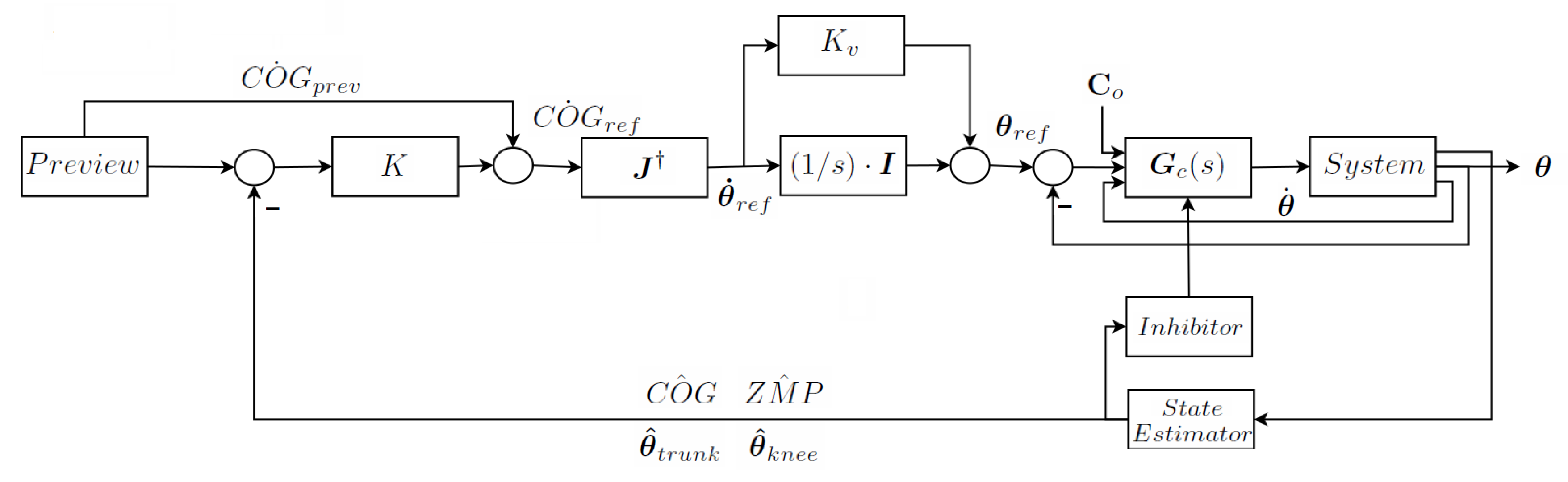
The complete control scheme (one for each plane) is shown in Figure 8. The preview block provides preview , and trajectories. The error between the previews and the estimated signals and is used to generate the velocity in order to close the loop with the following feedback law (block in Figure 8) :
and are gain coefficients. For trunk attitude control, and in the case of a knee tutor, a vector can be formed adding to Equation (13) the following components:
avoiding rotation along x,
imposing a slight forward lean in the sagittal plane, and
constraining knee overstretching.
Then, through the pseudo-inverse of the Jacobian matrices of Equations (11) and (12), by integrating all the components, can be computed.
Choi [39], who proposed the scheme of Equation (13), proved the existence of values for and that guarantee loop stability through the Lyapunov theory. Nevertheless, it is advantageous to add a velocity gain in the loop in parallel to the integrators in order to improve the closed loop poles damping so coping with unmodelled dynamics of the actuators. The reference joint angles become the input of the inner joint position control. Hence, when during the exercise the patient moves the away from the preview value the vector is modified by the feedback and the patient will feel an elastic attraction toward the desired (equilibrium) position. In extreme cases, when a threshold on the and position is being reached an inhibitor dynamically reduces the desired admittance of the internal loop (up to setting it at zero) increasing stiffness in Equation (7), forcing the patient to recover the equilibrium.
3.2.5. Balancing Weight and Admittance Control in Double Stance
In double stance, because of the non-holonomic constraints and reduced degrees of freedom the system is overactuated and some joint torques are redundant. Hence only some of the joints need to be controlled for position and the remaining ones can be advantageously exploited for ground reaction force control. The signals of those joints not controlled in position must be averaged with the others in order to offer the patient a feeling of admittance balanced on each joint.
Reaction Force Control
The proposed exoskeleton has 10 joints; in single stance only 8 need to be controlled: and are inessential for postural control and will be treated separately.
In double stance only 5 joints need to be controlled, the remaining 5 controls, consequently, are redundant. Then, the 10 input torques can be divided in two 5 dimensional vectors, indicated as primary (for position control) and auxiliary respectively, are defined as follows
and indicate the 5 reaction forces/torques returned by the constraints on the right and left foot in Equation (5).
Autolev provides the equations for these reaction forces, which among other nonlinear terms, are linearly dependent of all input torques (primary and auxiliary control variables) and of the motion variable derivatives (accelerations).
Most of those terms are imposed by the motion, but in particular and depend on the auxiliary torques. The 10 ground reaction forces/torques on the two feet cannot assume arbitrary values, as their sum depends on the imposed motion, but their ratio can be controlled by the five components of . Let the desired reference values of these reactions forces/torquers on each foot, during a double stance phase, be
Moving from 0 to 1 represents the transfer of weight from to , and, in particular, is the center balance. The difference of the errors between references and actual values is given by
It can be controlled by , considering that is given by the motion, but
and information of is obtained from and measured through load cells on the soles of the feet (). Then transferring the load from one foot to the other can be achieved by minimizing in real time with a gradient technique, controlling the auxiliary torques with the following iterative scheme
Under mild conditions, there are values of the feedback k that guarantee stability. The recursion converges and reaction forces/torques under the feet behave properly, tracking the desired reference.
This technique is exploited also, switching the control from single to double stance just before the contact of the swing foot with the ground, to offer compliance for managing the collision and accommodating the foot to an uneven floor surface.
Averaging
To cope with redundancy, and the reduced number of independent motion variables the torques measured by EMG signals on independent and dependent joints have to be averaged in order to guarantee a balanced admittance felt on all joints by the patient. This can be achieved as follows.
Identical admittance is imposed on all joints by design. The Laplace transform of the relationship between torques experienced by the patient, as measured by EMG signals, and joint motion is
here is the time derivative of the scalar admittance assumed to be identical to all joints. is the Jacobian between dependent and independent joint velocities. Solving by least squares in Equation (23) shows how the patient torques have to be averaged.
In fact, vector is the input applied as feedforward to control the independent joints.
3.3. Switching between Phases
The controllers of the inner loop, the Jacobian matrix and the integrators of the outer loop must switch, moving from single to double stance and vice versa. This requires setting the correct initial conditions in order to avoid spikes in the controlled torques during the switch. Let us define , and as the joint torques, joint positions and velocities before switching, respectively. Let be the reference joint velocity after switching at the output of the pseudo-inverse of the , and the initial conditions of the integrators. The at the initial condition will be
Consider the digital controller
Selecting a stable controller (which has always been the case in all examples performed), torques before and after the switch are equated, maintaining the controller in steady state:
where . Hence, deriving from Equation (27), considering (25)
4. Experimental Results and Case Studies
In the following subsections, the experimental evolution of the project is presented:
- When a complete lower limb exoskeleton was not yet available, in order to validate the effectiveness of using EMG signals for admittance control, experiments on the forearm of an operator have been performed.
- Then, the first (incomplete) lower limb exoskeleton prototype has been built, and the preliminary experiments results are here documented.
- Finally, the simulation results of the complete behavior of the lower limb postural and compliance multi-variable control are presented.
4.1. Validating EMG Signals for Admittance Control
A prototype of an upper limb exoskeleton with only one joint to control the elbow of a healthy operator has been built, and the technique described in Section 3.1 was implemented. The objective was to test the quality of the EMG signals, the effects of noise, and to verify the differences between the efforts needed to perform identical motions with different imposed admittances.
The operator’s forearm was bound to the exoskeleton with a maintained at with respect to the vertical, and excursion of the forearm from horizontal to vertical was allowed. The EMG signals of the two antagonist muscles, biceps and triceps, were measured with a sampling frequency of 1 KHz, filtered by a band pass filter (100–150 Hz), rectified and further filtered with a low pass filter of 100 rad/s, then, after the amplitudes of the two signals were balanced, the difference was used as input for the controller as in Figure 3.
An offset was added to guarantee that the arm was at rest without effort, and the relative gains of the signals from the two muscles were balanced to offer a similar perceived compliance during motion in both directions.
On the computer display in front of the operator a reference sinusoidal trajectory was plotted in real time, and the measured output of the elbow angle was superimposed. The exercise required the operator to follow with his elbow angle the reference trajectory as closely as possible.
The chosen admittance was
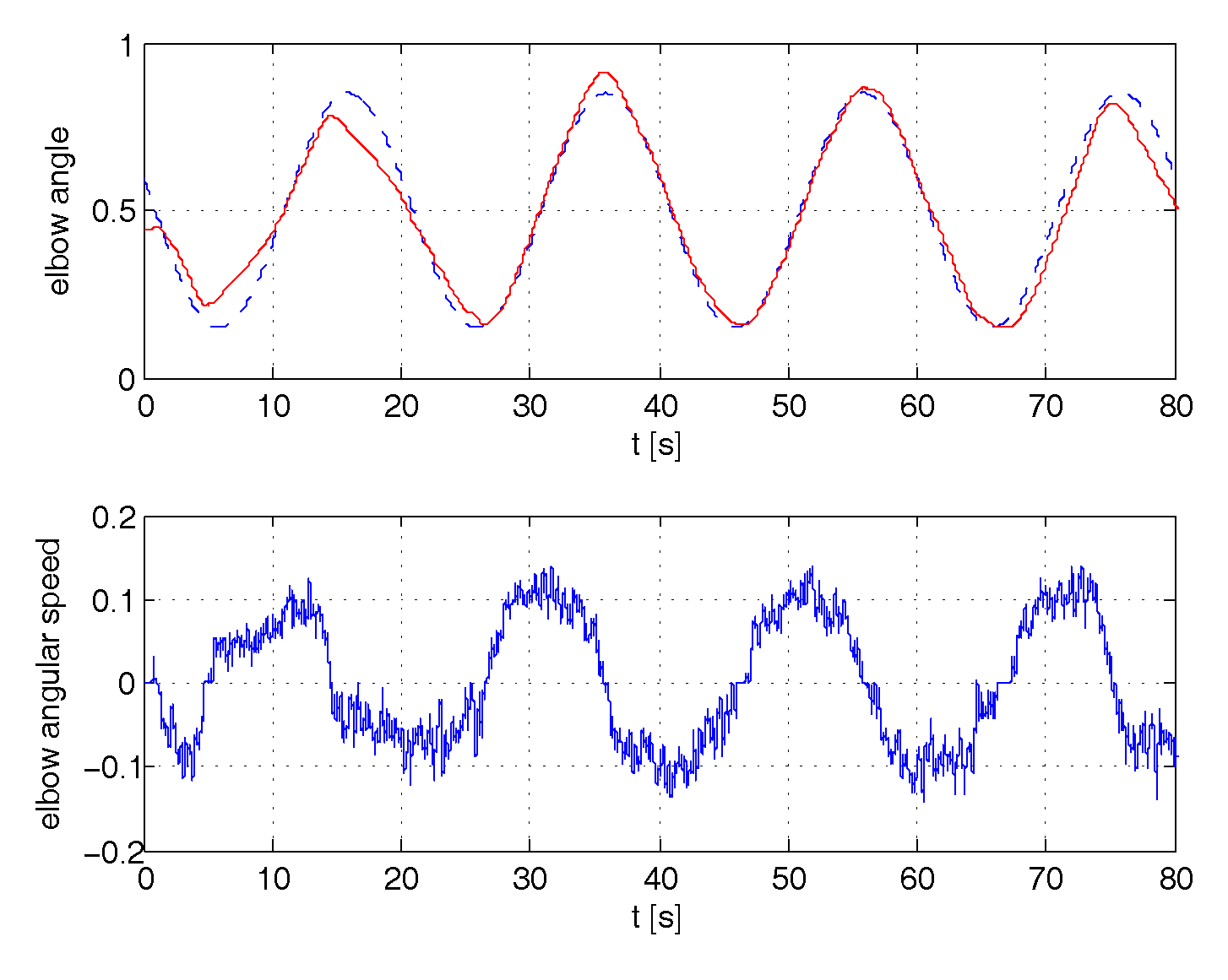
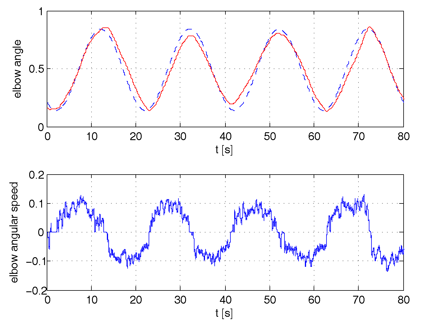
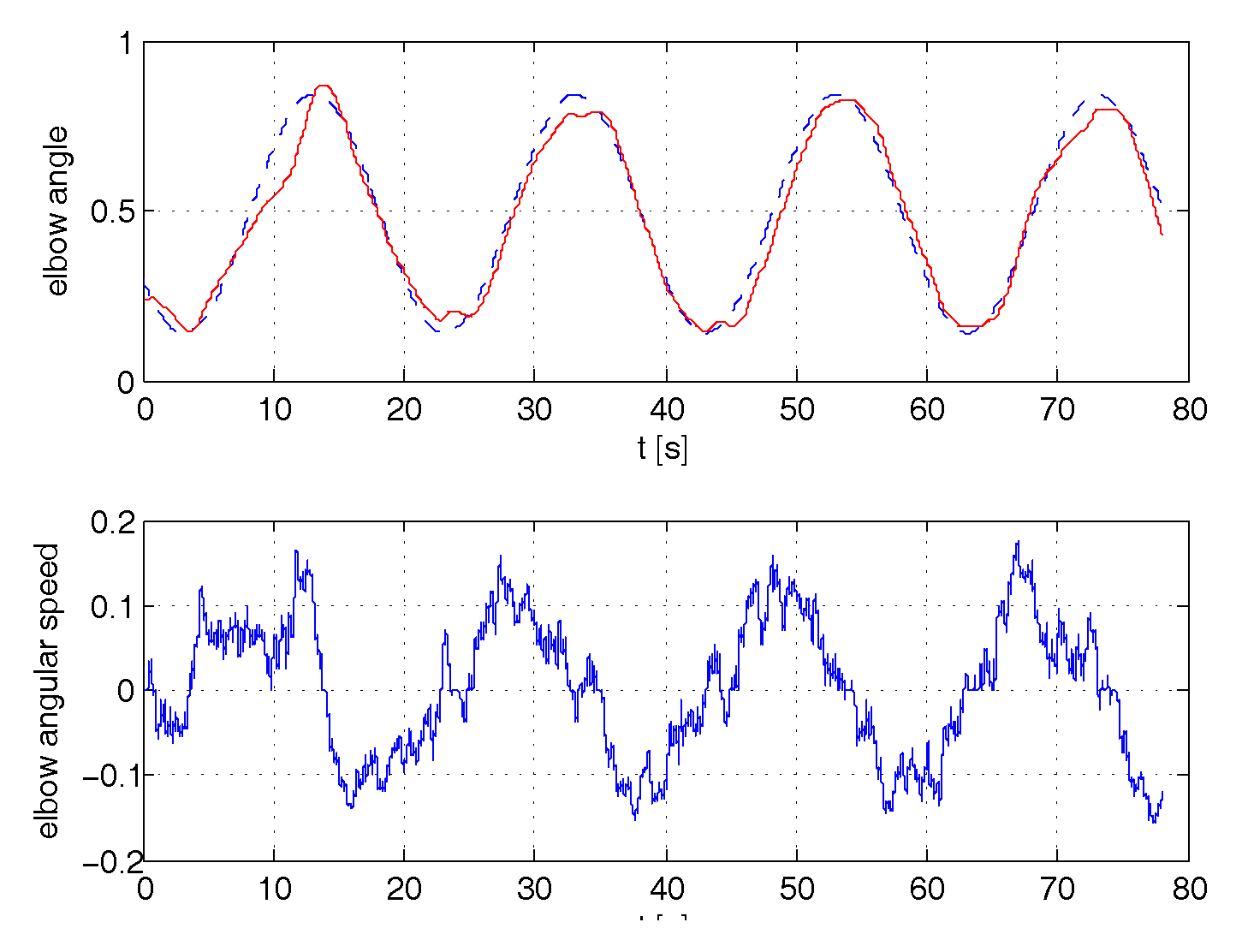
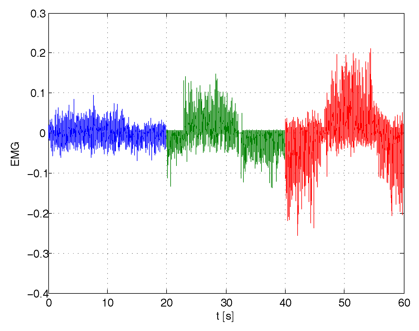
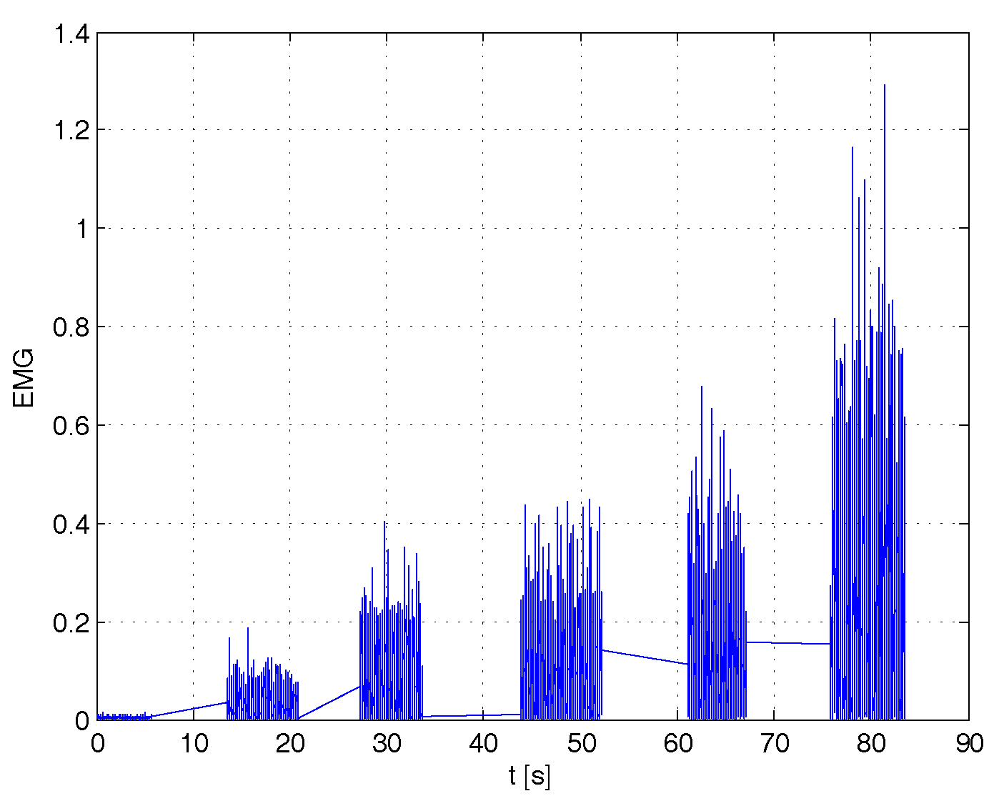
A series of experiments were performed with (no spring stiffness), and values of (friction) ranging from to , 10 times greater. These values represented the maximum and minimum allowable steady state gain of the admittance, respectively due to EMG signal noise, and capability of the operator to still track with an acceptable effort the reference. Correspondingly, the values of j (inertia) were chosen within the range 0.15–0.25 so as to filter noise for maximum operator comfort. These values maintain a frequency band of admittance of approximatively 2 rad/s. The results of angle position tracking and velocity are reported in the Figure 9, Figure 10 and Figure 11. In all cases, the reference sinusoidal trajectory is tracked reasonably well. Samples of the efforts by the operator to perform each exercise, in terms of amplitude of the signals, are extracted from each experiment and merged in Figure 12. The first 20 s refer to the high admittance experiment, while seconds 20–40 and 40–60 refer to the medium and the low one. It can be seen that muscle activation with high admittance is barely detectable from the noise. Nevertheless, the tracking of the angle is still satisfactory. Even though not directly comparable, in order to relate these signal levels to the perceived operator effort, another experiment was conducted on the forearm free from the exoskeleton, held horizontally in an isometric condition. The signals in several successive experiments are recorded in Figure 13: first the forearm was at rest on the table (just signal noise), then it sustained its own weight alone, later weights on the hand of 1,2,3,5 kg were added. The contribution of the exoskeleton can be seen in the case of high admittance, as the level of the EMG signal on performing the exercise of tracking is half that needed to sustain its own weight.
Finally, we carried out a posteriori identification of the admittance perceived by the operator from the pair input EMG signals and output elbow joint velocity and we found that:
- the identified admittance was consistent with the desired one imposed by the control.
- the reconstructed velocity derived applying the noisy EMG signals to the identified admittance was very similar to the measured one.
4.2. Experiments with the First Prototype of the Exoskeleton
To further validate the haptic interaction with the patient in a realistic situation, experiments on a first lower limb exoskeleton prototype have been performed.
4.2.1. Prototype Description
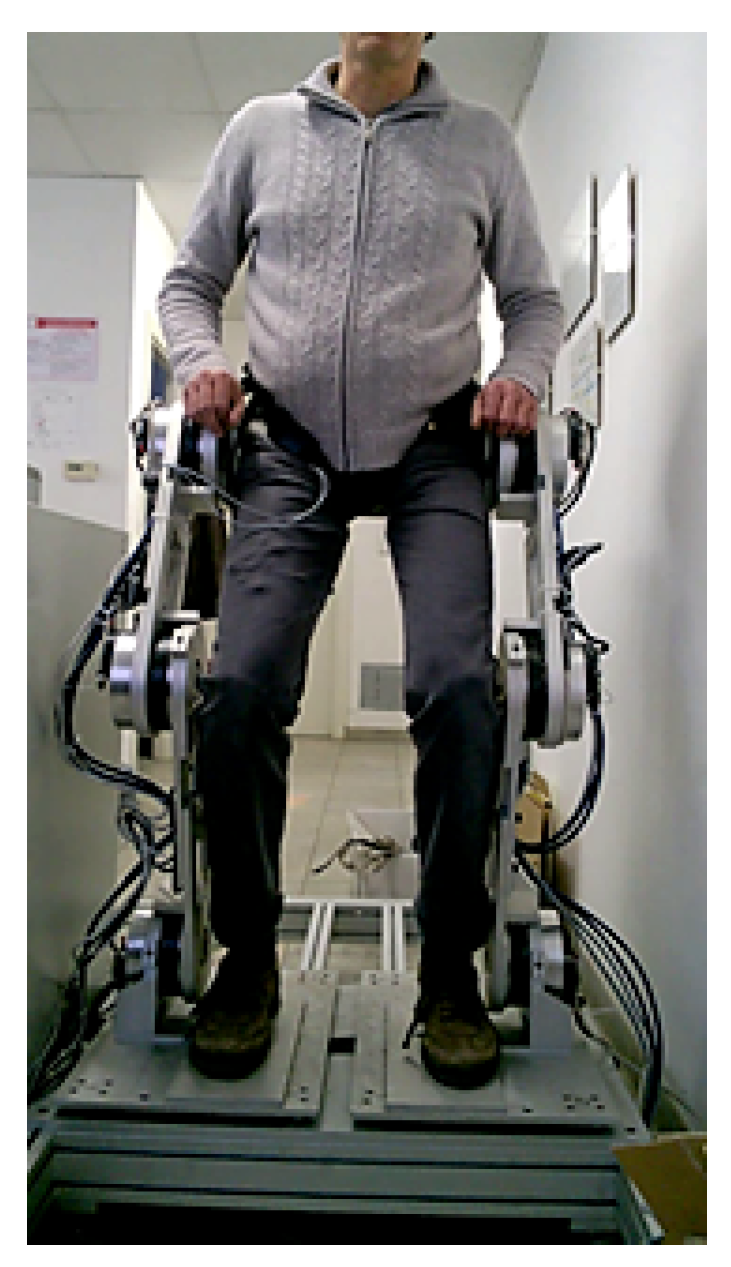
This first prototype (see Figure 14), has been conceived for performing sit-to-stand exercises [50], for testing the lower limb interaction with the patient. The exoskeleton feet are fixed to dynamometric platforms on the ground. The ankles, knees and hips have only one degree of freedom in the sagittal plane. Hence, the sensors and the controls of the right and left legs are paired, allowing three degrees of freedom in the sagittal plane. With this configuration, it is not possible to raise one foot from the ground or to balance the weight alternatively on the two feet (sit-to-stand exercises are possible, while step-like exercises are not). Furthermore, in order to prepare the prototype for future extensions, pressure sensors under the soles of the two feet are separated, measuring the COP in both the sagittal and frontal plane and motors on the joints are independent. The mechanical structure weighs 80 kg, half of that on the supporting platform. Joints are controlled by flat brushless motors of 200 W, with a maximum torque of 1 N·m. As reductors, harmonic drives with a rate of 100 coupled to a further reduction of 5 are used, reaching a maximum torque on the joints of 500 N·m, able to completely support exoskeleton and patient weight in any postural position.
4.2.2. Experiment Preparation
EMG sensors have been fixed on the patient legs, measuring the signals on the following muscles:
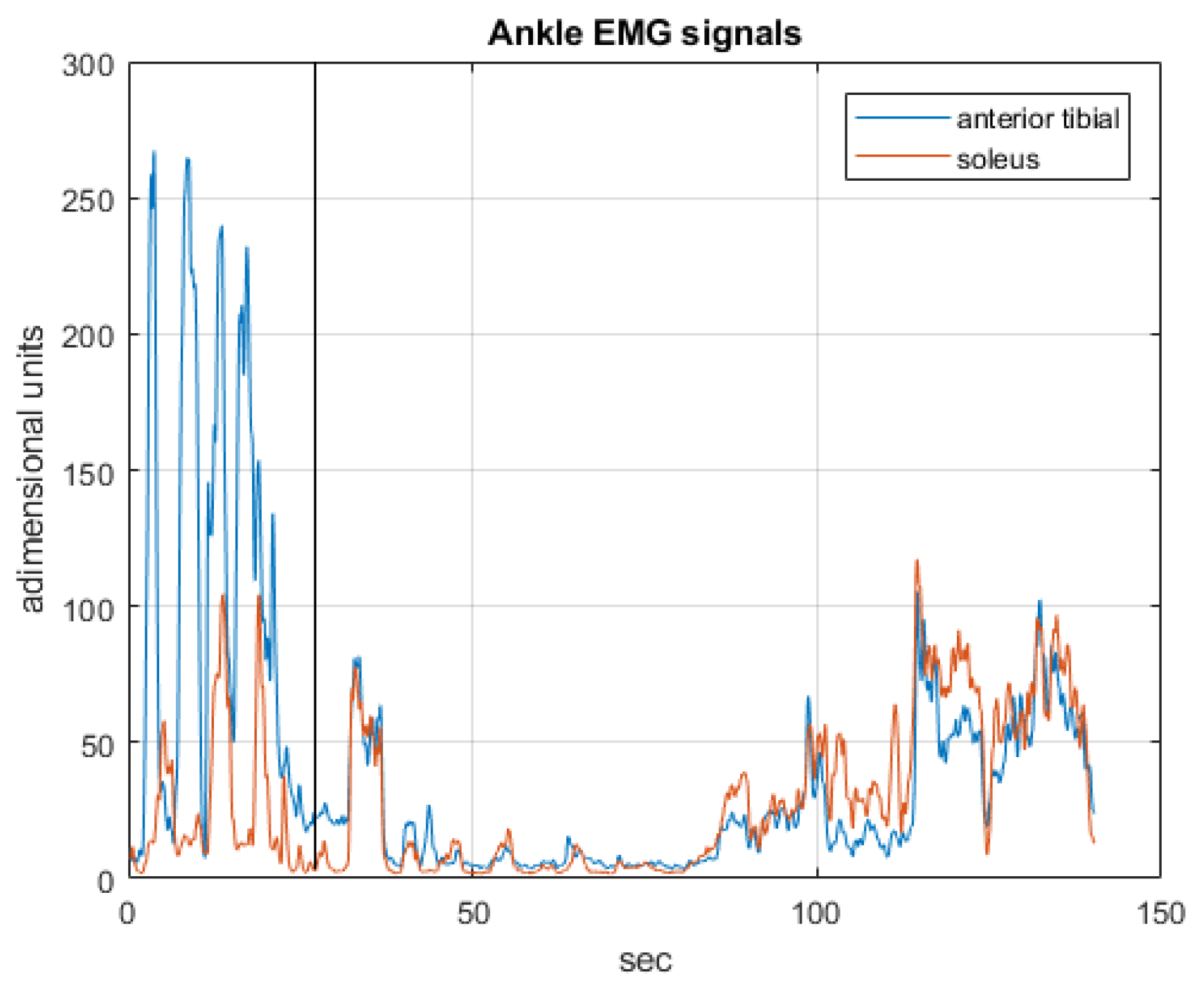
- for the ankle the two antagonistic muscles of anterior tibial and soleus;
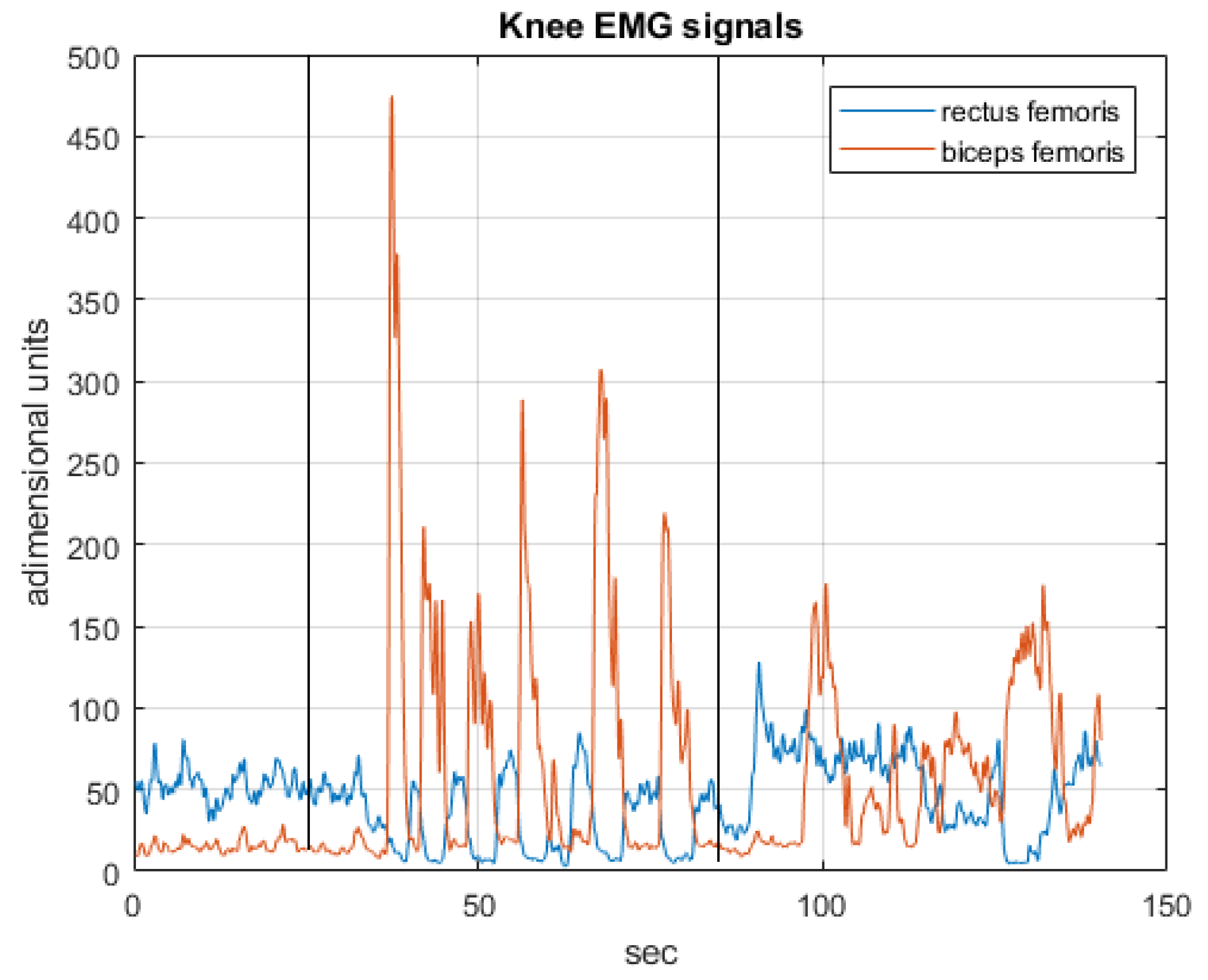
- for the knee Rectus femoris and Biceps femoris;
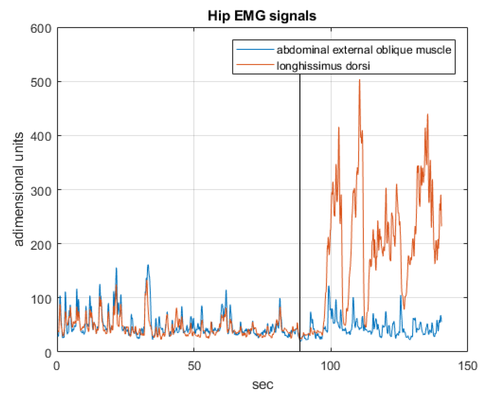
- for the hip abdominal external oblique muscle or alternatively Biceps femoris again and longhissimus dorsi or alternatively gluteus muscle.
The resulting EMG signals at the pair of antagonist muscles for each joint are processed as in Section 4.1. Moreover, attitude sensors are available on the trunk, approximatively at the center of mass of the patient.
The patient, sitting on a bicycle-like saddle at the hips level, and with legs and feet bound to the exoskeleton, is allowed three degrees of freedom, following three postural exercises:
- maintaining the equilibrium in the sagittal plane, i.e., moving longitudinally along the feet soles the COP;
- raising or lowering the trunk;
- changing the attitude of the trunk.
Each joint (pairs of ankles, knees and hips) is automatically controlled through the measures of the COP, the inertial sensors, and the speed/position of the joints, or by the patient, driven by EMG signals, and these controls can be inter-mixed [51].
4.2.3. Experiment Results
In the experiments documented here, the patient is allowed to control one degree of freedom at a time, leaving the remaining two to the automatic control. Hence, three experiments were performed:
- The patient controls the ankle (equilibrium), moving the COP forward and backward under the sole of the feet, while the height (or the knee angle) and attitude of the trunk is automatically maintained.
- The patient controls the knees raising and lowering the trunk, and the automatic control guarantees equilibrium and trunk attitude.
- The patient controls the hip angle changing the trunk attitude, while equilibrium and trunk height (knee angles) are guaranteed by the automatic control.
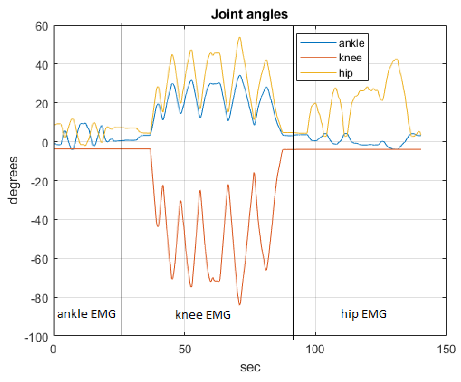
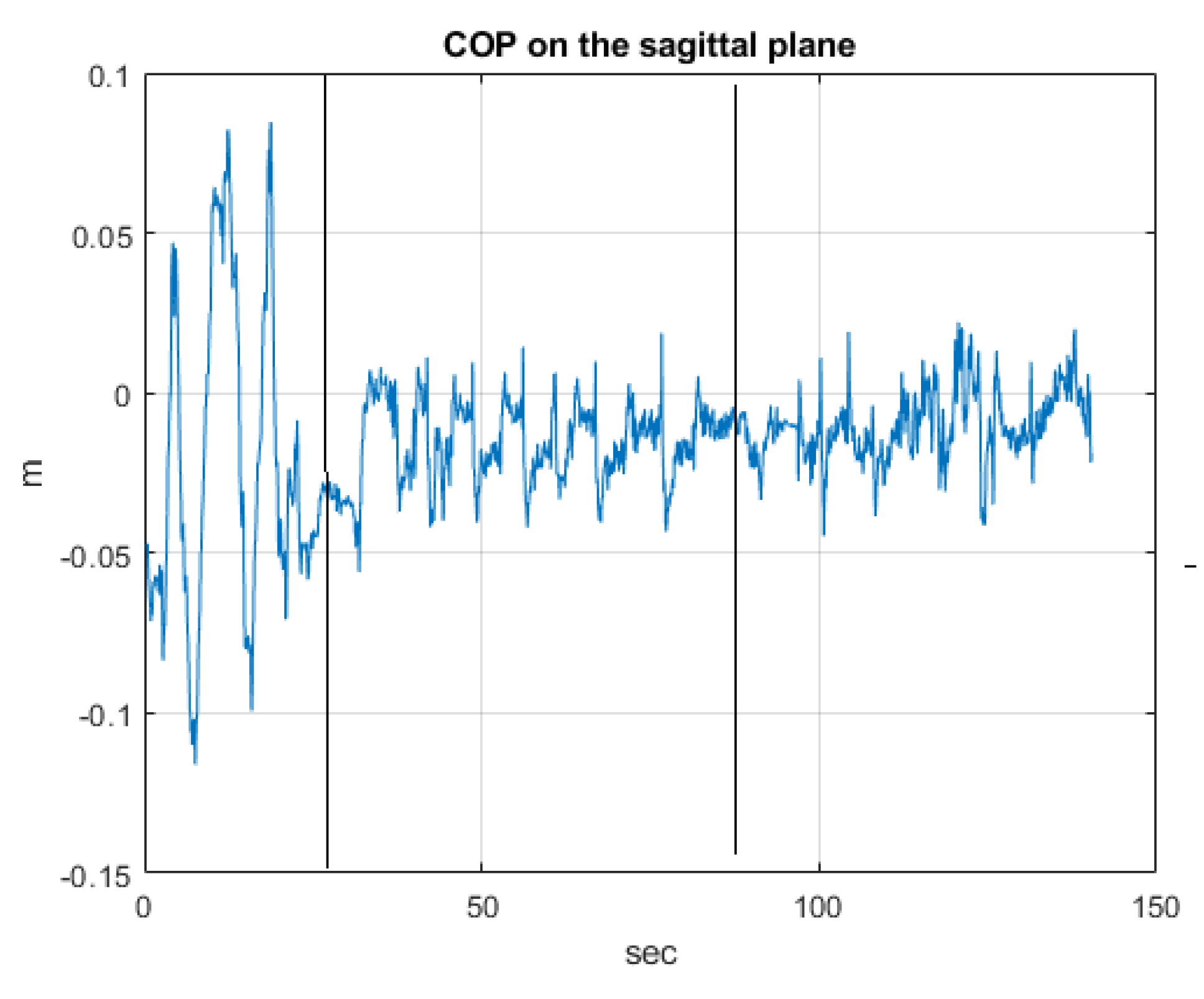
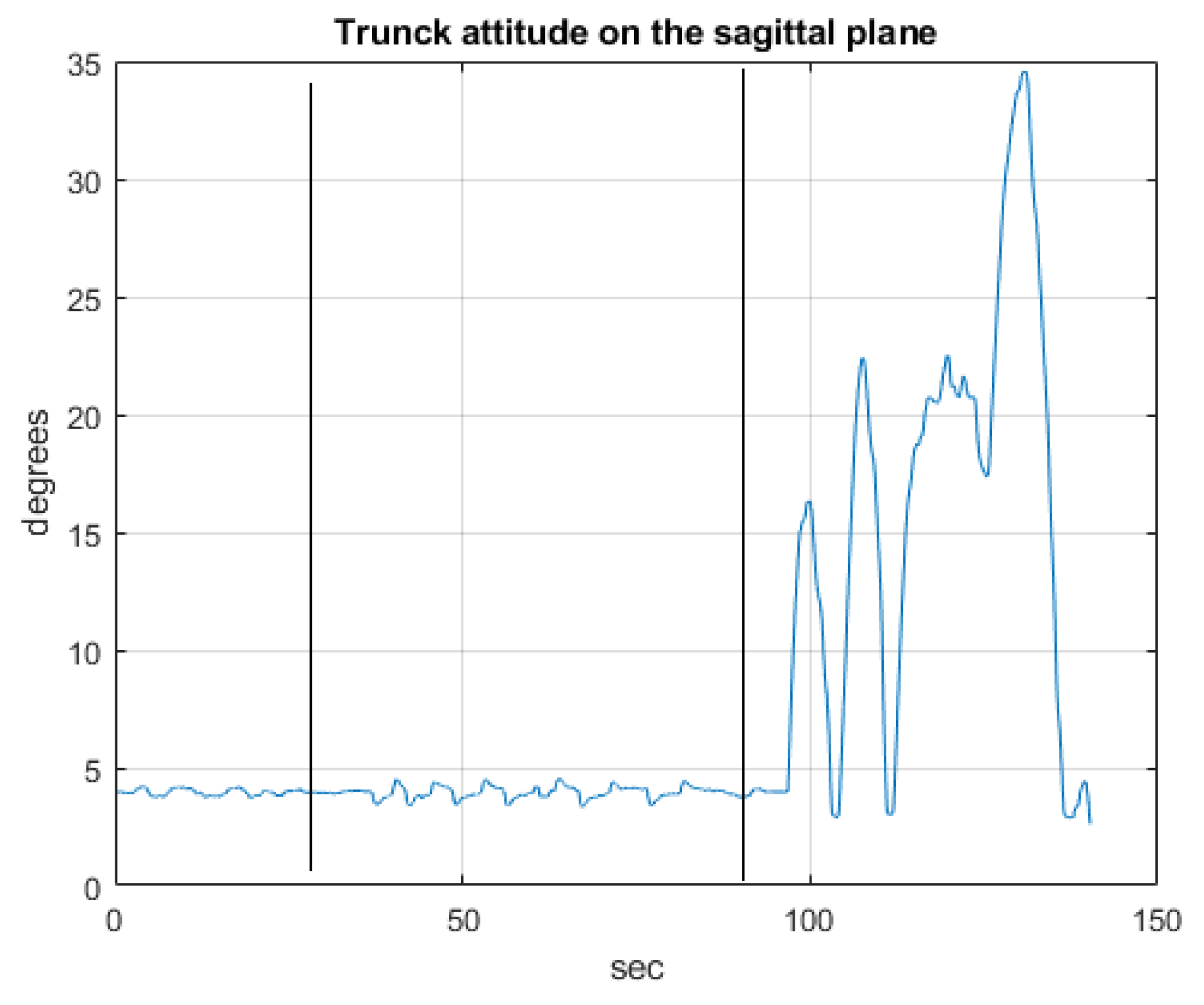
Experiments have been performed on healthy patients, regulating the admittance of the controlled joint to guarantee a comfortable compliance. Figure 15, Figure 16 and Figure 17 show the joint angles, the COP and trunk attitude behavior. In the first 30 s the patient controls the ankle (knees and trunk attitude are automatically maintained), from 30 to 90 s controls the knees (COP and trunk attitude are automatically maintained), and from 90 s to the end controls the hips (COP and knee angles are automatically maintained), performing a sequence of alternating motions.
4.3. Simulated Case Studies
In this section, results based on the simulation of a realistic case study of a 75 kg patient, 1.75 m tall, wearing a 45 kg exoskeleton are shown. The model has been dimensioned using standard anthropometric data [52]. The height of the barycenter is m, relatively low due to the weight of the exoskeleton, the distance between the center points of the two feet is m along y axis.
In single stance the equilibrium region is in the range of the foot length m] along the x axis (sagittal plane), and width m] along the y axis (frontal plane), with respect to the center foot coordinates , . Instead, in double stance this region is in the range of the two feet, m] along the y axis with respect to the ground projection of the center pelvis in the upright position.
Simulation of the non-linear switching dynamics of the 3D system assuming the patient bound to the exoskeleton, as described in [41], in closed loop control was performed. Characteristics of the compliance loop, designed from the linearized model of the system, are those shown in Figure 6. The steady state gain of for each joint is assumed to be 1 [rad/Nm], which means high compliance. Gains of the postural control loop were set at , and .
The following exercises were simulated:
- Sit-to-stand in double stance (motion in the sagittal plane);
- Reaching the limits and standing in equilibrium on one foot (motion in sagittal andl frontal planes);
- Step machine exercise (motion in sagittal and frontal planes).
The reference exoskeleton position for linearization was the standing up posture with slightly bent knees. In all the exercises the feedforward input of the control, i.e., the results of the EMG signals from the patient, were all simulated, and the same exercise was repeated twice: the first time the patient was approximatively able to move all joints in a coordinated way so as to spontaneously maintain equilibrium, while the second time, because of illness or weakness, disturbances which may compromise postural equilibrium were introduced. When not specified differently, the angles induced by the disturbances of the patient were of the order of approximately [rad]. Note that those disturbances were applied to the simulated patient signal, and hence may represent either a signal disturbance, or a patient’s incorrect movement.
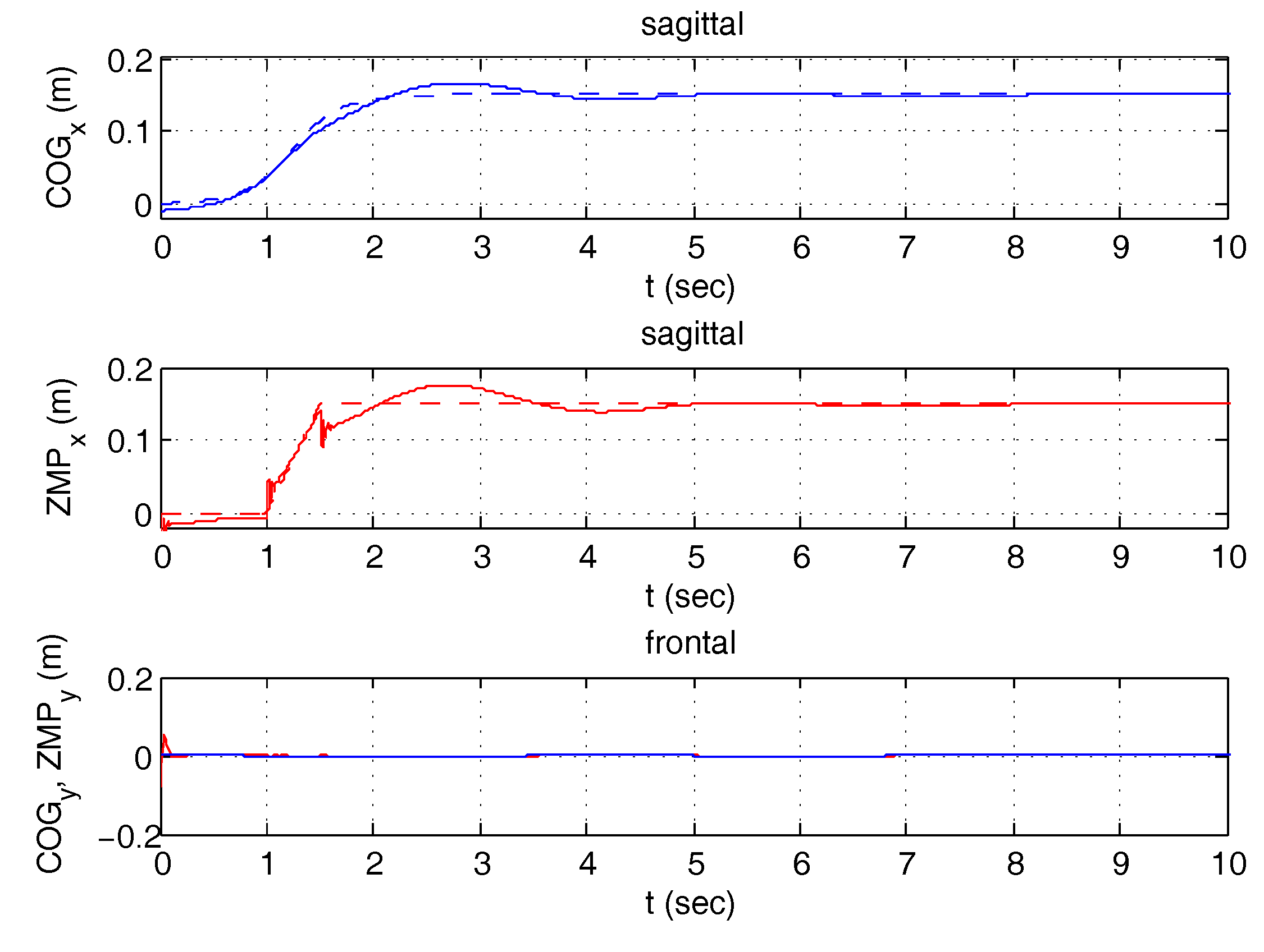
4.3.1. Sit to Stand Exercise
This exercise was performed in double stance balancing the weight equally on the two feet. The patient executed a coordinated transition -stand-to-sit-to-stand- (in reality without reaching the chair) controlling ankles, knees and hips: the action caused the joints to perform an approximate bell function: where is a bell function lasting 5 s with maximum value of . Simultaneously, while the control maintains central posture on the frontal plane, a preview control on the sagittal plane forced the patient to transfer the to his toes. Figure 21 shows and trajectories in sagittal and frontal planes with their preview reference values (dashed lines) when the patient behaved in a coordinated way.
The upper figures in Figure 22 refers to the same exercise when the patient lost control of knee 1, simulated by generating an angle that is half that of the other knee (). Disabling postural control on the sagittal plane, the patient lost postural equilibrium completely after a few seconds ( exits from the postural limit of m). Enabling postural control, the effects of the incorrect action is almost negligible. In this case, the frontal posture (not shown) was maintained in the central position by the control. The lower figures in Figure 22 represent the simulation of the same exercise when a sinusoidal disturbance, influencing posture on the frontal plane, is introduced on the simulated EMG signal controlling , disabling or enabling postural control on the frontal plane.
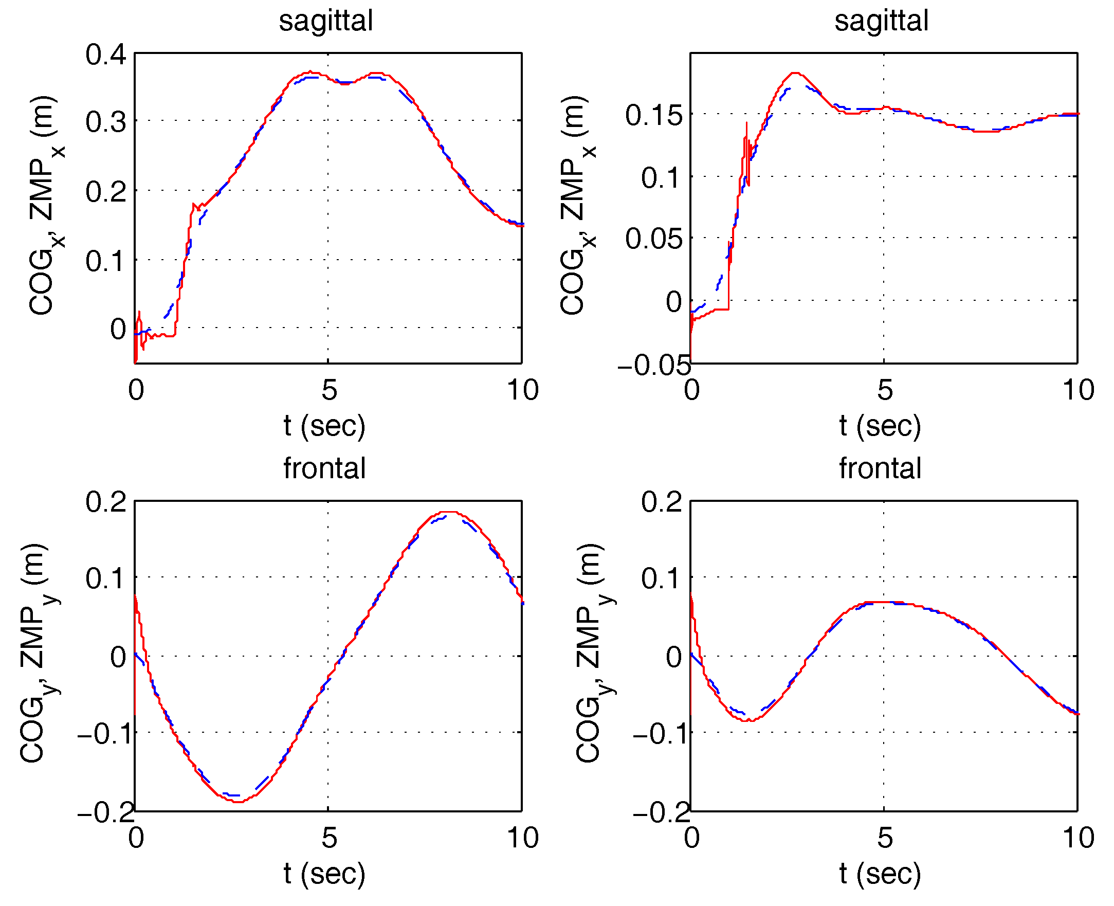
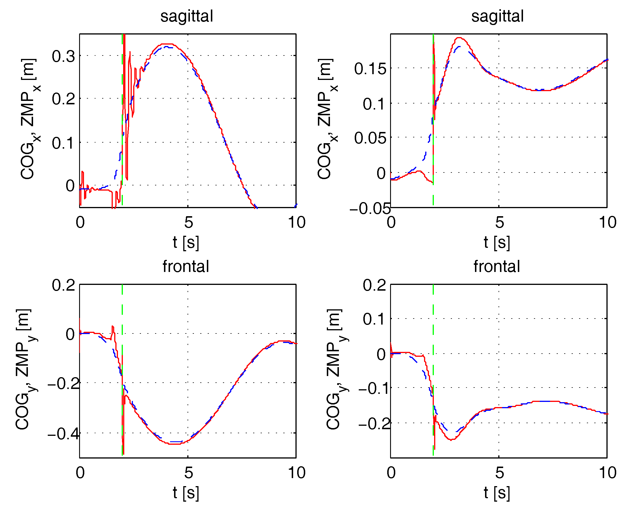
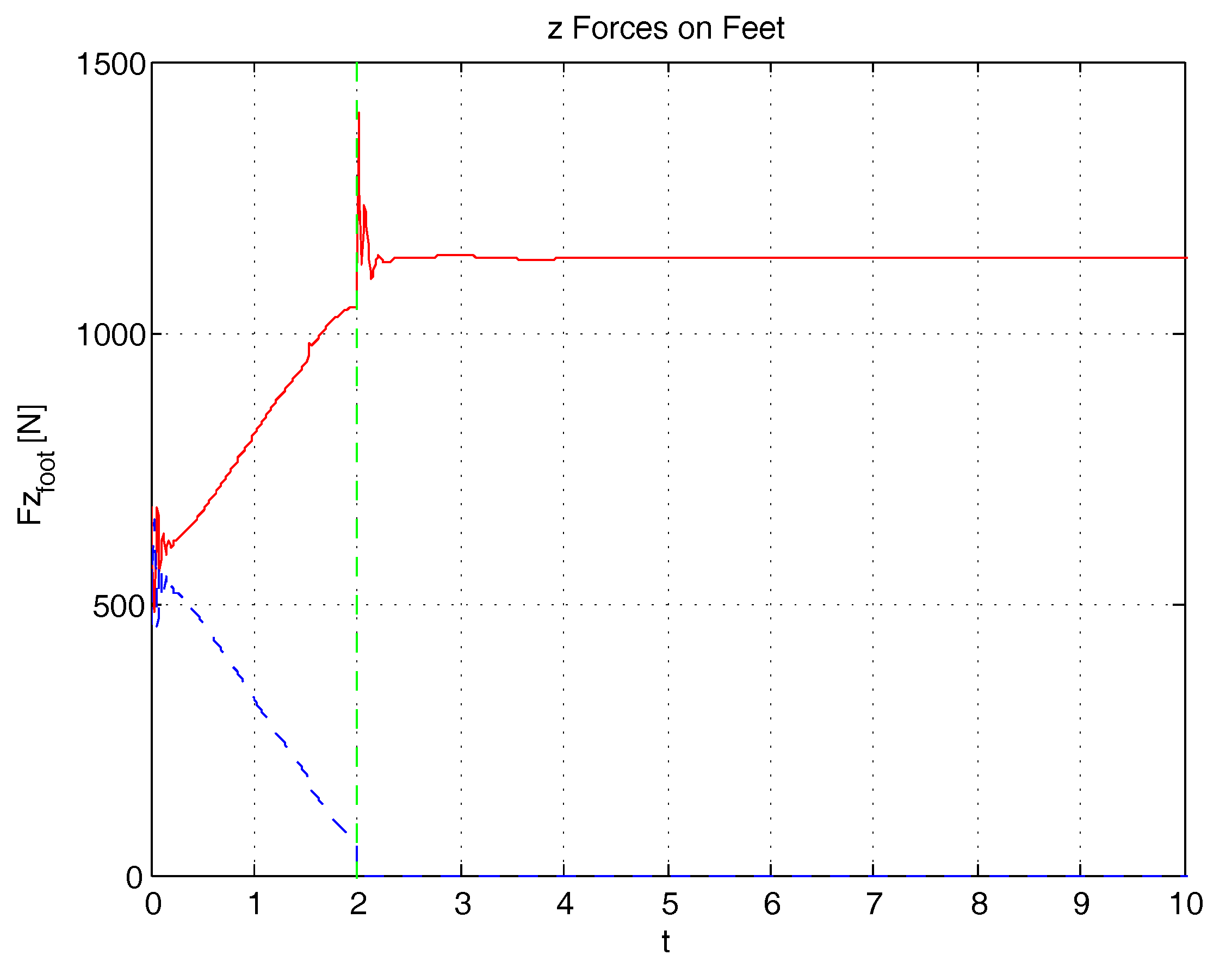
4.3.2. Reaching the Limits of Equilibrium
The exercise consists of one single step starting from a central balanced position: the in the frontal plane is transferred to the right foot, while in the sagittal plane it moves from the center to the toe. The system switches to single stance (a vertical dashed line is shown in all the figures when a change in stance happens) and the patient raises the free foot. In the first case, the patient behaves as expected. Simulation results for - and - coordinates are presented in Figure 23. In the second case, the patient has a disturbance on both signals that control and of the supporting ankle causing an error of about rad. Figure 24 shows how the exoskeleton behaves when sagittal control is deactivated/activated (first row) and when frontal control is deactivated/activated (second row). Again, the exoskeleton is able to reduce the effect of the incorrect movements by the patient, and keeps the on a stable trajectory. In Figure 25, the vertical forces below the feet are plotted, showing the results of the reaction force control described in Section 3.2.5. Observe that the exoskeleton starts from a balanced position and then all the weight is moved to the supporting foot.
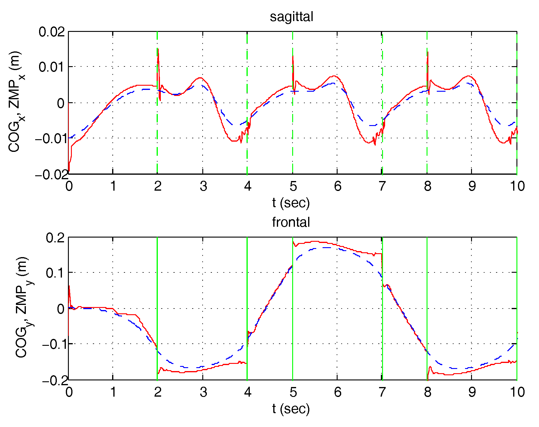
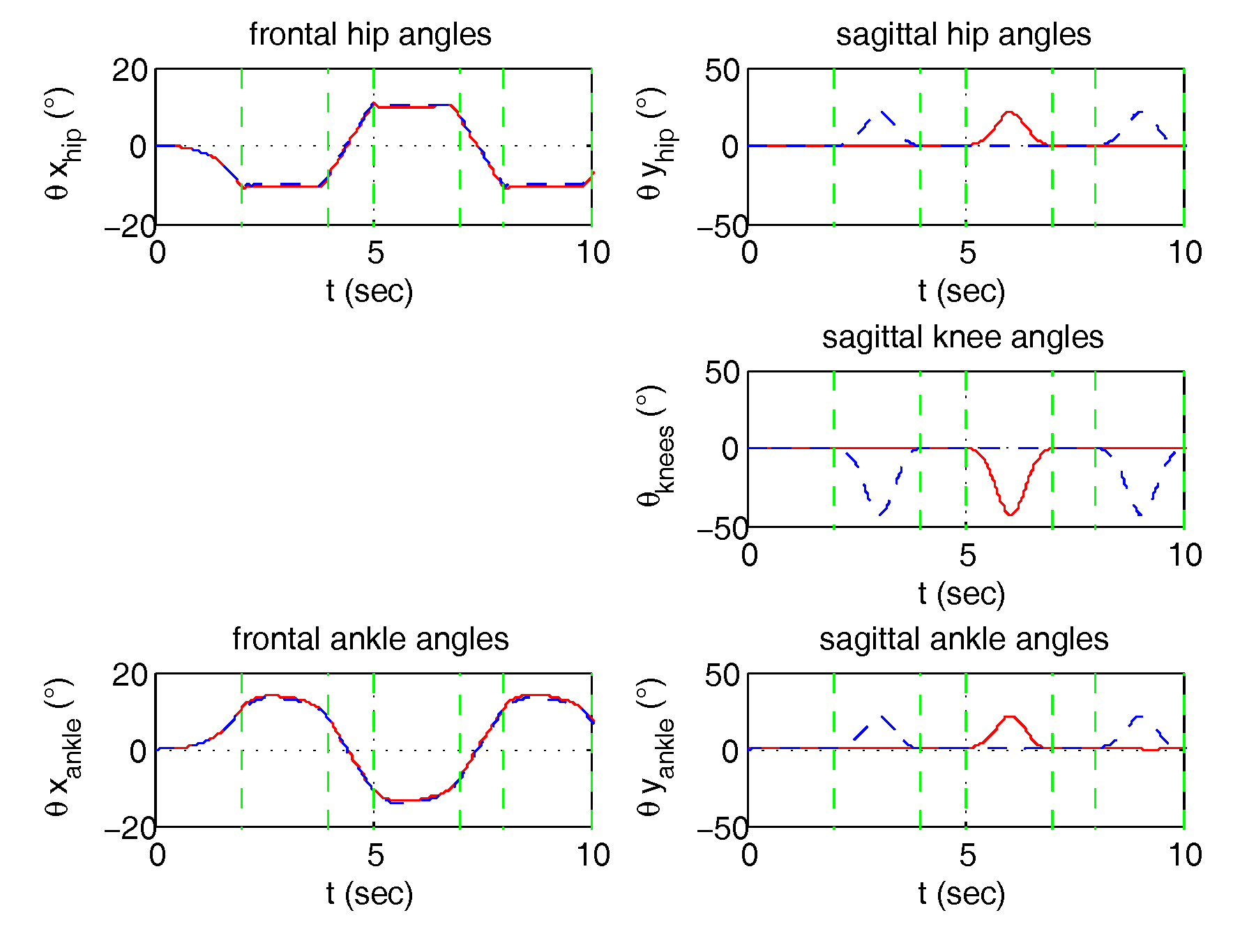
4.3.3. Step Machine Exercise
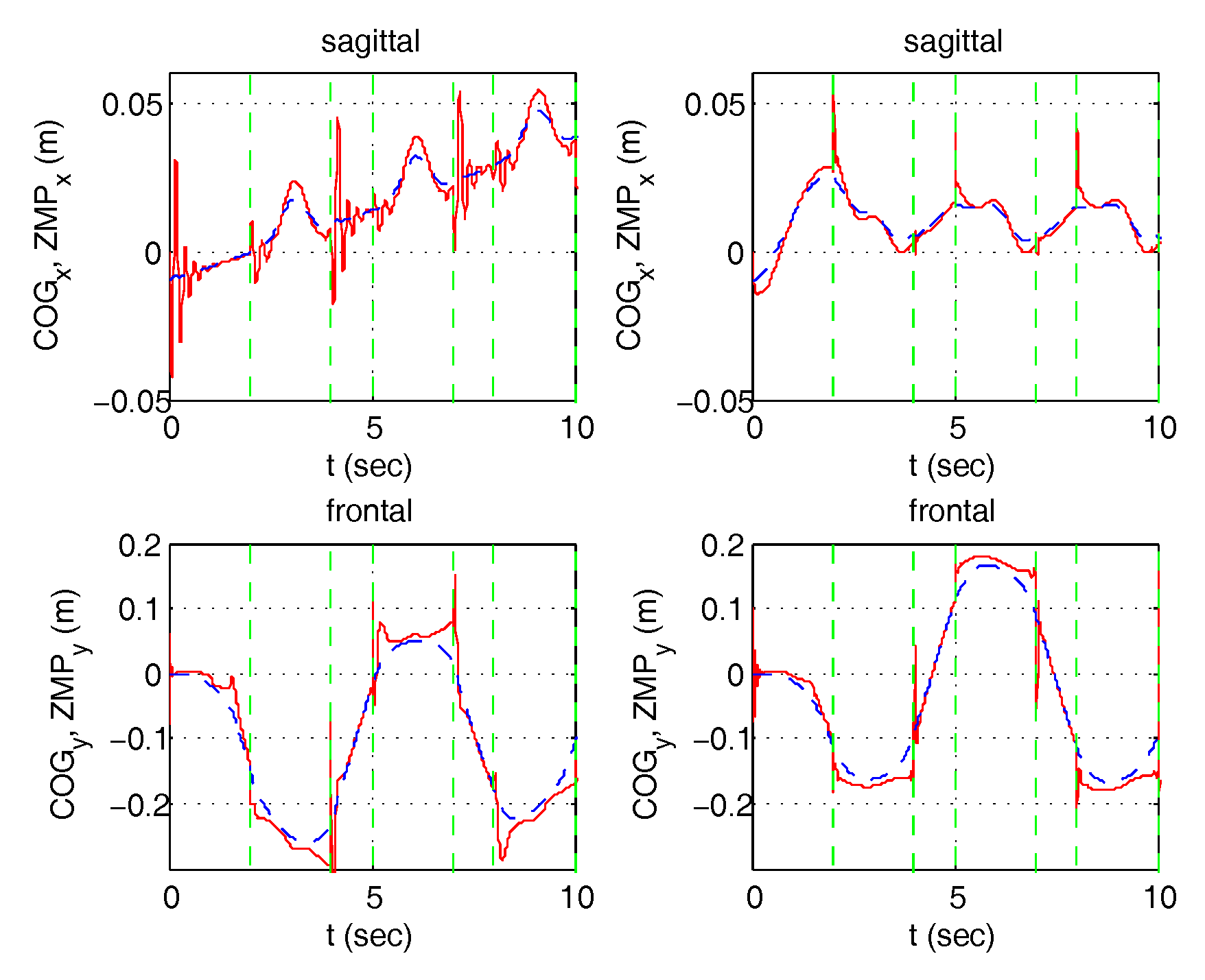
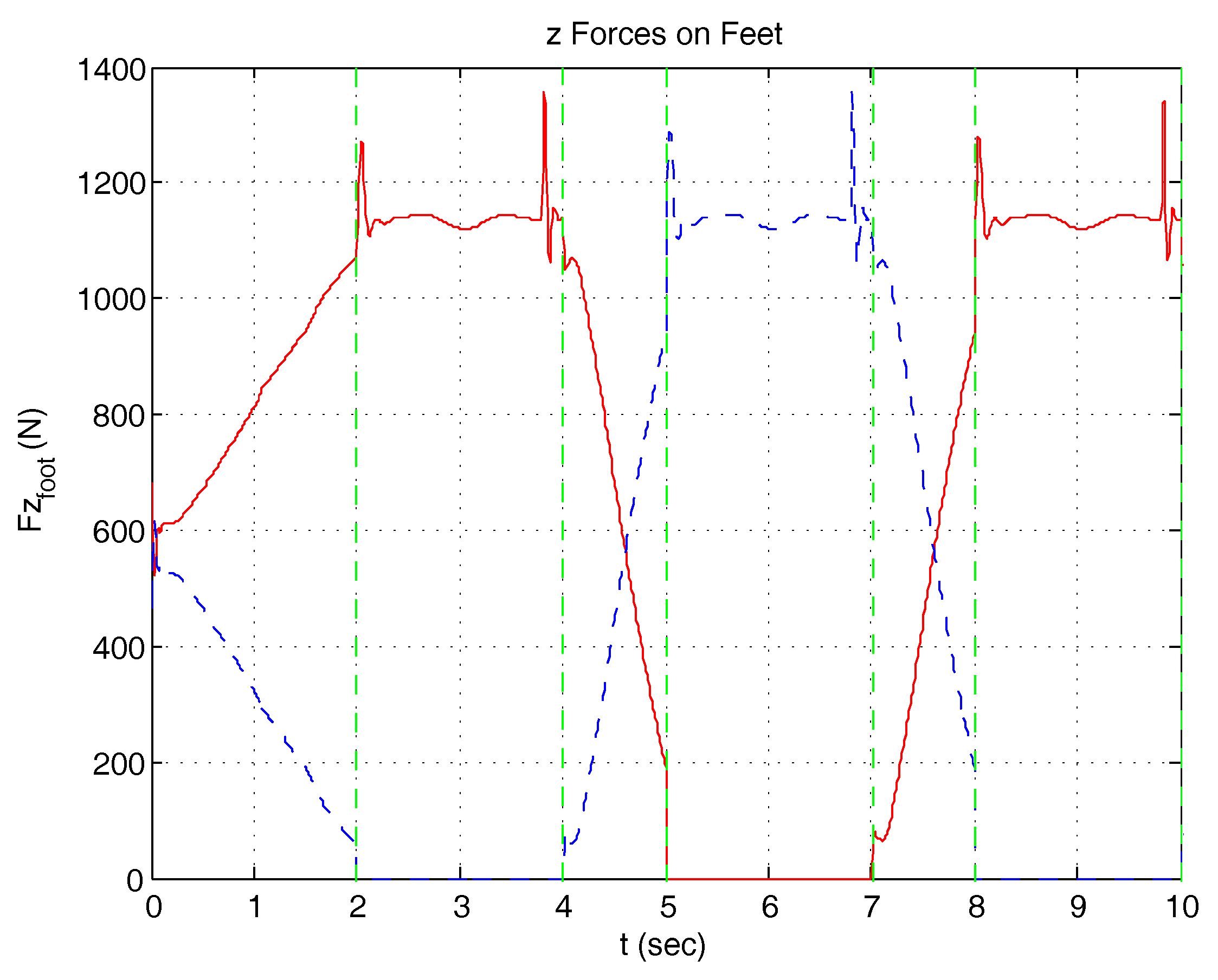
The step machine exercise emulates gait on a fixed position. The exercise requires the weight to be transferred alternatively between the left and the right foot with the help of the control. When the patient is balanced on a single foot, the control switches to single stance and with coordination the patient is able to raise the free foot, controlling his ankle, knee and hip joints. A preview control is generated for the frontal plane, achieved by completing, at the beginning and at the end, the periodic behavior proposed by Choi [39] with two aperiodic steps, starting and terminating on the center balance. The sagittal posture is maintained in an erect position simply by exploiting the extended Jacobian of Equation (12). The weight transfer in double stance was enabled. Figure 26 and Figure 27 refer to the results when postural control is active and no disturbances are induced by the patient and represents the /x and y coordinates and the joint angles. Disturbances originated in the patient signals (in this case ramp functions) causes a perturbation on and . The behavior of the system is simulated with enabled or disabled postural control (Figure 28). Vertical reaction forces, showing how the weight is transferred from one foot to another, are shown in Figure 29. Finally, frontal and sagittal foot reaction forces are presented in Figure 30.
5. Conclusions
In this paper, an haptic exoskeleton for rehabilitation, integrating patient compliance and postural equilibrium control is proposed, to our knowledge for the first time. The patient is able to move the exoskeleton joints through signals from the leg muscles, experiencing an admittance reaction from the position imposed by the automatic control of postural equilibrium. This has been achieved with two hierarchical closed loops: the internal one on the joint space for admittance control in a position loop, and the outer one on the Cartesian space for postural equilibrium. The advantages with respect to previous approaches, based on impedance or force control, is that it fully exploits the power of position feedback. Once a control loop robustly stabilises a non-linear system with proper loop frequency bandwidth, nonlinearity effects and the sensitivity on both parameter uncertainty and unknown disturbances, including unwanted patient movements, are greatly reduced. The unreliable inverse dynamics to evaluate patient torques or even gravity contributions is no longer needed to move the joints. Vice versa it can be naturally obtained by the feedback. Even if stability of the non-liner system in all possible configurations cannot be mathematically proved, adoption of a approach in the inner loop, and the inverted pendulum approximation, as proposed by Choi for the outer one, show a great robustness in all simulation experiments.
Theory shows that if the desired admittance in the two degrees of freedom control design is changed, the patient’s compliance can easily be modified according to the choice of the physiologist and the progresses of the rehabilitation. The practical achievable limits of compliance/bandwidth are dictated only by the level of noise actually present in the signals. This is currently the object of further investigation. Moreover, postural control is able to accommodate incorrect actions by the patient. In this respect, a further object of experiments is the interaction of the unwanted feedback loop generated by the patient’s physiology and the exoskeleton postural control. The use of the pseudo-inverse of the Jacobian has been limited here to the control of the and non interactively. However, extensions, exploiting the same idea, can easily be considered for the motion of other parts of the multi-chain, e.g., trunk attitude, , free foot position or trajectory, etc., with full interaction on both planes.
6. Patents
Author Contributions
G. Menga and M. Ghirardi conceived and designed the experiments; G. Menga performed the experiments on the prototypes; M. Ghirardi performed the simulated experiments; G. Menga and M. Ghirardi wrote the paper.
Acknowledgments
This research has been partially supported by MIUR the Italian Ministry of Instruction, University and Research and the Piedmont Region.
Conflicts of Interest
The authors declare no conflict of interest.
References
- Vukobratovic, M. Humanoids Robots: Past, Present State, Future. In Proceedings of the 4th SISY—Serbian-Hungarian Joint Symposium on Intelligent Systems, Subotica, Serbia, 29–30 September 2006. [Google Scholar]
- Dollar, A. Lower Extremity Exoskeletons and Active Orthoses: Challenges and State-of-the-Art. IEEE Trans. Robot. 2008, 24, 144–158. [Google Scholar] [CrossRef] [Green Version]
- Fleischer, C.; Wege, A.; Kondak, K.; Hommel, G. Controlling Exoskeletons with EMG Signals and a Biomechanical Body Model. Ph.D. Thesis, Fakultat IV—Elektrotechnik und Informatik Technische Universitat Berlin, Berlin, Germany, 2007. [Google Scholar]
- Kleim, J.; Jones, T. Principles of Experience-Dependent Neural Plasticity: Implications for Rehabilitation After Brain Damage. J. Speech Lang. Hear. Res. 2008, 51, 225–239. [Google Scholar] [CrossRef]
- Agrawal, S.K.; Banala, S.K.; Fattah, A.; Sangwan, V.; Krishnamoorthy, V.; Scholz, J.P.; Hsu, W.L. Assessment of Motion of a Swing Leg and Gait Rehabilitation With a Gravity Balancing Exoskeleton. IEEE Trans. Neural Syst. Rehabil. Eng. 2007, 15, 410–420. [Google Scholar] [CrossRef] [PubMed] [Green Version]
- Tansey, K. The Use of the Lokomat System in Clinical Research. In Proceedings of the 2009 International Neurorehabilitation Symposium, Zurich, Switzerland, 12–13 February 2009. [Google Scholar]
- Duschau-Wicke, A.; von Zitzewitz, J.; Caprez, A.; Lünenburger, L.; Riener, R. Path Control: A Method for Patient-Cooperative Robot-Aided Gait Rehabilitation. IEEE Trans. Neural Syst. Rehabil. Eng. 2010, 18, 38–48. [Google Scholar] [CrossRef] [PubMed] [Green Version]
- Banala, S.K.; Kim, S.H.; Agrawal, S.K.; Scholz, J.P. Robot Assisted Gait Training With Active Leg Exoskeleton (ALEX). IEEE Trans. Neural Syst. Rehabil. Eng. 2009, 17, 2–8. [Google Scholar] [CrossRef] [PubMed]
- Vukobratovic, M.; Borovac, B.; Surla, D.; Stokic, D. Biped Locomotion: Dynamics, Stability, Control, and Application; Springer: Berlin/Heidelberg, Germany, 1990. [Google Scholar]
- Kajita, S.; Espiau, B. Legged Robots. In Springer Handbook of Robotics; Springer: Berlin/Heidelberg, Germany, 2008; pp. 361–389. [Google Scholar]
- Zoss, A.; Kazerooni, H.; Chu, A. Biomechanical Design of the Berkeley Lower Extremity Exoskeleton (BLEEX). IEEE/ASME Trans. Mechatron. 2006, 11, 128–138. [Google Scholar] [CrossRef]
- Kazerooni, H.; Huang, L.; Steger, R. On the Control of the Berkeley Lower Extremity Exoskeleton (BLEEX). In Proceedings of the 2005 IEEE International Conference on Robotics and Automation, Barcelona, Spain, 18–22 April 2005. [Google Scholar]
- Pratt, J.; Krupp, B.; Morse, C.; Collins, S. The RoboKnee: An Exoskeleton for Enhancing Strength and Endurance During Walking. In Proceedings of the 2004 IEEE International Conference on Robotics and Automation, New Orleans, LA, USA, 1–26 April 2004. [Google Scholar]
- Kawamoto, H.; Suwoong, L.; Kanbe, S.; Sankai, Y. Power Assist Method for HAL-3 Using EMG-based Feedback Controller. In Proceedings of the 2004 IEEE International Conference on Systems, Man and Cybernetics, The Hague, The Netherlands, 10–13 October 2004. [Google Scholar]
- Kasaoka, K.; Sankai, Y. Predictive Control Estimating Operators Intention for Stepping-up Motion by Exoskeleton Type Power Assist System HAL. In Proceedings of the IEEE/RSI International Conference on Intelligent Robots and Systems, Maui, HI, USA, 29 October–3 November 2001. [Google Scholar]
- Kawamoto, H.; Sankai, Y. Comfortable Power Assist Control Method for Walking Aid by HAL-3. In Proceedings of the IEEE International Conference on System, Man and Cjbernetics, Yasmine Hammamet, Tunisia, 6–9 October 2002. [Google Scholar]
- Lee, S.; Sankai, Y. Power Assist Control method for walking aid by HAL-3 Based on EMG and Impedance Adjustment around Knee Joint. In Proceedings of the 2002 IEEE/RSJ Conference on Intelligent Robots and Systems, Lausanne, Switzerland, 30 September–4 October 2002. [Google Scholar]
- Fleischer, C.; Wege, A.; Kondak, K.; Hommel, G. Application of EMG Signals for Controlling Exoskeleton Robots. Biomed. Tech. 2006, 51, 314–319. [Google Scholar] [CrossRef] [PubMed]
- Yamamoto, K.; Ishii, M.; Noborisaka, H.; Hyodo, K. Stand Alone Wearable Power Assisting Suit-Sensing and Control Systems. In Proceedings of the IEEE International Workshop on Robot and Human Interactive Communication, Okayama, Japan, 20–22 September 2004. [Google Scholar]
- Viteckova, S.; Kutilek, P.; Jirina, M. Wearable lower limb robotics: A review. Biocybern. Biomed. Eng. 2013, 33, 96–105. [Google Scholar] [CrossRef]
- Holanda, L.J.; Silva, P.M.M.; Amorim, T.C.; Lacerda, M.O.; Simao, C.R.; Morya, E. Robotic assisted gait as a tool for rehabilitation of individuals with spinal cord injury: A systematic review. J. Neuroeng. Rehabil. 2017, 14, 126. [Google Scholar] [CrossRef] [PubMed]
- Morone, G.; Paolucci, S.; Cherubini, A.; Angelis, D.D.; Venturiero, V.; Coiro, P.; Iosa, M. Robot-assisted gait training for stroke patients: current state of the art and perspectives of robotics. Neuropsychiatr. Dis. Treat. 2017, 13, 1303–1311. [Google Scholar] [CrossRef] [PubMed]
- Esquenazi, A.; Talaty, M.; Jayaraman, A. Powered Exoskeletons for Walking Assistance in Persons with Central Nervous System Injuries: A Narrative Review. PM R 2017, 9, 46–62. [Google Scholar] [CrossRef] [PubMed]
- Calabro, R.S.; Cacciola, A.; Berte, F.; Manuli, A.; Leo, A.; Bramanti, A.; Naro, A.; Milardi, D.; Bramanti, P. Robotic gait rehabilitation and substitution devices in neurological disorders: Where are we now? Neurol Sci. 2016, 37, 503–514. [Google Scholar] [CrossRef] [PubMed]
- Rex Bionics, Rex. 2010. Available online: www.rexbionics.com (accessed on 6 June 2018).
- Almesfer, F.; Grimmer, A.J. Control System for a Mobility Aid. European Patent EP2,448,540 A4, 1 July 2009. [Google Scholar]
- Menga, G. System for Controlling an Exoskeleton Haptic Device for Rehabilitation Purposes, and Corresponding Exoskeleton Haptic Device. European Patent EP2,238,894, 17 April 2009; U.S. Patent 8,556,836 B2, 7 April 2009. [Google Scholar]
- Kolakowsky-Hayner, S.; Crew, J.; Moran, S.; Shah, A. Safety and Feasibility of using the EksoTM Bionic Exoskeleton to Aid ambulation after spinal cord injury. J. Spine 2013. [Google Scholar] [CrossRef]
- Indego. Available online: http://www.indego.com/indego/en/home (accessed on 6 June 2018).
- Farris, R.J.; Quintero, H.A.; Goldfarb, M. Performance Evaluation of a Lower Limb Exoskeleton for Stair Ascent and Descent with Paraplegia. Conf. Proc. IEEE Eng. Med. Biol. Soc. 2012, 2012, 1908–1911. [Google Scholar] [PubMed]
- Esquenazi, A.; Talaty, M.; Packel, A.; Saulino, M. The ReWalk powered exoskeleton to restore ambulatory function to individuals with thoracic-level motor-complete spinal cord injury. Am. J. Phys. Med. Rehabil. 2012, 91, 911–921. [Google Scholar] [CrossRef] [PubMed]
- Mindwalker. Available online: https://mindwalker-project.eu/ (accessed on 6 June 2018).
- Adams, R.; Hannaford, B. Control Law Design for Haptic Interfaces to Virtual Reality. IEEE Trans. Control Syst. Technol. 2002, 10, 3–13. [Google Scholar] [CrossRef]
- Wen, K.; Necsulescu, D.; Sasiadek, J. Haptic Force Control Based on Impedance/Admittance Control Aided by Visual Feedback. Multimedia Tools Appl. J. 2008, 37, 39–52. [Google Scholar] [CrossRef]
- Menga, G.; Ghirardi, M. Modeling, Simulation and Control of the Walking of Biped Robotic Devices, Part II: Rectilinear Walking. Inventions 2016, 1, 7. [Google Scholar] [CrossRef]
- Vukobratovic, M.; Borovac, B. Zero-Moment-Point - Thirty Five Years of Its Life. Int. J. Humanoid Robot. 2004, 1, 157–173. [Google Scholar] [CrossRef]
- Siciliano, B.; Khatib, O. (Eds.) Springer Handbook of Robotics; Springer: Berlin/Heidelberg, Germany, 2008; Chapter 16. [Google Scholar]
- Kim, J.H.; Han, J.W.; Kim, D.Y.; Baek, Y.S. Design of a Walking Assistance Lower Limb Exoskeleton for Paraplegic Patients and Hardware Validation Using CoP. Int. J. Adv. Robot. Syst. 2013, 10, 1–7. [Google Scholar] [CrossRef]
- Choi, Y.; Kim, D.; Oh, Y.; You, B. Posture/Walking Control for Humanoid Robot Based on Kinematic Resolution of CoM Jacobian With Embedded Motion. IEEE Trans. Robot. 2007, 23, 1285–1293. [Google Scholar] [CrossRef]
- Kane, T.; Levinson, D. Dynamics: Theory and Applications; McGraw-Hill: New York, NY, USA, 1985. [Google Scholar]
- Menga, G.; Ghirardi, M. Modelling, Simulation and Control of the Walking of Biped Robotic Devices—Part I: Modelling and Simulation Using Autolev. Inventions 2016, 1, 6. [Google Scholar] [CrossRef]
- Mitiguy, P. MotionGenesis: Advanced Solutions for Forces, Motion, and Code-Generation. 2000. Available online: http://www.motiongenesis.com/ (accessed on 6 June 2018).
- Ueberle, M.; Buss, M. Control of Kinesthetic Haptic Interfaces. In Proceedings of the IEEE/RSJ International Conference on Intelligent Robots and Systems (IROS 2004), Sendai, Japan, 28 September–2 October 2004. [Google Scholar]
- Carignan, C.; Cleary, K. Closed-Loop Force Control for Haptic Simulation of Virtual Environments. Haptics-e 2000, 1. [Google Scholar]
- Horowitz, M. Synthesis of Feedback Systems; Academic Press: New York, NY, USA, 1963. [Google Scholar]
- Doyle, J.; Stein, G. Multivariable Feedback Design: Concepts for a Classical/Modern Synthesis. IEEE Trans. Autom. Control 1991, 26, 4–16. [Google Scholar] [CrossRef]
- Zhou, K.; Doyle, J.; Glover, K. Robust and Optimal Control; Prentice Hall: Upper Saddle River, NJ, USA, 1996. [Google Scholar]
- Colaneri, P.; Locatelli, J.G. Control Theory and Design. A RH2-RHinf Viewpoint; Academic Press: New York, NY, USA, 1997. [Google Scholar]
- Kajita, S.; Kanehiro, F.; Kaneko, K.; Fujiwara, K.; Harada, K.; Yokoi, K.; Hirukawa, H. Biped Walking Pat-tern Generation by using Preview Control of Zero-Moment Point. In Proceedings of the 2003 IEEE International Conference on Robotics and Automation, Taipei, Taiwan, 14–19 September 2003. [Google Scholar]
- Menga, G.; Ghirardi, M. Control of the sit-to-stand transfer of a biped robotic device for postural rehabilitation. Internal Report—Politecnico di Torino, Italy. Available online: https://www.dropbox.com/s/hfju6io2ht4b7o1/3.SITTOSTAND.pdf (accessed on 6 June 2018).
- Menga, G.; Ghirardi, M. Estimation and closed loop control of COG/ZMP in biped devices blending CoP measures and kinematic information. In Internal Report—Politecnico di Torino, Italy. Available online: https://www.dropbox.com/s/ombhavtvh99siwo/2.COGZMP.pdf (accessed on 6 June 2018).
- Winter, D. Biomechanics and Motor Control of Human Movement; John Wiley & Sons: Hoboken, NJ, USA, 2009. [Google Scholar]
- Menga, G. System for Controlling a Robotic Device During Walking, and Corresponding Robotic Device. European Patent EP2,497,610 A1, 9 March 2011. [Google Scholar]
- Menga, G. G++ Control, SYCO. 2009. Available online: http://www.syco.it/temp/controldesign3.zip, http://www.syco.it/temp/controlbook.zip (accessed on 6 June 2018).
Figure 1.
The exoskeleton.

Figure 2.
The exoskeleton: frontal and sagittal planes.

Figure 3.
Two Degrees of freedom control.

Figure 4.
The extended system-closed loop and specific for a two degrees of freedom design.

Figure 5.
Detailed Extended System.

Figure 6.
(left) Closed loop output sensitivity functions and (right) admittances, desired and achieved.
Figure 6.
(left) Closed loop output sensitivity functions and (right) admittances, desired and achieved.

Figure 7.
(left) sagittal plane (dashed) and in the extreme of equilibrium exercise and (right) Frontal plane (dashed) and in the step machine exercise.
Figure 7.
(left) sagittal plane (dashed) and in the extreme of equilibrium exercise and (right) Frontal plane (dashed) and in the step machine exercise.

Figure 8.
The postural control loop—one for each plane.

Figure 9.
Tracking of angle position and angular speed for high admittance.

Figure 10.
Tracking of angle position and angular speed for medium admittance.

Figure 11.
Tracking of angle position and angular speed for low admittance.

Figure 12.
EMG signals during one period of tracking for high, medium and low admittances.

Figure 13.
EMG signals comparison in isometric condition for different loads.

Figure 14.
The exoskeleton prototype.

Figure 15.
The joint angles.

Figure 16.
The COP behaviour.

Figure 17.
The trunk attitude.

Figure 18.
The EMG signals operating in the first phase.

Figure 19.
The EMG signals operating in the second phase.

Figure 20.
The EMG signals operating in the third phase.

Figure 21.
Sit to stand—Coordinate behavior.

Figure 22.
Sit to stand—in the presence of disturbances, without (left)/with (right) postural control enabled.
Figure 22.
Sit to stand—in the presence of disturbances, without (left)/with (right) postural control enabled.

Figure 23.
Reaching the limits of equilibrium—Coordinate behavior ZMP and COG (dashed).

Figure 24.
Reaching the limits of equilibrium—ZMP and COG (dashed)—in the presence of disturbances and without control (left)/with control (right).
Figure 24.
Reaching the limits of equilibrium—ZMP and COG (dashed)—in the presence of disturbances and without control (left)/with control (right).

Figure 25.
Reaching the limits of equilibrium—Vertical Forces on feet (dashed line = left leg).

Figure 26.
Step machine—Coordinate behavior ZMP and COG (dashed).

Figure 27.
Step Machine—Joint angles (dashed line = left leg).

Figure 28.
Step machine ZMP and COG (dashed)—in the presence of disturbances and without control (left)/with control (right).
Figure 28.
Step machine ZMP and COG (dashed)—in the presence of disturbances and without control (left)/with control (right).

Figure 29.
Step Machine: Vertical Forces on feet (dashed line = left leg).

Figure 30.
Step Machine: reaction forces/torques on feet (dashed line = left leg).

© 2018 by the authors. Licensee MDPI, Basel, Switzerland. This article is an open access article distributed under the terms and conditions of the Creative Commons Attribution (CC BY) license (http://creativecommons.org/licenses/by/4.0/).
Share and Cite
MDPI and ACS Style
Menga, G.; Ghirardi, M. Lower Limb Exoskeleton for Rehabilitation with Improved Postural Equilibrium. Robotics 2018, 7, 28. https://0-doi-org.brum.beds.ac.uk/10.3390/robotics7020028
AMA Style
Menga G, Ghirardi M. Lower Limb Exoskeleton for Rehabilitation with Improved Postural Equilibrium. Robotics. 2018; 7(2):28. https://0-doi-org.brum.beds.ac.uk/10.3390/robotics7020028
Chicago/Turabian StyleMenga, Giuseppe, and Marco Ghirardi. 2018. "Lower Limb Exoskeleton for Rehabilitation with Improved Postural Equilibrium" Robotics 7, no. 2: 28. https://0-doi-org.brum.beds.ac.uk/10.3390/robotics7020028
Note that from the first issue of 2016, this journal uses article numbers instead of page numbers. See further details here.