1. Introduction
On-site monitoring of crop growth throughout the growing season plays an important role in assessing overall crop conditions, determining when to irrigate, and forecasting potential yields [
1,
2,
3,
4]. Particularly, periodic monitoring of various biophysical properties of crops grown in a field, such as biomass, leaf area index, and plant height, can help growers to effectively optimize inputs such as fertilizers and herbicides as well as to accurately estimate final yields [
5,
6,
7]. Traditionally, crop-monitoring studies have used in-field measurements or airborne/satellite data to effectively cover wide areas. Field-based methods involving on-site sampling and laboratory analysis have disadvantages in collection of data because they are often destructive, labor-intensive, costly, and time consuming, thereby limiting the number of samples required for establishment of efficient crop growth management [
8,
9].
Precision agriculture is a site-specific soil and crop management system that assesses variability in soil properties (e.g., pH, organic matter, and soil nutrient levels) and field (e.g., slope and elevation) and crop parameters (e.g., yield and biomass) using various tools including the global positioning system (GPS), geographic information systems (GIS), and remote sensing (RS). To manage crops site -specifically, it is necessary to collect information such as crop and soil conditions and weed distribution at different locations in a field. Remote sensing of crops can be more attractive than traditional methods of crop monitoring due to the ability to cover large areas rapidly and repeatedly. Remote sensing techniques from manned airborne or satellite platforms have been widely adopted for crop monitoring [
3,
10] since measurements are non-destructive and non-invasive and enable scalable implementation in space and time [
11]. A common use of remote sensing is evaluation of crop growth status based on canopy greenness by quantifying the distribution of vegetation index (VI) in the crop field. Various vegetation indices, including Normalized Difference Vegetation Index (NDVI) and Excess Green (ExG), have been defined as representative reflectance values of the vegetation canopy [
12].
In recent years, unmanned aerial vehicles (UAVs) have been commonly used for low-altitude and high resolution-based remote sensing applications due to advantages such as versatility, light weight, and low operational costs [
2,
13]. In addition, UAVs offer a customizable aerial platform from which a variety of sensors can be mounted and flown to collect aerial imagery with much finer spatial and temporal resolutions compared to piloted aircraft or satellite remote sensing systems despite several limitations, such as relatively short flight time, lower payload, and the sensitivity to weather and terrain conditions. Advancements in the accuracy, economic efficiency, and miniaturization of many technologies, including GPS receivers and computer processors, have pushed UAV systems into a cost-effective, innovative remote sensing platform [
14]. Especially, multi rotor-based UAVs have been commonly used to assess the vegetation status of crops and predict their yields because the flexibility of vertical takeoff and landing platforms with various image sensors make it easy to fly over agricultural fields [
15]. The acquired aerial images can help farmers evaluate the status of crop growth such as canopy greenness, leaf area, water stress estimation, and various geographic conditions including crop area, digital surface models (DSMs), and depth contour lines [
16,
17].
Several review articles have highlighted the wide range of applications for UAVs and mounted sensors. In the area of agriculture, based on optical diffuse reflectance sensing in the visible and near-infrared (NIR) ranges studying the interaction between incident light and crop surface properties, UAVs have been adopted for monitoring of water status and drought stresses in fruit trees using NIR band data [
18]; additionally, they have been used for collecting multispectral and hyperspectral imagery for use in spectral indices [
19] and even chlorophyll fluorescence [
20]. Baluja et al. analyzed the relationships between various indices derived from UAV imagery for assessing the water status variability of a commercial vineyard [
21]. RGB (red, green, and blue) data in the visible range were also utilized by several researchers to investigate the relationships between biophysical parameters of various crops and their UAV imagery. In a study by Torres-Sánchez et al., the visible spectral indices were calculated for multi-temporal mapping of the vegetation fraction from UAV images, and an automatic object-based method was proposed to detect vegetation in herbaceous crops [
15,
22]. Yun et al. conducted multi-temporal monitoring of soybean vegetation fraction to evaluate crop conditions using UAV-RGB images [
23]. Additionally, Bendig et al. estimated biomass of barley using crop height derived from UAV imagery [
24], while Anthony et al. presented a micro-UAV system mounted with a laser scanner to measure crop heights [
25]. Especially, Geipel et al. used both vegetation indices and crop height based on UAV-RGB imagery for predicting corn yields [
26].
Crop growth models require use of a wide range of biophysical parameters, including biomass, leaf area index, and plant height, which are all closely related to future yield [
27,
28]. The biophysical properties of a crop measured at different locations in a field may further deliver vital information about specific disease situations, enabling field-specific decisions on plant protection [
29]. In addition, yield maps generated using crop growth models can provide information about the spatial and temporal variability of yields in previous years [
30]. However, these maps have limitations in explaining current growing conditions. To address this issue, several studies have demonstrated the feasibility of using crop growth models to predict yield using linear regression models built with additional information on crop management [
31] or weather and soil attributes [
32,
33,
34].
Since plant height is a critical indicator of crop evapotranspiration [
35], crop yield [
36], crop biomass [
24], and crop health [
25], 3D image-based plant phenotyping techniques have been utilized to obtain the plant architecture, such as height, size and shape [
14,
37,
38]. In particular, in combination with a non-vegetation ground model, plant height can be obtained using crop surface models (CSMs) [
39,
40]. Bendig et al. [
24,
39] defined the CSM as the absolute height of crop canopies, and Geipel et al. [
26] defined the CSM as the difference between a digital terrain model (DTM) and a digital surface model (DSM). Multi-temporal CSMs derived from 3D point clouds can deliver a high resolution to the centimeter level [
39,
41]. Such CSMs have been applied to various crops such as sugar, beets, rice, and summer barely [
24,
39,
40,
41]. Since light detection and ranging (LiDAR) sensors can allow users to determine the distance from the sensor to target objects based on discrete return or continuous wave signals, in spite of the relatively high cost of the LiDAR sensor, the LiDAR measurements have been successfully used for constructing 3D canopy structure with satisfactory point densities [
42,
43,
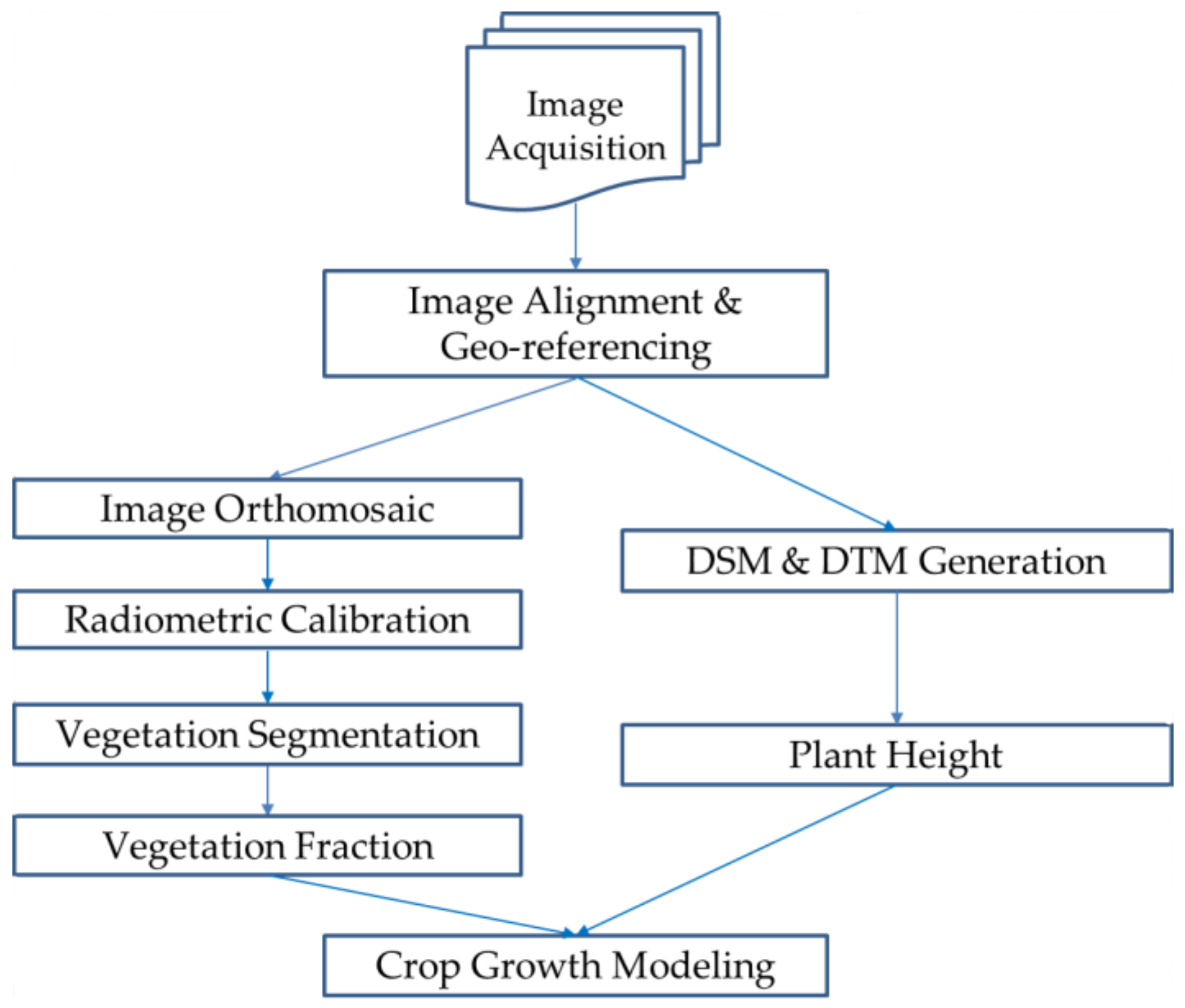
44]. The emergence of structure from motion (SfM)-based software has enabled efficient creation of 3D point clouds and super high detailed ortho-photos without LiDAR sensors [
45,
46]. The SfM photogrammetry is a computer vision method that offers high resolution 3D topographic or structural reconstruction from overlapping imagery [
47]. In principle, SfM performs a bundle adjustment among UAV images based on matching features between the overlapped images to estimate interior and exterior orientation of the onboard sensor. The first step of SfM algorithms is to extract features in each image that can be matched to corresponding features in other images for establishing relative location and parameters of the sensor. The key to SfM methods is the ability to calculate camera position, orientation, and scene geometry purely from the set of overlapping images provided, offering a simple processing workflow compared to alternative photogrammetry techniques [
48,
49]. The workflow of SfM for generating 3D digital reconstructions of landscapes or scenes makes it applicable in a variety of research fields including the modeling of urban and vegetation features. However, the SfM approach with vegetation has proven more difficult than with urban and other features because of the more complex and inconsistent structures resulting from leaf gaps, repeating structures of the same color, and random geometrics. Nevertheless, satisfactory results of vegetation modeling that estimates canopy height with SfM have been reported using colored field markers and increasing the number of acquired photographs.
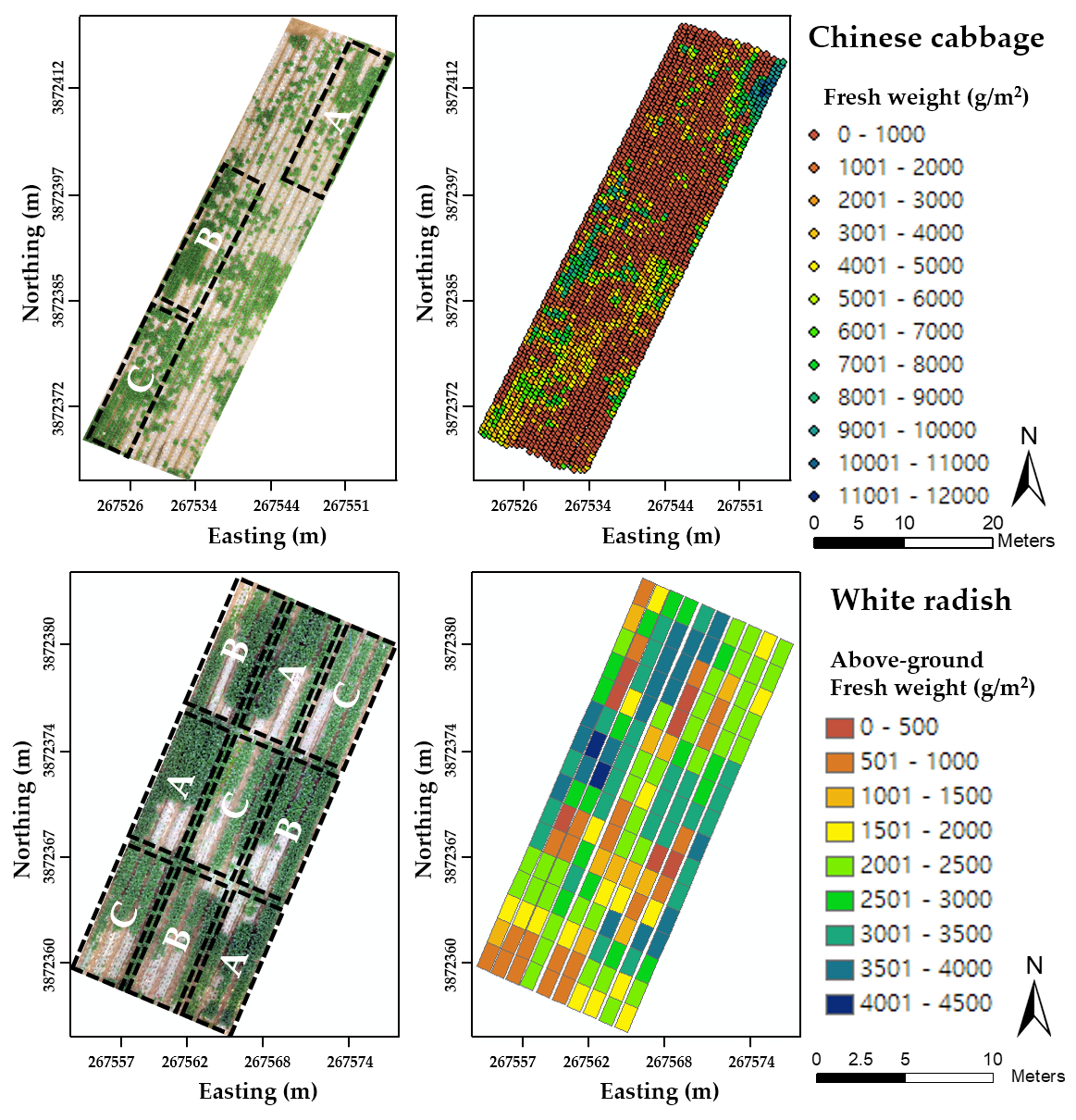
Chinese cabbage (
Brassica rapa subsp.
pekinensis) and white radish (
Raphanus sativus) are commonly cultivated in Korea because they are the main ingredients in Kimchi [
50,
51]. On-site monitoring of their growth status in the field using UAVs with SfM can allow the identification of spatial variation in various biophysical factors, such as canopy coverage, leaf area, and plant height, thereby helping to efficiently regulate the application of fertilizers and water as well as accurately estimate yields prior to harvest. Although previous studies have evaluated the effectiveness of the UAV system for agricultural purposes, yield estimation of Chinese cabbage and white radish using a UAV with only an RGB camera has not yet been studied.
The overall goal of this study was to develop UAV-RGB imagery-based crop growth estimation models that can quantify various biophysical parameters of Chinese cabbage and white radish over the entire growing season, as a means of assessing growth status and estimating potential yields before harvest. Specific objectives were (i) to develop regression models consisting of RGB-based vegetation index and SfM-estimated plant height that can quantify four different biophysical parameters of Chinese cabbage and white radish crops, i.e., leaf length, leaf count, leaf area, and fresh weight, and (ii) to investigate applicability of the developed regression models to a separate dataset of UAV-RGB images obtained from a different year for quantitative analysis of growth status of Chinese cabbage and white radish during the growing season.
4. Discussion
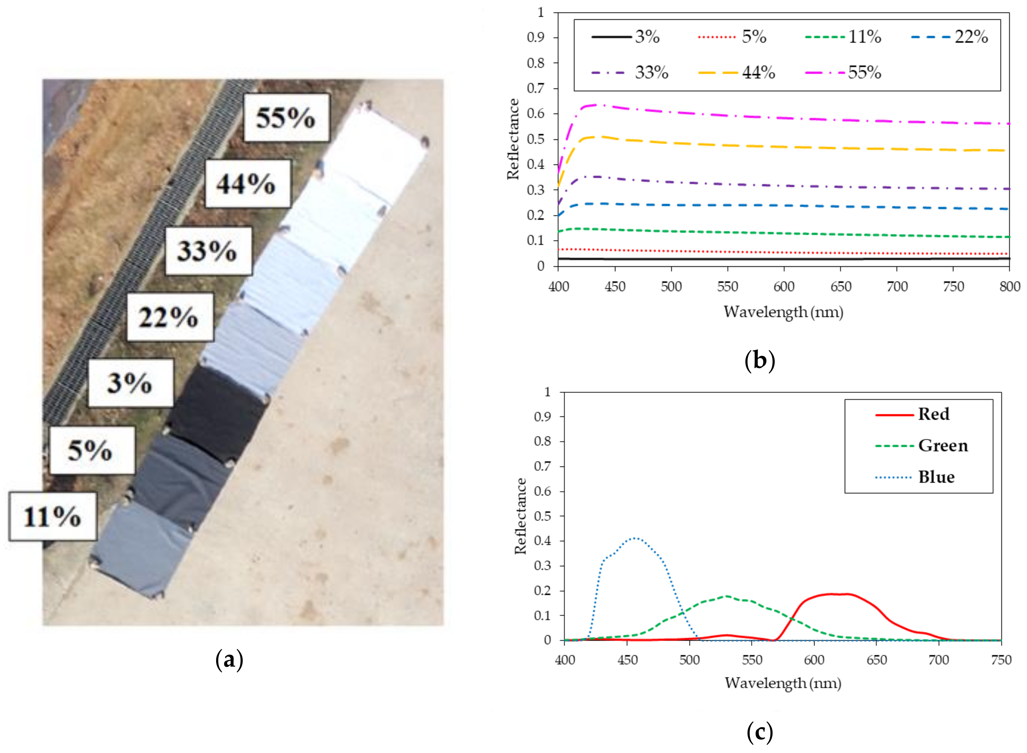
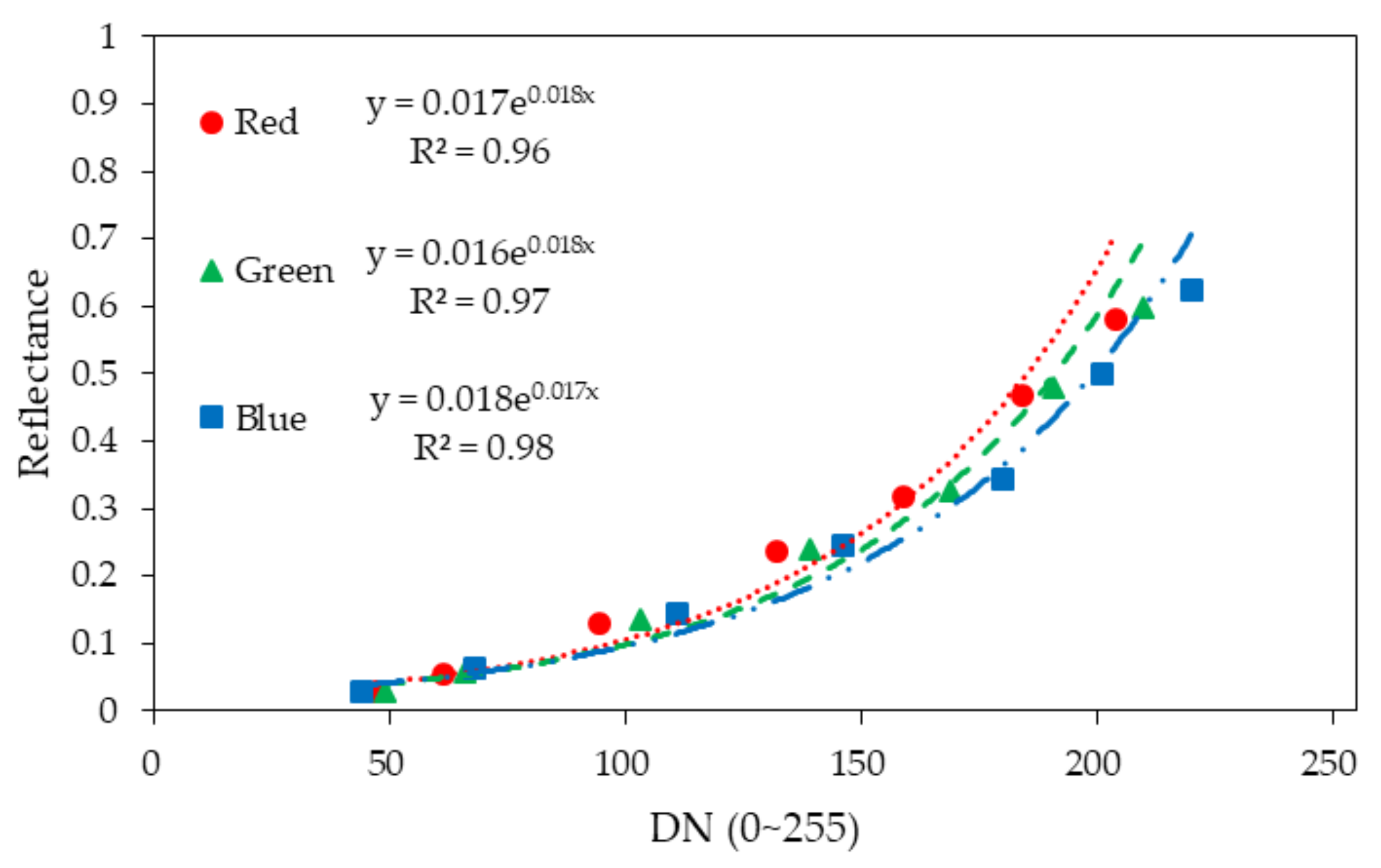
In analyzing multi-temporal UAV images, radiometric calibration is required to minimize the effects of ever-changing light and atmospheric conditions on UAV images taken at different times. Yun et al. conducted radiometric calibration based on the empirical line method [
56] using color-scale calibration targets [
23]. The results showed linear relationships between DNs and reflectance spectra with R
2 ranging from 0.85 to 0.99. However, in general, since the linear relationship might not be suitable when high saturation effects at high DN values are observed. In this study, it was found that the RGB band DNs were exponentially proportional to reflectance values obtained with gray-scale calibration targets, showing significant relationships with R
2 ranging from 0.93 to 0.99 (
Table 4). Therefore, their reflectance data could be normalized to minimize the effect of varying sunlight conditions on UAV-RGB images.
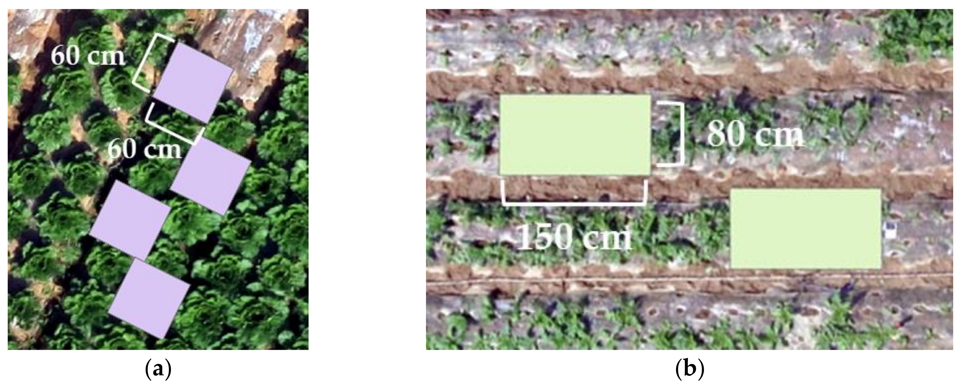
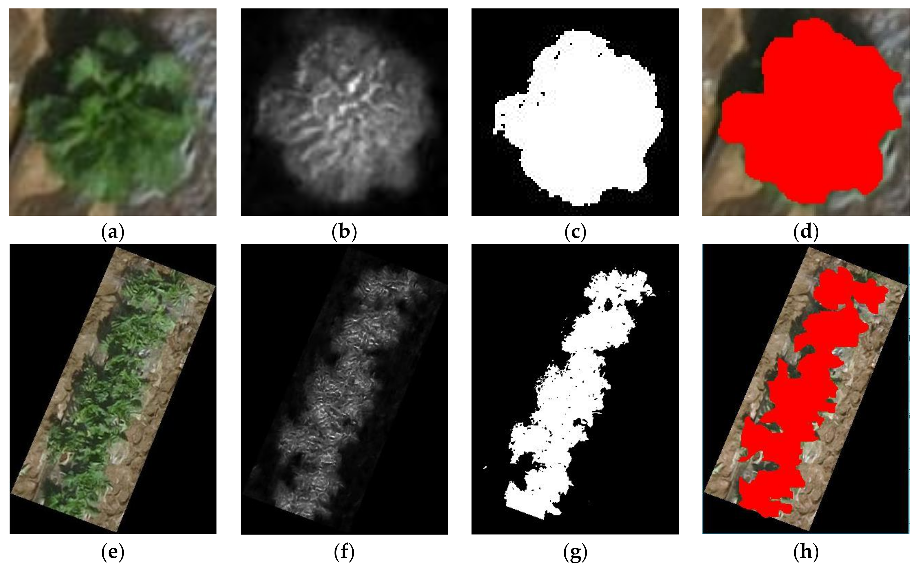
Excess green (ExG) is an efficient vegetation index that can separate crops from a background that includes a mixture of soil and other interfering objects in images with only RGB band. In a study by Torres-Sánchez et al., ExG was used for multi-temporal mapping of the vegetation fraction from UAV images [
15]. In our study, the ExG was applied to automatic crop segmentation with Otsu threshold (
Figure 8). The segmentation results obtained using 10 samples taken from each of randomly selected Chinese cabbage and white radish showed errors ranging from −8.72% to 6.01% for Chinese cabbage and from −14.9% to 17.1% for white radish (
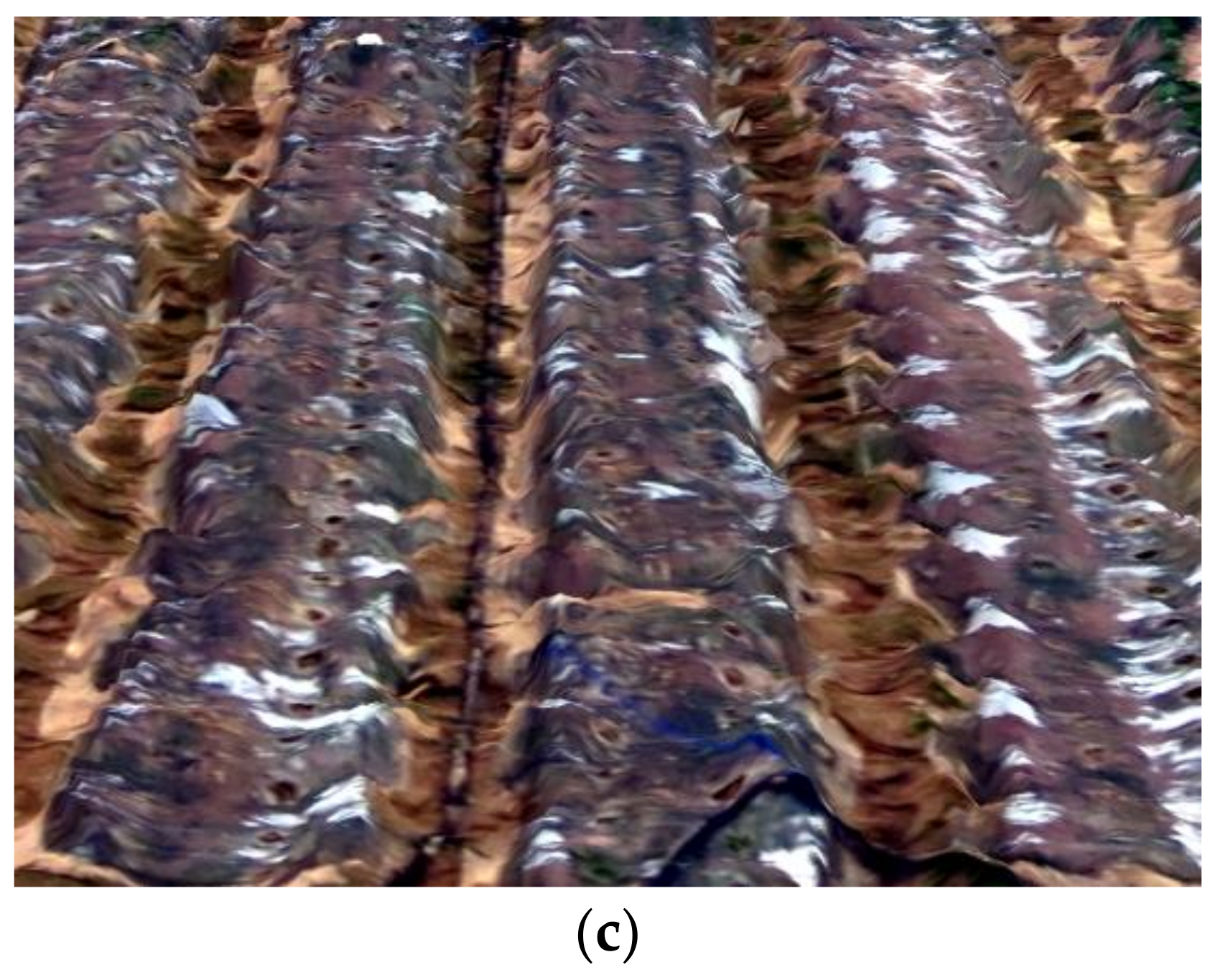
Table 5). This indicates that use of the Otsu threshold method based on the ExG would be satisfactory in segmenting crop images from a background consisting of soil and plastic mulch with accuracies >80%. As mentioned earlier, relatively higher errors were found in the early growth stage of white radish because the boundary area between white radish and background was blurred because of the growth characteristics of white radish, which had overlapping leaves (
Figure 8g). This requires the use of a robust image processing method to improve the segmentation performance for up to 30-day-old white radishes with overlapping leaves.
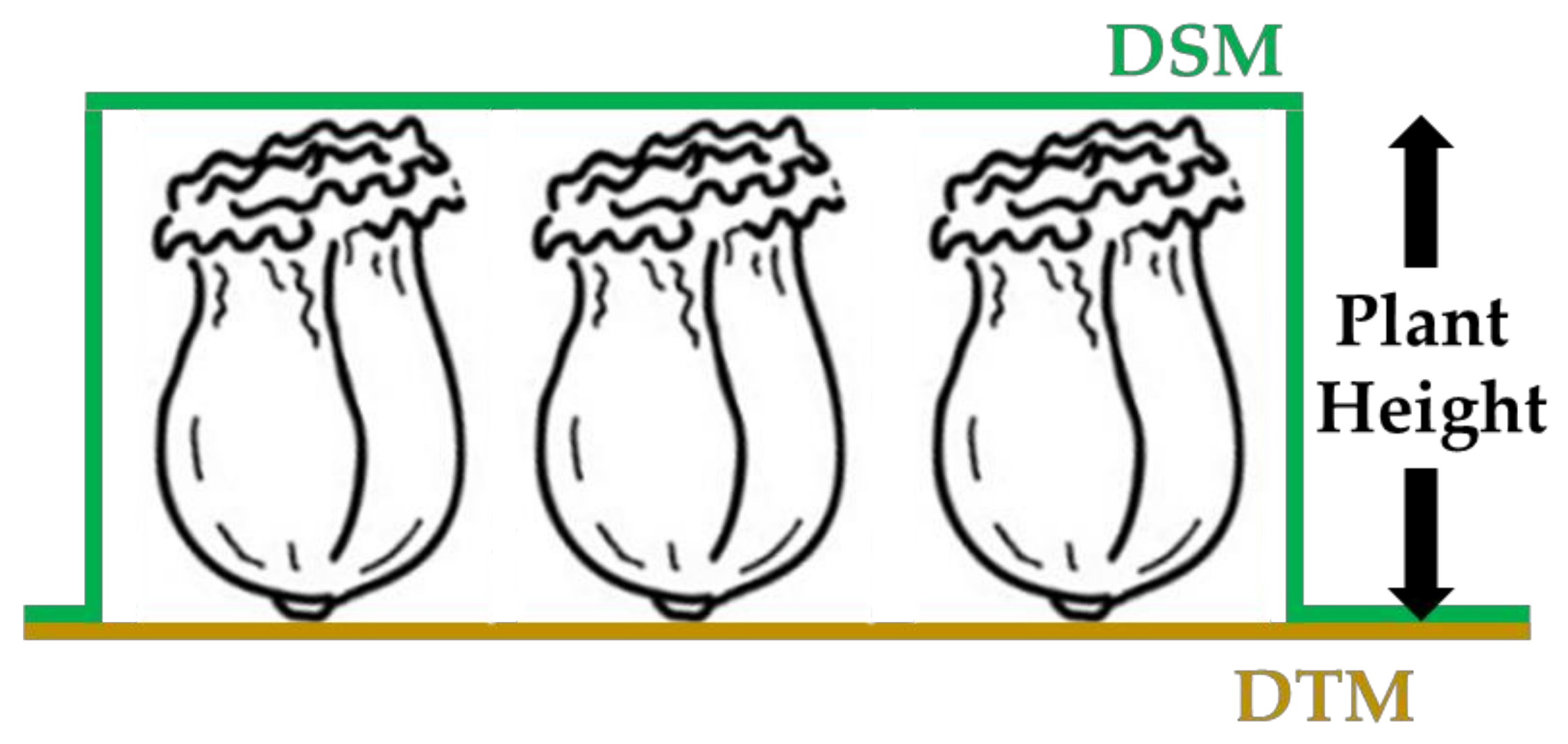
Plant height can be obtained using CSMs [
39,
40]. In the previous studies, the CSMs have been applied to various crops such as sugar, beets, rice, and summer barely [
24,
39,
40,
41]. At the same time, the emergence of SfM-based software has enabled efficient creation of 3D point clouds and super high detailed ortho-photos [
45,
46]. In this study, the SfM algorithm estimated plant heights of Chinese cabbage and white radish, with approximately 1:1 relationships and coefficients of determination (R
2) >0.9 between the heights determined by both the SfM method and manually using a 1 m ruler (
Figure 10). However, the height estimates retained offsets of −6.59 and −1.86 cm for Chinese cabbage and white radish crops between estimated and actual heights. As mentioned in previous studies by Bendig et al. [
24,
39] and Ruiz et al. [
62], this might be related to an inherent error in vertical locations measured with the RTK-GPS that affects the accuracy of GCPs used to correct georeferenced data on UAV images. Another reason responsible for the height measurement error might be the use of a ruler to measure the maximum heights of the crops. Nevertheless, the overall results showed an improvement in accuracy compared to similar studies [
24,
39,
61,
63].
Several studies have applied UAV images to modeling crop growth over the growing season. Bendig et al. applied crop surface models and various vegetation indices to estimate biomass of barely [
64]. Brocks and Bareth also conducted biomass estimation of barley using plant height with crop surface models showing R
2 between 0.55 and 0.79 for dry biomass [
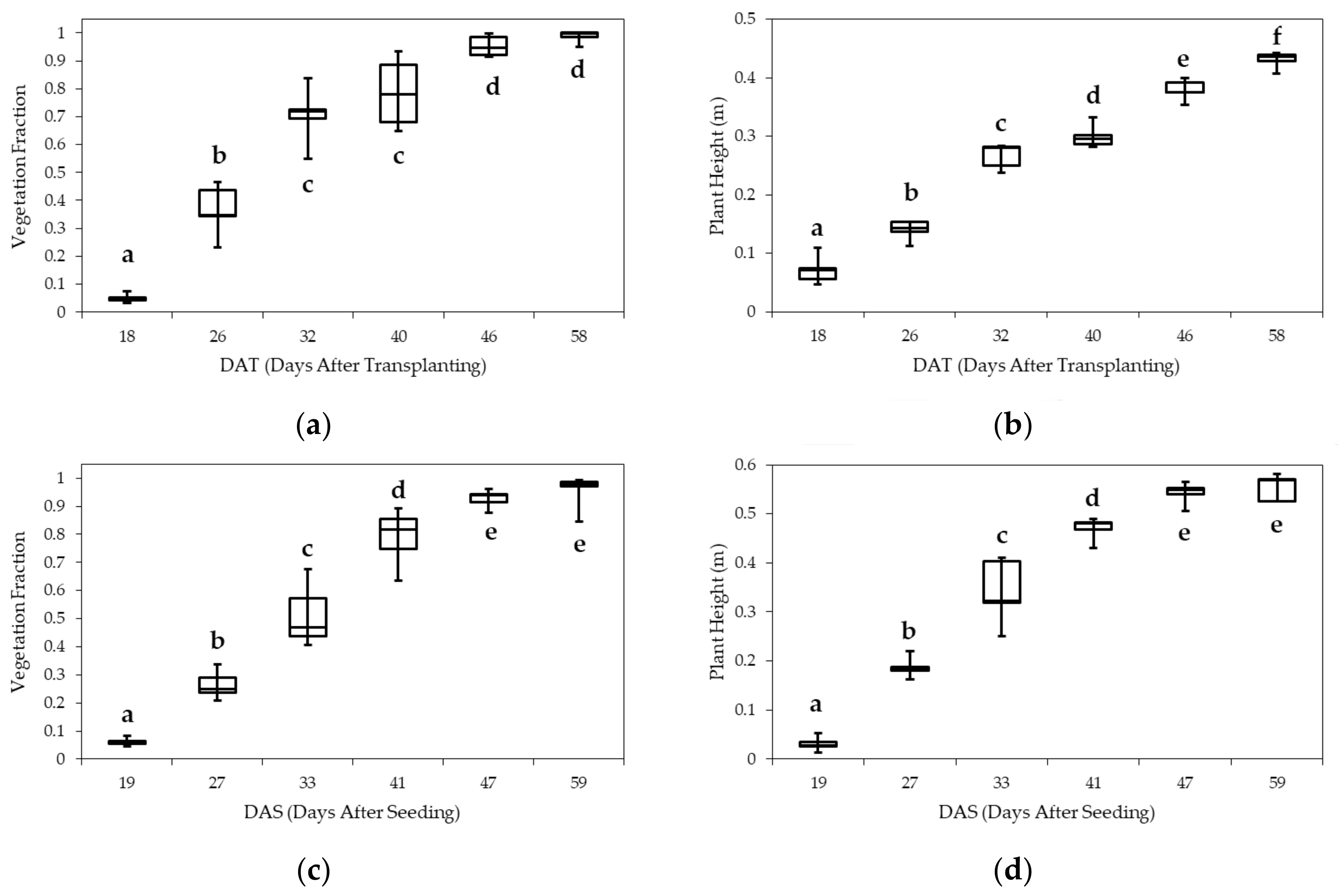
65]. Although many studies have been conducted, yield estimation of Chinese cabbage and white radish using a UAV with an RGB camera has not yet been studied. In this study, prior to building growth estimation models for Chinese cabbage and white radish based on UAV images, time-series analysis of the VF and PH was conducted to characterize their changes with respect to time (
Figure 11). As expected from the results of some previous studies [
15,
23,
61], both VF and PH were linearly proportional to DAT and DAS due to an increase in canopy greenness over time. Saturation phenomena for both the VF and PH were observed, however, beginning from 46 DAT for Chinese cabbage and 47 DAS for white radish, which are similar to the general growth patterns of crops [
66]. Therefore, the saturated VF and PH data were not used to build multiple linear regression models in this study. As shown in
Table 5, it was found that on average, relatively high correlation coefficients existed between the biophysical parameters and the VF compared to the PH data. A possible cause might be explained by the growth characteristics of Chinese cabbage and white radish with a narrower PH range of lower than 60 cm as compared to those obtained with other crops, such as maize and sorghum growing higher than 1 m, whereas Chinese cabbage and white radish grow relatively fast, producing a higher change in VF in almost 2 months.
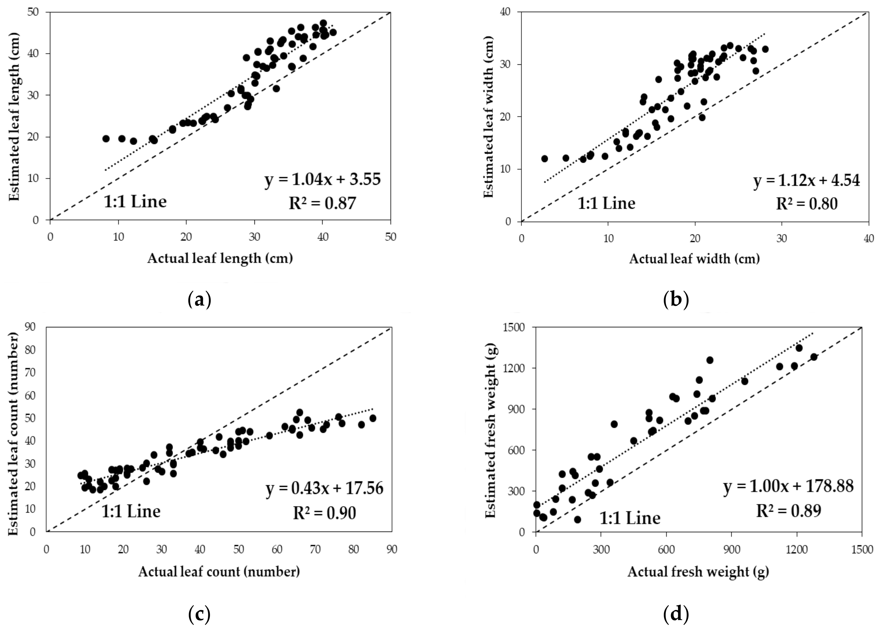
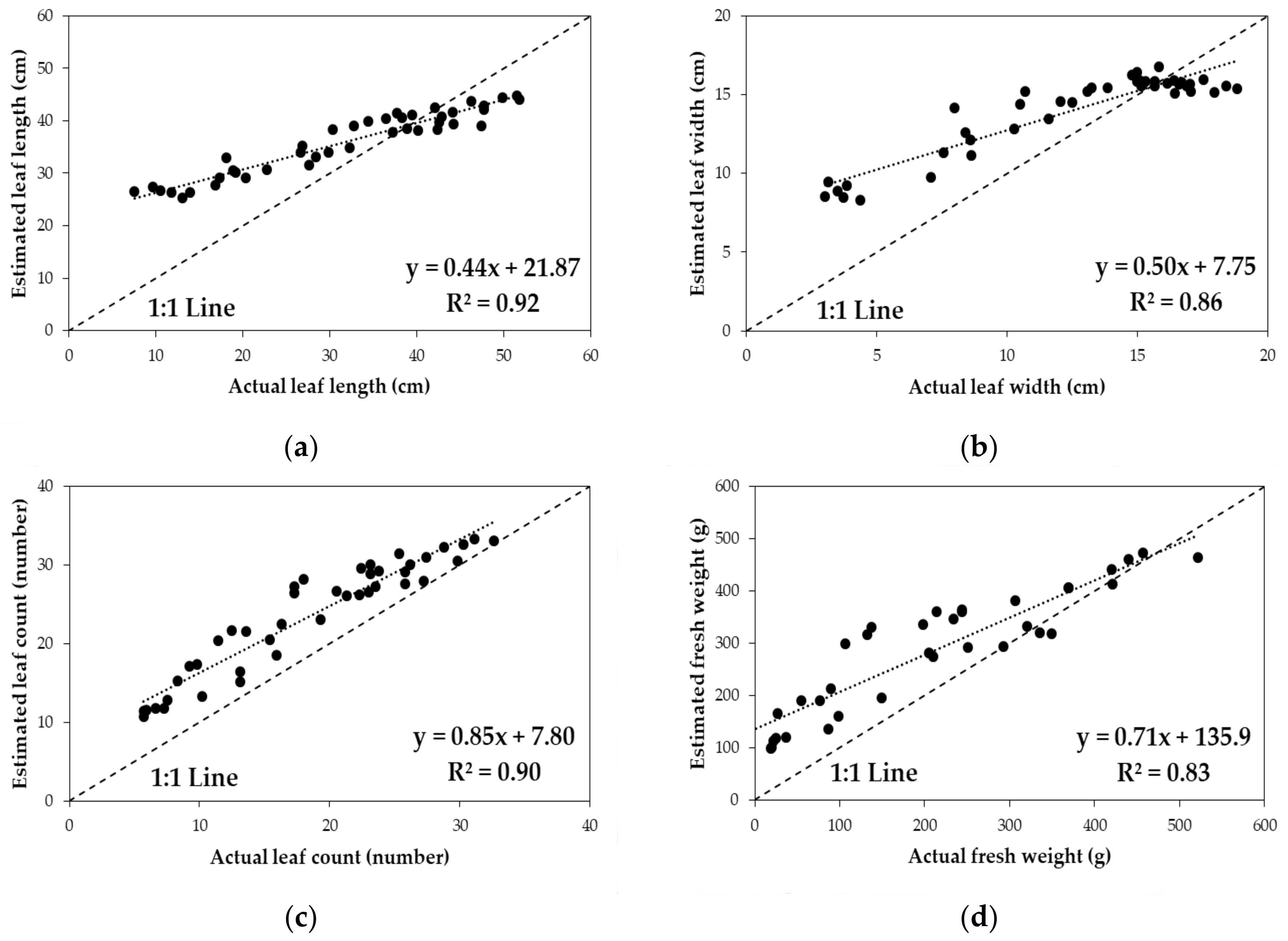
Multiple regression equations for Chinese cabbage and white radish developed from this study, using three predictor variables (VF, PH, and VF × PH) and four different response variables (fresh weight, leaf length, leaf width, and leaf count), provided good fits (R
2 > 0.8) except for relatively decreased estimations in leaf width and count for white radish (R
2 = 0.68 and 0.76, respectively). The results of validation testing showed that strong linear relationships (R
2 > 0.76) existing between the developed models and standard methods would make it possible to use UAV-RGB images for predicting biophysical properties of the two crops in a quantitative manner. However, on average, the prediction accuracies for white radish were worse than those for Chinese cabbage. Likely causes for the lower estimates of white radish growth status might be related to the higher irregularity and narrower leaves of white radish, thereby reducing the performance of the image segmentation due to a difficulty in extracting white radish from the background (
Table 5). An improvement in image segmentation would enhance the ability of the UAV system to estimate the biophysical parameters of white radish.
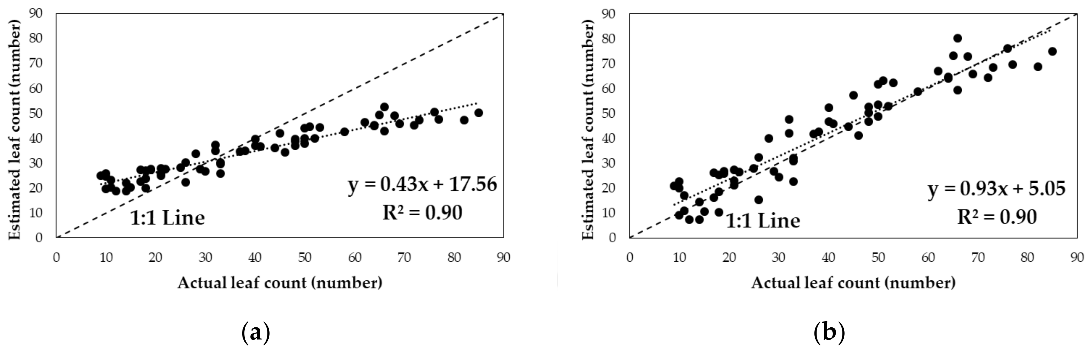
In addition, there was an issue to address slopes of non-unity and offsets of non-zero in the validation testing. For example, leaf count of Chinese cabbage and other biophysical parameters of white radish were highly underestimated when using the UAV image-based estimation model (
Figure 14 and
Figure 15). Possible causes responsible for the lower estimates of leaf count with the UAV system are difficult to explain. However, it might be related to limited spatial resolutions of the RGB images obtained with the UAV flying at 20 m that could not separate their individual leaves with an acceptable level of accuracy. The slopes and offsets can be adjusted using a two-point normalization method. The two-point normalization method is an algorithm to compensate for differences in slope and offset between model estimates and actual values prior to analysis using two known samples of different values [
67]. When using the two-point normalization, it is necessary to select two known samples having the highest difference in growth status if possible to maximize the effect of the two-point normalization using a wide range of data. The slope is directly compensated by comparing the actual value obtained based on destructive sampling and the predicted value obtained with the UAV-RGB system. As shown in
Figure 16, it is apparent that the estimated leaf count can be adjusted, improving the slope and offset from 0.43 to 0.93 and from 17.56 to 5.05, respectively, after two-point normalization. In addition, when the accuracy was assessed using a RMSE [
68], the RMSE of leaf count was decreased from 13.31 to 7.23 by use of the two-point normalization. Future studies include the application of the developed UAV-estimated models in conjunction with use of the two-point normalization method to commercial fields growing Chinese cabbage and white radish.


 and
and 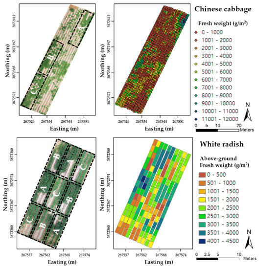


