Article

Unsupervised Classification Algorithm for Early Weed Detection in Row-Crops by Combining Spatial and Spectral Information

1
Agroécologie, AgroSup Dijon, INRA, Université Bourgogne Franche-Comté, 21000 Dijon, France
2
AIRINOV, 174 Quai de Jemmapes, 75010 Paris, France
*
Author to whom correspondence should be addressed.
Submission received: 22 March 2018 / Revised: 9 May 2018 / Accepted: 11 May 2018 / Published: 15 May 2018
(This article belongs to the Section Remote Sensing in Agriculture and Vegetation)

Abstract

:
In agriculture, reducing herbicide use is a challenge to reduce health and environmental risks while maintaining production yield and quality. Site-specific weed management is a promising way to reach this objective but requires efficient weed detection methods. In this paper, an automatic image processing has been developed to discriminate between crop and weed pixels combining spatial and spectral information extracted from four-band multispectral images. Image data was captured at 3 m above ground, with a camera (multiSPEC 4C, AIRINOV, Paris) mounted on a pole kept manually. For each image, the field of view was approximately 4 m × 3 m and the resolution was 6 mm/pix. The row crop arrangement was first used to discriminate between some crop and weed pixels depending on their location inside or outside of crop rows. Then, these pixels were used to automatically build the training dataset concerning the multispectral features of crop and weed pixel classes. For each image, a specific training dataset was used by a supervised classifier (Support Vector Machine) to classify pixels that cannot be correctly discriminated using only the initial spatial approach. Finally, inter-row pixels were classified as weed and in-row pixels were classified as crop or weed depending on their spectral characteristics. The method was assessed on 14 images captured on maize and sugar beet fields. The contribution of the spatial, spectral and combined information was studied with respect to the classification quality. Our results show the better ability of the spatial and spectral combination algorithm to detect weeds between and within crop rows. They demonstrate the improvement of the weed detection rate and the improvement of its robustness. On all images, the mean value of the weed detection rate was 89% for spatial and spectral combination method, 79% for spatial method, and 75% for spectral method. Moreover, our work shows that the plant in-line sowing can be used to design an automatic image processing and classification algorithm to detect weed without requiring any manual data selection and labelling. Since the method required crop row identification, the method is suitable for wide-row crops and high spatial resolution images (at least 6 mm/pix).

Graphical Abstract

1. Introduction

In conventional cropping systems, chemical inputs have been adopted to increase agricultural production. Unfortunately, the use of large amount of chemicals raises serious problems relating to water contamination, health risks (for applicators and food consumers), biodiversity reduction, and risk of development of herbicide-resistance weeds. Thus, the challenge is still reducing herbicide use whilst maintaining production efficiency, avoiding weeds from reducing yields and harvest quality [1].
To achieve this objective, one way consists of site specific weed management [2,3] by triggering a specific chemical or physical (e.g., mechanical, thermal, and electrical) action only where weeds lie. For example, in the case of chemical tools, various works have already demonstrated the technical feasibility of precision weed control implements. Numerous works addressed the use of chemical sprayer able to turn on or off boom sections or individual nozzles [4,5,6,7,8] to applied herbicides specifically on clusters or individual weed plants. Concerning physical weed management, technologies had also been developed to guide weeding devices according to weed detection in fields [9].
Concerning the detection and the localization of weeds in crops various approaches have been developed which can be first distinguished on the basis of the platform (satellite, aerial, or terrestrial vehicle) and the sensor (imaging or non-imaging sensor) used for image acquisition. In the last decade, Unmanned Aerial Vehicles (UAVs) became a very popular platform to carry acquisition systems and thus monitor agricultural fields [10]. Compared to satellite or manned airborne, the main advantages of UAVs are their low cost, low operational complexity, fast results, high spatial and temporal resolution, and therefore their operational ability. In recent years, numerous papers addressed the use of UAVs for weed detection and mapping. An overview of the adoption of UAVs in weed research work can be found in Rasmussen, et al. [11]. Compared to terrestrial vehicles, remote sensing using UAVs is a more effective approach to provide a weed map on large areas. Nevertheless, as specified by Lamb and Brown [12], remote sensing to detect and map weeds requires: (1) sufficient differences in spectral reflectance or texture between weeds and soil or crops and (2) an appropriate spatial and spectral resolution for the acquisition system.
Various authors demonstrated that weeds and crops can be discriminated using their reflectance spectra [13,14,15,16,17,18]. Nevertheless, when data are captured in field by small UAVs, the design of robust and efficient spectral-based detection methods encounters three main difficulties: the loading limit entails the use of a limited number of spectral bands; the spectral information is affected by the uncontrolled field conditions (e.g., sun height, cloud cover, shadow, and dust), and the leaf spectral reflectance changes with physiological stress [19]. Due to these perturbations and information variations, it is difficult to design automatic and generalized algorithms only based on spectral information which is moreover limited to a few number of channels.
At the present time, for weed mapping, sensors used on UAVs are commonly multi-spectral imaging sensors. Several studies have demonstrated that the choice of at least four spectral bands provided better results than the use of standard RGB camera especially when near infra-red (NIR) information was used [20,21]. In particular, the use of NIR information improves the separation between the vegetation and the background (i.e., soil) in image pre-processing [22]. In recent studies, Pérez-Ortiz, et al. [23] used an RGB camera, Peña, et al. [24] used a six-band multispectral camera (i.e., bandpass filters centred at 530, 550, 570, 670, 700, and 800 nm), López-Granados, et al. [25] used an RGB camera and a six-band multispectral camera (i.e., bandpass filters centred at 450, 530, 670, 700, 740, and 780 nm).
Various methods have been proposed to discriminate weeds and crops in UAV multispectral images. In most of these methods, the first step consists in detecting the vegetation in the image by computing a vegetation index and obtaining a vegetation mask by thresholding. The most common vegetation indices to separate the vegetation from the soil are the Normalized Difference Vegetation Index (NDVI) [26] used when NIR information is available and the Excess Green index (ExG or 2g-r-b index defined by Woebbecke, et al. [27]) when RGB images are used. This vegetation detection approach has been used as pre-processing step of weed detection in numerous recent works [24,25,28,29].
Then, geometrical information can be used to distinguish between crop and weeds. Various shape analysis techniques [24,30,31] or textural-based methods were suggested [28,32]. These techniques required images with high spatial resolutions and sufficient shape differences between crop and weeds. In practice, the use of shape or textural-based method is all the more difficult when images are captured at an early stage of plant growth. Another key spatial information to distinguish between crop and weeds is the geometry of plant arrangement. In particular, numerous works developed automatic seed row detection and localization methods. These techniques have been first developed for vehicle or implement guidance [33,34] and have been used for inter-row mechanical weed control assuming that the plants lying in the inter-row area were weeds [35]. Finally, these techniques have also been used to map weeds in fields [36]. Then, the same assumption was made to process aerial and UAV images and detect weeds in the inter-row. Vioix, et al. [37] extracted the spatial information by using a frequency analysis of the image and used a Gabor filter [38] to detect crop rows on the vegetation images. Peña, Torres-Sánchez, de Castro, Kelly and López-Granados [24] used a segmentation approach called Object-Based Image Analysis (OBIA). One advantage of the OBIA approach lied in the generation of spectrally similar regions with a minimum size. Thus, the authors developed a method based on this segmentation to identify crop rows and then discriminate between crop plants and weeds by considering their relative positions. On a field of maize at 4–6 leave stage, the method was used to classify areas in low, moderate or high infestation level. The overall accuracy was 86%. These works mainly exploited spatial information. They provided good results regarding the detection of weeds between crop rows but were not designed to detect weeds located in crop rows. In these works, the use of spectral information was limited to the extraction of a vegetation image using a simple thresholding step on vegetation indices or a more advanced segmentation step exploiting spectral features [24]. Consequently spectral information was not fully exploited in these approaches which were mainly based on crop row detection.
In order to improve weed detection, various authors proposed the use of both spatial and spectral information in the classification step. Vioix [39] proposed to merge spatial and spectral information to improve the discrimination between crops and weeds. Visually good results were obtained using a method based on Bayes probabilities or considering pixel neighborhood relationships. For invasive weed species in natural environment, Hung, et al. [40] developed a feature learning based approach using color information (on RGB images), edge information, and texture information. The work of Peña, Torres-Sánchez, de Castro, Kelly and López-Granados [24] had been extended to make greater use of spectral information but also shape information, spatial information and textural information. Thus, López-Granados, Torres-Sánchez, Serrano-Pérez, de Castro, Mesas-Carrascosa and Peña [25] used the same OBIA method. For linear vegetation objects that are in contact with crop rows and that are difficult to classify regarding only spatial information, the authors classified them following a criterion of minimum spectral distance. Thus, an unclassified vegetation object was assigned to the crop or the weed class depending on the degree of spectral similarity of their NDVI or ExG values. Pérez-Ortiz, et al. [41] combined the use of data derived from the OBIA method with the use of a supervised classifier (Support Vector Machine classifier). They demonstrated the object-based analysis reached better results than a pixel-based approach limited to spectral information. For each object, the OBIA method provided spectral information (histograms or statistical metrics), a vegetation index (ExG) and shape information, which could be used by the classifier. In sunflower fields (4–6 leave stage) the classification accuracy reached 96%. For the classifier, the training procedure consisted in manually labelling 90 objects per class (soil, weeds, and crop). Combining various kind of information, an important benefit of the method was that it was adapted to the detection of weed not only between but also within the crop row. Pérez-Ortiz, Peña, Gutiérrez, Torres-Sánchez, Hervás-Martínez and López-Granados [23] completed the previous work by developing an automatic method to select the most representative patterns to construct a reliable training set for the classifier. They also developed an automatic feature selection process to select the more useful object features for weed mapping. The study was tested on sunflower and maize crops. These refinements improved the method and helped the user in the labelling task. A first automatic labelling step was performed to build the training data; nevertheless a manual verification of the labelled patterns is still required for these data. Lottes, Khanna, Pfeifer, Siegwart and Stachniss [22] used an object-based and a keypoint-based approach. They proposed a classification system taking into account several spectral and geometrical features. The geometrical features were based on a line extraction using the Hough Transform when crop row existed but also on spatial relationships between objects (without exploiting the line feature). Their classification system is adapted to RGB-only as well as RGB combined with NIR imagery captured by a UAV. Moreover their method is able to exploit the spatial plant arrangement with prior information regarding crop row arrangement or without explicitly specifying the geometrical arrangement. The method used a multi-class Random Forest classification and required a training dataset. The overall accuracy of the classification between crop and weeds was 96% in sugar beet fields. Recently, Gao, et al. [42] suggested combing the detection of inter-row weed using a Hough transform based algorithm with an OBIA procedure and a Random Forest classifier. With this approach, they proposed a semi-automatic procedure in which inter-row vegetation objects were automatically labeled as training data for weeds. De Castro, et al. [43] developed an OBIA algorithm using a Random Forest classifier and taking advantage of plant height information derived from Digital Surface Models. Surface Model. In the row, the vegetation object height was used to pre-classify as crops the plants higher than the average height in the crop row. Outside the crop rows, all plants were classified as weeds. Using this technique, the authors proposed an automatic algorithm to detect weeds between and within crop rows without any manual training. The 3D reconstruction of crops required the capture of images with a large overlap. The authors underlined the ability of the method to detect weeds was significantly affected by image spatial resolution. The method was assessed on sunflower and cotton fields. The authors indicated that the coefficient of determination computed between the estimated weed coverage and the ground truth was higher than 0.66 in most cases.
The literature demonstrates that the use of supervised classifiers well discriminate weeds from crops when a combination of spatial and spectral information is used as input data. Unfortunately, since supervised classifiers require training data sets, the design of automatic image processing without manual setting or manual data labelling is still challenging.
The objective of this paper is to develop an automatic image processing to detect weeds in row crops without requiring the manual selection of any training data before classification. The approach combines spectral and geometrical information. It assumes that: (1) plants lying in the inter-rows are weeds and (2) weeds lying in the rows are spectrally similar to those located in the inter-rows. This approach is adapted to the detection of weeds between and within crop rows. In this paper, the method was applied on images captured with a four-band multispectral sensor mounted on 3-m pole.
This paper has two main contributions:
(1)
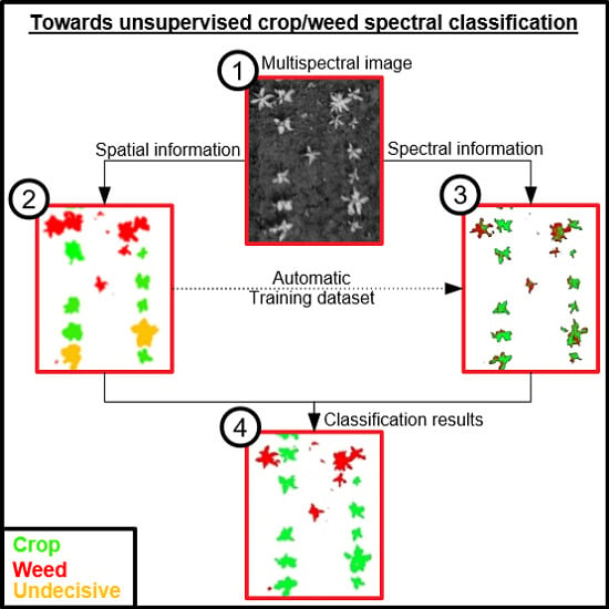
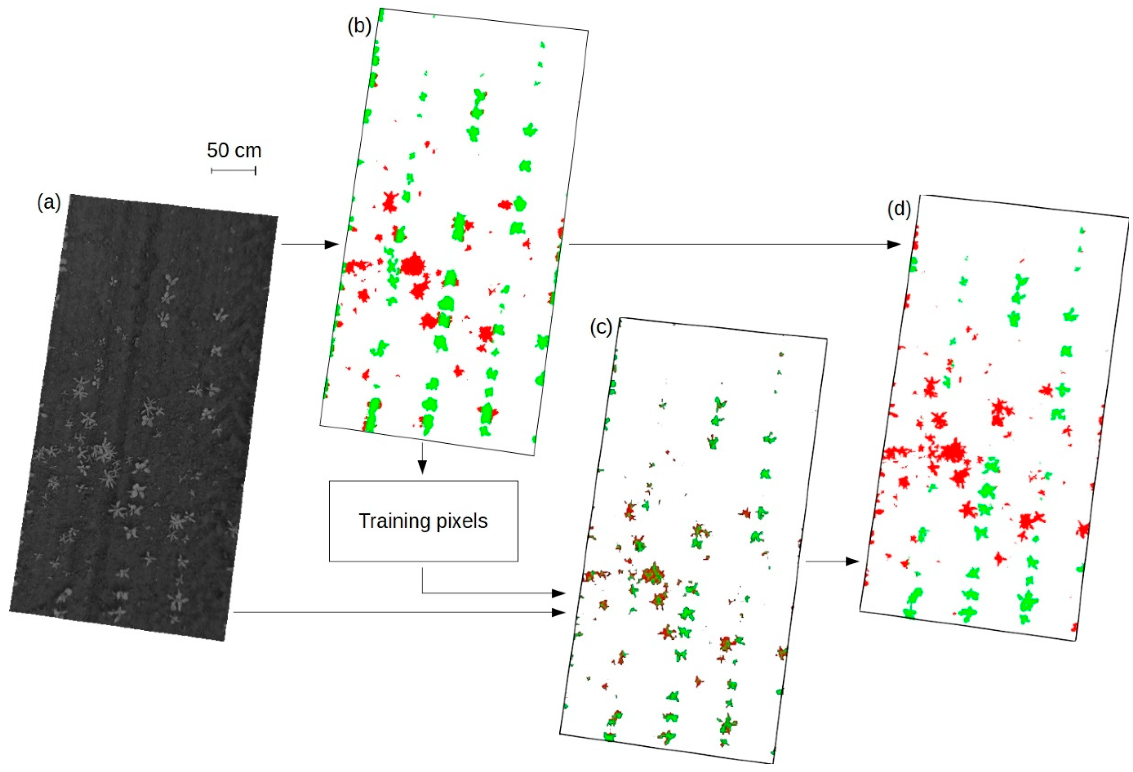
A classification method is developed by combining spectral and spatial information, and by using spatial information to build automatically the training dataset used by a supervised classifier without requiring any manual selection of soil, crop, or weed pixels;
(2)
The contribution of the spatial information alone, the spectral information alone and the combination of spectral and spatial information is analyzed with respect to the classification quality for a set of images captured in sugar beet and maize fields.

2. Materials and Methods

This section first describes the experimental sites, the devices and the data collected in the sites (Section 2.1). Then, the analysis of the data and the images are presented to distinguish between crops and weeds (Section 2.2).

2.1. Site Description and Data Collection

2.1.1. Experimental Sites

Experiments were undertaken in France in April 2015 [44] on commercial fields of maize (15.86 ha, WGS 84: 49.2133°N, 2.6085°E) and sugar beet (7.69 ha, WGS 84: 49.2375°N, 2.76575°E). The acquisition dates were chosen at early crop stages (2–3 leaves), corresponding to the period of post-emergence herbicide applications. At this stage, the crop rows can be clearly identified in the field. The maize (BBCH stage 13, Meier [45]) and sugar beet (BBCH stage 15) commercial fields were located in Oise (north of Paris). The maize field was infested with two dicotyledons, lamb’s quarters (Chenopodium album L.) and thistle (Cirsium arvense L.) from seedling to rosette stage. The sugar beet field was infested by thistle (Cirsium arvense L.) from seedling to rosette stage, wild buckwheat (Fallopia convolvulus) at 4-leaf stage, and rye-grass (Lolium multiflorum) at tillering stage.

2.1.2. Field Data Acquisition

Multispectral images were acquired with a camera mounted on a pole at 3 m above ground. The acquisition system was developed by AIRINOV (Figure 1). It was composed of different sensors including a light sensor and a multispectral imaging system (multiSPEC 4C, AIRINOV, Paris, France). These acquisitions were performed to provide data at a spatial resolution of 6 mm/pixel.
The field of view of the camera produced a 4 m by 3 m image. In each crop field, three squares (5 m × 5 m) regions were used as ground truth. This ground truth consisted in manually locating and identifying each weed. That information was used to label the weed pixels in the image.

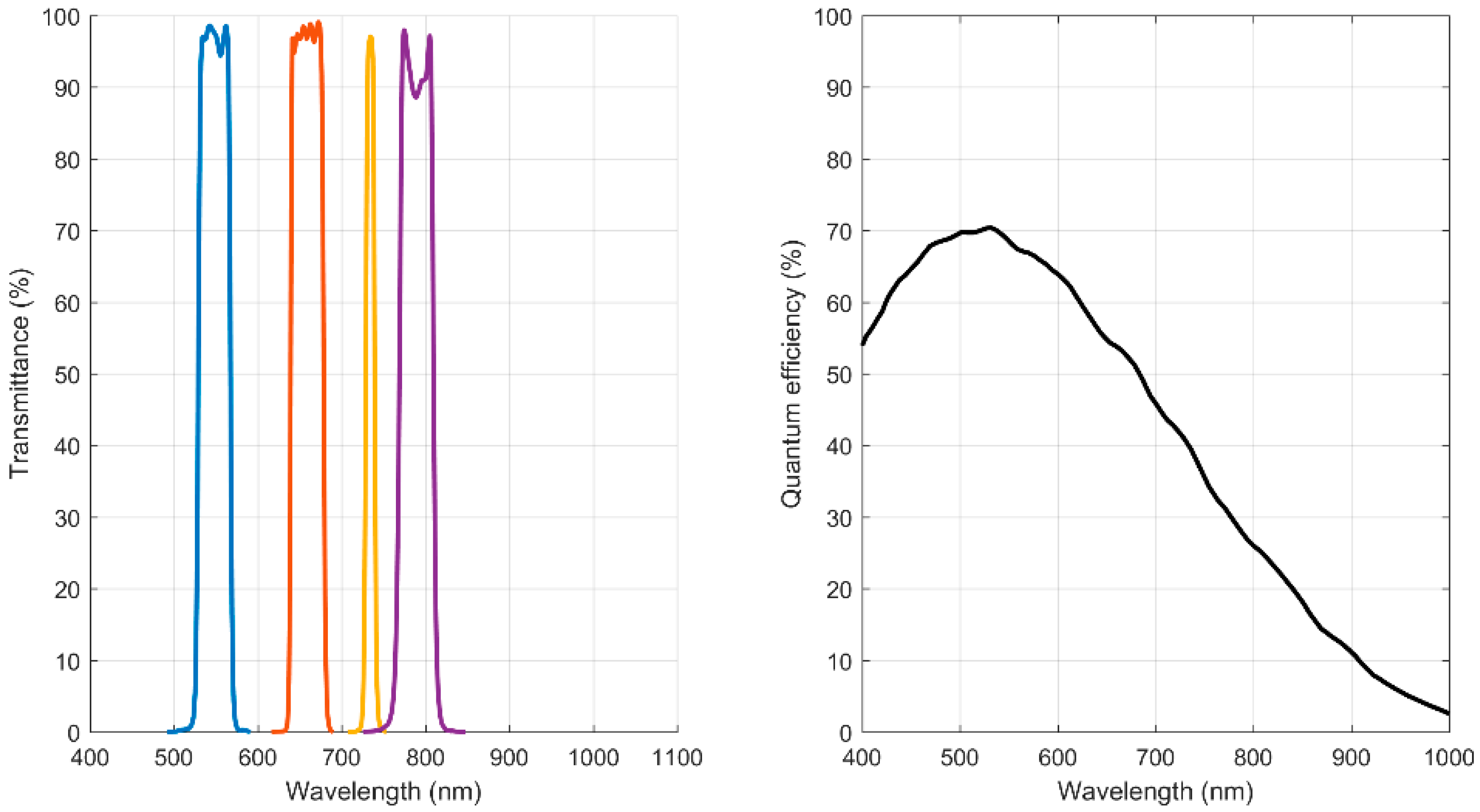
2.1.3. Multispectral Imagery Acquisition

The multispectral imaging system was composed of a light sensor collecting incident light and four CMOS sensors [46]. Each sensor was characterized by a 4.8 mm × 3.6 mm matrix (12 megapixels) and a focal length of 3.8 mm. The camera was used to acquire images in four narrow spectral bands selected using interferential filters centered on 550 nm (green), 660 nm (red), 735 nm (red-edge) and 790 nm (near-infrared) (Figure 2). The spectral resolution (full width at half maximum, FWHM) was 40 nm for the green, red and NIR bands and 10 nm for the red-edge band. The frames (the synchronous acquisition of the 4 bands) were recorded on a SD card. A GPS antenna allowed real time geotagging of the frames. For each of the two fields (maize and sugar beet), data collection was performed over a sunny day around noon. From this dataset, 7 multispectral images with corresponding ground truth were chosen to assess the methods developed in this paper. The images were taken at a frequency of 0.5 Hz (along 5 parallel tracks every 1.5 m), allowing about 80% overlap between them along-track and 66% across-track.

2.2. Data Processing and Analysis

For each field, light conditions have been acquired by the light sensor and the camera on a calibrated reference (neutral gray). The light sensor measured the sunlight variations during the acquisition to automatically correct the differences in illumination between shots. The combination of these measurements allowed to obtain reflectance calibrated multispectral images. These images were radiometrically (vignetting effects) and geometrically corrected (distorsions). Subsequently a photogrammetric software (Pix4DMapper by Pix4D, Switzerland) was used to merge the geotagged frame, process the registration of the four channels and create an orthoimage (covering 5 m × 5 m). This was the overall orthoimage creation process. In this work, the weed detection was performed on individual images before the merging process. These images were chosen to avoid the loss of quality due to the merging process.
Three methods were developed to discriminate crop from weeds and are presented in the following sections. The first one is based on spatial information only, the second one requires manual intervention (to populate the training dataset) to discriminate crop from weeds using only spectral information, the third combine spatial and spectral information to improve classification results and overcome the limits of the previous methods.

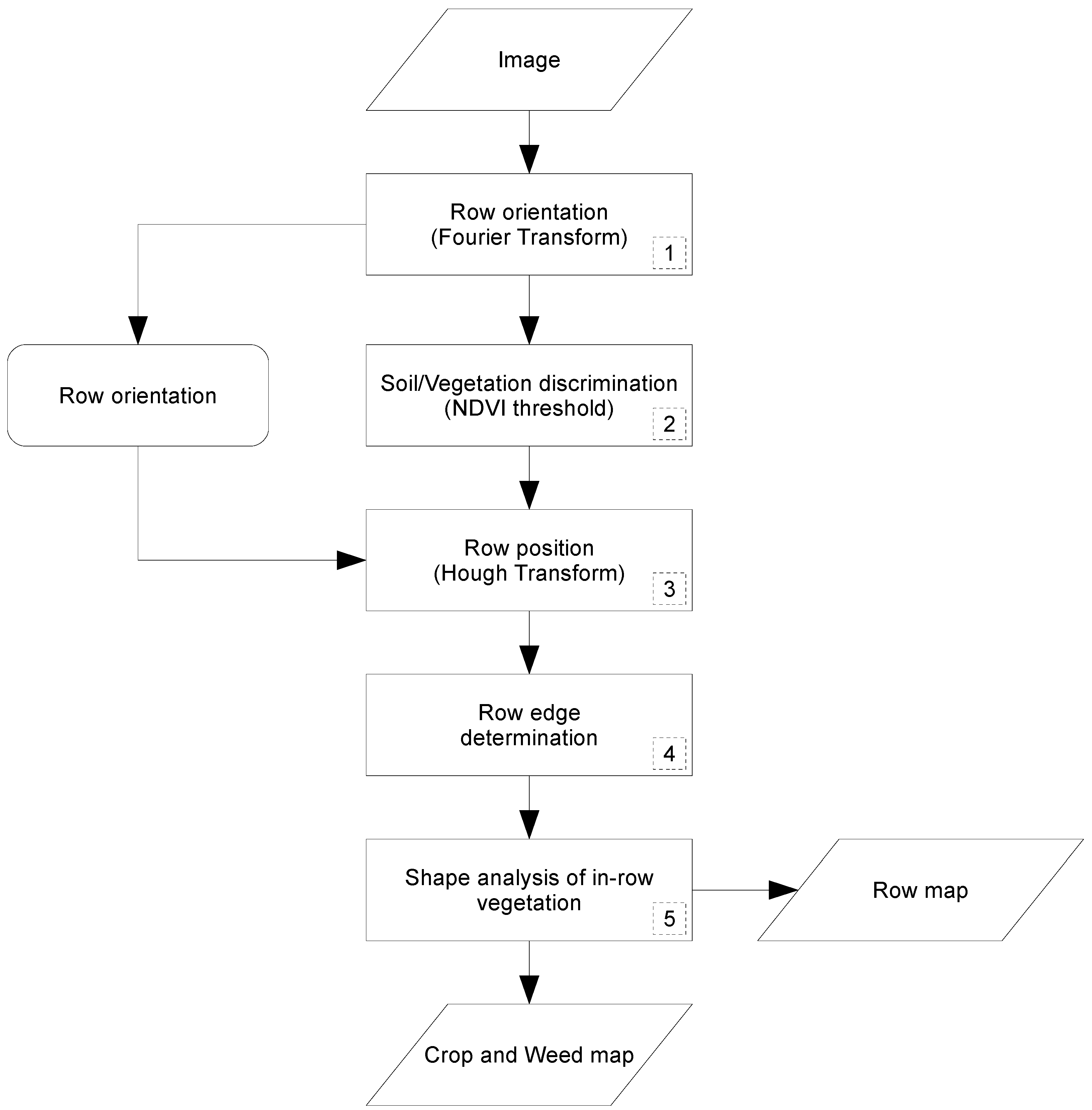
2.2.1. Algorithm Based on Spatial Information

As crops are usually sowed in rows a method was developed to detect these rows and discriminate crop from weeds using this information. This method is composed of multiple steps described in the Figure 3.
The first step is to extract the row orientation using a Fourier Transform [47]. This transform performs a frequency analysis of the image to emphasize row orientation in Fourier Space. Most common orientations are represented by the main peaks which can be isolated with a Gaussian filter. The window size and standard deviation of the Gaussian filter are deduced from the inter-row width (a priori knowledge).
The second step is the discrimination between soil and vegetation pixels using NDVI [48,49] and an automatic threshold based on Otsu [50]. The result is a binary image presenting two classes: Soil and Vegetation.
The third step is the detection of rows using a Hough Transform [51] adapted to detect lines using a polar representation [52]. This representation describes a line with the parameters ( ρ , θ ) where ρ is the distance between the origin and the closest point on the line and θ is the angle between the x axis and the line connecting the origin to that closest point. This step is applied only on vegetation pixels (from step two) and the studied angles are limited to the orientation found in the first step (±2°).
ρ = x × c o s ( θ ) + y × s i n ( θ )
Once the lines representing the rows are found the fourth step is to determine the edges of each row. Each connected component intersected by the detected line is analyzed to find the farthest vegetation pixel (orthogonally to the line) on each side of the line. A linear regression is performed on pixels from the same side to obtain the edge line. Rows are considered to be inside two edge lines, inter-rows are considered outside.
The fifth step is to improve crop/weed discrimination using the shape of connected components. When a connected component is, at least in part, inside the detected edges of a row it can be considered as crop or weed based on its area, orientation and axis length. Figure 4 shows the decision tree used to discriminate crop from weeds.

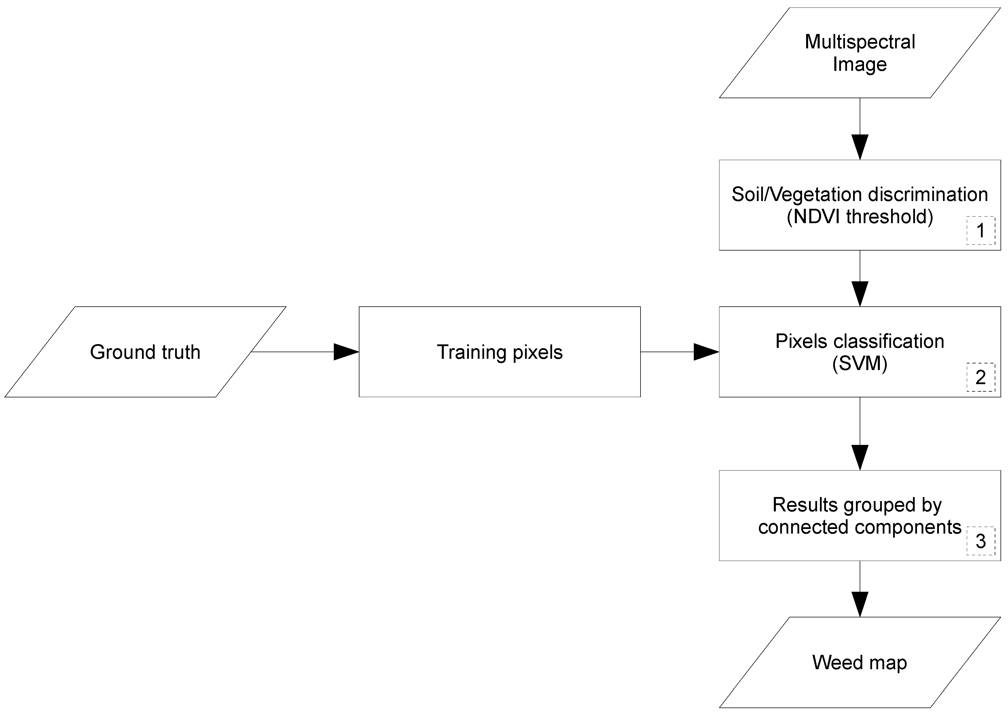
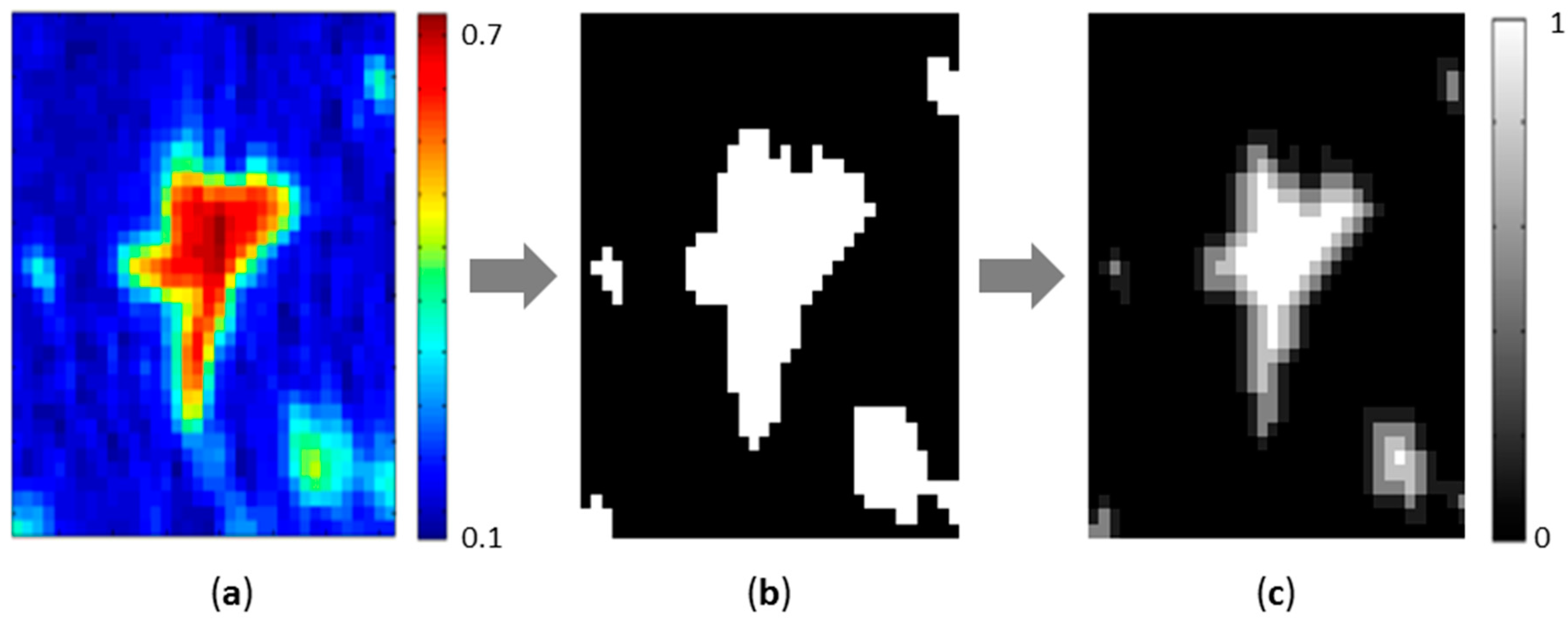
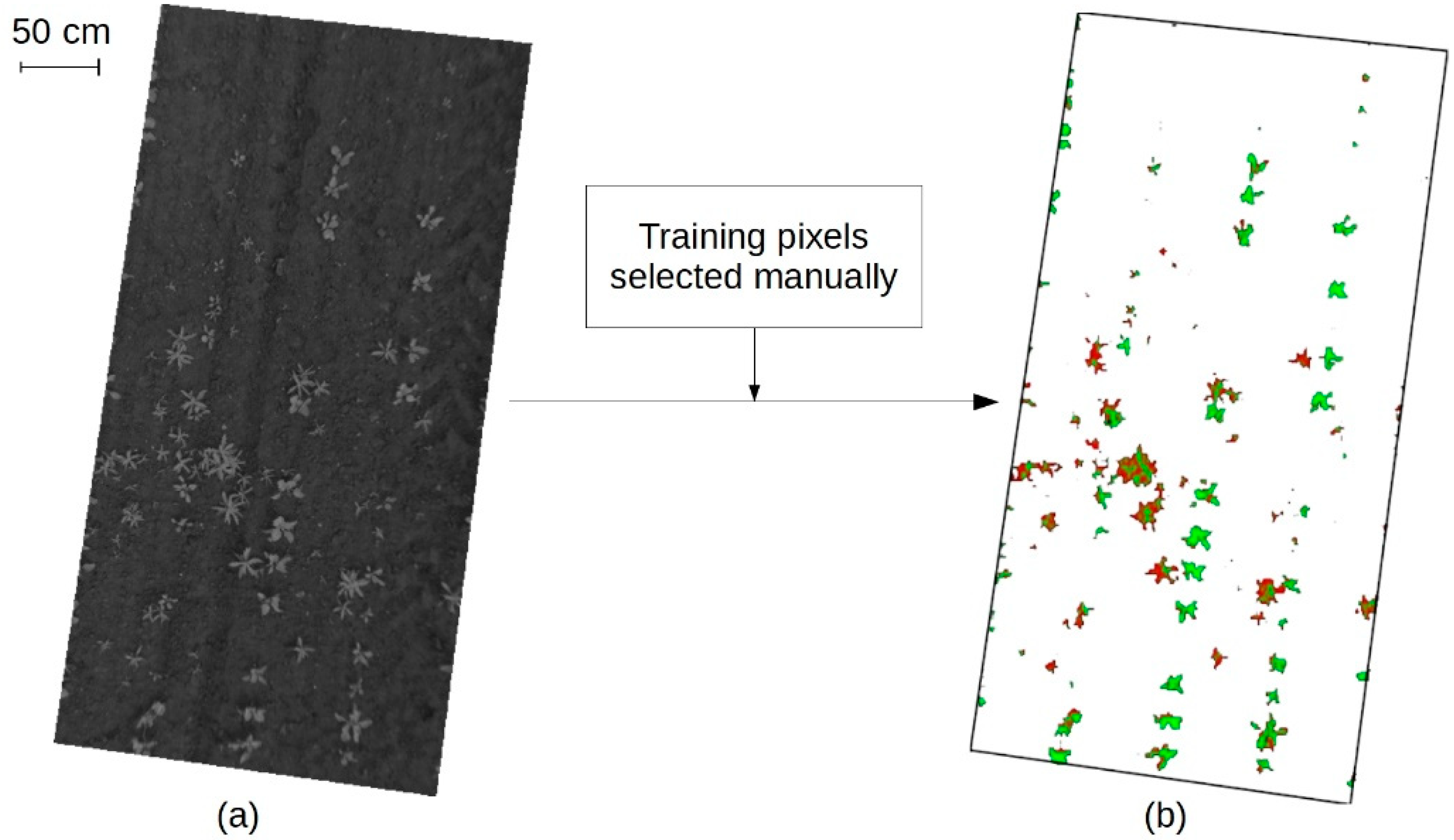
2.2.2. Algorithm Based on Spectral Information

There are two types of methods using spectral information to discriminate crop from weeds: supervised and unsupervised. Unsupervised methods are not as effective as supervised where a training dataset of spectral signatures of crop and weed can be used to separate them [34]. The training dataset comes from a ground truth image where crop and weed pixels are manually classified. A method based on Support Vector Machine (with a Radial Basis Function kernel) is used to separate data in distinct classes. This method is classically used to discriminate crop from weeds [30,53]. The SVM (Support Vector Machine) parameters (C and γ) are selected automatically for each image by processing iterative classifications on the training dataset with different values for the parameters. The range with the highest accuracy is selected and a new iterative classification is tested at a finer scale.
The procedure of this method is described in Figure 5.
The first step is the same as the second step described for the spatial method: discrimination between soil and vegetation based on NDVI value. The second step classifies each pixel using SVM classification method, this supervised method is initialized with the training dataset (pixels manually selected for each image). The pixel-centered classification from the previous step produces isolated pixels of one class in another class. To overcome this issue, these results are grouped with a connected-component approach in the third step. Equation (2) explains this process: when C k > 0.5 the connected component is identified as k class (where k is crop or weed). The resulting weed map is made of each connected component labeled as weed in the previous step.
C k = i = 1 n ( v e g i × c l a s s i ( k ) ) i = 1 n v e g i  
where:
  • classi(k) is 1 when pixel i is from class k;
  • classi(k) is 0 when pixel i is not from class k;
  • C k is the belonging rate of the connected component in class k;
  • k is crop or weed;
  • n is the number of pixels in the connected component; and
  • v e g i is the estimated vegetation rate of pixel i.
Spatial resolution of images leads to a spectral mixing in vegetation pixels, as shown in Figure 6. This mixing degrades the spectral signature and compromises the classification. To overcome this, a vegetation rate is estimated for each connected component where the three layers on the edge vegetation rates values are arbitrarily set to 0.25, 0.5, and 0.75. The center of the connected component is considered with a pure vegetation rate. The effect of shades on the spectral signature is not specifically considered but few effects are expected due to the acquisition conditions (around noon).

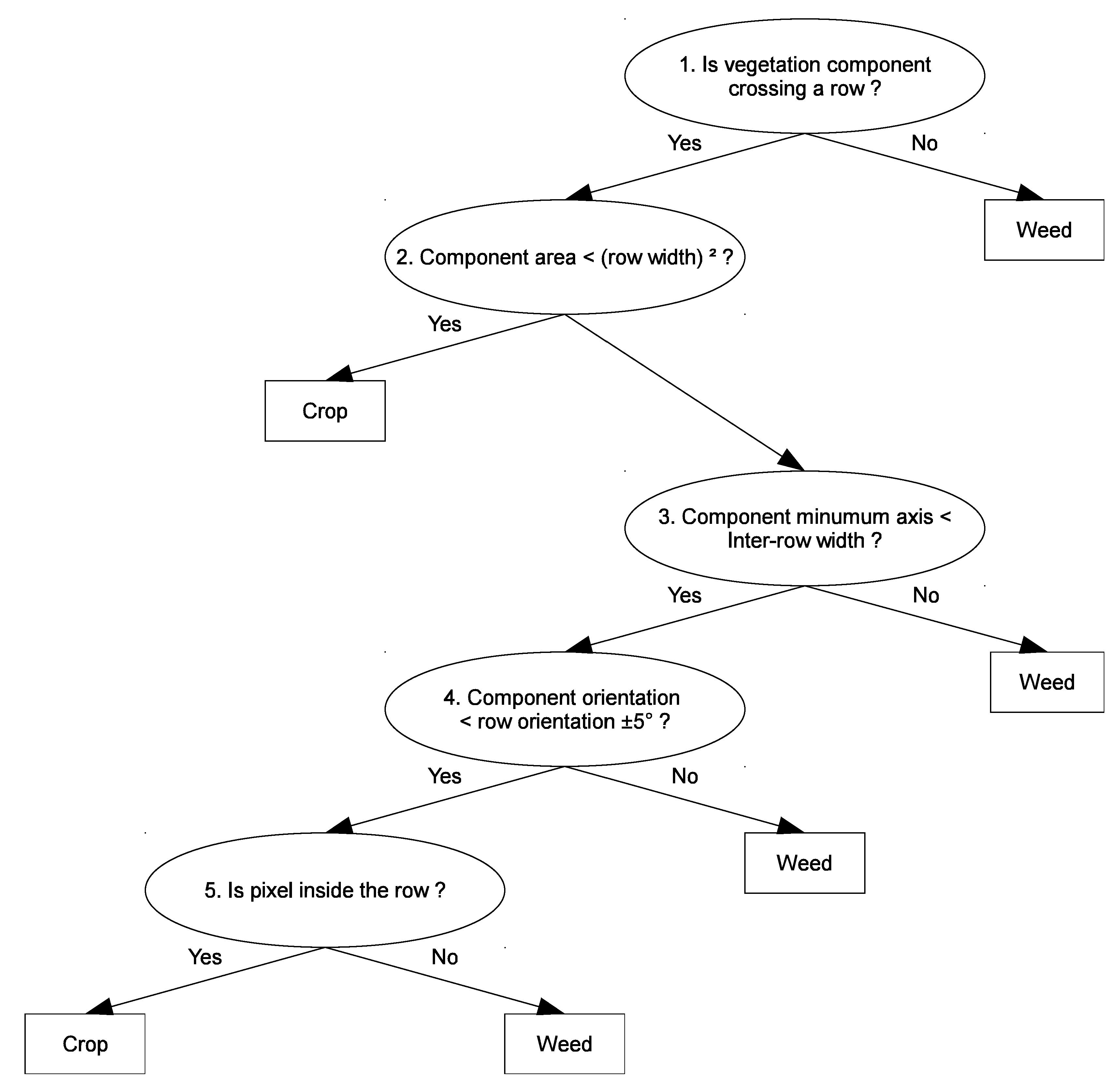
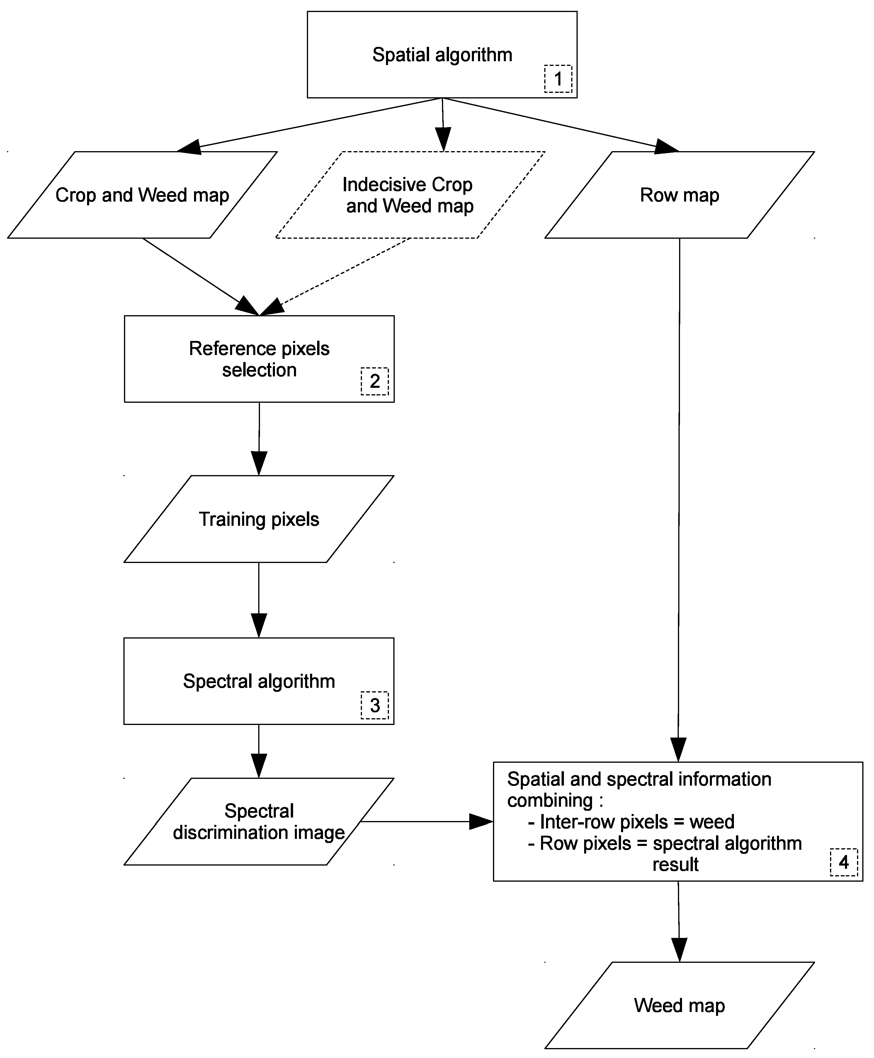
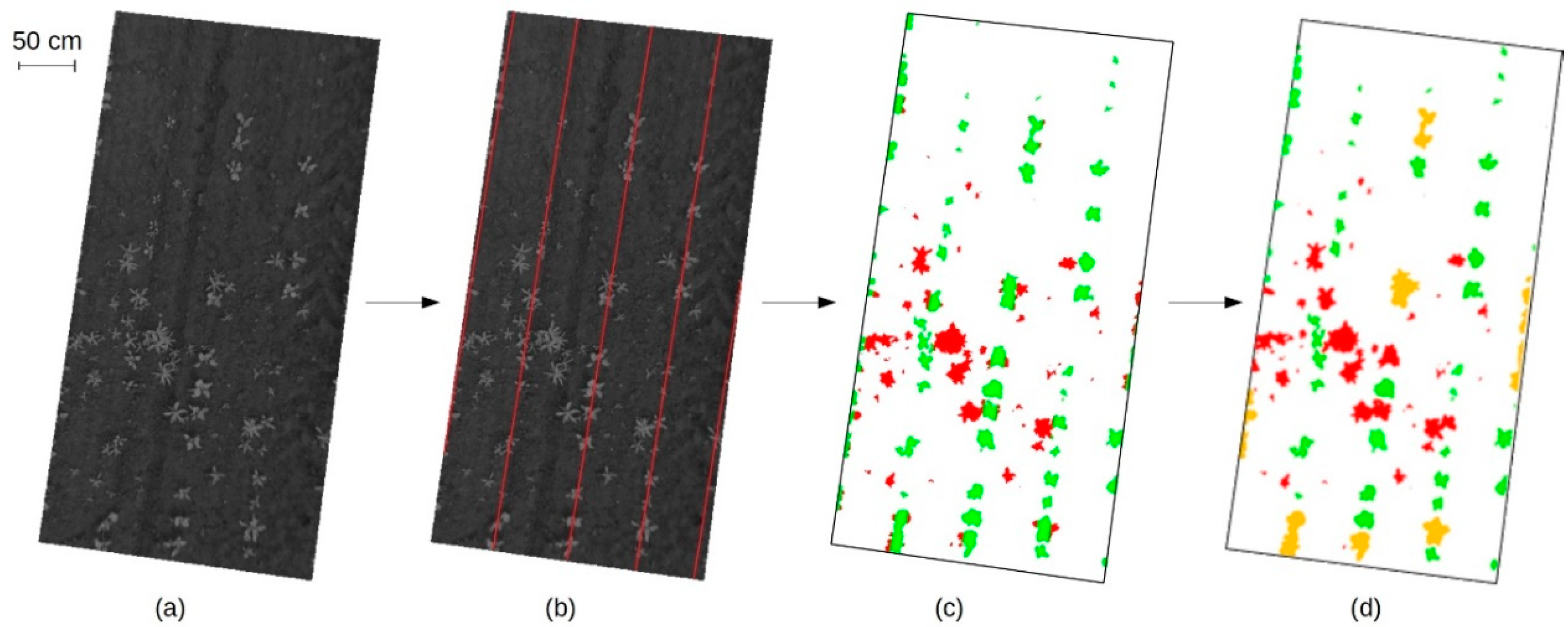
2.2.3. Weed Detection Procedure Combining Spatial and Spectral Methods

The spatial and spectral methods described in previous sections have specific limits: the first is not able to detect weed inside crop rows and the second requires manual supervision. A combination of these methods could overcome these limits and improve weed detection. This approach is based on two main assumptions: (1) Row is mostly crops and inter-row is mostly weeds and (2) The classification results obtained from the spatial method are accurate enough to be used as a training dataset. The procedure is described in Figure 7.
The first step in this procedure is the spatial method described in Section 2.2.1., it provides three images containing:
-
crop and weed map: pixels inside/outside of crop rows;
-
indecisive crop and weed map: pixels classified as crop or weed with less certainty, these results are obtained from step 3 to 5 described in Figure 4; and
-
row map.
The second step is to build the training dataset from the spatial method result: the training pixels are chosen from the crop and weed map (preferably) and from the indecisive crop and weed map (if there is not enough training pixels). This training dataset is built for each image (4 m × 3 m), taking into account the local specificity of both vegetation and image acquisition characteristics. The number of training pixels needed for each class is optimal at 200 (representing approximately 5 to 10% of total vegetation pixels), as discussed in [54]. The third step is the spectral method described in Section 2.2.2 with an automated training dataset. The forth step consolidates the results from spatial and spectral methods with a simple set of rules:
-
inter-row pixels are considered as weed (i.e., from spatial method) and
-
in-row pixel classes come from spectral method results.
At the end, the results are aggregated in a weed map.

2.2.4. Crop and Weed Detection Quality

To validate the developed algorithms, the number of pixels correctly classified was computed. Two indices were computed to assess the quality of classifications. First, the rate of crop pixels correctly classified was computed:
C = N u m b e r   o f   p i x e l s   o f   c r o p   c l a s s i f i e d   a s   c r o p T o t a l   n u m b e r   o f   p i x e l s   o f   c r o p .
Then, the rate of weed pixels correctly classified was computed:
W = N u m b e r   o f   p i x e l s   o f   w e e d   c l a s s i f i e d   a s   w e e d T o t a l   n u m b e r   o f   p i x e l s   o f   w e e d .
In the next section, the terms “crop detection rates” or “weed detection rates” represent a rate of pixels (of crop or weed) correctly classified.

3. Results and Discussion

To assess the contribution of the combination of spatial and spectral methods, three discrimination procedures were tested on 14 individual images (seven for sugar beet field and seven for maize field). First the spatial method (unsupervised) and the spectral method (supervised) were tested separately. Then an unsupervised method was proposed, based on the combination of spatial and spectral method. In this approach, the results of the spatial method were used as the training pixels for the classification of the spectral method.
The spatial algorithm was tested on multispectral images from both sugar beet and maize fields. The means of crop and weed detection rates ( μ C and μ W ) were computed on the 14 images. Results are presented in Table 1.
The spatial algorithm allows a good detection on crops, with a detection rate of 88% after having detected 100% of crop rows. In agreement with literature, spatial algorithms provided good results for crop rows detection. Peña, Torres-Sánchez, de Castro, Kelly and López-Granados [24] and López-Granados, Torres-Sánchez, Serrano-Pérez, de Castro, Mesas-Carrascosa and Peña [25] also detected 100% of crop rows in their images with the OBIA algorithm. On simulated images designed for algorithm assessment, they obtained the same results using an algorithm based on Hough transform. In the spatial algorithm presented in this study, the main errors of detection of crop pixels are due to the presence of weeds detected as crop in the row (Figure 8).
Concerning weed detection, the spatial algorithm correctly classified weed pixels with a rate of 0.79, which is close to literature results. For example, Peña, Torres-Sánchez, de Castro, Kelly and López-Granados [24] obtained an overall accuracy of 86% and Jones, et al. [55] correctly detected 75 to 91% of weeds. Weed pixels that were not correctly detected are mainly located in the rows.
Concerning the spectral algorithm, the classification procedure was repeated 10 times to minimize the impact of training pixel selection on the results. The means ( μ C and μ W ) of these repetitions were computed. Moreover, to compare the robustness of the classification methods and their repeatability, the standard deviations ( σ C and σ W ) of these indices were computed.
The spectral algorithm was tested on multispectral images of sugar beet and maize. Results are presented in Table 2 considering the SVM classification method.
The spectral algorithm used in this study obtained results close to literature, with a crop detection rate of 0.85 and a weed detection rate of 0.75. These results are in agreement with values obtained with spectral algorithms used on multi or hyperspectral images [56,57,58]. Piron, Leemans, Kleynen, Lebeau and Destain [58] correctly classified 66% of crops and 78% of weeds based on multispectral data. Other classifiers, such as linear discriminant analysis, applied on hyperspectral data discriminated correctly 91% of crops and 85% of weeds [56].
Looking at the image classification results (Figure 9), classification errors often occur for pixels located at plant edges. These pixels result from a spectral mixing of soil and vegetation, which decreases the quality of spectral information and thus the rate of good classification [44].
Concerning the spatial and spectral combination algorithm, the training pixels were automatically derived from the spatial method classification. Results are presented in Table 3.
As expected, the spatial and spectral combination improves weed detection, with an improved classification rate of 0.89 against 0.79 for the spatial method and 0.75 for the spectral method. This represents 10 to 14% of supplementary weed pixels that are correctly detected compared to the other methods. This is due to the better ability of spatial and spectral combination algorithm to detect weeds in the rows (using spectral information), as well as weeds outside the rows (using spatial information). Spatial and spectral combination results are illustrated in Figure 10.
Moreover, the range of weed detection rate standard deviation decreases from [0–0.14] for the repetitions of the spectral method to [0–0.06] for the combined algorithm. Thus, this algorithm not only improves the weed detection rate but also the detection robustness. Furthermore, this method is unsupervised, which allows automatic weed detection without any manual selection of training pixels.
Although our results have been compared with some of the literature, theses comparisons remain difficult, since data and validation methods are different. In terms of results, the spatial and spectral methods assessed in this study are similar to those encountered in the literature. Using multispectral images, this study demonstrates that combining spatial and spectral methods improves weed detection and its robustness.
In this paper, the validation method is based on the rate of pixels correctly classified and not on the rate of plants. The rate of pixels can be directly linked to the rate of infested areas, which is interesting information for precision spraying, such as allowing farmers to anticipate the surface to be sprayed. The classification quality was analyzed using two indices (crop and weed detection rate) which are part of the confusion matrix. These indices were used (especially the weed detection rate) because of their agronomical significance. Considering the economic risk due to weed growth in commercial crops, the emphasis was put on weed detection. As the main objective is to control weeds, detecting crop as weed is less threatening than missing weed.
The originality of this study is to combine the advantages of spatial and spectral methods and to transform a supervised method into an unsupervised one. This work can be compared to two recent studies which also aim to develop unsupervised detection approaches. Compared to Gao, Liao, Nuyttens, Lootens, Vangeyte, Pižurica, He and Pieters [42] our approach uses NIR information which helps in improving vegetation discrimination as suggested by [42]. Moreover, the training dataset building is fully automatic for crop and weeds while it automatic only for weeds in [42]. The method developed in this paper only uses four-band images and do not require any additional information such as 3D data or Digital Surface Models [43]. The development of such unsupervised algorithms allows detecting weeds automatically without previous selection of training data, reducing human and economic costs. This not only avoids operator bias but also circumvents difficulties to manage image variabilities. In our method, the automatic selection of training pixels provides a specific training set for each image, managing the variability observed in the fields (e.g., soil color, plant stress, growth stage) and due to acquisition conditions (e.g., luminosity, shadows).
This procedure has been developed independently from the acquisition vehicle and could be used to detect weeds using UAV or UGV (Unmanned Ground Vehicle). The spatial resolution should be at least of 6 mm/pix and the pixel number of the sensor should be chosen to obtain this resolution regarding its acquisition height. In case of non-vertical view axis, additional difficulties may arise regarding geometrical image distortion (e.g., presence of perspective and variable spatial resolution). Disregarding these requirements or difficulties, UAV or UGV could prove useful to acquire images on whole fields and build weed maps.
In terms of applicability, the algorithms developed in this paper and in [42,43] are proved to work on wide-row crops (i.e., maize and sugar beet in this study, sunflower and cotton in [43], maize in [42]). At the present time, these approaches are not adapted to narrow-row crops since their algorithms require the identification of inter-row area.
To go on with this study, the impact of the selection of the training pixels on the spectral classification could be assessed. Indeed, training pixels are selected from the results of the spatial detection, where classification errors can occur. In this paper, the spatial method is considered as reliable. Thus, it should be interesting to test different error levels in the training pixels to assess its impact on the spatial and spectral combination algorithm robustness. Moreover, different methods could be tested to select the best training pixels.

4. Conclusions

The main objective of this paper was to develop an unsupervised image processing algorithm to detect weeds in crop rows without human intervention. This objective is fulfilled with the development of a classification algorithm using results from a spatial based method to automatically create a training dataset used to discriminate crop from weeds using their spectral signatures. The spatial approach (Hough Transform) is used to detect crop rows and to build a training dataset with the assumption that most of the crops are located in the rows and most of the weeds are outside the rows. The resulting training dataset allows an automated spectral classification (SVM) on the pixels located in the crop rows to improve weed detection rate. The resulting classification is a combination of the results obtained by both approaches.
This algorithm has been assessed and offers results similar to those found in the literature with the major benefit of being unsupervised. The combination of spatial and spectral information improves weed detection rate as well as the robustness of the overall classification. Not only reducing operator bias, this automation also implies a greater adaptability as the training dataset is computed for each image, taking its specificities (such as plant growth stages, lighting condition, soil color, etc.) into account.
Images used in this paper were acquired with a camera mounted on a pole but the resulting spatial resolutions could be obtained with an Unmanned Terrestrial Vehicle or an Unmanned Aerial Vehicle using a higher resolution sensor and/or flying at a low altitude. Another perspective to further improve the detection rate and classification robustness lies in the use of other kinds of information (such as plant morphology or leaves texture) to build the result.
This work is part of the development of weed detection devices that are of particular interest to reach the challenge of site specific weed management using chemical or physical actions.

Author Contributions

M.L., G.J., S.V., C.G., and R.F. conceived and designed the experiments; M.L. performed the experiments and analyzed the data; G.J., S.V., C.G., R.F., J.-N.P., and T.M. contributed materials and analysis tools; M.L., G.J., S.V., and C.G. wrote the paper.

Funding

This study is supported by the program ‘‘ANR CoSAC’’ (ANR-14-CE18-0007) and the Horizon 2020 project IWMPRAISE (grant agreement No. 727321).

Acknowledgements

This project is supported by AIRINOV Company and the ANRT (Association Nationale de la Recherche et de la Technologie).

Conflicts of Interest

The authors declare no conflict of interest.

References

  1. Oerke, E. Crop losses to pests. J. Agric. Sci. 2006, 144, 31–43. [Google Scholar] [CrossRef]
  2. Timmermann, C.; Gerhards, R.; Kühbauch, W. The economic impact of site-specific weed control. Precis. Agric. 2003, 4, 249–260. [Google Scholar] [CrossRef]
  3. Weis, M.; Gutjahr, C.; Ayala, V.R.; Gerhards, R.; Ritter, C.; Schölderle, F. Precision farming for weed management: Techniques. Gesunde Pflanzen 2008, 60, 171–181. [Google Scholar] [CrossRef]
  4. Lee, W.S.; Slaughter, D.; Giles, D. Robotic weed control system for tomatoes. Precis. Agric. 1999, 1, 95–113. [Google Scholar] [CrossRef]
  5. Gerhards, R.; Oebel, H. Practical experiences with a system for site-specific weed control in arable crops using real-time image analysis and GPS-controlled patch spraying. Weed Res. 2006, 46, 185–193. [Google Scholar] [CrossRef]
  6. Stafford, J.V.; Ambler, B. In-field location using GPS for spatially variable field operations. Comput. Electron. Agric. 1994, 11, 23–36. [Google Scholar] [CrossRef]
  7. Nordmeyer, H. Patchy weed distribution and site-specific weed control in winter cereals. Precis. Agric. 2006, 7, 219–231. [Google Scholar] [CrossRef]
  8. Gutjahr, C.; Sokefeld, M.; Gerhards, R. Evaluation of two patch spraying systems in winter wheat and maize. Weed Res. 2012, 52, 510–519. [Google Scholar] [CrossRef]
  9. Riemens, M. Developments in physical weed control in northwest Europe. Julius-Kühn-Archiv 2016, 24, 24–26. [Google Scholar]
  10. Zhang, C.; Kovacs, J.M. The application of small unmanned aerial systems for precision agriculture: A review. Precis. Agric. 2012, 13, 693–712. [Google Scholar] [CrossRef]
  11. Rasmussen, J.; Nielsen, J.; Garcia-Ruiz, F.; Christensen, S.; Streibig, J.C. Potential uses of small unmanned aircraft systems (UAS) in weed research. Weed Res. 2013, 53, 242–248. [Google Scholar] [CrossRef]
  12. Lamb, D.W.; Brown, R.B. Remote-sensing and mapping of weeds in crops. J. Agric. Eng. Res. 2001, 78, 117–125. [Google Scholar] [CrossRef]
  13. Herrmann, I.; Shapira, U.; Kinast, S.; Karnieli, A.; Bonfil, D. Ground-level hyperspectral imagery for detecting weeds in wheat fields. Precis. Agric. 2013, 14, 637–659. [Google Scholar] [CrossRef]
  14. Shapira, U.; Herrmann, I.; Karnieli, A.; Bonfil, D.J. Field spectroscopy for weed detection in wheat and chickpea fields. Int. J. Remote Sens. 2013, 34, 6094–6108. [Google Scholar] [CrossRef]
  15. Huang, Y.; Lee, M.A.; Thomson, S.J.; Reddy, K.N. Ground-based hyperspectral remote sensing for weed management in crop production. Int. J. Agric. Biol. Eng. 2016, 9, 98. [Google Scholar]
  16. Feyaerts, F.; Van Gool, L. Multi-spectral vision system for weed detection. Pattern Recognit. Lett. 2001, 22, 667–674. [Google Scholar] [CrossRef]
  17. Vrindts, E.; De Baerdemaeker, J.; Ramon, H. Weed detection using canopy reflection. Precis. Agric. 2002, 3, 63–80. [Google Scholar] [CrossRef]
  18. Girma, K.; Mosali, J.; Raun, W.; Freeman, K.; Martin, K.; Solie, J.; Stone, M. Identification of optical spectral signatures for detecting cheat and ryegrass in winter wheat. Crop Sci. 2005, 45, 477–485. [Google Scholar] [CrossRef]
  19. Carter, G.A.; Knapp, A.K. Leaf optical properties in higher plants: Linking spectral characteristics to stress and chlorophyll concentration. Am. J. Bot. 2001, 88, 677–684. [Google Scholar] [CrossRef] [PubMed]
  20. Torres-Sánchez, J.; López-Granados, F.; De Castro, A.I.; Peña-Barragán, J.M. Configuration and specifications of an unmanned aerial vehicle (UAV) for early site specific weed management. PLoS ONE 2013, 8, e58210. [Google Scholar] [CrossRef] [PubMed]
  21. Peña, J.M.; Torres-Sánchez, J.; Serrano-Pérez, A.; de Castro, A.I.; López-Granados, F. Quantifying efficacy and limits of unmanned aerial vehicle (UAV) technology for weed seedling detection as affected by sensor resolution. Sensors 2015, 15, 5609–5626. [Google Scholar] [CrossRef] [PubMed]
  22. Lottes, P.; Khanna, R.; Pfeifer, J.; Siegwart, R.; Stachniss, C. UAV-based crop and weed classification for smart farming. In Proceedings of the IEEE International Conference on Robotics and Automation (ICRA), Singapore, 29 May–3 June 2017. [Google Scholar]
  23. Pérez-Ortiz, M.; Peña, J.M.; Gutiérrez, P.A.; Torres-Sánchez, J.; Hervás-Martínez, C.; López-Granados, F. Selecting patterns and features for between-and within-crop-row weed mapping using UAV-imagery. Expert Syst. Appl. 2016, 47, 85–94. [Google Scholar] [CrossRef]
  24. Peña, J.M.; Torres-Sánchez, J.; de Castro, A.I.; Kelly, M.; López-Granados, F. Weed mapping in early-season maize fields using object-based analysis of unmanned aerial vehicle (UAV) images. PLoS ONE 2013, 8, e77151. [Google Scholar] [CrossRef] [PubMed]
  25. López-Granados, F.; Torres-Sánchez, J.; Serrano-Pérez, A.; de Castro, A.I.; Mesas-Carrascosa, F.J.; Peña, J.-M. Early season weed mapping in sunflower using UAV technology: Variability of herbicide treatment maps against weed thresholds. Precis. Agric. 2016, 17, 183–199. [Google Scholar] [CrossRef]
  26. Rouse, J.; Haas, R.; Schell, J.; Deering, D. Monitoring vegetation systems in the Great Plains with ERTS. In Third Earth Resources Technology Satellite-1 Symposium—Volume I: Technical Presentations; NASA: Washington, DC, USA, 1974; p. 309. [Google Scholar]
  27. Woebbecke, D.M.; Meyer, G.E.; Von Bargen, K.; Mortensen, D.A. Color indices for weed identification under various soil, residue, and lighting conditions. Trans. ASAE 1995, 38, 259–269. [Google Scholar] [CrossRef]
  28. Torres-Sánchez, J.; Peña, J.; de Castro, A.; López-Granados, F. Multi-temporal mapping of the vegetation fraction in early-season wheat fields using images from UAV. Comput. Electron. Agric. 2014, 103, 104–113. [Google Scholar] [CrossRef]
  29. Torres-Sánchez, J.; López-Granados, F.; Peña, J.M. An automatic object-based method for optimal thresholding in UAV images: Application for vegetation detection in herbaceous crops. Comput. Electron. Agric. 2015, 114, 43–52. [Google Scholar] [CrossRef]
  30. Ahmed, F.; Al-Mamun, H.A.; Bari, A.S.M.H.; Hossain, E.; Kwan, P. Classification of crops and weeds from digital images: A support vector machine approach. Crop Prot. 2012, 40, 98–104. [Google Scholar] [CrossRef]
  31. Pérez, A.J.; López, F.; Benlloch, J.V.; Christensen, S. Colour and shape analysis techniques for weed detection in cereal fields. Comput. Electron. Agric. 2000, 25, 197–212. [Google Scholar] [CrossRef]
  32. Burks, T.; Shearer, S.; Payne, F. Classification of weed species using color texture features and discriminant analysis. Trans. ASAE 2000, 43, 441. [Google Scholar] [CrossRef]
  33. Marchant, J.A. Tracking of row structure in three crops using image analysis. Comput. Electron. Agric. 1996, 15, 161–179. [Google Scholar] [CrossRef]
  34. Leemans, V.; Destain, M.F. Application of the hough transform for seed row localisation using machine vision. Biosyst. Eng. 2006, 94, 325–336. [Google Scholar] [CrossRef]
  35. Tillett, N.D.; Hague, T.; Miles, S.J. Inter-row vision guidance for mechanical weed control in sugar beet. Comput. Electron. Agric. 2002, 33, 163–177. [Google Scholar] [CrossRef]
  36. Hague, T.; Tillett, N.D.; Wheeler, H. Automated crop and weed monitoring in widely spaced cereals. Precis. Agric. 2006, 7, 21–32. [Google Scholar] [CrossRef]
  37. Vioix, J.-B.; Douzals, J.-P.; Truchetet, F.; Assémat, L.; Guillemin, J.-P. Spatial and spectral methods for weed detection and localization. EURASIP J. Adv. Signal Proc. 2002, 2002, 793080. [Google Scholar] [CrossRef]
  38. Gabor, D. Theory of communication. Part 1: The analysis of information. Electr. Eng. Part III Radio Commun. Eng. J. Inst. 1946, 93, 429–441. [Google Scholar] [CrossRef]
  39. Vioix, J.-B. Conception et Réalisation d’un Dispositif D’imagerie Multispectrale Embarqué: Du Capteur aux Traitements Pour la Détection D’adventices. Ph.D. Thesis, Université de Bourgogne, Dijon, France, 2004. [Google Scholar]
  40. Hung, C.; Xu, Z.; Sukkarieh, S. Feature learning based approach for weed classification using high resolution aerial images from a digital camera mounted on a UAV. Remote Sens. 2014, 6, 12037. [Google Scholar] [CrossRef]
  41. Pérez-Ortiz, M.; Gutiérrez, P.A.; Peña, J.M.; Torres-Sánchez, J.; Hervás-Martínez, C.; López-Granados, F. An experimental comparison for the identification of weeds in sunflower crops via unmanned aerial vehicles and object-based analysis. In Proceedings of the International Work-Conference on Artificial Neural Networks, Palma de Mallorca, Spain, 10–12 June 2015; Springer: Berlin, Germany, 2015; pp. 252–262. [Google Scholar]
  42. Gao, J.; Liao, W.; Nuyttens, D.; Lootens, P.; Vangeyte, J.; Pižurica, A.; He, Y.; Pieters, J.G. Fusion of pixel and object-based features for weed mapping using unmanned aerial vehicle imagery. Int. J. Appl. Earth Obs. Geoinform. 2018, 67, 43–53. [Google Scholar] [CrossRef]
  43. De Castro, A.; Torres-Sánchez, J.; Peña, J.; Jiménez-Brenes, F.; Csillik, O.; López-Granados, F. An automatic random forest-obia algorithm for early weed mapping between and within crop rows using UAV imagery. Remote Sens. 2018, 10, 285. [Google Scholar] [CrossRef]
  44. Louargant, M.; Villette, S.; Jones, G.; Vigneau, N.; Paoli, J.N.; Gée, C. Weed detection by UAV: Simulation of the impact of spectral mixing in multispectral images. Precis. Agric. 2017, 18, 932–951. [Google Scholar] [CrossRef]
  45. Meier, U. Growth Stages of Mono- and Dicotyledonous Plants; Blackwell Wissenschafts-Verlag: Berlin, Germany, 1997. [Google Scholar]
  46. Verger, A.; Vigneau, N.; Chéron, C.; Gilliot, J.-M.; Comar, A.; Baret, F. Green area index from an unmanned aerial system over wheat and rapeseed crops. Remote Sens. Environ. 2014, 152, 654–664. [Google Scholar] [CrossRef]
  47. Gonzalez, R.C.; Woods, R.E. Introduction to the fourier transform and the frequency domain. In Digital Image Processing, 2nd ed.; Prentice Hall: Upper Saddle River, NJ, USA, 2002; pp. 149–167. [Google Scholar]
  48. Tucker, C.J. Red and photographic infrared linear combinations for monitoring vegetation. Remote Sens. Environ. 1979, 8, 127–150. [Google Scholar] [CrossRef]
  49. Rouse, J.W., Jr.; Haas, R.; Schell, J.; Deering, D. Monitoring vegetation systems in the great plains with erts. In Goddard Space Flight Center 3d ERTS-1 Symposium; NASA: Washington, DC, USA, 1974; Volume 1, pp. 309–317. [Google Scholar]
  50. Otsu, N. A threshold selection method from gray-level histograms. IEEE Trans. Syst. Man Cybern. 1979, 9, 62–66. [Google Scholar] [CrossRef]
  51. Hough, P.V.C. Method and Means for Recognizing Complex Patterns. U.S. Patent 3,069,654, 18 December 1962. [Google Scholar]
  52. Duda, R.O.; Hart, P.E. Use of the hough transformation to detect lines and curves in pictures. Commun. Assoc. Comput. Mach. 1972, 15, 11–15. [Google Scholar] [CrossRef]
  53. Pérez-Ortiz, M.; Peña, J.M.; Gutiérrez, P.A.; Torres-Sánchez, J.; Hervás-Martínez, C.; López-Granados, F. A semi-supervised system for weed mapping in sunflower crops using unmanned aerial vehicles and a crop row detection method. Appl. Soft Comput. 2015, 37, 533–544. [Google Scholar] [CrossRef]
  54. Louargant, M. Proxidétection des Adventices par Imagerie Aérienne: Vers un Service de Gestion par Drone. Ph.D. Thesis, Université de Bourgogne, Dijon, France, 2016. [Google Scholar]
  55. Jones, G.; Gée, C.; Truchetet, F. Assessment of an inter-row weed infestation rate on simulated agronomic images. Comput. Electron. Agric. 2009, 67, 43–50. [Google Scholar] [CrossRef]
  56. Hadoux, X.; Gorretta, N.; Rabatel, G. Weeds-wheat discrimination using hyperspectral imagery. In Proceedings of the International Conference on Agricultural Engineering, Valence, Spain, 8–12 July 2012. [Google Scholar]
  57. Borregaard, T.; Nielsen, H.; Norgaard, L.; Have, H. Crop-weed discrimination by line imaging spectroscopy. J. Agric. Eng. Res. 2000, 75, 389–400. [Google Scholar] [CrossRef]
  58. Piron, A.; Leemans, V.; Kleynen, O.; Lebeau, F.; Destain, M.F. Selection of the most efficient wavelength bands for discriminating weeds from crop. Comput. Electron. Agric. 2008, 62, 141–148. [Google Scholar] [CrossRef]
Figure 1. The ground multispectral imaging system fixed on a pole for the acquisition of high spatial resolution image (6 mm/pixel).
Remotesensing 10 00761 g001
Figure 2. Transmittance of the filters (a) and sensitivity curve of the sensors (b) from multiSPEC 4C producer datasheet.
Remotesensing 10 00761 g002
Figure 3. Spatial method procedure from original image to weed map.
Remotesensing 10 00761 g003
Figure 4. Decision tree applied on each connected component to discriminate crop from weeds using detected rows and shape analysis.
Remotesensing 10 00761 g004
Figure 5. Spectral method procedure from original image to weed map.
Remotesensing 10 00761 g005
Figure 6. Image processing steps to estimate the vegetation rate from a Normalized Difference Vegetation Index (NDVI) image with a 6 mm spatial resolution. (a) NDVI image (the color scale reflects NDVI from 0.1 to 0.7); (b) Connected components image after threshold (soil in black and vegetation in white); and (c) Vegetation rate estimation from 0 (black) to 1 (white).
Remotesensing 10 00761 g006
Figure 7. Combination of spatial and spectral information from original image to weed map.
Remotesensing 10 00761 g007
Figure 8. Example of the spatial algorithm results. (a) Multispectral orthoimage; (b) Row location (row axis in red); (c) Weed location (crop in green, weed in red); (d) Classification of the connected components on the rows (crop in green, weed in red, unknown class in orange).
Remotesensing 10 00761 g008
Figure 9. Example of the spectral algorithm results. (a) Multispectral orthoimage; (b) Crop (green) and weed (red) location.
Remotesensing 10 00761 g009
Figure 10. Example of the spatial and spectral combination results using an SVM classifier. (a) Multispectral orthoimage; (b) Crop (green) and weed (red) location deduced from spatial information; (c) Weed (green) and crop (red) location deduced from spectral information; (d) Weed (green) and crop (red) location deduced from the combination of spatial and spectral information.
Remotesensing 10 00761 g010
Table 1. Results of the spatial algorithm; μ C is the mean of crop detection rates, μ W is the mean of weed detection rates computed on the 14 images of sugar beet and maize fields.
Situations μ C μ W
Results on images of sugar beet field0.890.74
Results on images of maize field0.860.84
Results on all images0.880.79
Table 2. Results of the spectral algorithm; μ C is the mean of crop detection rates, μ W is the mean of weed detection rates computed on the 14 images of sugar beet and maize fields. [ σ C m i n σ C m a x ] is the min-max interval of the standard deviations of crops correctly classified, computed on 10 repetitions for each image. [ σ C m i n σ C m a x ] is defined similarly for weeds.
Situations μ C μ W [ σ C m i n σ C m a x ][ σ W m i n σ W m a x ]
Results on images of sugar beet field 0.940.67[0.01–0.09][0.02–0.14]
Results on images of maize field 0.760.83[0.01–0.05][0–0.06]
Results on all images0.850.75[0.01–0.09][0–0.14]
Table 3. Results comparison of the spatial and spectral algorithms; μ C is the mean of rates of crops correctly classified, μ A is the mean of rates of weeds correctly classified. [ σ C m i n σ C m a x ] is the min-max interval of the standard deviations of crops correctly classified, computed on 10 repetitions for each image. [ σ W m i n σ W m a x ] is defined similarly for weeds.
Situations μ C μ W [ σ C m i n σ C m a x ][ σ W m i n σ W m a x ]
Results on images of sugar beet field0.920.81[0.01–0.04][0–0.06]
Results on images of maize field0.740.97[0.02–0.04][0–0.01]
Results on all images0.830.89[0.01–0.04][0–0.06]

