Field-Scale Assessment of Land and Water Use Change over the California Delta Using Remote Sensing

Abstract

The ability to accurately monitor and anticipate changes in consumptive water use associated with changing land use and land management is critical to developing sustainable water management strategies in water-limited climatic regions. In this paper, we present an application of a remote sensing data fusion technique for developing high spatiotemporal resolution maps of evapotranspiration (ET) at scales that can be associated with changes in land use. The fusion approach combines ET map timeseries developed using an multi-scale energy balance algorithm applied to thermal data from Earth observation platforms with high spatial but low temporal resolution (e.g., Landsat) and with moderate resolution but frequent temporal coverage (e.g., MODIS (Moderate Resolution Imaging Spectroradiometer)). The approach is applied over the Sacramento-San Joaquin Delta region in California—an area critical to both agricultural production and drinking water supply within the state that has recently experienced stresses on water resources due to a multi-year (2012–2017) extreme drought. ET “datacubes” with 30-m resolution and daily timesteps were constructed for the 2015–2016 water years and related to detailed maps of land use developed at the same spatial scale. The ET retrievals are evaluated at flux sites over multiple land covers to establish a metric of accuracy in the annual water use estimates, yielding root-mean-square errors of 1.0, 0.8, and 0.3 mm day⁻¹ at daily, monthly, and yearly timesteps, respectively, for all sites combined. Annual ET averaged over the Delta changed only 3 mm year⁻¹ between water years, from 822 to 819 mm year⁻¹, translating to an area-integrated total change in consumptive water use of seven thousand acre-feet (TAF). Changes were largest in areas with recorded land-use change between water years—most significantly, fallowing of crop land presumably in response to reductions in water availability and allocations due to the drought. Moreover, the time evolution in water use associated with wetland restoration—an effort aimed at reducing subsidence and carbon emissions within the inner Delta—is assessed using a sample wetland chronosequence. Region-specific matrices of consumptive water use associated with land use changes may be an effective tool for policymakers and farmers to understand how land use conversion could impact consumptive use and demand.

1. Introduction

Across the United States and globally there are ever increasing and competing demands for freshwater resources for use in agriculture, ecosystem support, industry, and urban development. Recent extended droughts in the western and southeastern U.S. have exacerbated ongoing inter-state “water wars”, with regional conditions anticipated to further dry as the climate continues to change [1,2]. Studies using the Gravity Recovery and Climate Experiment (GRACE) satellite have identified severely stressed major aquifers around the globe that are being unsustainably depleted due to over-abstraction, primarily in support of irrigated agriculture [3,4]. To facilitate wise water management, and to develop sustainable agricultural systems that will feed the Earth’s growing population into the future, there is a critical need for robust assessments of consumptive water use, or evapotranspiration (ET), at the scale of anthropogenic activity. Furthermore, we must better understand how changes in land use and land management relate to changes in water use and supply, including surface and groundwater resources.

The Central Valley Aquifer system in California was identified in GRACE experiments as extremely variably stressed, meaning there is some potential for recharge but extraction far exceeds recharge rates on average [3]. This aquifer underlies a water-limited agricultural production area and supports widespread irrigation, exploiting the long growing season and plentiful sunshine that is characteristic of this region. Water supplies for irrigation are drawn from a combination of surface and groundwater sources, supported by runoff from snowpack in the Sierra Nevada mountain range. GRACE-based trend analyses of groundwater storage in the Sacramento-San Joaquin River basin indicate an annual aquifer depletion rate of −20 mm year⁻¹ for the period 2003–2010, with higher rates during drought years when groundwater pumping increases to counterbalance limited surface water supplies [5]. Dropping water tables resulting from extensive groundwater withdrawals have led to major land subsidence in many parts of the Central Valley over the past decades [6], with some localized areas subsiding 0.5 m year⁻¹ during the latter part of the most recent multi-year California drought (2012–2017) [7]. High rates of subsidence are often associated with areas measuring historically low water table levels where perennial crops (vineyards and orchards) are replacing non-permanent field crops and pastures, effectively “hardening demand” for water use [8].

Water use, groundwater storage and land use are strongly coupled in the Central Valley—particularly during periods of drought. Possible grower responses to surface water allocation limitations include shifts from surface to groundwater supplies, adoption of more efficient irrigation strategies, fallowing of fields, and conversion to crops with lower water requirements. Economics also play a role [9]. For example, as wells dewatered during the 2012–2017 drought, growers with sufficient financial resources could drill deeper wells to sustain production, while other farmers could not afford the added expense. Improving our understanding of potential response to limited water supply is critical to the long-term sustainability of this agricultural production system.

This study describes an approach for operational accounting of water usage by landcover type and water management strategy, with a geographic focus on the Sacramento-San Joaquin Delta region of California. The Delta serves as the hub of the California water supply system, channeling about half the state’s total runoff and providing drinking water for 23 million people and irrigation water for agricultural acreage across the San Joaquin valley [10,11,12]. However, a combination of anthropogenic and natural stressors has led to a general decline in ecosystem health and reliability of water supply [13]. In 2014, the State Water Resources Control Board’s Office of the Delta Watermaster commissioned an ET model intercomparison study [14] to evaluate current capabilities for water accounting in support of the California Sustainable Groundwater Management Act (SGMA). This act obligates authorities in medium and high priority groundwater basins within the state to prepare and implement long-term groundwater management plans, with the Delta designated as a high priority basin for SGMA planning. Accurate maps of ET developed at sub-field scales were identified as a key tool in this endeavor.

The Delta is also the focus of a major wetland restoration project aimed at rebuilding soil organic carbon stores that have been lost through oxidation in lands that have been drained for agricultural production. The Delta has subsided in some places up to 8 m, imposing threats regarding levee failure and water quality/saltwater intrusion [15]. The goal of the restoration project is to reverse subsidence in the Delta region while at the same time to increase carbon sinks by building up organic matter through conversion of dry land agricultural fields to wetlands and rice cultivation [11,12,16]. These land-use changes have the potential to significantly impact the local climate and water balance. Baldocchi et al. [17], for example, conclude that expansion of flooded rice acreage and wetlands can also have a feedback on local atmospheric conditions, serving to humidify the surface layer and reduce evaporative demand. Here, too, spatially explicit timeseries maps of ET developed at the scale of restoration activities will provide information required for quantifying feedbacks to the local and regional hydrology and climate.

Ideally, the ET mapping algorithms used would require minimal a priori information regarding crop condition and management practices, as these are precisely the types of behaviors we wish to investigate. Standard water balance and crop coefficient approaches for ET estimation generally assume optimal crop conditions and irrigation strategies, and may overestimate actual crop ET under water limited conditions. In contrast, satellite remote sensing methods based on surface energy balance, using thermal infrared (TIR) retrievals of land-surface temperature (LST), have demonstrated utility for determining surface moisture status and actual evaporative fluxes given little prior knowledge of the system [18]. The LST inputs are used to effectively “diagnose” water use patterns over the landscape, although ancillary information may be required to interpret these patterns.

To map water use at the scale of management requires relatively high resolution thermal satellite imagery. Based on analyses presented by Yan and Roy [19], the average field size in the CA Central Valley is 0.234 km², or approximately 500 × 500 m (Yan, 2017, personal comm.). Satellite-based ET retrievals at 100-m resolution or finer enable mapping at these critical spatial scales, allowing sub-field sampling and exclusion of border pixels in most fields. Routine, global TIR imaging at the 100-m scale is currently supported only by the Landsat satellites, with a long-term archive back to the 1980s.The temporal revisit of Landsat (16 days for a single platform), however, has proven to be a limiting factor in accurately retrieving seasonal water use estimates in regions with moderate to pervasive cloud cover climatologies. For such regions, a data fusion methodology can be employed to fuse high-spatial/low-temporal resolution (e.g., Landsat) ET retrievals with ET derived from moderate-spatial (1 km)/high-temporal (daily) resolution TIR sensors (e.g., the Moderate Resolution Imaging Spectroradiometer; MODIS). The end products are ET datacubes with both high spatial (30 m) and temporal (daily) resolution [20]. This data fusion technique was included in the Delta ET intercomparison study as a potential method for routine water use accounting [14]. It is also being leveraged to provide information for vineyard irrigation management in California under the Grape Remote sensing Atmospheric Profile and Evapotranspiration eXperiment (GRAPEX) [21]. The method has potential for wetland restoration studies as well, providing estimates of evaporative fluxes at scales resolving individual management units.

In this study, we look in depth at an E0T datacube generated for the 2015–2016 water years over the California Delta region and its utility for providing actionable information regarding field-scale water use estimates. A primary goal of the study is to develop accuracy metrics for daily to annual water use estimates using micrometeorological data from a suite of eddy covariance flux towers operating within the modeling domain, sampling a subset of the diverse vegetation that characterize the region. In particular, performance is evaluated over restored wetland sites where energy balance can be significantly modified by the water substrate. The ET datacube is then used to investigate changes in water use in response to land use and land/water management changes that occurred between years, in part in response to the long-term drought conditions and resulting water limitations. Practical challenges for supporting operational management applications are also discussed.

2. Materials and Methods

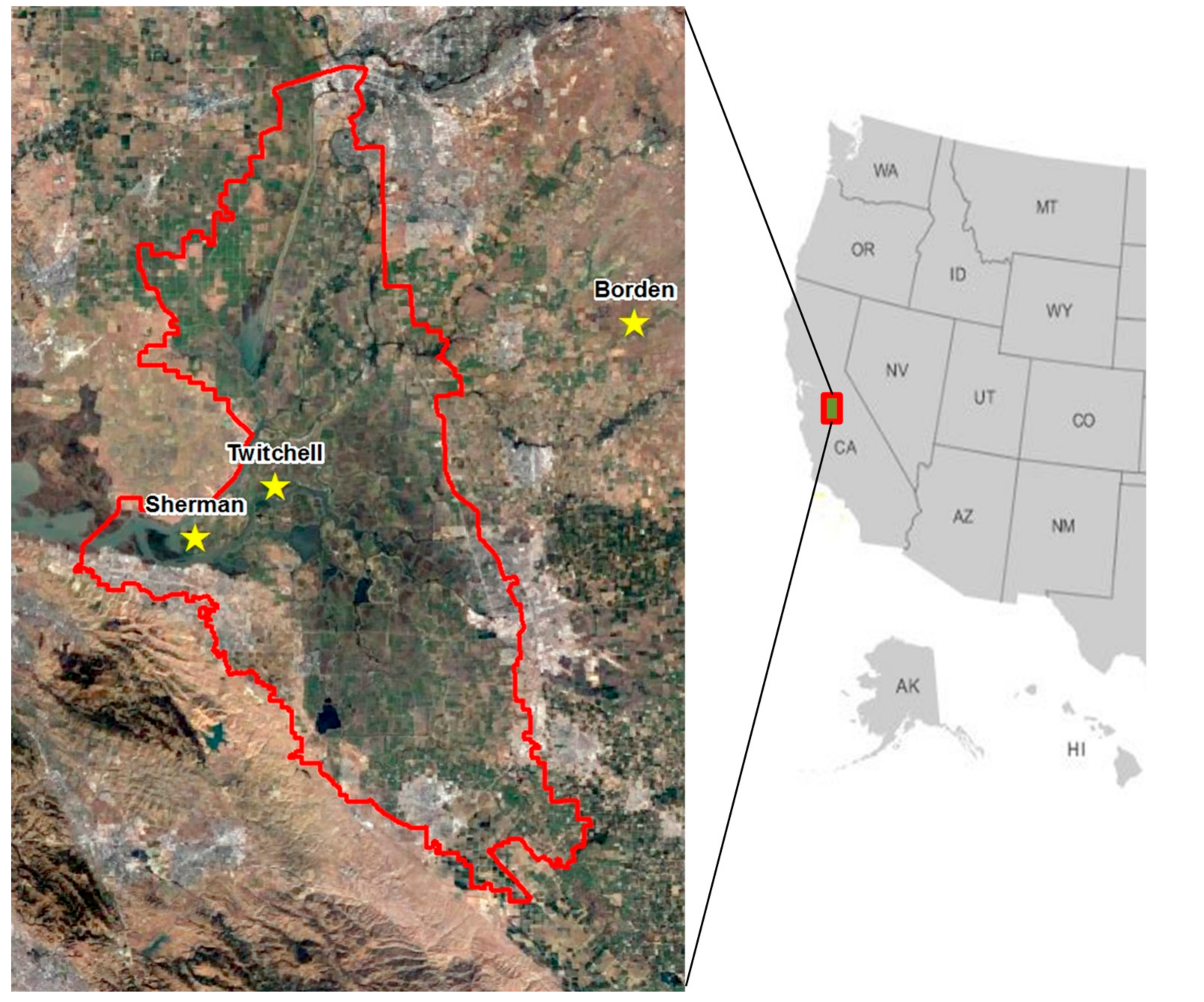
2.1. Study Domain

The study domain is shown in Figure 1, along with a delimitation of the Legal Delta boundaries as defined by the 1959 Delta Protection Act. The Delta contains the confluence of the Sacramento and San Joaquin Rivers and serves as a major hub for water supply within the state of California. Rich in sediment and peat soils developed over years of deposition and decomposition of wetland vegetation, the region was largely drained and leveed in support of agriculture in the late 1800s. Exposure of the peat organic matter to air resulted in oxidation of the soils, compaction, and wind erosion, all leading to subsidence, with some areas now 7–8 m below sea level. Wetland restoration activities, and conversion of dryland agriculture to flooded rice production, are aimed at rebuilding the organic soils and reducing subsidence and CO₂ emissions caused by oxidation. Restored wetlands have been established on leveed islands in the central and western Delta, specifically Sherman and Twitchell Islands. Several flux towers are deployed on these islands to monitor water and carbon fluxes from a chronosequence of restored wetlands and converted rice fields in comparison with dryland agriculture [22].

Another increasing land use within the Central Valley, including parts of the Delta region, is acreage converted to vineyard. Viticultural expansion is inspired by the region’s Mediterranean climate, characterized by a rainy cold season and dry, warm to hot summers, which favors wine grape production. As part of the GRAPEX experiment, flux towers have been established since 2013 in the Borden Ranch viticultural area north of Lodi, CA to monitor ET and vineyard micrometeorological properties [21]. While these towers lie outside the Delta proper, the overall modeling domain has been defined to include these monitoring sites. In 2017, new flux sites were established in the North Coast in the Dry Creek Valley of Sonoma County and in Madera County just north of Fresno to better sample the north-south gradient in grape growing conditions within California. Modeling domains over this broader gradient are currently under development.

The study period covers the water years of 2015 and 2016 (WY 2015–2016), with a water year running from October 1 to September 30. This period came near the end of the extended severe drought (2012–2017) in California, which precipitated conversions in cropping and irrigation practices within the Central Valley.

2.2. Remote Sensing Framework

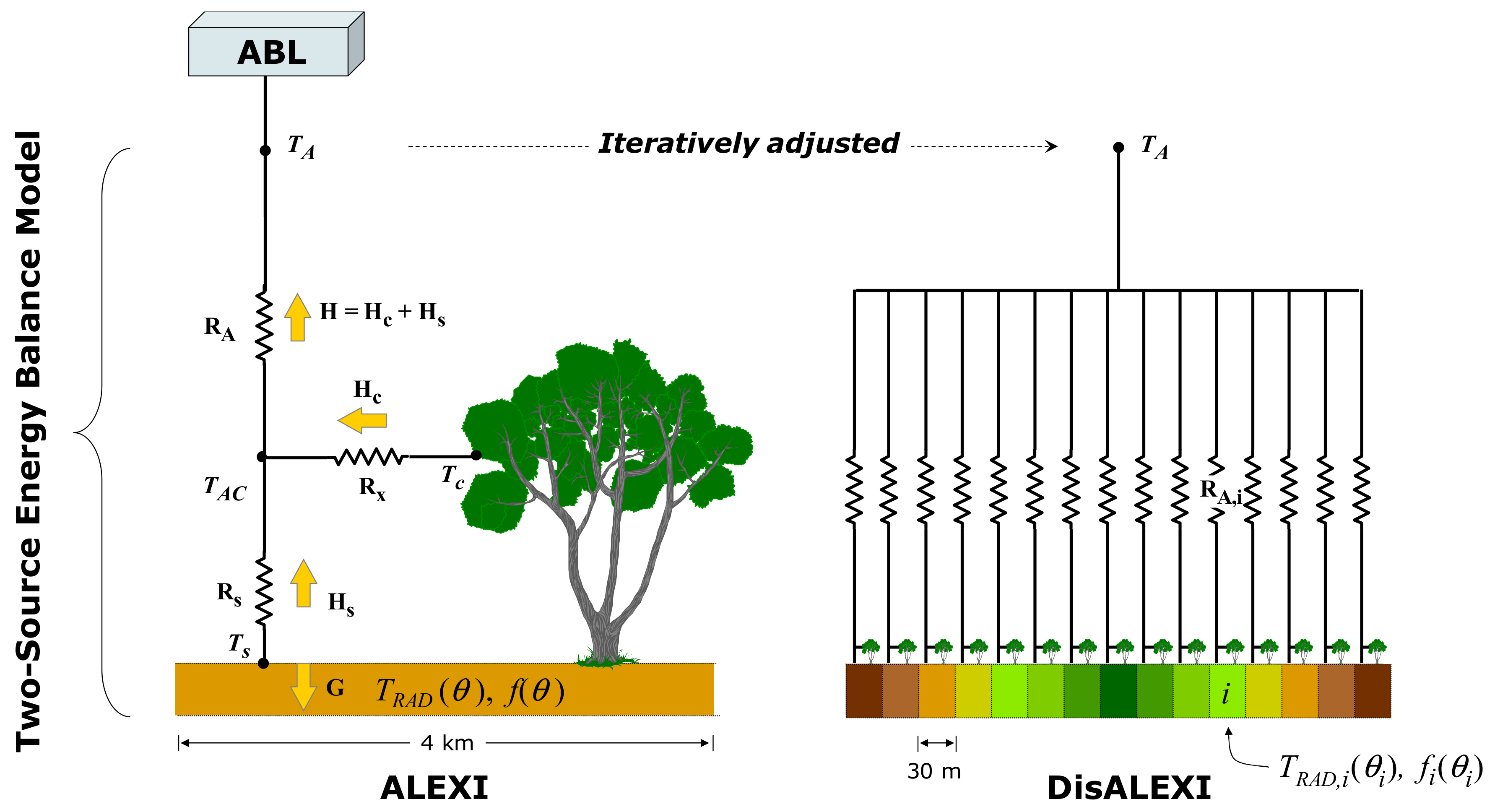
2.2.1. Two-Source Energy Balance Model

Surface energy fluxes were computed over the study domain using the Atmosphere-Land Exchange Inverse (ALEXI) surface energy balance model and associated flux disaggregation technique, DisALEXI. Land-surface exchanges in ALEXI/DisALEXI are governed by the Two-Source Energy Balance (TSEB) parameterization described originally by Norman et al. [23] with improvements in Kustas et al. [24,25]. In the TSEB, the soil and canopy energy budgets (designated with subscripts ‘s’ and ‘c’, respectively) are solved separately:

$$\begin{gathered} R{N}_C=H_C+\lambda E_C \\ R{N}_S=H_S+\lambda E_S+G \\ RN=H+\lambda E+G \end{gathered}$$

(1)

where RN is net radiation, H is sensible heat, λE is latent heat, and G is the flux of heat into the substrate. Sensible heat flux from the vegetation canopy (H_C) and substrate (H_S—typically soil) combine in series to form the net flux H as constrained by component temperature estimates T_C and T_S and the above-canopy air temperature T_A (see Figure 2). The component temperatures are extracted via the system of model equations from radiances inferred by the bulk directional surface radiometric temperature:

$$T_{RAD}{\left(\theta \right)}^4= f\left(\theta \right)T_C{}^4+\left[1-f\left(\theta \right)\right]T_S{}^4$$

(2)

where f(θ) and T_RAD(θ) are at the vegetation cover and directional radiometric temperature at the view angle of the thermal sensor, θ. The model partitioning of net radiation between the canopy and soil components accounts for sun angle, canopy height, leaf area index, and vegetation clumping. The resistance factors describing the coupling between the soil, canopy and atmosphere used in this experiment are described in Norman et al. [23] and Kustas et al. [24,25]. In the TSEB solution, soil and canopy RN are computed via a two-stream canopy radiation model [26], H is constrained by the temperature-resistance network in Figure 2 and G is estimated as described below. The TSEB version used here estimates transpiration, λE_C, with a modified Priestley and Taylor [27] model, with coefficient down-regulation in case of canopy stress as indicated by elevated T_C [28,29]. Soil evaporation, λE_S, is then computed as a residual to Equation (1).

In the original version of the TSEB, the soil heat flux (G) was approximated as a fixed fraction of the net radiation at the soil surface [23]. More recently, the fraction has been computed as diurnal function following Santanello and Friedl [30]:

$$G=c_{g}cos\left(\frac{2\pi \left[t_{g0}+\mathrm{10,800}\right]}{t_g}\right)R{N}_S$$

(3)

where t_g0 is the time (in seconds) from local noon. For a soil substrate, the parameters c_g and t_g are scaling factors that vary with soil moisture. In DisALEXI, the soil wetness regime is represented by a weighted function of the soil evaporative fraction, EF_S:

$$c_g=w{c}_{gmax}+\left(1-w\right)c_{gmin}$$

$$t_g=w{t}_{gmax}+\left(1-w\right)t_{gmin}$$

where

$$w=\frac{1}{\left(1+{\left[\frac{E{F}_S}{0.5}\right]}^8\right)}$$

$$E{F}_S=\lambda E_S/\left(R{N}_S-G\right).$$

For a soil substrate, t_gmax = 100,000, t_gmin = 74,000, c_gmax = 0.35, and c_gmin = 0.31. For a water substrate, as in a wetland, heat storage can be a larger fraction of net radiation [31,32], as further discussed in Section 2.4.2.

2.2.2. ALEXI/DisALEXI

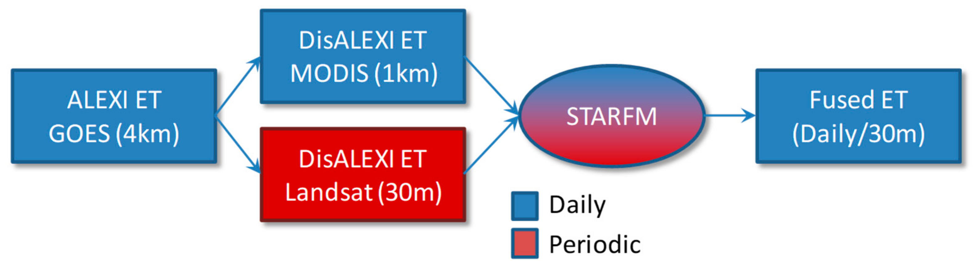
Spatially distributed implementation of TSEB over a landscape requires careful consideration, particularly in the prescription of the air temperature boundary conditions. Using standard meteorological data analyses to define T_A in Figure 2 can be problematic, because small vertical temperature gradient errors with respect to remotely sensed LST data translate into large errors in H and λE [33]. To reduce sensitivity to absolute temperature errors, the regional ALEXI modeling framework employs the TSEB in a time-differential mode [34]. ALEXI estimates the time-integrated sensible heat influx into the atmospheric boundary layer (ABL) during the morning period of ABL development between TSEB executions, typically occurring at an hour after sunrise and an hour before local noon. In this framework, the air temperature T_A (defined at a nominal blending height) is computed internally rather than prescribed, and responds to both the local surface fluxes and the capacity of the ABL to absorb heat. Model surface temperature inputs at these two times are typically acquired via geostationary satellite. The model is sensitive to the morning change in T_RAD, but minimally sensitive to time-invariant absolute errors in T_RAD retrieval [34]. For more details on the ALEXI model, see [34,35].

Daily (24-h) integrated latent heat flux is computed by scaling λE derived at the second T_RAD observation time (pre-noon) by the local solar radiation curve following recommendations by Cammalleri et al. [36]. The daily ET (ETd; mm day⁻¹) can be obtained from the daily latent heat flux (λEd; MJ m⁻² day⁻¹) using the latent heat of vaporization (λ, approximately 2.45 MJ m⁻² to evaporate 1 mm of water at 20 °C)

The spatial resolution of ALEXI flux estimates is constrained by the resolution of the high temporal frequency LST observation source (here, geostationary satellites)—generally on the order of several km. For generating higher resolution ET maps capable of resolving individual crop fields or management units, an ALEXI flux disaggregation approach (DisALEXI) was developed [37,38]. In the DisALEXI step, the TSEB is executed over a gridded model domain using higher resolution LST retrievals from Landsat (30 m, spatially sharpened as described in Section 2.3.1) or MODIS (1 km native or 500 m sharpened) with an initial T_A boundary derived by ALEXI. In current use, this nominal boundary condition is then iteratively adjusted at the ALEXI pixel scale until the DisALEXI ETd field reaggregates to the ALEXI baseline [39]. At the final step in the iteration, the modified T_A field is spatially smoothed to remove boxy artifacts in the output flux maps.

2.2.3. Data Fusion

With disaggregation, periodic Landsat ET retrievals at 30-m resolution can be created—potentially every 8–16 days under completely clear conditions, depending on number of satellites available contemporaneously and position of the study area within the orbital path sidelap. Depending on local cloud climatology, the actual retrieval frequency can be much lower. Anderson et al. [18] suggest that a minimum of one clear-sky retrieval per month is required to recover the seasonal ET curve with reasonable accuracy, but even this frequency can miss important changes in surface moisture and vegetation conditions that occur at weekly or shorter timescales.

To improve temporal representation of ET changes between clear Landsat overpasses, we have employed a data fusion approach that additionally incorporates a second ET datastream, developed at daily timesteps and 1-km spatial resolution using MODIS LST retrievals (Figure 3). The Spatial and Temporal Adaptive Reflectance Fusion Model (STARFM; [40]) was used to fuse the two input datastreams into a single ETd “datacube”, with daily timesteps and 30-m spatial resolution. In brief, STARFM compares MODIS and Landsat image pairs on days when both are available, computes spatial weighting statistics, then applies these weights to downscale MODIS images between clear-sky Landsat overpasses. STARFM was originally developed to fuse surface reflectance imagery, but has also been applied successfully to ET datasets developed over a variety of agricultural and forested landscapes in the United States [20,41,42,43,44,45] and in Spain [46].

2.3. Data

2.3.1. Model Inputs

Model inputs to the ET data fusion system are described in detail in [42]. ALEXI ETd at 4-km spatial resolution, generated over the continental United States (CONUS) from thermal imagery from the combined East and West Geostationary Operational Environmental Satellite (GOES) Imager instruments, serve as the continental-scale baseline for spatial disaggregation. Data from both Landsats 7 and 8 were used to run DisALEXI on overpass days with predominantly clear-sky conditions. Thermal imagery from both instruments was sharpened from native resolution (60–100 m) to the 30-m resolution of the shortwave reflectance bands using a Data Mining Sharpener toolkit [47]. MODIS swath LST products from the Terra platform (MOD11_L2) were projected onto a 0.01° grid containing the Landsat domain and used to run DisALEXI at moderate resolution. Fractional vegetation cover (f) in Equation (2) was computed from LAI products using Beer’s Law, with MODIS LAI obtained from the MCD15A3 product and downscaled to Landsat 30-m resolution using a regression tree approach described by Gao et al. [48]. Surface roughness parameters used in the computation of aerodynamic resistances are tied to landcover type and f as outlined by Anderson et al. [35].

Meteorological inputs of air temperature, solar radiation, vapor pressure, atmospheric pressure, and wind speed were obtained from the Climate Forecast System Reanalysis (CFSR) at 0.25° resolution [49]. These data were used to force both ALEXI and DisALEXI ETd retrievals.

2.3.2. Land-Use Information

Land-use classifications for the 2015 and 2016 growing seasons were generated for the ET intercomparison study over the CA Delta region by Land IQ, Inc., Sacramento, CA, USA (see description in [14]). The classifications included 30 classes in 2015, with 6 new classes added for 2016. These classifications were gridded onto the Landsat modeling domain grid at 30-m resolution and were used to quantify changes in land use between years.

2.3.3. Flux Datasets

Micrometeorological data from eight eddy covariance (EC) systems operating within the domain were used to evaluate the fused WY 2015–2016 ET timeseries over different landcover types (

Table 1. Flux towers used in the analysis.

Site	Tower	Name	Cover	Latitude	Longitude
Borden Ranch	Lodi1		vineyard	38.2894	−121.1178
Borden Ranch	Lodi2		vineyard	38.2805	−121.1176
Twitchell Island	US-Tw1	West Pond	old wetland	38.1073	−121.6468
Twitchell Island	US-Tw4	East End	young wetland	38.1028	−121.6413
Twitchell Island	US-Twt		rice	38.1087	−121.6530
Twitchell Island	US-Tw3		alfalfa	38.1151	−121.6468
Sherman Island	US-Myb	Mayberry	intermediate wetland	38.0498	−121.7650
Sherman Island	US-Sne	Sherman	new wetland	38.0369	−121.7547

).

Two flux towers were operating in the Borden Ranch viticultural area north of Lodi, CA in adjacent vineyards with Pinot noir vines of age ~12 years (Lodi1) and 9 years (Lodi2) during the experiment timeframe. Row direction is East–West in each vineyard. Eddy covariance systems deployed in both fields have collected measurements of surface energy and carbon fluxes since 2013, with details provided by Kustas, et al. [21].

Also operating during the study period were four AmeriFlux EC towers installed on Twitchell Island, at the core of the Delta region. These towers include two sites in water-intensive crops: rice (US-Twt; doi:10.17190/AMF/1246140) and alfalfa (US-Tw3; doi:10.17190/AMF/1246149). Two additional towers are sited in restored wetlands: the East End wetland (US-Tw4; doi:10.17190/AMF/1246151), restored in 2014, is largely vegetated with some open water channels, while the West Pond site (US-Tw1; doi:10.17190/AMF/1246147) dates back to 1997 and the vegetation is now fully closed. Two AmeriFlux tower sites on nearby Sherman Island were also used, sampling the mature Mayberry wetland (US-Myb; doi:10.17190/AMF/1246139) established in 2010 and the sparsely vegetated US-Sne wetland (doi:10.17190/AMF/1418684), converted from pasture and newly flooded in December of 2016. Together, the sites Sne, Tw4, Myb and Tw1 represent a chronosequence in the development of restored wetlands, from newly established to stable and fully vegetated. Details regarding the Twitchell and Sherman Island measurements are provided by Eichelmann [22].

The EC technique is known to produce turbulent flux estimates that do not fully close the observed energy budget, yielding closure errors 1 − (H + λE)/(RN − G) typically on the order of 10–20% or higher in some cases [50,51]. While not fully understood, possible explanations for the lack of closure include instrumental bias, incomplete characterization of the substrate heat flux, G, and possible mismatch in sampling footprint between the turbulent flux and available energy measurements. For example, flow distortions associated with non-orthogonal sonic anemometer configurations (such as used at all towers in Table 1) are suspected to result in 10% underestimation of λE [52,53,54,55]. For comparison with model estimates which assume closure, observed latent heat fluxes over non-wetland surfaces have been closed by assigning the residual of the energy balance to λE. For the wetland sites, closure has not been attempted due to uncertainties in measuring heat storage, G, within the water substrate given the dynamic bathymetry and fluctuating water tables. For those sites, observed λE was increased by a nominal 10% to account for flow distortion effects.

2.4. Model Modifications

2.4.1. Cold Season Bias

Prior evaluations of DisALEXI datacubes over the California vineyard sites in comparison with tower data identified a small wet bias in the cold season fluxes [42]. This bias has been tied to the ALEXI baseline conditions, which tend to overpredict ET during the short morning rise window period characteristic of the late fall to early spring. A global correction approach is under development for the operational ALEXI modeling framework.

In the short-term, to accommodate this existing bias and to improve accuracy of seasonal water use estimates, a generalized second order empirical correction was derived as a function of day of year (DOY) from model comparisons with 2015–2016 fluxes from the Twitchell Island flux sites US-Tw1 (latter half of year), US-Twt, and US-Tw4 (US-Tw3 was excluded due to noise related to frequent alfalfa cutting) and confirmed against all sites. The function is symmetric with DOY in this region, yielding minimal correction mid-season and a 50% reduction of fluxes near the beginning and ending of the year. Note that cold-season evaporative fluxes are small to begin with, so the correction has only minor impact on seasonal modeled ET. This correction was applied uniformly across the domain for both the 2015 and 2016 WYs. At all flux sites, model-measurement agreement improved with this correction (see Section 3.1).

2.4.2. Wetland Energy Balance

In wetlands, the substrate heat storage term, G, is known to be significantly larger than for a soil layer due to the large heat capacity of water. If this is not accounted for, instantaneous λE retrieved via energy balance at the time of midday satellite overpass will be overestimated, leading to biased upscaled daily ET estimates.

For soil, the c_g parameter in Equation (3) is set to values varying from 0.3 to 0.35 as described in Section 2.2.1. In this study, following Burba and Verma [31] we use a higher value of c_gmax = c_gmin = 0.6 for pixels in the model domain classified as “wet herbaceous/sub-irrigated pasture” in the LandIQ datasets. Visual inspection confirmed that this class was best associated with known wetlands within the central Delta region.

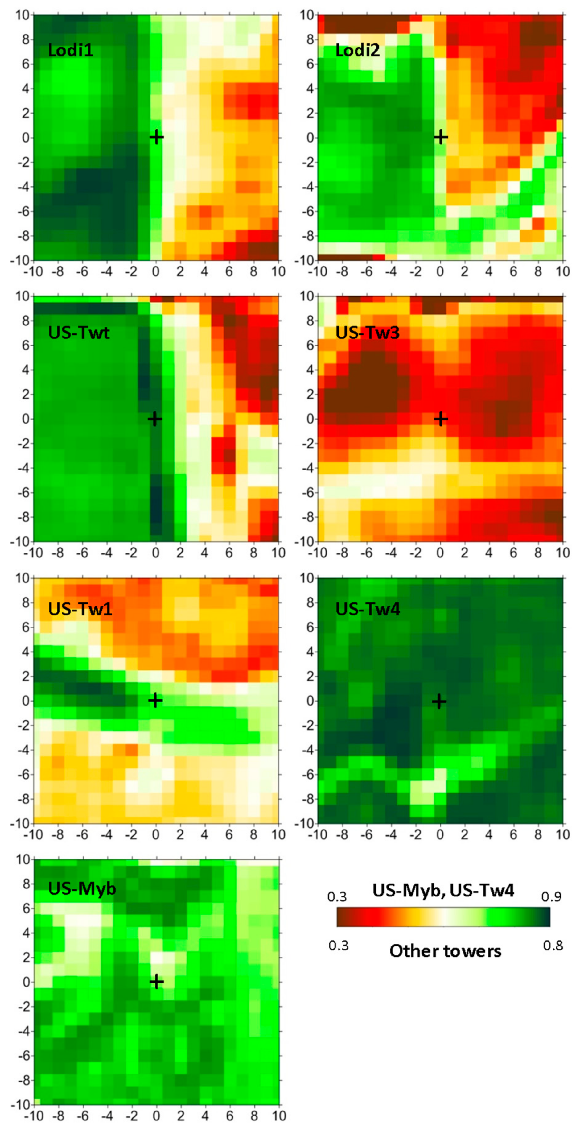
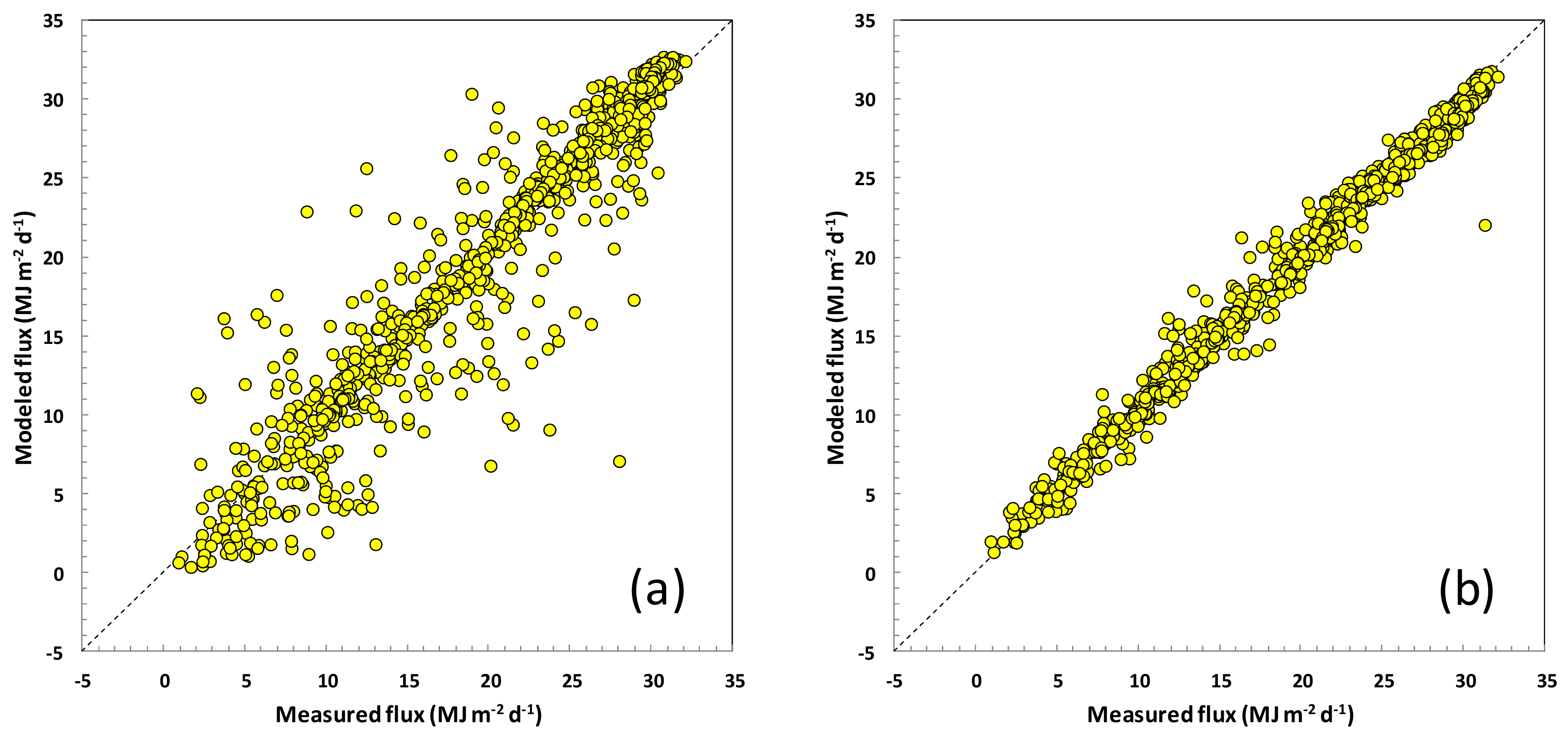
2.5. Model—Measurement Comparisons and Tower Representativity

To conduct timeseries comparisons between measurements and daily model estimates, model data were extracted and averaged over a 3 × 3 pixel (90 × 90 m) window near each tower site, offset in the direction of mean incoming wind to approximate seasonal daytime fetch contributing the majority of the daily flux. Over more heterogeneous sites, for example for towers located at a field edge, care is required to select representative pixels for comparison with observed fluxes.

To support the model extraction, we assessed the spatial representativity of tower observations with respect to the surrounding landscape, using the model fluxes as a proxy for the true flux distribution around each tower site. A 3 × 3 window was shifted ±10 pixels around the pixel containing the tower, a two-year time series of model fluxes was extracted at each window location, and statistical metrics of model-tower observation agreement were computed, including the Nash and Sutcliffe [56] coefficient of efficiency, NSE (note that US-Sne was not included in these analyses due to short record length). Maps of NSE were used to select small window offsets (a few pixels) for evaluating model performance. These offsets were not selected to maximize NSE, but simply to avoid field boundaries and edge effects and to restrict model extractions to lie within the representative vegetation class. Assuming the relative spatial variability in surface fluxes is reasonably represented by the model, these maps can also provide qualitative information about local surface features that may affect turbulent flux observations, and the extent to which the tower data are representative of field-scale water use.

3. Results

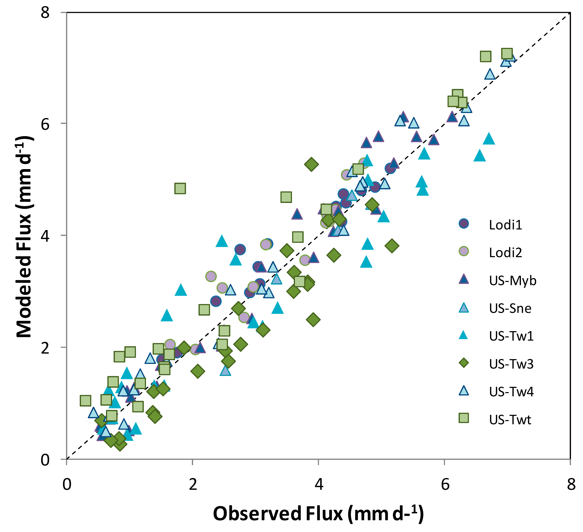
3.1. Model Evaluation at Flux Tower Sites

Table 2. Statistical metrics of model performance for estimating ET (mm day⁻¹) at daily, weekly, monthly, and yearly timesteps. Daily metrics generated without the cold-season model bias correction are also provided (W/O corr).

Timescale	Tower	N	<O>	MBE	RMSE	NSE	R2	MAE	RE
DAILY	Lodi1	450	3.44	0.11	0.8	0.761	0.766	0.634	0.184
	Lodi2	438	3.35	0.10	0.67	0.747	0.767	0.523	0.156
	US-Myb	818	3.11	0.10	0.81	0.836	0.851	0.631	0.203
	US-Sne	161	3.70	−0.31	0.84	0.530	0.738	0.703	0.190
	US-Tw1	818	3.03	−0.11	0.99	0.788	0.792	0.802	0.265
	US-Tw3	817	2.77	−0.39	1.09	0.558	0.641	0.808	0.291
	US-Tw4	818	3.57	0.16	0.77	0.895	0.900	0.603	0.169
	US-Twt	817	2.96	0.48	1.24	0.738	0.795	0.906	0.306
	ALL	5241	3.10	0.08	0.95	0.778	0.791	0.723	0.233
W/O corr	ALL	5241	3.10	0.24	1.01	0.705	0.766	0.788	0.254
WEEKLY	ALL	720	3.18	0.09	0.76	0.842	0.851	0.571	0.179
MONTHLY	ALL	169	3.19	0.08	0.58	0.898	0.905	0.436	0.137
YEARLY	ALL	10	3.02	0.07	0.28	0.018	0.636	0.235	0.078

provides statistical metrics comparing fused ET timeseries, extracted as described in Section 2.5, and fluxes observed at all eight flux sites as well as for all sites combined. The average root-mean-square error (RMSE) is ~0.95 mm day⁻¹, with a mean bias error (MBE) of 0.08 mm day⁻¹ and a relative error (RE = MAE/<O>) of 23% at the daily timescale, where MAE is the mean absolute error and <O> is the mean observed flux. Relative errors reduce to 18%, 14%, and 8% at weekly, monthly, and yearly timescales, respectively, due to time averaging of random errors. This performance is close to the target of 0.8 mm day⁻¹ error suggested by Seguin [57] for actionable ET information in agroecology. The data fusion approach also supports the high temporal (near daily) and spatial (sub 100-m) requirements specified in that study. Maps of NSE from the tower representativity analyses described in Section 2.5 are shown for each site in Figure 4, with green indicating areas where model flux timeseries are in best agreement with the tower fluxes.

Without the cold season correction, the RMSE, MBE, and RE at daily timescales increase to 1.01 mm day⁻¹, 0.24 mm day⁻¹, and 25%, respectively (Table 2), indicating the correction has a small but positive impact on the collective statistical agreement with tower fluxes used in this study. The wetland storage term correction also had a positive impact on model performance at the established wetland sites (US-Myb, US-Tw1, and US-Tw4). Collectively for these three sites, ET RMSE is reduced from 1.34 to 0.87 mm day⁻¹ and MBE by 0.87 to 0.05 mm day⁻¹ by adopting the larger G coefficient for wetland classes.

Model performance at individual sites is discussed in greater detail below.

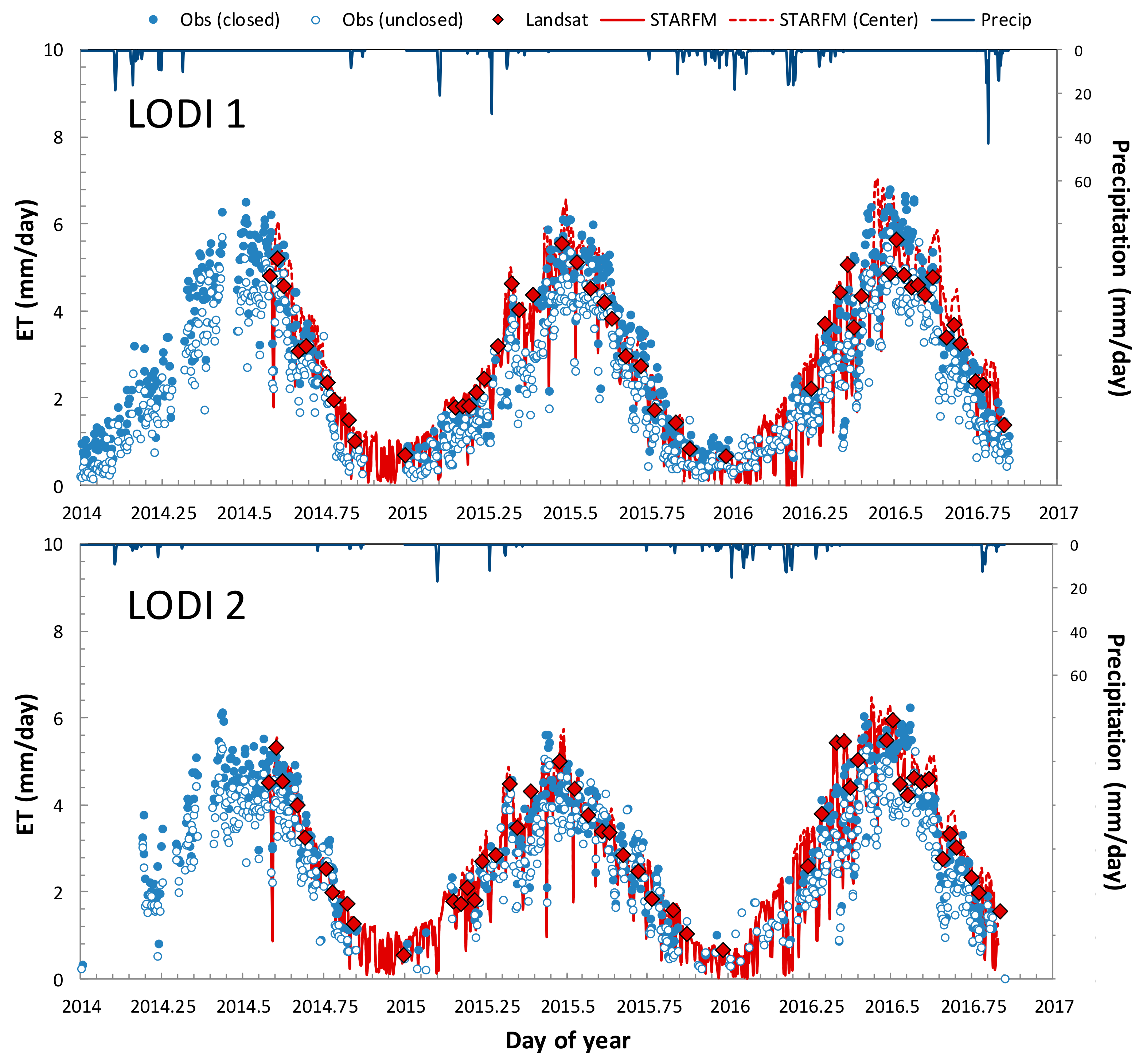
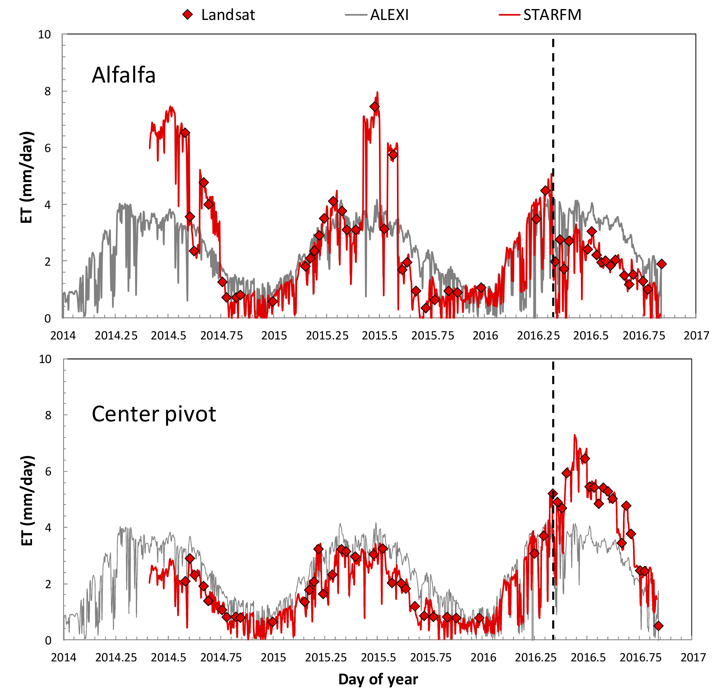
3.1.1. Lodi Vineyard Sites

With the cold-season correction, modeled ET agrees well with observations at both vineyard sites in 2015–2016 (Figure 5). Model estimates extracted close to the tower underestimate closed ET fluxes on some days during the peak growing season in 2016 at the northern vineyard site 1. These have been identified these as being days with highly advective conditions and large residual EC closure errors, leading to both enhanced modeling and measurement uncertainties at this site. These peak fluxes are better captured by model fluxes extracted near the north central part of the field (also indicated in Figure 5)—a region of more vigorous vine growth and yield production [42]. Based on the tower representativity analyses in Figure 4, this region shows lower values of NSE relative to surrounding areas when computed from the full two-year timeseries, but higher values of NSE when analysis is isolated to the peak growing season. Smaller differences in NSE are observed between the field edge and center in the southern vineyard, indicating more homogeneous conditions. Despite these effects, RMSE for model fluxes near the towers was low over these two water years, with values of 0.80 and 0.67 mm day⁻¹ at sites 1 and 2, respectively.

Maps of cumulative ET for the 2015 and 2016 growing seasons (nominally April–October; DOY 100–300) are shown in Figure 6, along with the change in seasonal ET between these years. The site 1 vineyard displays similar ET in both years, while seasonal ET in the southern vineyard increased by approximately 150 mm in 2016 in response to a 50% increase in irrigation. The ET difference map highlights other fields in the vicinity that underwent significant changes in water management and cultivation between years. For example, irrigation in the alfalfa field to the south of Lodi2 appears to have been curtailed in early May of 2016 (Figure 6 and Figure 7), perhaps in response to water allocation restrictions. At about the same time a center pivot was activated in a field about 3-km south of Lodi2 (Figure 6 and Figure 7). These changes in land management are both signified by a distinct departure in local water use from the 4-km ALEXI average ET (Figure 7). Three additional fields were not irrigated to the same extent as in 2015 (light patches in the Figure 6 difference map), while other fields consumed more water in 2016 (dark green patches in the difference map). In balance, the overall change in total annual ET over this region between water years was small.

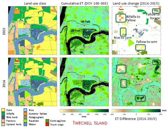
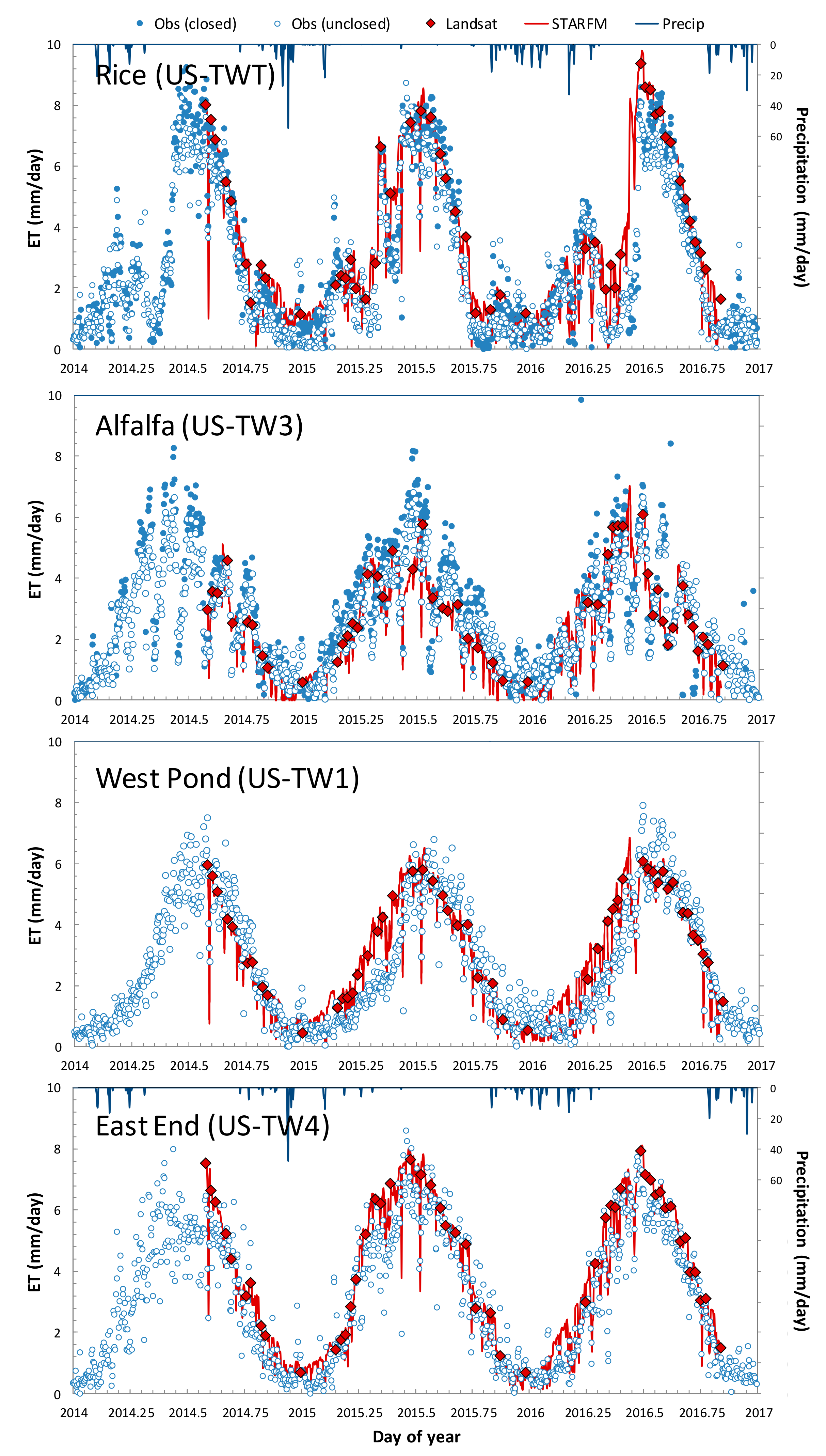
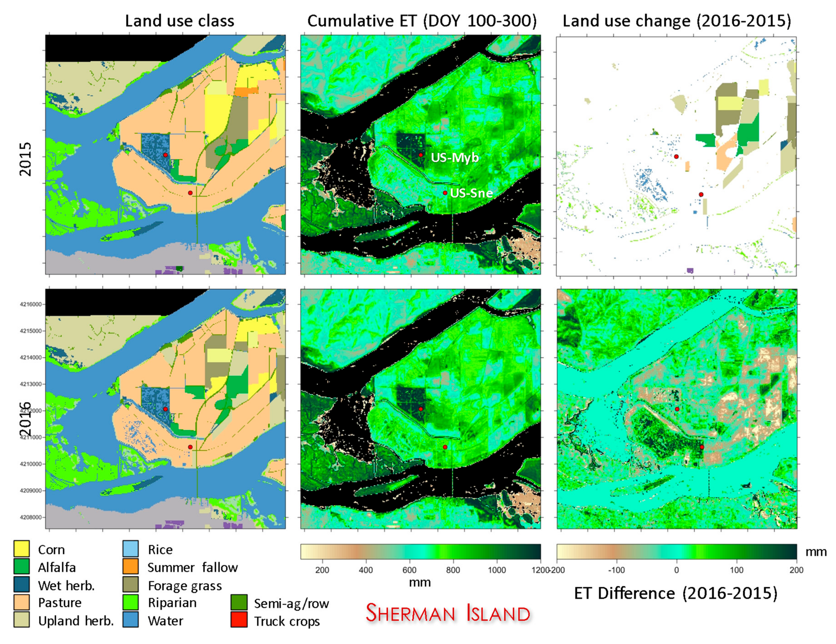
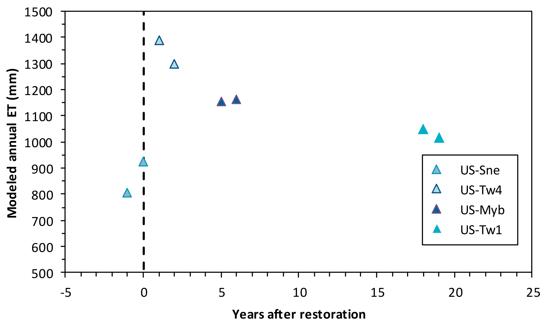
3.1.2. Twitchell Island Sites

Flux comparisons for the Twitchell Island towers are shown in Figure 8, with cumulative and difference ET maps in Figure 9. The fused ET performed reasonably at the rice site (US-Twt), with RMSE/MBE of 0.95/0.08 mm day⁻¹. The observations reflect the distinctive water-use phenology for rice cultivated in this region. Rice paddies are flooded over winter for bird habitat, and then drained in springtime to prepare the fields for planting, together yielding an early season peak in ET. This is followed by a steep increase in ET as the fields are reflooded after the seedlings have reached a threshold height. These seasonal water use characteristics are generally reconstructed by the remote sensing timeseries, although the modeled spring decreases associated with paddy draining are not as deep as observed in 2016. In addition, some short-term transient responses to rainfall (e.g., in the winter of 2014–2015) are not captured by the fusion process.

Phenology in alfalfa is particularly difficult to capture with remote sensing at Landsat scale due to frequent (approximately monthly) cutting and regrowth cycles (US-Tw3). The probability of catching peak and minimum flux states is greatly improved by incorporating data from two Landsat platforms, with a combined overpass frequency of 8 days. While most of the cuttings are reflected in the fused ET timeseries, sometimes peak ET values between cuttings are missed, for example around DOY 220 (0.6 fractional year) in 2015 and 2016. This contributes to an underestimation of seasonal water use by about 15% over this 2-year period. Close examination suggests this is due in part to a footprint issue. The NSE map for this field (Figure 4) indicates an area of low tower-model agreement around the tower and to the west and northwest, where model fluxes are 0.9 mm day⁻¹ lower than observations on average. The alfalfa crop in this field is an older planting and late in the summer the canopy in this part of the field does not fill in well, with declining photosynthetic capacity indicated by a decrease in tower carbon flux and greenness measurements relative to periods of comparable radiation load in the spring. The Landsat TIR imagery for these late-summer retrievals, even prior to sharpening, show higher surface temperatures in this part of the field—further indicating lower local evaporative rates relative to surrounding pixels classified as alfalfa. In future work, rigorous footprint analyses will be employed to ascertain off-field and advective contributions to tower latent heat fluxes during these periods.

Comparisons with observations from wetland tower sites on Twitchell Island indicate that the wetland storage correction has the effect of lowering peak seasonal evaporative flux by approximately 30%. The local heterogeneity in ET around these towers is large relative to the other sites due to small-scale structure in and around the reconstructed wetlands, particularly surrounding the older West Pond site (US-Tw1). Model fluxes in pixels within the West Pond boundaries agree well with observations at US-Tw1 (the narrow green band of high NSE in Figure 4), while ET in younger wetland areas surrounding West Pond is 0.5–1.0 mm day⁻¹ lower (red regions in Figure 4). Conditions are more uniform at the East End site (US-Tw4), except along the grass berms separating wetland plots where model fluxes are 0.9 mm day⁻¹ lower than at the tower site. Seasonal model ET fluxes trace the observed phenological cycles at both sites, although the delay in spring ramp-up at West Pond, caused by a dense mat of litter delaying new photosynthetic growth, is not cleanly captured (Figure 8). This discrepancy may be due in part to mixed pixel contributions in the modeled fluxes from younger neighboring wetlands.

Twitchell Island lies within the CA Delta region covered by the Land IQ landcover datasets for 2015 and 2016; therefore, at this site we can investigate commensurate changes in both water and land use (Figure 9). Many of the largest changes in water use are associated with changes in crop type or land management. For example, decreases in ET are evidenced in areas where land use changed from alfalfa to fallow and from rice to corn. Fallowed fields in 2015 that were converted to crop production in 2016 show large increases in seasonal ET. A patch in the northeast corner of the subset area with >200 mm increase in ET in 2016 was not associated with recorded land-use change (reported as corn in both years), which might indicate either an error in classification or a change in water management strategy.

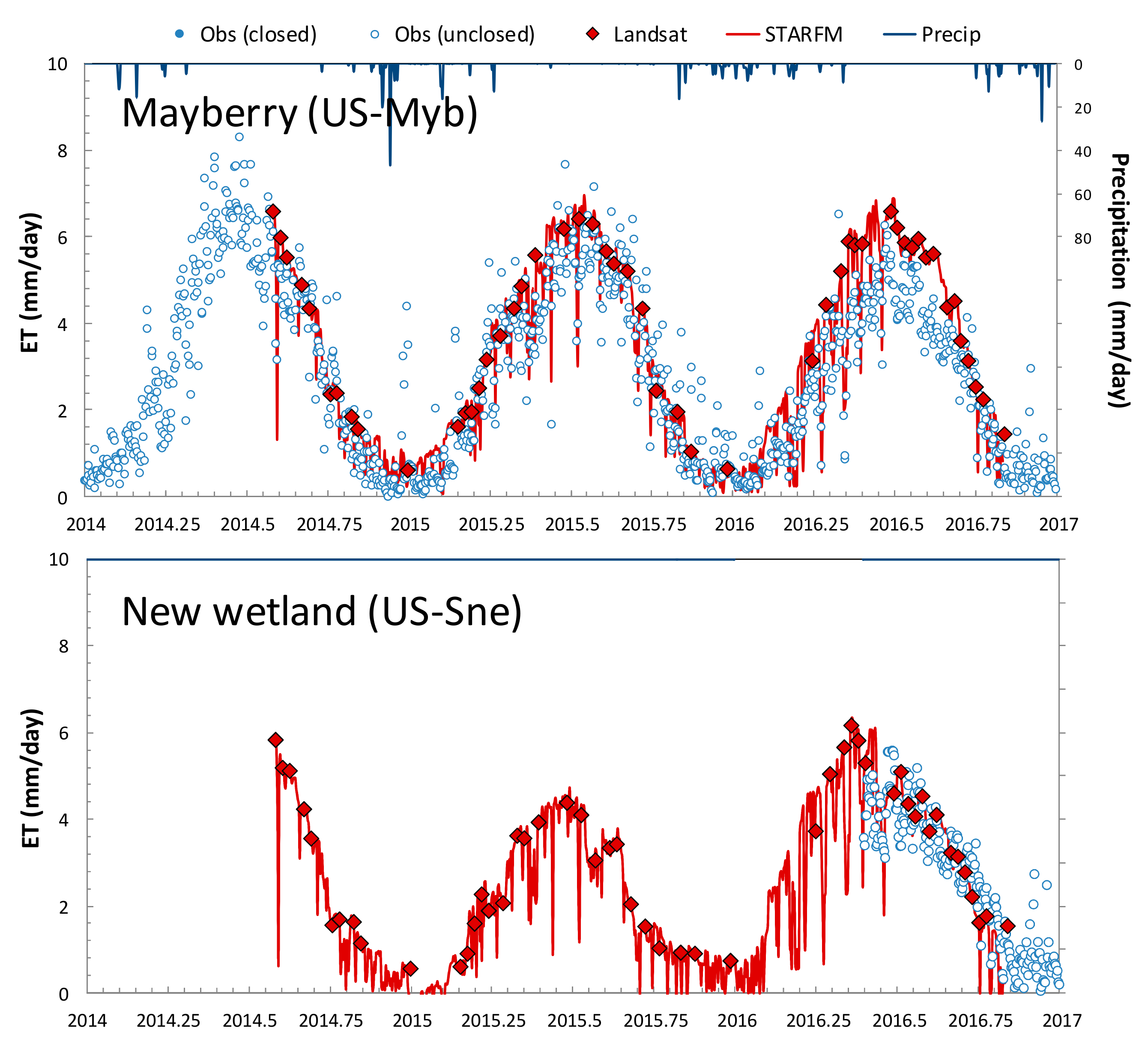
3.1.3. Sherman Island Sites

With the wetland heat storage correction, seasonal patterns in modeled and measured daily ET are in general agreement at the Mayberry wetland site on Sherman Island (Figure 10), with RMSE/MBE of 0.81/0.10 mm day⁻¹ (Table 2). In 2016, saltwater intrusion had a notable effect on vegetation health, resulting in a decrease of both observed carbon and water fluxes relative to 2015. Why this decrease in 2016 was not captured by the remote sensing model is under investigation; the remotely sensed 30-m land-surface temperature and LAI model inputs over this site do not suggest a significant change in ET between years. Enhanced heterogeneity in surface conditions around the site (Figure 4) may be a contributing factor. The Mayberry wetland was designed with wide open-water canals for bird habitat which may be being captured in the remote sensing data, reducing sensitivity of the modeled fluxes to vegetation condition.

Evaporative fluxes at the new Sherman Wetland (US-Sne) tower site are also well represented by the modeling results. This site was a pasture prior to 2016 (consistent with the Land IQ classification, Figure 11), and was periodically inundated due to its low-lying topographic setting. In 2016, the pasture was excavated in preparation for restoration, and for much of that year was covered in disturbed peat and mineral soils as berms were being constructed. Flooding commenced in October, near the end of the fused ET timeseries in Figure 10. Disturbance and flooding, along with higher rates of rainfall during the prior cold season, lead to an increase in annual ET in the US-Sne wetland on the order of ~150 mm in 2016 relative to the severe drought year of 2015.

3.1.4. Multi-Site Monthly ET

Figure 12 summarizes the validation results in a scatter plot of modeled vs. observed monthly average ET for all flux sites combined. In general, monthly RMSE/MBE of 0.58/0.08 mm day⁻¹ provides an indication of the level of confidence we can assume in Delta-wide water use analyses, although some classes such as alfalfa (represented by US-Tw3) and rice (US-Twt) may have larger biases. The sample with the largest discrepancy in Figure 12 represents the rice site (US-Twt) during the spring drainage period in 2016, when the model overestimated observed ET by ~2.5 mm day⁻¹ on average (see also Figure 8).

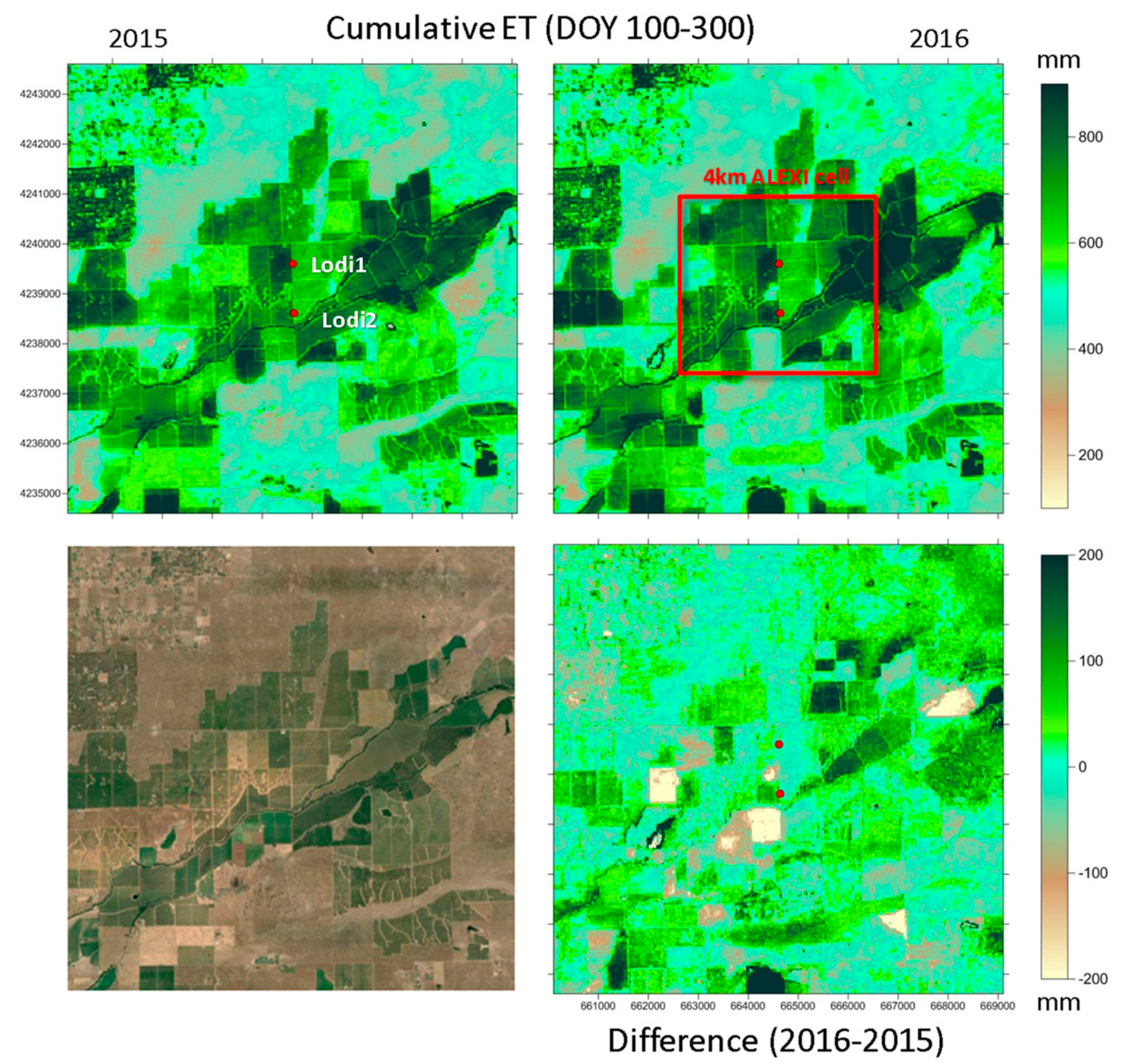
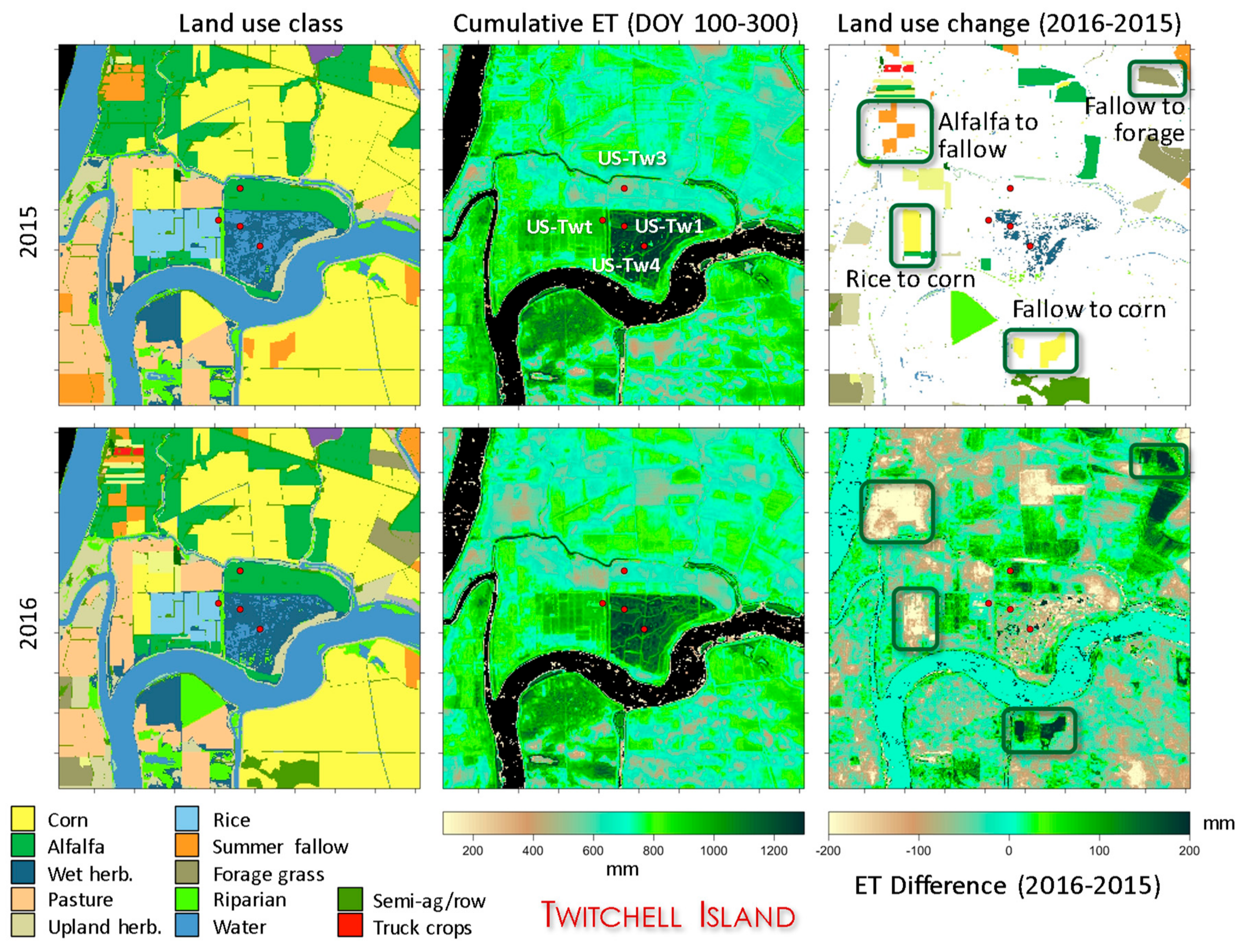
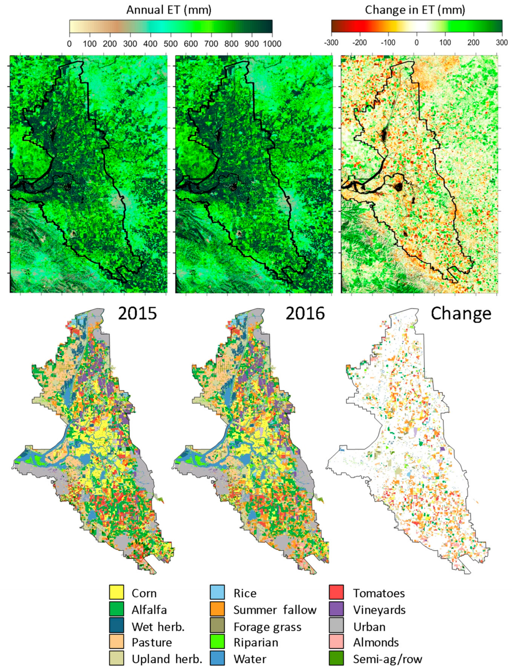
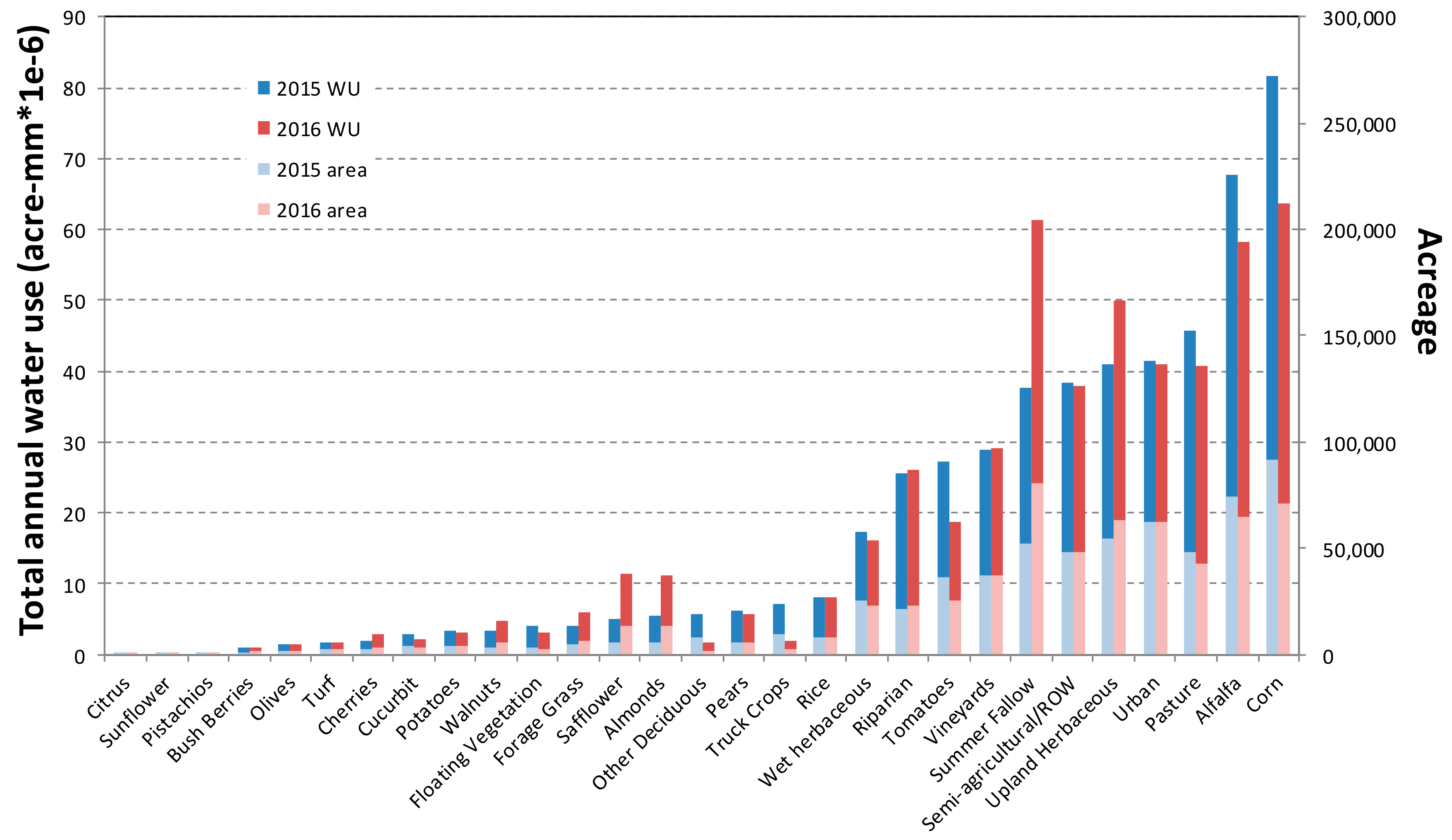
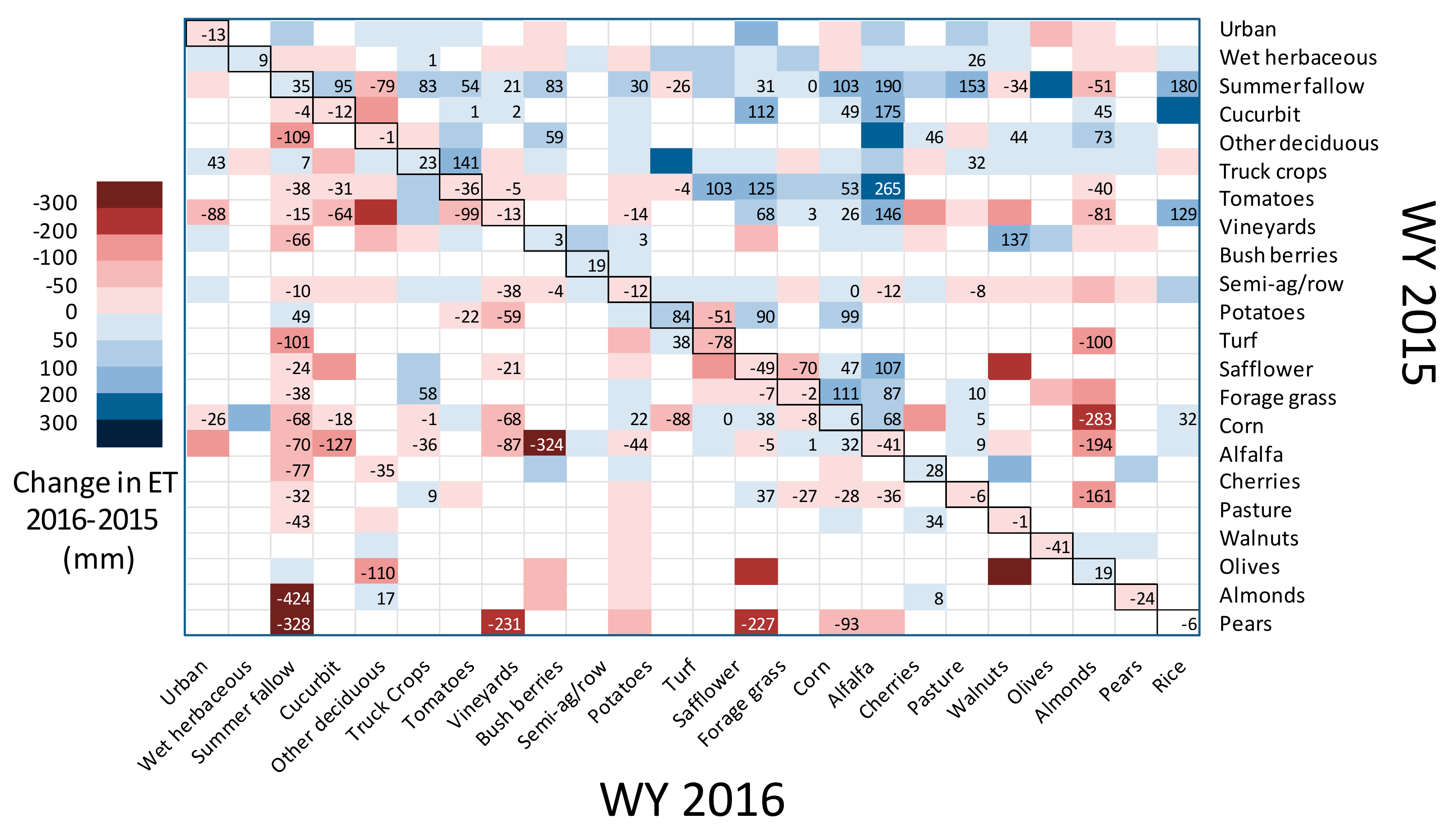
3.2. Regional Changes in Land Use and Water Use

Maps of annual ET over the Landsat modeling domain for WY 15 and 16 are shown in Figure 13, along with the change in ET between water years (2016–2015). Land use and land-use change are mapped in the second row. Averaged over the Delta subregion, annual ET from the fusion results changed by only 3 mm (0.4%), from 822 to 819 mm yr^-1, between years. (Note: estimates for ET from open water bodies within the Delta boundaries are not included in this average.) This translates to a total average consumptive water of 1986 thousand acre feet (TAF) per year across the legal Delta area for the 2015–2016 water years, with a decrease of 7 TAF between years.

Dominant modeled ET changes within the Delta typically occur at field-scale and are distributed relatively uniformly across the domain. In general, areas that were classified with a change in land use between water years also registered the largest changes in ET, with an average value of 102 mm absolute ET change in pixels where there was land-use change, and 71 mm where there was no change recorded. The most extensive land-use change reported was conversion to summer fallow, with a total of 29,000 acres added in 2016, followed by a decrease in corn production area by 21,000 acres and an 11,000 acre decrease in tomato cultivation.

A ranked histogram of average modeled annual ET by land-use class for WY 2015 and 2016 is provided in Figure 14 as determined for areas lying inside the legal Delta boundaries, as well as the area covered by each class in each year. For most classes, the average annual ET is similar between years. The most notable exceptions are almonds, for which the data suggest a reduction of 197 mm year⁻¹, and a similar increase (170 mm year⁻¹) for the “other deciduous” class. Given that water management in almonds is not expected to have changed drastically between years, this suggests confusion or change in classification methodology between these two years. Indeed, the inferred area of almond coverage more than doubles between 2015 and 2016, while area for other deciduous is reduced by 80%. In this case, annual water consumption could be a useful additional factor to consider in the classification methods.

The top classes ranked by annual modeled ET include riparian areas, rice, pears, and almonds. Near the bottom are the urban, pistachio, wet herbaceous, summer fallow, and cucurbit classes—all with annual ET < 750 mm. Vineyards average less than 800 mm year⁻¹, in part reflecting advantages of regulated deficit irrigation for achieving high quality grapes for wine production. The average ET for the wet herbaceous/sub-irrigated pasture class is ~700 mm year⁻¹ is consistent with measurements made at a pasture site on Sherman Island, active from 2007 to April 2015 (US-Snd; see Figure 10 in [17]). However, it is significantly less than the ET of 1180 mm year⁻¹ on average modeled around the three established wetland tower sites (US-Myb, US-Tw1, and US-Tw4). The average observed fluxes at these sites for the 2015–2016 water years, accounting for 10% EC correction due to non-orthogonal flows, is 1150 mm year⁻¹. The lower ET attributed to the wet herbaceous/sub-irrigated pasture class reflects the broad definition of this class, including significant acreage in pastures to the north that are outside the Delta wetland restoration zone.

In future studies, new high-resolution wetland mapping algorithms (e.g., [58]) can be employed to more accurately identify pixels with a water substrate requiring modified treatment within the energy balance model. Water use specifically by restored wetlands is likely to reside near the upper end of the distribution in Figure 14, similar to the floating vegetation and riparian classes. Using the chronosequence of wetland flux sites as an indicator of wetland evolution post-restoration, annual modeled ET shows a decreasing trend with time (Figure 15). This decrease results as open water within the restored unit is increasingly encroached by vegetation which exerts stronger regulation on evaporative losses. This finding could be important when considering the long-term water and carbon tradeoffs associated with restoring drained agricultural peatlands to restored, flooded wetlands. However, other factors like the initial design of the wetland or disturbances from insect infestation can also significantly affect wetland ET and can lead to trajectories that differ from those seen in Figure 15 [22]. More sites will be required to confirm a typical trend in consumptive water use by restored wetlands.

When viewed from the perspective of total water use over the Delta region, weighting by areal coverage for each class, the rankings change significantly (Figure 16). On a total water use basis, corn, alfalfa, and pasture classes rank highest. Total water use dropped between 2015 and 2016 for these high water-use classes due to reduction in planted area, possibly in response to water allocation pressures exerted by the long-term drought. Urban water use is ranked next; however, the accuracy of model estimates in urban settings has not yet been evaluated and will be sensitive to errors in specifications of resistances, surface emissivity, LAI, and parameterization of heat storage. Upland herbaceous and summer fallow classes rank high due to large area coverage, both with large increases in total water use for 2016 due to expanded acreage.

With these combined land-use and ET datasets, changes in water use that accompany specific conversions in land use can be estimated (Figure 17). These estimates reflect water consumption rates that may be specific to the unique climate and management approaches adopted in response to the multi-year drought preceding the period of analysis. They also include both ET model and classification uncertainties. Still, they may provide some guidance regarding expected short-term water-use savings involved in specific land-use conversions in periods of limited water availability. With additional years of data, climate contributions due to interannual variability should be reduced on average.

The model results suggest that the largest water-use savings were realized in fallowing land, which is not unexpected. Particularly large ET reductions were observed for pear and rice conversion to summer fallow. Transition from alfalfa to vineyard also resulted in significant water-use reduction. However, water requirements in these new vineyards will increase in the out-years as the vines mature. Furthermore, conversion to permanent crops like vineyards and orchards effectively “hardens” the water demand in the long term, allowing less flexibility in terms of partial-season irrigation or fallowing in response to drought. Increased water use is most notably associated with conversion of truck crops to alfalfa, as well as cropping of fields that were fallowed in 2015.

The water accounting information in Figure 14, Figure 15, Figure 16 and Figure 17 can be used to assess specific scenarios of water use change in response to incentives (e.g., carbon or conservation credits) and stressors (e.g., restrictions in water allocations in times of drought). For example, if the carbon market became more viable and farmers were incentivized to transition a percentage of fallowed or pasture land to wetlands, the resulting change in regional water demands could be predicted.

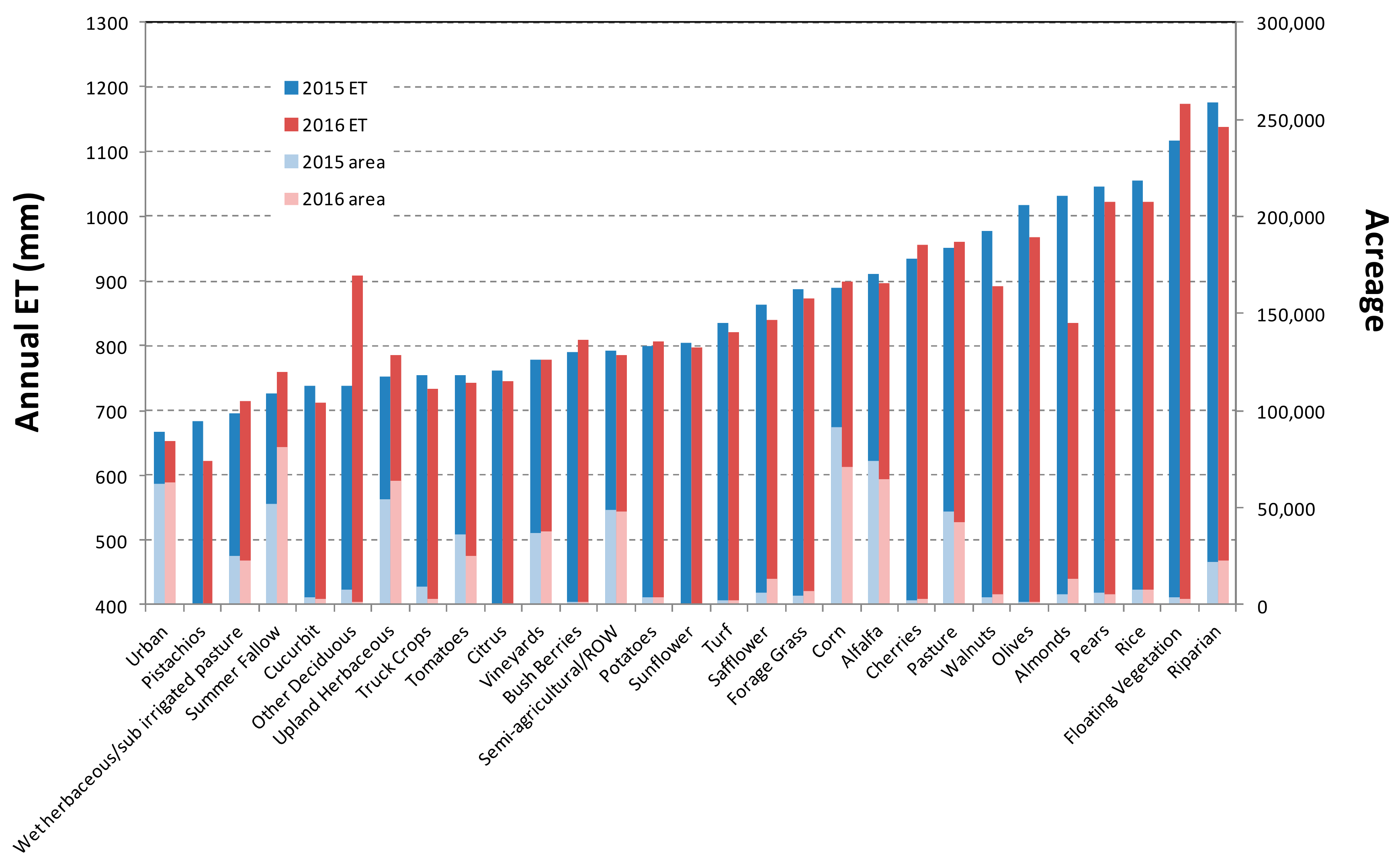
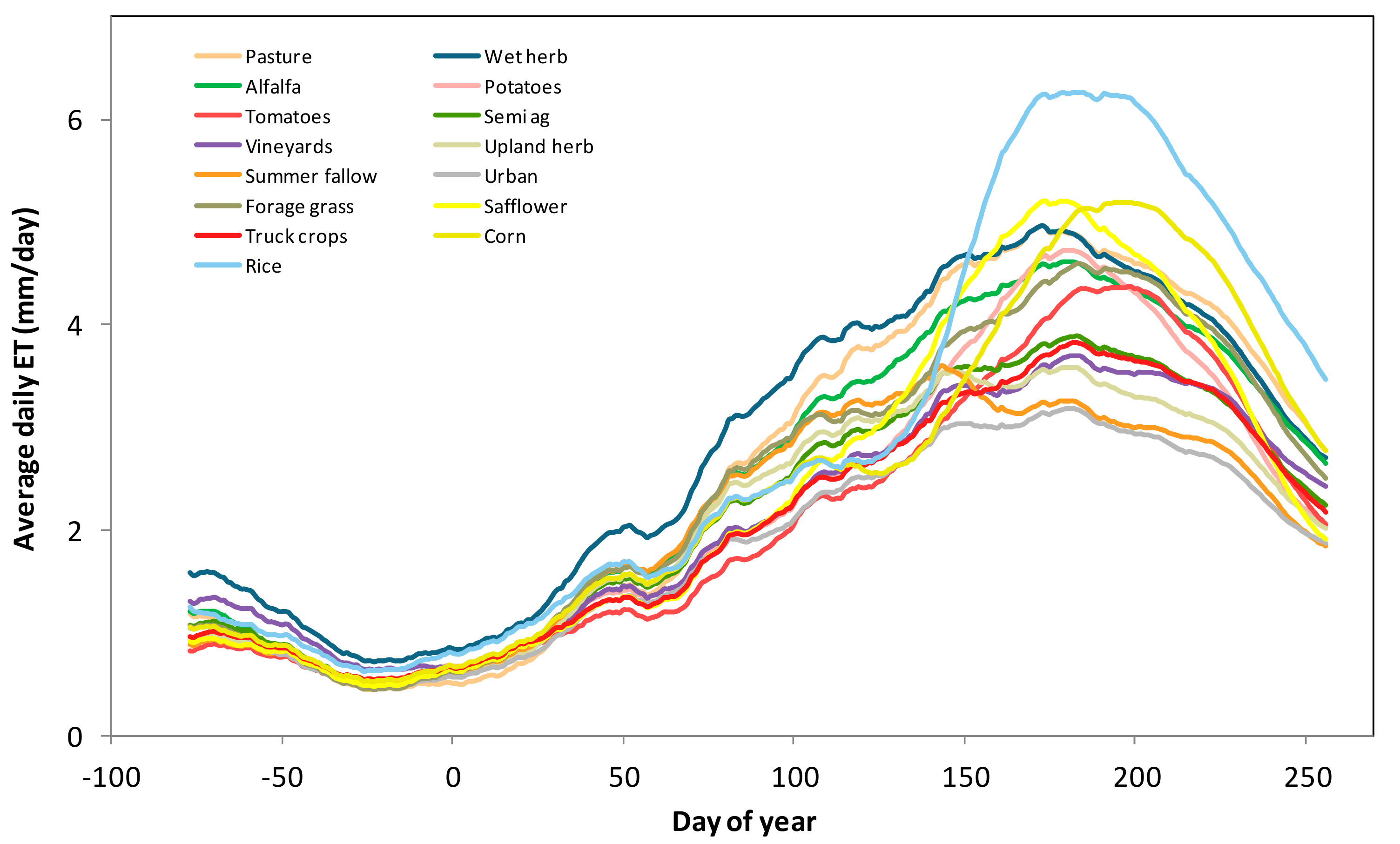
3.3. Characteristic Water Use Curves

Along with differences in total annual consumptive use (Figure 14), the major land-use classes within the Delta region also have distinctive seasonal patterns in daily water use (Figure 18). Cataloging characteristic water use/demand curves by land use can benefit grower decision making in times of limited water availability, as well as management of water delivery systems active within the Delta region. The temporal ET patterns shown in Figure 17 reflect both crop phenology and management activities. Water use by corn, rice and tomatoes, for example, peaks later in the season in comparison with other landcover classes, while wet herbaceous and urban class water use is more uniformly distributed throughout the main growing season.

The seasonal water use curve for a given crop will also depend on in-field water management strategy, which may become more diverse over landscapes in times of water use restrictions. For example, one strategy for irrigating alfalfa under limited water supply is to use the full allocation in the early season to obtain maximal biomass in the early cuttings then to turn off irrigation for the remainder of the season. The benefits of such a strategy are that these early cuttings typically have the highest yields of the season, stand health is not greatly compromised in future years as it might be in deficit irrigation or fallowing, and the allocation is fully utilized before additional restrictions may be levied later in the season [59]. This strategy may be reflected in the ET timeseries for the alfalfa field near the Lodi vineyards shown in Figure 7, where field-scale ET is abruptly diminished after the May cutting. Pattern recognition algorithms can be employed to identify fields where water use differs significantly from the characteristic crop water use curve to investigate the spectrum of crop and water management decision making over the domain of interest.

5. Discussion

While this paper describes an application of the ALEXI/DisALEXI surface energy balance model, several other automated and semi-automated Landsat-scale ET mapping approaches have been developed for water resource applications. TIR-based models include the Surface Energy Balance Algorithm for Land (SEBAL; [60]) and related Mapping Evapotranspiration at High Resolution with Internalized Calibration (METRIC; [61]) approach, the Surface Energy Balance System (SEBS; [62]), and the operational Simplified Surface Energy Balance model (SSEBop; [63]). Remote sensing ET models that are primarily reflectance-based (e.g., vegetation index) include the Jet Propulsion Laboratory’s Priestley-Taylor approach (PT-JPL; [64]) and the Satellite Irrigation Management Support system (SIMS; [65]). Each of these approaches has advantages and disadvantages in terms of ease of implementation and automation, regional robustness, and sensitivity to climatic and biotic stresses. For example, the TIR-inputs to the surface energy balance approaches convey information about variable soil evaporation and transient crop stress that are not easily captured in reflectance-based models [18]. A necessary characteristic for successful multi-sensor data fusion is that information derived from different satellite systems aggregate consistently between scales. This is one benefit of the ALEXI/DisALEXI system, where MODIS and Landsat ET fields from DisALEXI are inherently constrained to reaggregate to the baseline regional ALEXI flux distribution.

Several of these modeling systems participated in the Delta ET intercomparison study described in Section 1. The report from this study [14] makes a case for ensemble modeling of ET as a pathway towards integration of remote sensing into water resource decision making. Model intercomparisons provide valuable insights into the performance of individual models under different conditions, and a means for assessing sources of uncertainty in the ensemble fluxes. While many decisions require a “single number” regarding water use, ensemble modeling can help us to better understand how to construct a defensible number and quantify its accuracy.

It is also important to isolate intrinsic model errors from errors in the input datasets, particularly the meteorological forcings. For example, the quality of the input insolation data, the primary driver of energy available for evaporation, can strongly determine performance of all models listed above—especially at short timescales. A critical need in support of operational widescale remote sensing of consumptive water use, therefore, is the routine availability of high quality hourly insolation datasets. Figure 19 compares daily insolation measured at the Lodi1 tower with modeled values from CFSR at 0.25° (used in this study) and a geostationary satellite-based product at 0.02° developed for CONUS using GOES [66,67,68], demonstrating an improvement in RE from 9% to 3% using the satellite dataset. Much of this error reduction will translate directly into improved ET estimates, potentially up to three-fold at the daily timestep. A reliable, global geostationary insolation product would greatly benefit ongoing water accounting efforts aimed at promoting more efficient and sustainable use of freshwater resources in agriculture [69].

6. Conclusions

This study examined a multi-sensor TIR remote sensing approach for mapping actual evapotranspiration at field scale and daily timesteps, fusing information retrieved at high spatial resolution with Landsat and at high temporal resolution with MODIS. The methods were applied over the California Delta for water years 2015–2016, near the end of a multi-year drought that profoundly stressed the CA water supply system in the Central Valley. The ET retrievals were compared with observations made at eight eddy covariance flux measurement sites within the modeling domain sampling different crops and a chronosequence of restored wetlands. The comparisons yielded RMSE of 0.95, 0.76, 0.58, and 0.28 mm day⁻¹ at daily, weekly, monthly, and annual timesteps, respectively, considering all flux sites in combination.

Existing analyses of water use/land use projections for California have typically been based on ET estimates from water balance or crop coefficient techniques. These provide idealized estimates that may neglect real-world factors limiting crop ET, including poor or variable stand or soil conditions, or sub-optimal irrigation strategies. In contrast, diagnostic ET retrieval techniques using field-resolving thermal remote data reflect actual conditions and behaviors in water management over landscapes. The reasonable model agreement with distributed eddy covariance measurements provides some confidence that these discrete data points can be reasonably upscaled to the full Delta management unit using the remote sensing products.

The two-year, 30-m resolution ET datacube was used in conjunction with detailed annual land-use classifications to quantify annual water use and characteristic seasonal water use curves associated with different crops and land-uses within the Delta region. Corn and alfalfa constitute the highest water users integrated over the Delta, with significant decreases in total ET between 2015 and 2016 due to conversion to less water intensive crops. Total consumptive use over the Delta is estimated to be 1986 TAF on average over the two years. Comparison of field-scale seasonal ET curves with crop characteristic curves may be a useful technique for identifying adaptation in water management practices in response to drought.

The remote sensing data fusion techniques employed in this study are a cost-effective way of estimating consumptive use (ET) in the Delta using a non-invasive, objective approach. Region-specific matrices of consumptive water use associated with land use changes (Figure 17) could be an effective tool for policymakers and farmers to understand how land use conversion could impact consumptive use and demand. The modeling framework seems well suited for Delta-specific conditions, yet its application can be statewide. Future work is aimed at operationalizing data production for real-time dissemination to growers and decision makers. Work is underway to migrate moderate resolution retrieval inputs from MODIS to VIIRS (Visible Infrared Imaging Radiometer Suite), the MODIS follow-on sensor which includes a 375 m TIR channel. Routine availability of global geostationary satellite-based insolation datasets will significantly benefit water resource monitoring worldwide.

References

1. Hanak, E.; Lund, J.; Dinar, A.; Gray, B.; Howitt, R.; Mount, J.; Moyle, P.; Thompson, B. Managing California Water: From Conflict to Reconciliation; Public Policy Institute of California: San Francisco, CA, USA, 2011. [Google Scholar]
2. Ficklin, D.L.; Novick, K.A. Historic and projected changes in vapor pressure deficit suggest a continental-scale drying of the United States atmosphere. J. Geophys. Res. Atmos. 2017, 122, 2061–2079. [Google Scholar] [CrossRef]
3. Richey, A.S.; Thomas, N.E.; Lo, M.; Reager, J.T.; Famiglietti, J.S.; Voss, K.; Swenson, S.; Rodell, M. Quantifying renewable groundwater stress with GRACE. Water Resour. Res. 2015. [Google Scholar] [CrossRef] [PubMed]
4. Richey, A.S.; Thomas, B.F.; Lo, M.-H.; Famiglietti, J.S.; Swenson, S.; Rodell, M. Uncertainty in global groundwater storage estimates in a total groundwater stress framework. Water Resour. Res. 2015, 51, 5198–5216. [Google Scholar] [CrossRef] [PubMed]
5. Famiglietti, J.S.; Lo, M.; Ho, S.L.; Bethune, J.; Anderson, K.J.; Syed, T.H.; Swenson, S.C.; de Linage, C.R.; Rodell, M. Satellites measure recent rates of groundwater depletion in California’s Central Valley. Geophys. Res. Lett. 2011, 38, L03403. [Google Scholar] [CrossRef]
6. Faunt, C.C.; Sneed, M. Water availability and subsidence in California’s Central Valley. San Franc. Estuary Watershed Sci. 2015, 13, 4. [Google Scholar] [CrossRef]
7. Farr, T.G.; Jones, C.; Liu, Z. Progress Report: Subsidence in the Central Valley, California; 2015. Available online: http://water.ca.gov/groundwater/docs/NASA_REPORT.pdf (accessed on 23 May 2018).
8. Faunt, C.C.; Sneed, M.; Traum, J.; Brandt, J.T. Water availability and land subsidence in the Central Valley, California, USA. Hydrogeol. J. 2016, 25, 675–684. [Google Scholar] [CrossRef]
9. Medellín-Azuara, J.; MacEwan, D.; Howitt, R.E.; Koruakos, G.; Dogrul, E.C.; Brush, C.F.; Kadir, T.N.; Harter, T.; Melton, F.S.; Lund, J.R. Hydro-economic analysis of groundwater pumping for irrigated agriculture in California’s Central Valley, USA. Hydrogeol. J. 2015, 23, 1205–1216. [Google Scholar] [CrossRef]
10. Ingebritsen, S.E.; Ikehara, M.E.; Galloway, D.L.; Jones, D.R. Delta Subsidence in CALIFORNIA, USGS Fact Sheet. 2000. Available online: https://pubs.usgs.gov/fs/2000/fs00500/pdf/fs00500.pdf (accessed on 23 May 2018).
11. Miller, R.L.; Fram, M.S.; Fujii, R.; Wheeler, G. Subsidence reversal in a re-established wetland in the Sacramento-San Joaquin Delta, California, USA. San Franc. Estuary Watershed Sci. 2008, 6. Available online: http://escholarship.org/uc/item/5j76502x (accessed on 3 June 2018). [CrossRef]
12. Deverel, S.J.; Leighton, D.A. Historic, Recent, and Future Subsidence, Sacramento-San Joaquin Delta, California, USA. San Franc. Estuary Watershed Sci. 2010, 8. Available online: https://escholarship.org/uc/item/7xd4x0xw (accessed on 3 June 2018). [CrossRef] [Green Version]
13. Hanak, E.; Lund, J.; Dur, J.; Fleenor, W.; Gray, B.; Medellín-Azuara, J.; Mount, J.; Jeffres, C. Stress Relief Prescriptions for a Healthier Delta Ecosystem; Public Policy Institute of California: San Francisco, CA, USA, 2013; p. 30. [Google Scholar]
14. Medellín-Azuara, J.; Paw U, K.T.; Jin, Y.; Kent, E.; Clay, J.; Wong, A.; Bell, A.; Anderson, M.; Howes, D.; Melton, F.S.; et al. A Comparative Study for Estimating Crop Evapotranspiration in the Sacramento-San Joaquin Delta. 2018. Available online: https://watershed.ucdavis.edu/project/delta-et (accessed on 3 June 2018).
15. Deverel, S.J.; Ingrum, T.; Leighton, D.A. Present-day oxidative subsidence of organic soils and mitigation in the Sacramento-San Joaquin Delta, California, USA. Hydrogeol. J. 2016, 24, 569–586. [Google Scholar] [CrossRef] [PubMed] [Green Version]
16. Deverel, S.J.; Ingrum, T.; Lucero, C.; Drexler, J.Z. Impounded Marshes on Subsided Islands: Simulated Vertical Accretion, Processes, and Effects, Sacramento-San Joaquin Delta, CA, USA. San Franc. Estuary Watershed Sci. 2014, 12. Available online: https://escholarship.org/uc/item/0qm0w92c, (accessed on 3 June 2018). [CrossRef]
17. Baldocchi, D.D.; Knox, S.; Dronova, I.; Verfaillie, J.; Oikawa, P.; Sturtevant, C.; Matthes, J.H.; Detto, M. The impact of expanding flooded land area on the annual evapotranspiration of rice. Agric. For. Meteorol. 2016, 223, 181–193. [Google Scholar] [CrossRef]
18. Anderson, M.C.; Allen, R.G.; Morse, A.; Kustas, W.P. Use of Landsat thermal imagery in monitoring evapotranspiration and managing water resources. Remote Sens. Environ. 2012, 122, 50–65. [Google Scholar] [CrossRef]
19. Yan, L.; Roy, D. Conterminous United States crop field size quantification from multi-temporal Landsat data. Remote Sens. Environ. 2016, 172, 67–86. [Google Scholar] [CrossRef]
20. Cammalleri, C.; Anderson, M.C.; Gao, F.; Hain, C.R.; Kustas, W.P. Mapping daily evapotranspiration at field scales over rainfed and irrigated agricultural areas using remote sensing data fusion. Agric. For. Meteorol. 2014, 186, 1–11. [Google Scholar] [CrossRef]
21. Kustas, W.P.; Anderson, M.C.; Alfieri, J.G.; Knipper, K.; Torres-Rua, A.; Parry, C.K.; Nieto, H.; Agam, N.; White, A.; Gao, F.; et al. The Grape Remote sensing Atmospheric Profile and Evapotranspiration EXperiment (GRAPEX). Bull. Amer. Meteorol. Soc. 2017. [Google Scholar] [CrossRef]
22. Eichelmann, E.; Hemes, K.S.; Knox, S.H.; Oikawa, P.; Chamberlain, S.D.; Sturtevant, C.; Verfaillie, J.; Baldocchi, D.D. The effect of land cover type and structure on evapotranspiration from agricultural and wetland sites in the Sacramento/San Joaquin River Delta, California. Agric. For. Meteorol. 2018, 256–257, 179–195. [Google Scholar] [CrossRef]
23. Norman, J.M.; Kustas, W.P.; Humes, K.S. A two-source approach for estimating soil and vegetation energy fluxes from observations of directional radiometric surface temperature. Agric. For. Meteorol. 1995, 77, 263–293. [Google Scholar] [CrossRef]
24. Kustas, W.P.; Norman, J.M. Use of remote sensing for evapotranspiration monitoring over land surfaces. Hydrol. Sci. J. 1996, 41, 495–516. [Google Scholar] [CrossRef] [Green Version]
25. Kustas, W.P.; Norman, J.M. Evaluation of soil and vegetation heat flux predictions using a simple two-source model with radiometric temperatures for partial canopy cover. Agric. For. Meteorol. 1999, 94, 13–29. [Google Scholar] [CrossRef]
26. Anderson, M.C.; Norman, J.M.; Meyers, T.P.; Diak, G.R. An analytical model for estimating canopy transpiration and carbon assimilation fluxes based on canopy light-use efficiency. Agric. For. Meteorol. 2000, 101, 265–289. [Google Scholar] [CrossRef]
27. Priestley, C.H.B.; Taylor, R.J. On the assessment of surface heat flux and evaporation using large-scale parameters. Mon. Weather Rev. 1972, 100, 81–92. [Google Scholar] [CrossRef]
28. Anderson, M.C.; Norman, J.M.; Kustas, W.P.; Houborg, R.; Starks, P.J.; Agam, N. A thermal-based remote sensing technique for routine mapping of land-surface carbon, water and energy fluxes from field to regional scales. Remote Sens. Environ. 2008, 112, 4227–4241. [Google Scholar] [CrossRef]
29. Agam, N.; Kustas, W.P.; Anderson, M.C.; Norman, J.M.; Colaizzi, P.D.; Prueger, J.H. Application of the Priestley-Taylor approach in a two-source surface energy balance model. J. Hydrometeorol. 2010, 11, 185–198. [Google Scholar] [CrossRef]
30. Santanello, J.A.; Friedl, M.A. Diurnal variation in soil heat flux and net radiation. J. Appl. Meteorol. 2003, 42, 851–862. [Google Scholar] [CrossRef]
31. Burba, G.G.; Verma, S.B.; Kim, J. Surface energy fluxes of Phragmites australis in a prairie wetland. Agric. For. Meteorol. 1999, 94, 31–51. [Google Scholar] [CrossRef]
32. Burba, G.; Verma, S.; Kim, J. A comparative study of surface energy fluxes of three communities (Phragmites australis, Scirpus acutus, and open water) in a prairie wetland ecosystem. Wetlands 1999, 19, 451–457. [Google Scholar] [CrossRef]
33. Norman, J.M.; Divakarla, M.; Goel, N.S. Algorithms for extracting information from remote thermal-IR observations of the earth’s surface. Remote Sens. Environ. 1995, 51, 157–168. [Google Scholar] [CrossRef]
34. Anderson, M.C.; Norman, J.M.; Diak, G.R.; Kustas, W.P.; Mecikalski, J.R. A two-source time-integrated model for estimating surface fluxes using thermal infrared remote sensing. Remote Sens. Environ. 1997, 60, 195–216. [Google Scholar] [CrossRef]
35. Anderson, M.C.; Norman, J.M.; Mecikalski, J.R.; Otkin, J.A.; Kustas, W.P. A climatological study of evapotranspiration and moisture stress across the continental U.S. based on thermal remote sensing: I. Model formulation. J. Geophys. Res. 2007, 112, D10117. [Google Scholar] [CrossRef]
36. Cammalleri, C.; Anderson, M.C.; Kustas, W.P. Upscaling of evapotranspiration fluxes from instantaneous to daytime scales for thermal remote sensing applications. Hydrol. Earth Syst. Sci. 2014, 18, 1885–1894. [Google Scholar] [CrossRef] [Green Version]
37. Norman, J.M.; Anderson, M.C.; Kustas, W.P.; French, A.N.; Mecikalski, J.R.; Torn, R.D.; Diak, G.R.; Schmugge, T.J.; Tanner, B.C.W. Remote sensing of surface energy fluxes at 101-m pixel resolutions. Water Resour. Res. 2003, 39. [Google Scholar] [CrossRef]
38. Anderson, M.C.; Norman, J.M.; Mecikalski, J.R.; Torn, R.D.; Kustas, W.P.; Basara, J.B. A multi-scale remote sensing model for disaggregating regional fluxes to micrometeorological scales. J. Hydrometeorol. 2004, 5, 343–363. [Google Scholar] [CrossRef]
39. Anderson, M.C.; Kustas, W.P.; Alfieri, J.G.; Hain, C.R.; Prueger, J.H.; Evett, S.R.; Colaizzi, P.D.; Howell, T.A.; Chavez, J.L. Mapping daily evapotranspiration at Landsat spatial scales during the BEAREX’08 field campaign. Adv. Water Resour. 2012, 50, 162–177. [Google Scholar] [CrossRef]
40. Gao, F.; Masek, J.; Schwaller, M.; Hall, F.G. On the blending of the Landsat and MODIS surface reflectance: Predicting daily Landsat surface reflectance. IEEE Trans. Geosci. Remote. Sens. 2006, 44, 2207–2218. [Google Scholar]
41. Cammalleri, C.; Anderson, M.C.; Gao, F.; Hain, C.R.; Kustas, W.P. A data fusion approach for mapping daily evapotranspiration at field scale. Water Resour. Res. 2013, 49, 1–15. [Google Scholar] [CrossRef]
42. Semmens, K.A.; Anderson, M.C.; Kustas, W.P.; Gao, F.; Alfieri, J.G.; McKee, L.; Prueger, J.H.; Hain, C.R.; Cammalleri, C.; Yang, Y.; et al. Monitoring daily evapotranspiration over two California vineyards using Landsat 8 in a multi-sensor data fusion approach. Remote Sens. Environ. 2015. [Google Scholar] [CrossRef]
43. Yang, Y.; Anderson, M.C.; Gao, F.; Hain, C.; Kustas, W.P.; Meyers, T.; Crow, W.; Finocchiaro, R.G.; Otkin, J.A.; Sun, L.; et al. Impact of tile drainage on evapotranspiration (ET) in South Dakota, USA based on high spatiotemporal resolution ET timeseries from a multi-satellite data fusion system. J. Sel. Top. Appl. Earth Obs. Remote Sens. 2017, 10, 2550–2564. [Google Scholar] [CrossRef]
44. Yang, Y.; Anderson, M.C.; Gao, F.; Hain, C.R.; Semmens, K.A.; Kustas, W.P.; Normeets, A.; Wynne, R.H.; Thomas, V.A.; Sun, G. Daily landsat-scale evapotranspiration estimation over a managed pine plantation in North Carolina, USA using multi-satellite data fusion. Hydrol. Earth Syst. Sci. 2017, 21, 1017–1037. [Google Scholar] [CrossRef]
45. Sun, L.; Anderson, M.C.; Gao, F.; Hain, C.R.; Alfieri, J.G.; Sharifi, A.; McCarty, G.; Yang, Y.; Yang, Y. Investigating water use over the Choptank River watershed using a multi-satellite data fusion approach. Water Resour. Res. 2017, 53, 5298–5319. [Google Scholar] [CrossRef]
46. Carpintero, E.; González-Dugo, M.P.; Hain, C.; Gao, F.; Andreu, A.; Kustas, W.P.; Anderson, M.C. Continuous Evapotranspiration Monitoring and Water Stress at Watershed Scale in a Mediterranean Oak Savanna. In Remote Sensing for Agriculture, Ecosystems, and Hydrology XVIII; SPIE Press: Bellingham WA, USA, 2016; Volume 9998. [Google Scholar]
47. Gao, F.; Kustas, W.P.; Anderson, M.C. A data mining approach for sharpening thermal satellite imagery over land. Remote Sens. 2012, 4, 3287–3319. [Google Scholar] [CrossRef]
48. Gao, F.; Anderson, M.C.; Kustas, W.P.; Wang, Y. A simple method for retrieving leaf area index from Landsat using MODIS LAI products as reference. J. Appl. Remote Sens. 2012, 6. [Google Scholar] [CrossRef]
49. Dee, D.P.; Balmaseda, M.; Engelen, R.; Simmons, A.J.; Thépaut, J.M. Toward a consistent reanalysis of the climate system. Bull. Amer. Meteorol. Soc. 2013, 95, 1235–1248. [Google Scholar] [CrossRef]
50. Twine, T.E.; Kustas, W.P.; Norman, J.M.; Cook, D.R.; Houser, P.R.; Meyers, T.P.; Prueger, J.H.; Starks, P.J.; Wesely, M.L. Correcting eddy-covariance flux underestimates over a grassland. Agric. For. Meteorol. 2000, 103, 279–300. [Google Scholar] [CrossRef] [Green Version]
51. Wilson, K.; Goldstein, A.; Falge, E.; Aubinet, M.; Baldocchi, D.; Berbigier, P.; Bernhofer, C.; Ceulemans, R.; Dolman, H.; Field, C.; et al. Energy balance closure at Fluxnet sites. Agric. For. Meteorol. 2002, 113, 223–243. [Google Scholar] [CrossRef]
52. Kochendorfer, J.; Meyers, T.P.; Frank, J.M.; Massman, W.J.; Heuer, M.W. How well can we measure the vertical wind speed? Implications for fluxes of energy and mass. Bound.-Layer Meteorol. 2012, 145, 383–398. [Google Scholar] [CrossRef]
53. Frank, J.M.; Massman, W.J.; Ewers, B.E. Underestimates of sensible heat flux due to vertical velocity measurement errors n non-orthogonal sonic anemometers. Agric. For. Meteorol. 2013, 171–172, 72–81. [Google Scholar] [CrossRef]
54. Horst, T.W.; Semmer, S.R.; Maclean, G. Correction of a non-orthogonal, three-component sonic anemometer for flow distortion by transducer shadowing. Bound.-Layer Meteorol. 2015, 155, 371–395. [Google Scholar] [CrossRef]
55. Frank, J.M.; Massman, W.J.; Ewers, B.E. A Bayesian model to correct underestimated 3-d wind speeds from sonic anemometers increases turbulent components of the surface energy balance. Atmos. Meas. Tech. 2016, 9, 5933–5953. [Google Scholar] [CrossRef]
56. Nash, L.E.; Sutcliffe, J.V. River flow forecasting through conceptual models—Part 1: A discussion of principles. J. Hydrol. 1970, 10, 282–290. [Google Scholar] [CrossRef]
57. Seguin, B.; Becker, F.; Phulpin, T.; Gu, X.F.; Guyot, G.; Kerr, Y.; King, C.; Lagouarde, J.-P.; Ottlé, C.; Stoll, M.P.; et al. Irsute: A minisatellite project for land surface heat flux estimation from field to regional scale. Remote Sens. Environ. 1999, 68, 357–369. [Google Scholar] [CrossRef]
58. DeVries, B.; Huang, C.; Lang, M.W.; Jones, J.W.; Huang, W.; Creed, I.F.; Carroll, M.L. Automated quantification of surface water inundation in wetlands using optical satellite imagery. Remote Sens. 2017, 9, 807. [Google Scholar] [CrossRef]
59. Orloff, S.; Putnam, D.; Bali, K. Drought Strategies for Alfalfa; Publication 8522; 2015. Available online: http://anrcatalog.ucanr.edu/Details.aspx?itemNo=8522 (accessed on 3 June 2018).
60. Bastiaanssen, W.G.M.; Menenti, M.; Feddes, R.A.; Holtslag, A.A.M. A remote sensing Surface Energy Balance Algorithm for Land (SEBAL). 1. Formulation. J. Hydrol. 1998, 212–213, 198–212. [Google Scholar] [CrossRef]
61. Allen, R.G.; Tasumi, M.; Trezza, R. Satellite-based energy balance for Mapping Evapotranspiration with Internalized Calibration (MERIC)—Model. J. Irrig. Drain. Eng. 2007. [Google Scholar] [CrossRef]
62. Su, Z. The Surface Energy Balance System (SEBS) for estimation of the turbulent heat fluxes. Hydrol. Earth Sci. 2002, 6, 85–99. [Google Scholar] [CrossRef]
63. Senay, G.B.; Bohms, S.; Singh, R.K.; Gowda, P.H.; Velpuri, N.M.; Alemu, H.; Verdin, J.P. Operational evapotranspiration mapping using remote sensing and weather datasets: A new parameterization for the SSEB approach. J. Am. Water Resour. Assoc. 2013, 49, 577–591. [Google Scholar] [CrossRef]
64. Fisher, J.B.; Tu, K.; Baldocchi, D.D. Global estimates of the land-atmosphere water flux based on monthly AVHRR and ISLSCP-II data, validated at 16 Fluxnet sites. Remote Sens. Environ. 2008, 112, 901–919. [Google Scholar] [CrossRef]
65. Melton, F.S.; Johnson, L.F.; Lund, C.P.; Pierce, L.L.; Michaelis, A.R.; Hiatt, S.H.; Guzman, A.; Adhikari, D.D.; Purdy, A.J.; Roosevelt, C.; et al. Satellite irrigation management support with the terrestrial observation and prediction system: A framework for integration of satellite and surface observations to support improvements in agricultural water resource management. IEEE J. Sel. Top. Appl. Earth Obs. Remote Sens. 2012, 5, 1709–1721. [Google Scholar] [CrossRef]
66. Diak, G.R.; Gautier, C. Improvements to a simple physical model for estimating insolation from GOES data. J. Clim. Appl. Meteorol. 1983, 22, 505–508. [Google Scholar] [CrossRef]
67. Otkin, J.A.; Anderson, M.C.; Mecikalski, J.R.; Diak, G.R. Validation of GOES-based insolation estimates using data from the united states climate reference network. J. Hydrometeorol. 2005, 6, 460–475. [Google Scholar] [CrossRef]
68. Diak, G.R. Investigations of improvements to an operational GOES-satellite-data-based insolation system using pyranometer data from the U.S. Climate Reference Network (USCRN). Remote Sens. Environ. 2018, 195, 79–95. [Google Scholar] [CrossRef]
69. Karimi, P.; Bastiaanssen, W.G.M.; Molden, D. Water Accounting Plus (WA+)—A water accounting procedure for complex river basins based on satellite measurements. Hydrol. Earth Syst. Sci. 2013, 17, 2459–2472. [Google Scholar] [CrossRef]
Figure 1. Study domain covering the Sacramento-San Joaquin Delta in California’s Central Valley. The Legal Delta Area is delineated in red, with flux tower sites on Twitchell and Sherman Islands and in vineyards in the Borden Ranch area indicated with yellow stars.
Remotesensing 10 00889 g001
Figure 2. Model schematic describing the Atmosphere-Land Exchange Inverse (ALEXI) (left) and ALEXI flux disaggregation approach (DisALEXI) (right) modeling schemes, highlighting fluxes of sensible heat (H) from the substrate and canopy (subscripts ‘s’ and ‘c’) along gradients in temperature (T), and regulated by transport resistances RA (aerodynamic), Rx (bulk leaf boundary layer) and RS (soil surface boundary layer). G represents the conduction flux of heat into the sub-canopy substrate. DisALEXI iteratively adjusts the air temperature (TA) predicted by ALEXI near the blending height to disaggregate 4-km ALEXI fluxes, given vegetation cover [f(θ)] and directional surface radiometric temperature [TRAD(θ)] information at each ALEXI sub-pixel i derived from high-resolution remote-sensing imagery at look angle θ.
Remotesensing 10 00889 g002
Figure 3. Flow chart representing evapotranspiration (ET) datacube processing scheme. Four-km/daily ALEXI ET retrievals are disaggregated to 1-km/daily and 30-m/periodic datastreams using MODIS and Landsat data, respectively. These datastreams are then fused into daily/30-m products using the Spatial and Temporal Adaptive Reflectance Fusion Model (STARFM).
Remotesensing 10 00889 g003
Figure 4. Maps of Nash-Sutcliffe coefficient of efficiency (NSE) computed between tower and model flux timeseries extracted around the flux tower. The tower location at each site is indicated with a “+” at the center of each panel. X and Y axes are labeled with pixel shifts (i.e., increments of 30 m) of the 3 × 3 window for model flux extraction relative to the tower location.
Remotesensing 10 00889 g004
Figure 5. Model-measurement comparison at Lodi vineyard sites. Solid red lines indicate STARFM results extracted near the tower site (used in the statistical comparisons in Table 2), while dotted lines show model estimates from the field centers.
Remotesensing 10 00889 g005
Figure 6. (Top row) Seasonal cumulative ET (DOY 100–300) over the Lodi vineyard sites for 2015 (left) and 2016 (right). Difference in seasonal ET (2016–2015) is shown in the lower right panel, with a Google Earth true color map of the domain in the lower left.
Remotesensing 10 00889 g006
Figure 7. ET timeseries extracted from alfalfa and center pivot irrigated fields near the Lodi vineyards, identified in Figure 6. The vertical dashed line indicates the time when irrigation in the alfalfa field ceased, and commenced in the center pivot field.
Remotesensing 10 00889 g007
Figure 8. Model-measurement comparisons at the Twitchell Island flux sites.
Remotesensing 10 00889 g008
Figure 9. Water-use and land-use change around the Twitchell Island flux sites. Areas where land cover classification changed are highlighted in upper right panel (class in 2016 is plotted).
Remotesensing 10 00889 g009
Figure 10. Model-measurement comparisons at the Sherman Island flux sites.
Remotesensing 10 00889 g010
Figure 11. Water-use and land-use change over Sherman Island study area. Areas where land cover classification changed are highlighted in upper right panel (class in 2016 is plotted).
Remotesensing 10 00889 g011
Figure 12. Comparison of modeled and measured monthly ET for all flux sites.
Remotesensing 10 00889 g012
Figure 13. Maps of ET (top row) and land cover (bottom row) for 2015 and 2016 (ET accumulation is over water year). Right panels show change in ET (WY 2016–2015) and areas where land cover classification changed (class in 2016 is plotted). Black pixels in the ET maps indicate large open water bodies for which ET was not computed.
Remotesensing 10 00889 g013
Figure 14. Annual ET by landuse class for WY 2015 and 2016, along with acreage in both years.
Remotesensing 10 00889 g014
Figure 15. Annual modeled ET for wetland flux sites as a function of years after restoration. Points associated with US-Sne represent water use of wetlands in preparation, prior to flooding.
Remotesensing 10 00889 g015
Figure 16. Annual total water use (WU = ET × area) for WY 2015 and 2016, along with acreage in both years.
Remotesensing 10 00889 g016
Figure 17. Change in annual ET (WY 2016–2015) for select land-use pairs. Quantities are shown for land-use conversions represented in >500 pixels. Classes along the axes are sorted in order of annual ET in 2015 with highest water users in the lower right corner.
Remotesensing 10 00889 g017
Figure 18. Characteristic seasonal water use curves for dominant land-use classes in the California Delta. Class-average curves have been smoothed with a 3-day moving window, and are plotted as a function of the central window day of year.
Remotesensing 10 00889 g018
Figure 19. Daily insolation measured at Lodi1 compared to modeled values from: (a) CFSR and (b) GOES.
Remotesensing 10 00889 g019