Article

Comparison of Phenology Estimated from Reflectance-Based Indices and Solar-Induced Chlorophyll Fluorescence (SIF) Observations in a Temperate Forest Using GPP-Based Phenology as the Standard

1
Department of Forest Ecosystems and Society, Oregon State University, Corvallis, OR 97331, USA
2
The Ecosystems Center, Marine Biological Laboratory, Woods Hole, MA 02543, USA
3
School of Life Sciences, Nanjing University, Nanjing 210037, Jiangsu, China
4
Department of Geological and Atmospheric Sciences, Iowa State University, Ames, IA 50011, USA
5
Department of Earth and Environmental Engineering, Columbia University, 500 W. 120th St, 918 S. W. Mudd Hall, New York, NY 10027, USA
*
Author to whom correspondence should be addressed.
Submission received: 13 May 2018 / Revised: 31 May 2018 / Accepted: 11 June 2018 / Published: 13 June 2018
(This article belongs to the Special Issue Land Surface Phenology )

Abstract

:
We assessed the performance of reflectance-based vegetation indices and solar-induced chlorophyll fluorescence (SIF) datasets with various spatial and temporal resolutions in monitoring the Gross Primary Production (GPP)-based phenology in a temperate deciduous forest. The reflectance-based indices include the green chromatic coordinate (GCC), field measured and satellite remotely sensed Normalized Difference Vegetation Index (NDVI); and the SIF datasets include ground-based measurement and satellite-based products. We found that, if negative impacts due to coarse spatial and temporal resolutions are effectively reduced, all these data can serve as good indicators of phenological metrics for spring. However, the autumn phenological metrics derived from all reflectance-based datasets are later than the those derived from ground-based GPP estimates (flux sites). This is because the reflectance-based observations estimate phenology by tracking physiological properties including leaf area index (LAI) and leaf chlorophyll content (Chl), which does not reflect instantaneous changes in phenophase transitions, and thus the estimated fall phenological events may be later than GPP-based phenology. In contrast, we found that SIF has a good potential to track seasonal transition of photosynthetic activities in both spring and fall seasons. The advantage of SIF in estimating the GPP-based phenology lies in its inherent link to photosynthesis activities such that SIF can respond quickly to all factors regulating phenological events. Despite uncertainties in phenological metrics estimated from current spaceborne SIF observations due to their coarse spatial and temporal resolutions, dates in middle spring and autumn—the two most important metrics—can still be reasonably estimated from satellite SIF. Our study reveals that SIF provides a better way to monitor GPP-based phenological metrics.

Graphical Abstract

1. Introduction

Vegetation phenology characterizes timing of leaf development, senescence and abscission. It is highly sensitive to changes in climate conditions, especially air temperature [1,2,3]. Many studies have shown advancement of leaf-out and longer growing season in the recent half-century [4,5]. Changes in vegetation phenology may in turn alter land ecosystem productivity and seasonal variations in CO2 fluxes and the energy balance [6,7]. Phenology metrics such as start-of-season (SOS) and end-of-season (EOS) can be derived from either satellite or near surface remote sensing observations. For example, data from MODerate resolution Imaging Spectroradiometer (MODIS) have been utilized to monitor phenology of different ecosystems across the globe [8,9,10]. Compared to satellite-derived phenology that may contain large heterogeneity within each pixel, near surface remote sensing usually has much smaller footprints and thus can provide more species-centered phenology estimation [11,12]. The PhenoCam network (http://phenocam.sr.unh.edu/) with webcams at more than 300 sites has been developed to monitor phenology [13,14] at a small ecosystem scale. Optimal color indices, such as the greenness index, estimated from the PhenoCam network, have been used to characterize phenology of various ecosystems [13,15]. Specifically, phenological transitions such as SOS and EOS are determined from selected time series by detecting inflection points in fitted curve. Usually, logistic functions [13] are used to fit time series observations. If both visible and infrared band data are available, the Normalized Difference Vegetation Index (NDVI) [16], a spectral vegetation index (VI), is most widely used to characterize the seasonal dynamics of vegetation. Both field measured NDVI and satellite remotely sensed NDVI have shown their potential to monitor phenology at different spatial scales. For example, Wu et al. [17] derived land surface phenology from NDVI time series provided by MODIS. Yang et al. [18] used ground-based NDVI time series to assess the impacts of structural and biochemical changes on the phenological patterns.
Although much progress has been achieved in monitoring/modelling phenology, recent studies show that discrepancies still exist between plant photosynthetic activities and phenological development derived from reflectance-based data [19,20]. Specifically, reflectance-based data may result in both earlier spring onset and later leaf drop such that reflectance-based growing season is longer than the one derived from the GPP estimates. This dissimilarity could be explained by many factors including difference in spatial scales [21], temporal resolutions [22] and understory contribution [23]; in particular, the disengagement between greenness and photosynthesis processes in deciduous forests could be explained by the phenomenon that leaves emerge before start of photosynthetic activity in spring and leaf coloration lags behind the end of carbon assimilation in fall [20,21,22,23,24]. In addition, boreal evergreen forests were found to have large-scale decoupling of photosynthesis and greenness [25]. It suggests that reflected signals used by many phenology detection methods lack an inherent link to plant photosynthetic activity [26,27] and thus a more direct proxy for photosynthetic activity is needed.
More recently, solar-induced chlorophyll fluorescence (SIF) emission is found to have close connection with plant photosynthetic activities [28,29,30]. SIF is a by-product of the photosynthesis process: a small fraction of absorbed Photosynthetically Active Radiation (APAR) is remitted at a longer wavelength (640–850 nm). While the shapes of SIF spectrum may vary due to changes in plant physiological conditions and environmental stress, SIF emitted from plants typically has two peaks: one in the red spectral region (640–700 nm), with a maximum at about 685 nm, and the other in the near infrared (NIR) region, with a peak around 740 nm. SIF has been shown to be highly linked with gross primary productivity (GPP) in different land ecosystems [31,32,33,34]. A previous SIF study [35] showed that reflectance-based green indices have a low sensitivity to short-term variations in GPP. In particular, Jeong et al. [20] found that SIF has a better performance in capturing phenology in the northern high latitude forests. In addition, satellite observations of SIF were proven to quantify the timing and magnitude of photosynthetic activity in Alaskan tundra more accurately than the satellite-derived VI did [36].
In this study, we compared the performance of various data sources at different spatial scales in estimating the phenology of a deciduous temperature forest in 2014. Specifically, we used MODIS and ground based NDVI, and SIF from satellite-derived and site-level observations. We had the following three objectives:
(1)
compare the performance of SIF-based and reflectance-based observations in monitoring the GPP-based phenological phases;
(2)
compare the differences between the phenological metrics derived from near-surface SIF measurements and those from the satellite-based SIF dataset; and
(3)
determine the roles of meteorological variables and physiological properties in determining the phenological events.

2. Materials and Methods

2.1. Site Description

This study was conducted in a mixed hardwood forest located in the Harvard Forest, Petersham, MA, USA (42°32′07.2″N 72°11′23.4″W). The dominant forest types are American beech (Fagus grandifolia Ehrh), red oak (Quercus rubra) and red maple (Acer rubrum L.). All three species show a strong seasonal phenology. Understory vegetation at the site is dense and grows earlier than forest canopy. The mean stand age of this forest is about 80–100 years, and the mean height of canopy is approximately 20–24 m [37]. The mean daily air temperature (Tair) in 2014 was 6.8 °C which was slightly warmer than the long-term (1950–2015) average of 6.6 °C and it showed a large variation, ranging from a minimum of −17.9 °C on 3 January 2014 to a maximum of 23.0 °C on 23 July 2014. The precipitation in 2014 was 1283 mm, which was higher than the long-term (1950–2015) average of 1050 mm/year at the site.

2.2. Reflectance-Based Datasets

We acquired optical photos from the PhenoCam data repository (http://phenocam.sr.unh.edu) at Harvard Forest [13]. Digital cameras at the sites provide continuously visible photos in red, green and blue channels (hereafter, RGB values) on the top of canopy. We used photos captured during daylight hours (07:00 a.m.–5:00 p.m. local time) and excluded photos which were taken under poor weather conditions or snow.
We used observations from a NDVI sensor installed on the top platform of the tower [18]. This sensor (Tetracam Agriculture Digital Camera, Tetracam, Inc., Chatsworth, CA, USA) took a shot at midday every day and provided images in the NIR, red and green bands. The sensor was mounted about 6 m above the canopy and has a viewing zenith angle of 30 degrees, which makes its footprint cover a rectangle of 150 m × 300 m at the ground surface. Radiances in the red (550–700 nm) and NIR (720–1000 nm) channels are used to calculate NDVI in the region of interest (ROI) which covered the canopy.
Instead of using the official MODIS NDVI product, we calculated the NDVI from the 8-day MODIS nadir BRDF-adjusted surface reflectance (MCD43A4, 500 m, collection 5) [38,39] to minimize potential seasonal effects of the illumination geometry. The reflectance data were downloaded from the Oak Ridge National Laboratory Distributed Active Archive Center (http://daac.ornl.gov/) for 5 × 5 pixel (~2.3 m × 2.3 km) regions centered over the location of the tower. After removing pixels contaminated by cloud and snow by using quality control flags associated with each pixel, the remaining pixels were used to calculate the NDVI:
NDVI   =   NIR Red NIR + Red
where NIR and Red represent band 2 (near infrared: 780–900 nm) and band 1 (red: 630–690 nm) reflectance, respectively.

2.3. SIF Datasets

We installed a canopy-level SIF observation system 5 m above the top of the forest canopy. The main component of this system is a spectrometer (HR2000+, OceanOptics, Inc., Dunedin, FL, USA), which has a field of view (FOV) of 25 degrees and a spectral resolution of 0.13 nm (full width at half maximum, FWHM), covering a spectral range of 678.6–775.6 nm. The system is mounted 5 m above the top of canopy, which makes its footprint cover a circle with a diameter of 4 m. The spectrometer is connected with two fiber optics: one collects downwelling solar irradiance and the other measures upwelling radiance from top of canopy. This SIF system measured upwelling and downwelling radiation every 5 min from 07:00 a.m. to 5:00 p.m. for the period from May to September 2014. More details were provided in the previous studies [34,35].
We also used data (Level 3, V27) provided by the Global Ozone Monitoring Instrument 2 (GOME-2) [40] in this study. GOME-2 is on board of the MetOp-A/B platforms, which have an equator crossing time of 09:30 a.m. GOME-2 receives radiance from the Earth in the spectral range of 600–800 nm. Signals around 740 nm are used for SIF retrievals by using a principal component analysis approach according to the methodology used in [40], and SIF measurements with a cloud fraction over 50% are discarded. as reported in [41]. SIF measurements are aggregated to monthly means at 0.5° × 0.5° spatial resolution when at least 5 SIF retrievals within a month are available.

2.4. CO2 Flux

Half-hourly CO2 fluxes, also called net ecosystem exchange (NEE), are measured simultaneously using the eddy covariance (EC) method [42] at a nearby tower with very similar vegetation, climate and soil conditions as the SIF measurements site, which is about 1.5 km away. In this study, we used the Level 4 eddy-flux estimates of daily GPP data product at the study site [43]. The data product was storage-corrected by using the approach described by Papale et al. [44], and then gap-filled and partitioned, as described by Reichstein et al. [45].

2.5. Ancillary Data

We collected Leaf Area Index (LAI, m2 m−2) using a LAI-2000 Plant Canopy Analyzer (LI-COR, Lincoln, NE, USA). LAI values were measured every day during spring leaf development (May and June) and autumn senescence (September and October) periods in 2014, and every month in the mature period (July–August). We also measured leaf chlorophyll content (Chl, µg m−2) with a Soil Plant Analysis Development (SPAD)-502 m (Spectrum Technologies, Aurora, IL, USA). We used mean values from 15 leaves sampled from the top of canopy. Leaves were collected daily in the leaf development and senescence periods and biweekly in the mature period. To examine effects of landscape heterogeneity on land phenology at the site, we used the Multi-Resolution Land Characteristics Consortium 2006 National Land Cover Database (NLDC, [46]) to calculate the fractional coverage of main vegetation types in the ground footprints of these sensors.

2.6. Data Preprocessing

In 2014, we had 15,135 instantaneous radiance/irradiance observations, which covered the spectral range of 678.6–775.6 nm. It is important to note that energy received by our sensor (downwelling) contains contribution from emitted SIF and reflected solar radiation. However, they can be separated at the Fraunhofer lines and telluric oxygen absorption lines of the solar spectrum—hereafter referred to as absorption lines [47]. We used SIF emission at the O2-A band which is centered at approximately 761 nm in this study (referred to as SIF760 hereafter). The Spectral Fitting Method (SFM) based on polynomial functions [48,49] was used to extract SIF emission at 760 nm. In this study, SFM was set so that both reflected solar radiation and SIF emission can be expressed by Taylor polynomials with the terms of second order in each absorption line. See the study by Zhao et al. [49] for the detailed steps in the application of the SFM method.
These instantaneous SIF760 measurements were first averaged into hourly SIF measurements. Further, daily daytime SIF emission was calculated as the mean of hourly SIF between 07:00 a.m. and 5:00 p.m. local time. Days with more than 4 hourly SIF observations missed were excluded from the further analysis. Monthly GOME-2 data were linearly interpolated into a daily time step.
To reduce the effect of scene illumination, original RGB digital numbers (DN) obtained from the PhenoCam in the region of interest (ROI) were extracted and converted into RGB Chromatic Coordinates [50,51] which are defined as:
GCC =   G ( R + G + B )
The green chromatic coordinate (GCC) was used to determine plant phenological phase [52,53]. We used photos taken during daytime period (06:00 a.m.–6:00 p.m. local time). Furthermore, we used the 90th percentile of the GCC (GCC90) within a 3-day moving window to remove uncertainties caused by weather conditions such as very cloudy and very sunny days [15,54].
After producing 8-day NDVI time series from the MODIS reflectance product, we removed NDVI values with poor quality or filled values according to their quality assurance flags. NDVI values contaminated by clouds or snow, or acquired under conditions of low levels of radiation were also removed from MODIS NDVI time series (NDVIMODIS). All the smoothed time series were linearly interpolated into daily time scale. We then used the moving average approach to reduce noise in these time series. Specifically, values that deviated from the mean in a 5-day moving window by more than 25% are excluded and missing values were filled by interpolated values of adjacent “clean” points in time series using the inverse distance weighting method.
In this study, we used a nonlinear least squares regression to fit the double sigmoid functions [4] to these smoothed daily time series:
g ( t ) = a +   b [ 1 + e c d t ] [ 1 + e e f t ]
where g ( t ) represents the selected daily time series; t is time (in days); and af are fit parameters: a and b decide the minimum and maximum limits of the function, respectively; c and d control the timing and slope of the increasing part of the time series which corresponds to the leaf development phase, respectively; and e and f control the timing and slope of the decreasing part of the time series that corresponds to the leaf senescence phase, respectively.
By tracking rate of local extrema in the rate of change of curvature [55,56], we can have 3 spring metrics (S1, S2 and S3) and 3 autumn metrics (A1, A2 and A3) from the fitted time series (Figure 1). S1, S2 and S3 represent the start of spring, middle of spring and end of spring, respectively; and A1, A2 and A3 stand for the start of autumn, middle of autumn and end of autumn, respectively. However, previous studies [57,58] showed that S2 and A2 derived from curvature change rates may be sensitive to dynamic of understory, canopy coverage and structure. According to the suggestion by Richardson et al. [6], we defined the middle of spring (S2) as the date when the fitted function reaches its half-maximum value in the ascendant part of the fitted curve; similarly, the middle of autumn (A2) is the date when the function reaches the counterpart in the ascendant part of the curve. Note that S2 and A2 are used as SOS and EOS in many studies [56,59,60] and we focused on these two metrics in this study.
To present the heterogeneity in forest types, we calculated the percent coverage of main forest species in their footprints from the NLCD dataset (Table 1, Figure S2). The phenological metrics derived from the tower-based GPP time series are considered as the reference. Because both LAI and Chl are only available in 2014, we focus on the phenological metrics in 2014. Meanwhile, we also show the comparison results during other years if multi-year data are available. The Mean Absolute Error (MAE) was used to quantify the synchronicity between two normalized time series ( T 1 and T 2 ):
MAE =   N 1 i = 1 N | T 1 i T 2 i i |
i refers to an observation in time and N is the number of observations in time series. Note that the two time series in Equation (4) should be normalized before calculating MAE. The normalization is to map values in original time series T 1 and T 2 into the range 0 to 1:
T i =   T i     min ( T ) max ( T ) min ( T )
where T i is the ith value of original time series T ; and T i is the ith normalized value which should be in the range 0 to 1.

3. Results

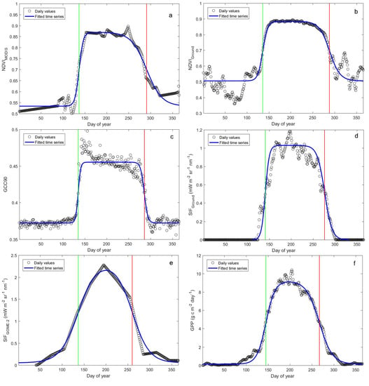
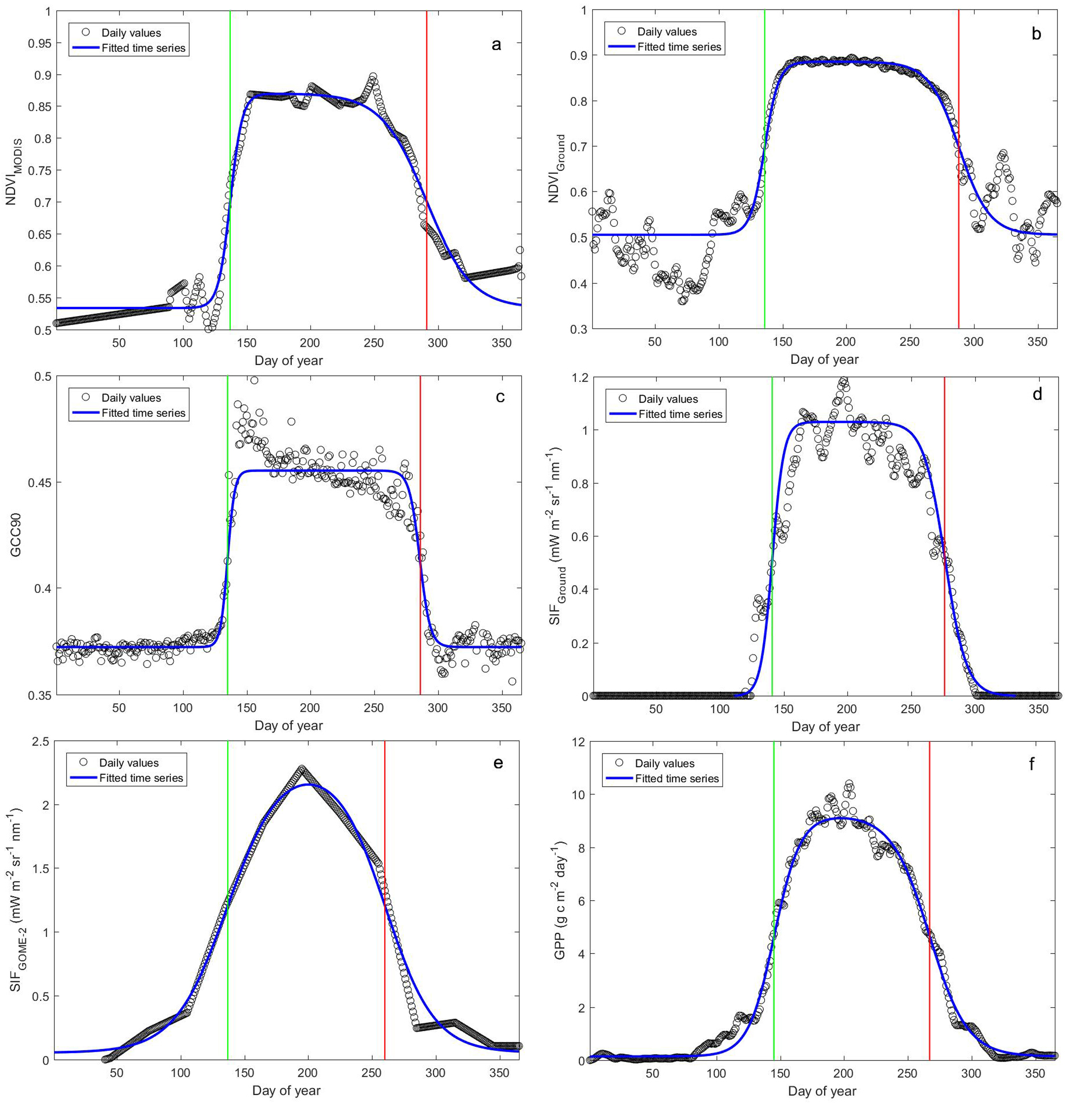
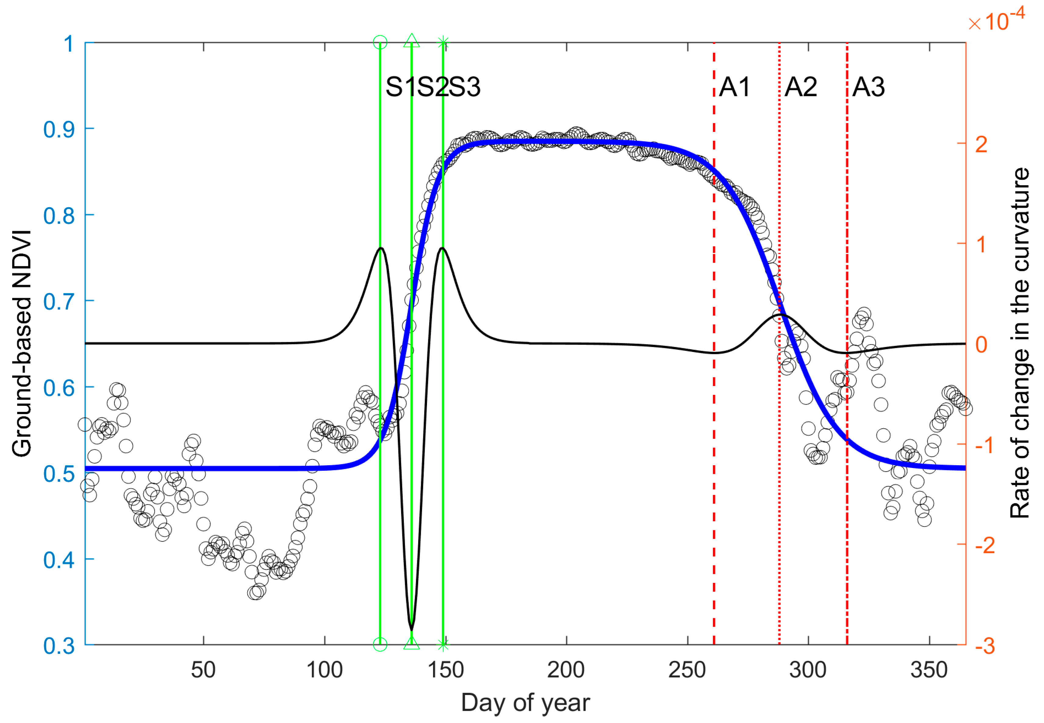
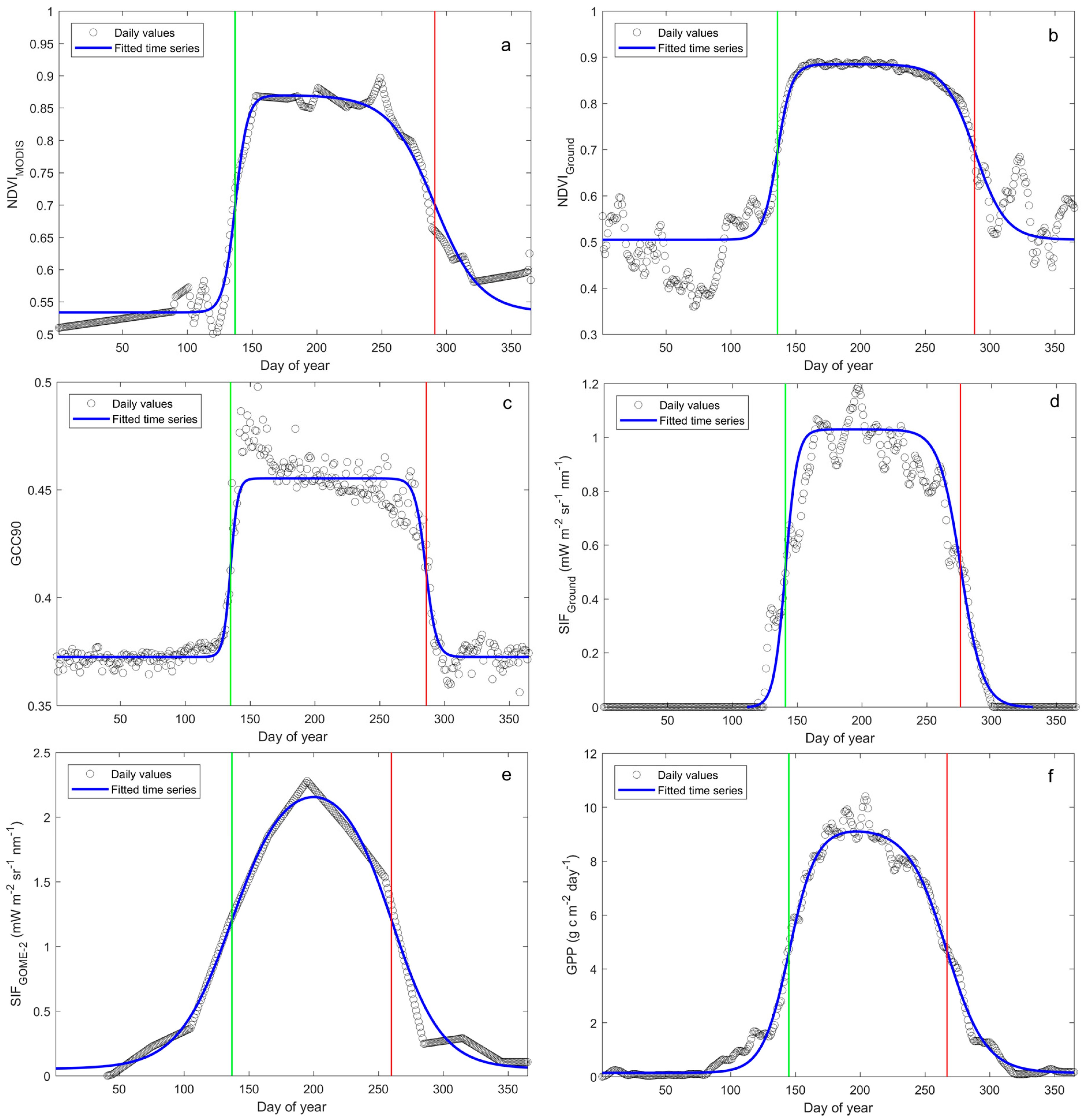
3.1. Phenology Derived from Reflectance-Based Indices

In this section, we compare phenological transition dates derived from three reflectance-based indices: GCC90, MODIS NDVI (NDVIMODIS) and the ground-based NDVI sensor (NDVIGround). The two NDVI data remain at a stable level around 0.5 during the dormant period (Figure 2a,b) because their footprints are relatively large and thus they also reflect impacts from evergreen vegetation within the corresponding pixel. Compared to rapid increases during the leaf development phase in the spring, the two NDVI data show a relatively slower decline in the period of leaf senescence phase in the autumn (Figure 2a,b). This long tail phenomenon can be partially explained by the contribution from newly fallen leaves on the ground [61]. In contrast, GCC90 demonstrates a more rapid change in both rising and falling parts of the seasonal trajectory (Figure 2c) and it shows a clear peak at the end of spring, which can be explained by seasonal variations in foliage pigments [15].
Among these three reflectance-based indices, GCC90 shows the smallest MAE compared to GPP in both spring and autumn (Table 2), highlighting its potential in predicting the GPP-based phenology events. Its strong synchronicity with GPP agrees well with a recent study which reported GCC had a good performance to predict the GPP-based seasons [62]. The phenological transition dates extracted from the NDVIMODIS and NDVIGround are comparable to those from the GCC90 in the spring, especially for the middle of spring (S2), and autumn (A2), which are observed on about Day of Year (DOY) 136 and 288, respectively (Table 1). This finding is consistent with previous studies [13,62], which also supported that NDVI and green index had similar performance in estimating spring phenology metrics.
However, the other two autumn phenological metrics from the NDVIMODIS are largely different to those derived from GCC90 and NDVIGround: the start of autumn (A1) from NDVIMODIS occurred around 20 days earlier and the end of autumn (A3) occurred about 30 days later (Table 1). One weakness of spaceborne optical remote sensing likely explains these discrepancies: cloud cover may significantly reduce its usable observations. High frequent clouds in September and October 2014 may cause many missing values and the temporal interpolation may shift the position of A1 to the left and A3 to the right. It also exhibits the stable performance of using the date of half-maximum values to predict dates of the middle of spring (S2) and autumn (A2), especially under strong noisy conditions.
The autumn phenological metrics derived from the reflectance-based time series lagged significantly compared to GPP, although their performance is good for the spring phenological metrics. For example, the GPP-based A2 in 2014 occurred 20, 21 and 24 days ahead compared to GCC90, NDVIGround and NDVIMODIS, respectively (Table 1). The multiyear comparison (Tables S1–S3 and S6) also confirms that these three reflectance-based data tend to provide significant later transition dates (A2) (p < 0.05). This lagged pattern is consistent with previous studies showing that green indices [51,62] and NDVI-based [19] methods tend to estimate a prolonged growing season, usually retrieving later autumn offset.

3.2. Phenology Estimated from In Situ Reflectance-Based Indices and SIF

In this section, we compare the phenology estimated from three in situ observations including GCC90, NDVIGround and ground-based SIF data (SIFGround). Since all these measurements were collected only a few meters above the canopy, and because their high temporal frequencies, the effects of forest type heterogeneity and temporal composite are less pronounced.
Among these three in situ data, SIFGround shows the best synchronicity with the tower-based GPP (Table 2) with a MAE value of 0.08 and 0.07 in in the spring and autumn seasons, respectively. In contrast, NDVIGround demonstrates the worst synchronicity with GPP with a MAE value of larger than 0.3 in the both spring and autumn seasons (Table 2). Compared to the other two in situ reflectance-based data, SIFGround exhibits faster changes in both spring development and autumn senescence (Figure 2d). Among these three, SIFGround demonstrates the best capacity to detect the GPP-based phenological events in both the spring and fall seasons: its S2 occurs only three days earlier than the GPP time series, while the other two time series yield earlier dates of S2 by longer than one week (Table 1). Similarly, the estimated A2 date from SIFGround is biased by only of six days later compared to GPP, while these dates in both GCC90 and SIFGround are more than 20 days later (Table 1). We also found that SIFGround shows a relatively better performance in estimating the rest of phenological metrics (S1, S3, A1 and A3), but discrepancies still exist (Table 1). The two-year comparison using measurements in 2014 and 2015 also shows that SIFGround provides similar S2 and A2 as GPP (Tables S4 and S6). Especially, SIFGround provides a clearly better estimation of A2 compared to GCC90 and NDVIGround.

3.3. Phenology Estimated from Satellite-Based NDVI and SIF

In this section, we assess the phenological transition dates derived from two satellite-based products including SIF740 retrieved from GOME-2 (SIFGOME-2) and NDVIMODIS. Because both have coarse spatial resolutions, the large field of view of these sensors may include considerable landscape heterogeneity. Due to the contribution from evergreen forest and mixed forest (Table 1), NDVIMODIS of deciduous forest still shows relative high values in the dormant season, and SIFGOME-2 detects photosynthetic activities in the very early spring (Figure 2a,e).
The start of spring (S1) determined from SIFGOME-2 occurs more than one month earlier than those from the NDVIMODIS and GPP time series (Table 1). The springtime rise in SIFGOME-2 is the earliest among all the time series. GOME-2 data are characterized by the large field of view of its sensor and coarse temporal resolution. The former feature may cause them contain signals from mixed vegetation. For the half-degree grid cell surrounding Harvard Forest, evergreen forest and mixed forest account for 25% and 16% (Table 1), which makes SIFGOME-2 still receive SIF emission in the dormant season (Figure 2e). Similarly, understory component with an earlier greenness may also lead to an early onset of spring in SIFGOME-2. All these factors more or less explain why S1 from SIFGOME-2 occurred very early in 2014 (Table 1). In addition, the length of their maturity period (A1-S3) is clearly different from that derived from the GPP data, with 28 days longer in NDVIMODIS and 36 days shorter in SIFGOME-2 (Table 1, Figure 2e). Remotely sensed datasets typically use values with the best quality within each time step to compose time series. Without information of date used in temporal composite, linear interpolation may cause large uncertainties in generating daily time series. Especially, the monthly time step of GOME-2 data may result in at most two-month bias in estimating these phenological metrics. However, the two satellite data and tower-based GPP produce the similar dates of middle of spring (S2), with an estimate of seven days earlier for both SIFGOME-2 and NDVIMODIS compared to GPP data (Table 1). It again shows the scheme using half-maximum values provides a good resistance to noises induced by spatial heterogeneity.
Although the spatial and temporal resolutions of SIFGOME-2 are coarse, it provides a better estimation of the autumn phenological metrics compared to NDVIMODIS. For example, the middle of fall (A2) derived from SIFGOME-2 is only seven days earlier compared to GPP observations, while the estimated A2 from NDVIMODIS is more than three weeks later (Table 1). The multi-year comparison (Tables S3, S5 and S6) using the data during the period of 2007–2015 also shows that: (1) SIFGOME-2 may cause large uncertainties in predicting the dates of start/end of the spring and autumn seasons (S1, S3, A1 and A3); and (2) both SIFGOME-2 and NDVIMODIS can provide close estimation of the date of S2 with respect to the GPP data and SIFGOME-2 can produce better estimation of the date of A2 than the latter.

3.4. Phenology Estimated from Satellite- and Ground-Based SIF

We compare dates of the phenophase transitions estimated from the two SIF data including SIFGOME-2 (740 nm) and SIFGround (760 nm) in this section. Although SIF radiance are at different wavelengths in these two data, the previous study [39] which was also implemented at Harvard Forest has shown that their measurements are highly linear correlated (Figure S1). Thus, their differences in the SIF wavelengths should have a minimal effect on extracting the phenological metrics.
The temporal pattern of SIFGOME-2 is inconsistent with in situ SIFGround in some aspects. SIFGround shows a sharp springtime rise (within 20 days) and autumn decline (within 30 days). In contrast, SIFGOME-2 shows slower rates in both the rising and the falling part of the seasonal trajectory (Figure 2e). In comparison to SIFGround, SIFGOME-2 also exhibits a shorter period of the summer plateau due to the later S3 and earlier A1 (Figure 2e). Again, these discrepancies can be explained by their difference in their spatial and temporal resolutions.
Although SIFGOME-2 and SIFGround are largely different in spatial and temporal resolutions, their estimations of dates of S2 show an only four-day difference and both are close to the S2 from the GPP with an earlier estimation of three and seven days, respectively (Table 1). In the autumn, SIFGOME-2 and SIFGround estimate dates of A2 by seven days earlier and six days later than that of the GPP time series, respectively (Table 1). Due to its high temporal and spatial resolutions, SIFGround can provide similar estimations of S1, S3, A1 and A3 to those from the GPP data (Table 1), whereas the estimates from SIFGOME-2 clearly deviate from the GPP observations. Furthermore, the comparison using SIFGOME-2 and SIFGround data during 2014–2015 also confirms that both SIFGOME-2 and SIFGround are good predictors of S2, and SIFGround can further estimate A2 with a better accuracy (Table S4).

4. Discussion

By showing the roles of biophysical properties and meteorological variables in affecting phenology metrics, we explain why SIF emission has a better performance in estimate the GPP-based phenological metrics in both spring and autumn seasons. In addition, we explore the effects of spatial and temporal resolutions on phenology derived from satellite and in situ SIF observations.

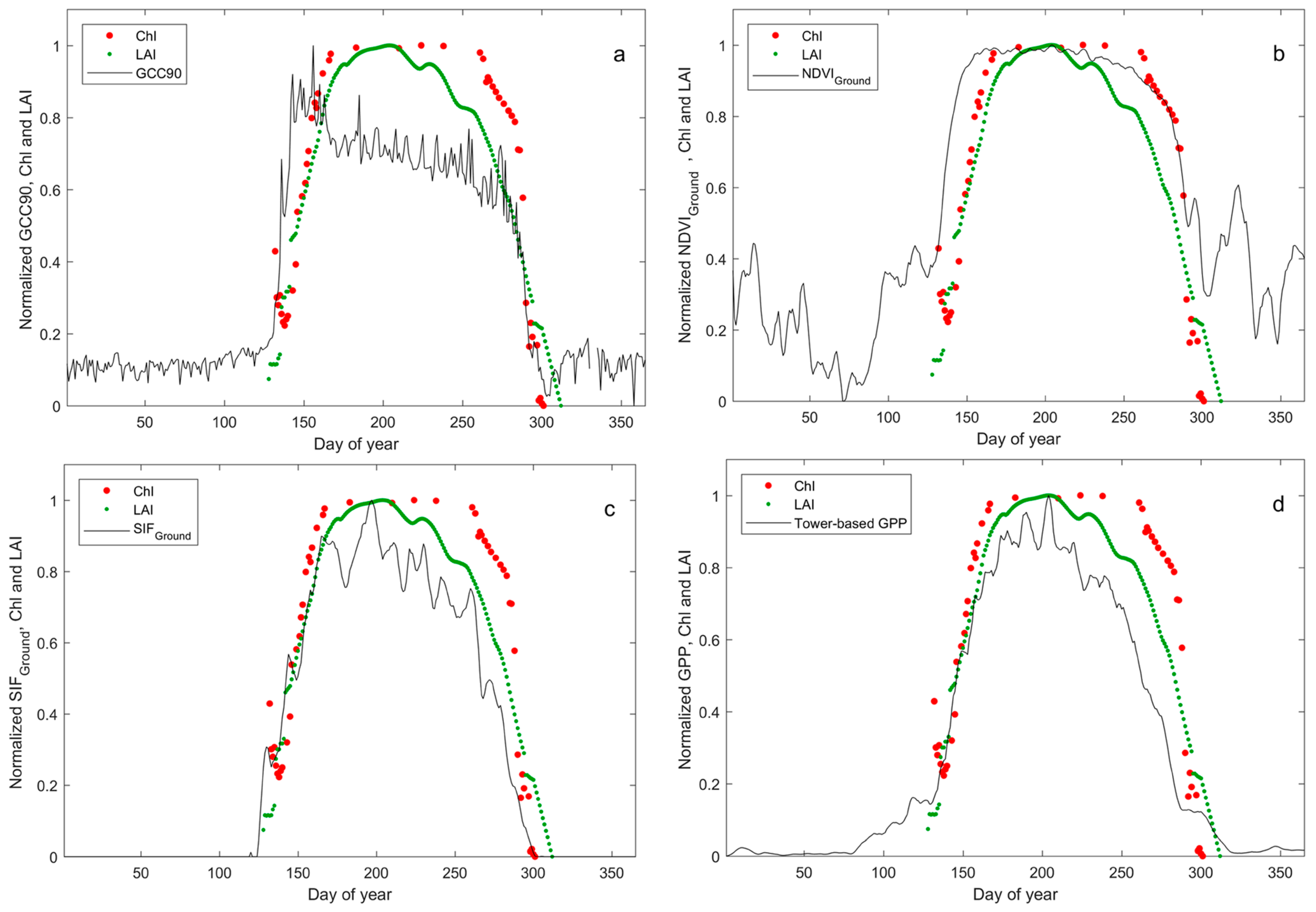
4.1. Effects of Biophysical Properties on Estimating Phenology

In this section, we discuss the roles of two physiological properties, LAI and Chl, in determining the plant phenological events. We use the time series from three ground-based sensors including GCC90, NDVIGround and SIFGround. Because all these sensors are near ground surface and collect measurements with high temporal frequencies, negative influences from cloud and landscape heterogeneity can be effectively suppressed.
The temporal trajectory of GPP is highly consistent with LAI and Chl in the spring season (Figure 3). The statistical analysis also supports that GPP is more synchronous with the two physiological properties than meteorological factors including air temperature and Photosynthetically Active Radiation (PAR, μmol photons m−2 s−1) during the spring period: LAI and Chl have MAE values less than 0.10 with respect to GPP in the spring, whereas MAE values between GPP and the two meteorological variables are more than 0.25 (Table 3). It shows that: (1) GPP-based phenological transition dates in the spring are more regulated by LAI and Chl than the two meteorological factors; and (2) phenological indicators which can track seasonal variations of these two plant physiological properties should also have a potential to predict the GPP-based spring phenology well.
Previous studies [54,63] showed that GCC90 is highly correlated with both LAI and Chl. Our results also confirm that GCC90 generally follows the temporal patterns of LAI and Chl in both spring and autumn periods (Figure 3a), which explains why GCC90 can estimate the middle of spring (S2) well (Table 3). However, we found a clear saturation phenomenon: GCC90 stops increasing when LAI and Chl exceed their thresholds (Figure 3a). It is one of the important reasons why there are discrepancies in estimating the other two springtime phenology metrics (S1 and S3) using GCC90. Although NDVIGround also generally follows the pattern of LAI and Chl, its estimated spring onset is earlier (Figure 3b) compared to LAI and Chl, probably due to its relative large footprint. It also partially explains why NDVIGround produces an earlier S2 than GPP (Table 1). Compared to the GCC90 and NDVIGround, SIFGround is more closely with these two properties in the leaf development stage (Figure 3c). SIFGround shows the lowest MAE values with LAI and Chl in the spring season (Table 3), which supports that it is strongly synchronous with the physiological properties in the spring season.
Both GCC90 and NDVI, similar to many other reflectance-based data, are designed to capture variations in selected physiological properties such as greenness, LAI and Chl. Because photosynthesis is largely regulated by these properties in the spring, GCC90 and NDVI have a good potential to track GPP-based phenology metrics in the spring well if the impact of spatial heterogeneity and coarse temporal resolution can be effectively reduced. Furthermore, SIF has a more direct link with photosynthesis activities such that it has a good performance in estimating GPP-based phenology in the spring as well.
On the contrary, we found an obvious decouple between these two physiological properties and photosynthesis rate in the fall offset season (Figure 3d). LAI and Chl show a clear lag behind GPP: GPP start dropping on DOY 235, while autumn leaf Chl reduction and LAI decline begins by about 15 and 8 days later, respectively. In addition, LAI and Chl have much larger MAE values relative to GPP data in the fall season compared to the spring season (Table 3). It suggests that the two physiological properties are not good indicators of GPP-based transition dates in the autumn. The decouple between the plant physiological properties (e.g., LAI and Chl) and photosynthesis rate in the fall season is the main reason for the poor performance of reflectance-based data in estimating the GPP-based autumn metrics.
SIFGround does not follow the trends of LAI and Chl in the fall as it does in the spring (Figure 3d). However, SIFGround still shows a strong similarity with GPP in the whole autumn season (Figure 3d, Table 3). Following the decline trend of GPP, SIF starts to decrease almost simultaneously even though both LAI and Chl still remain at a relatively high level (Figure 3c). It suggests that SIFGround tracks the GPP-based fall phenology through factors other than LAI and Chl (see below).

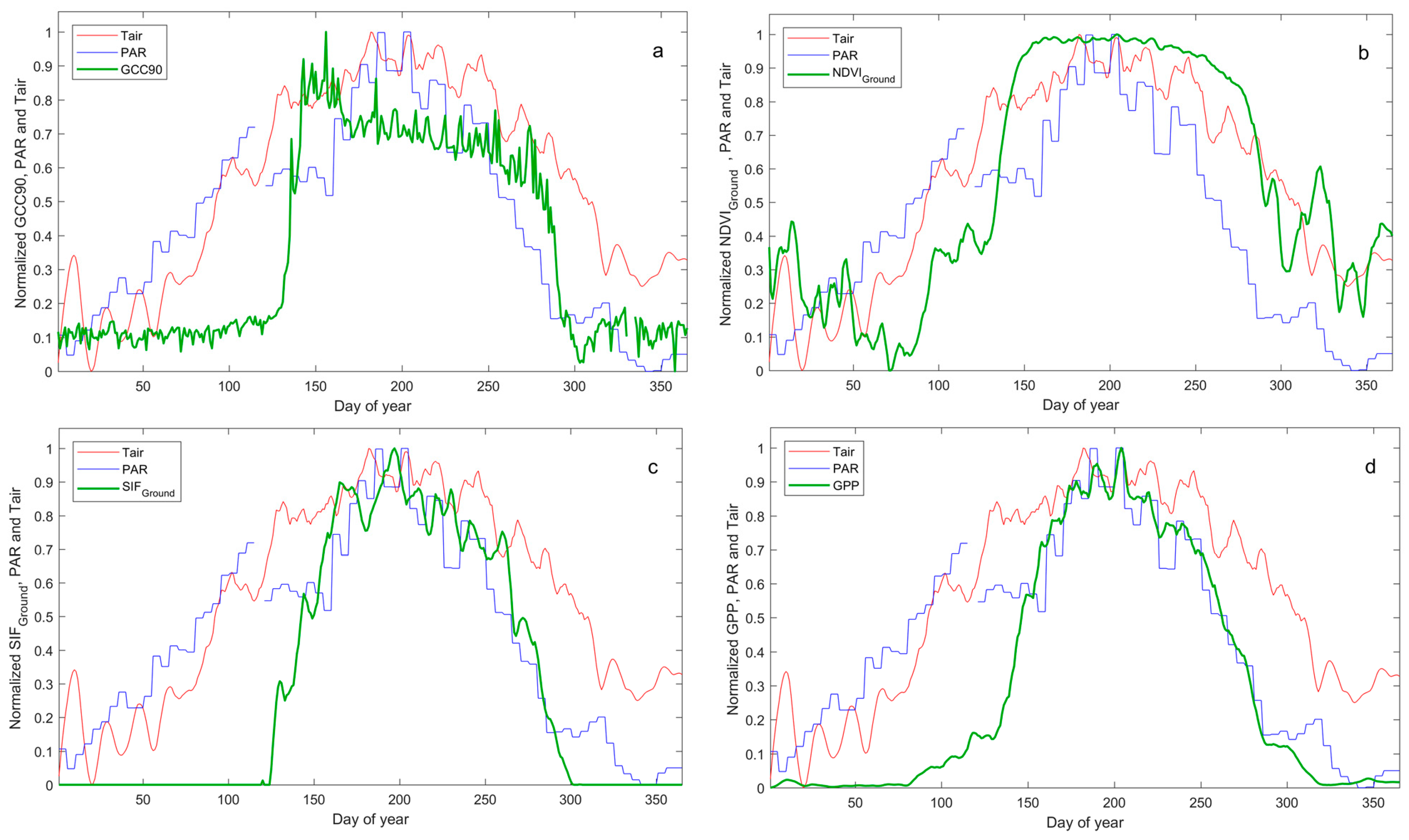
4.2. Effects of Meteorological Variables on Estimating Phenology

In this section, we examine effects of two meteorological variables including air temperature (Tair) and PAR on phenological transition dates using the three in situ observations (i.e., GCC90, NDVIGround and SIFGround) and tower-based GPP. Both Tair and PAR start to increase much earlier than the in situ time series and tower-based GPP (Figure 4). In comparison to LAI and Chl, both meteorological variables show much larger MAEs compared to GPP data in the spring (Table 3). It suggests Tair and PAR may not be direct factors determining GPP variations in the springtime in 2014, although these meteorological variables play as prerequisites of spring onset [64].
Again, Tair plays a limited role in determining the autumn phenology metrics in 2014: the autumn evolution of Tair lags much behind that of the other four time series (Figure 4). In comparison to Tair, PAR demonstrates a much earlier and faster decline trend (Figure 4). It is important to note these four time series show different responses to the drop of PAR: GCC90 and NDVIGround show a delayed response to variations in PAR, while the SIFGround and GPP data closely follow the decreasing trend of PAR (Figure 3). Particularly, PAR and GPP show the highest synchronicity with each other with a MAE of only 0.09 (Table 3), which indicates that the GPP in the fall season is limited by the amount of PAR.
In the autumn, solar radiation declines first, photosynthesis activities are immediately suppressed and then physiological traits decrease as a consequence of low carbon uptake. In other words, a good autumn phenology indicator should be able to account for effects of meteorological factors including PAR on GPP. All the reflectance-based data which use reflected signals as proxies to track photosynthesis activities actually capture subsequent consequences of decrease in GPP such that the autumn phenological metrics derived from them tend to lag after those from GPP time series. In contrast, SIF is a byproduct of photosynthetic activity and it can respond immediately to variations in photosynthesis caused by all possible factors including PAR. It explains why SIFGround has an advantage in estimating GPP-based phenology over NDVIGround and GCC90 in the fall season.
Our finding is consistent with a recent study [20] which found that photosynthesis may already significantly decrease before the onset of yellowing in the autumn. In fact, carbon uptake is mainly driven by variations in solar radiation in many mid-to-high latitude ecosystems such as temperate forests, particularly after summer solstice [65]. Reflectance-based data may cause later estimations of autumn phenological metrics in these ecosystems [20].

4.3. Effects of Spatial and Temporal Resolutions on SIF-Based Phenology

Numerous previous studies have shown phenology derived from optical satellite data could be subjected to coarse temporal resolution and landscape heterogeneity [21,23,66]. By comparison with SIFGround, we also found that phenological metrics from the GOME-2 SIF likely contain large uncertainties due to its low spatial and temporal resolutions (see Section 3.4). Vegetation understory may start to green more than three weeks earlier than forest canopy [67]. Due to its coarse spatial resolution, a large contribution of understory phenology may significantly shift these phenological events. Particularly, we found that the start and end of spring/autumn (S1, S3, A1 and A3) derived from GOME-2 SIF may contain large biases, while dates of the middle of spring/autumn (S2 and A2) can be still estimated from them reasonably well. Therefore, GOME-2 SIF is still useful in predicting the GPP-based phenology, especially in the autumn season. Although our analysis showed that SIF measurements retrieved from current satellites were too coarse for phenology studies, future space-borne sensors such as Fluorescence Explorer (FLEX, [68]) will provide SIF observations with higher spatial and temporal resolutions, such that variations in phenology could be better monitored through the upcoming sensors.
The temporal resolution of satellite data is another important factor affecting the performance of GOME-2 SIF in capturing phenological events [69]. We show that the low temporal resolution of GOME-2 SIF may also lead to large uncertainties in estimating phenological metrics. In addition to improving temporal resolution of future SIF satellites, a previous study [22] showed that exact observation dates of values used in temporal composition can help to reduce errors associated with its coarse temporal resolution. Considering temporal composite is usually necessary in processing remote sensing data, retaining exact day of acquisition is highly needed in future satellite SIF products to improve accuracy of remote sensing phenological indicators.
Among all the time series, SIFGround demonstrates the best capacity to predict the GPP-based phenology in both the spring and fall seasons. Although the effects of spatial and temporal resolutions on the performance of SIF in estimating the phenological metrics need to be analyzed in much more detail, our results clearly show that there is a great need to combine both site-level and satellite-based SIF observations in future phenology studies.

5. Conclusions

In this study, we assessed the consistencies and discrepancies of phenology estimated from reflectance-based and SIF observations and explored their advantages and disadvantages. We found: (1) duration of canopy greenness has a relatively weak correlation with the carbon uptake period in the study site such that a systematic later bias exists between the phenology markers derived from reflectance-based data and those from GPP time series, which is especially true in the autumn season; (2) SIF has a more direct connection with the seasonality of photosynthesis and it has a stronger ability to track photosynthetic capacity than the reflectance-based time series, particularly for the phenological markers associated with the autumn season; and (3) both physiological properties and meteorological variables could be the direct factors controlling phenological stages; the good performance of SIF emission in estimating the phenological metrics relies on its ability to track both of them. Our results show that there is a need to combine site-level and satellite-based SIF observations in future phenology studies, especially when satellite-based data with better resolutions FLEX are available. Furthermore, the lag in phenology derived from the reflectance-based data revealed in this study can also be used to rectify related phenology estimates or re-calibrate models that predict phenology based on reflectance-based data.

Supplementary Materials

The following are available online at https://0-www-mdpi-com.brum.beds.ac.uk/2072-4292/10/6/932/s1, Figure S1: Comparison between the smoothed GOME-2-derived SIF and ground-measured SIF (black) time series at the Harvard Site in 2014. The original GOME-2-derived SIF emission at 740 nm (red) and converted SIF emission at 760 nm (blue) are shown. Ground-measured SIF is for 760 nm. The time step is daily. Figure S2: The land cover distribution (NLCD) in the footprints of different measurements: (a) the GOME-2 scene; and (b) GPP (big circle), MODIS NDVI (NDVIMODIS, black rectangle), NDVI sensor (NDVIGround, blue rectangle) and GCC90 (small red circle). The footprint of ground-based SIF emission (SIFGround) only accounts for about 4% of the size of GCC90. Table S1: The phenological metrics derived from the 90th percentile of the green chromatic coordinates (GCC90) at the Harvard Forest site during 2008–2015. S1, S2 and S3 represent the start of spring, middle of spring and end of spring, respectively. A1, A2 and A3 stand for the start of autumn, middle of autumn and end of autumn, respectively. Table S2: The phenological metrics derived from the ground-based NDVI (NDVIGround) at the Harvard Forest site in 2014 and 2015. S1, S2 and S3 represent the start of spring, middle of spring and end of spring, respectively. A1, A2 and A3 stand for the start of autumn, middle of autumn and end of autumn, respectively. Table S3: The phenological metrics derived from the MODIS NDVI (NDVIMODIS) at the Harvard Forest site during 2007–2015. S1, S2 and S3 represent the start of spring, middle of spring and end of spring, respectively. A1, A2 and A3 stand for the start of autumn, middle of autumn and end of autumn, respectively. Table S4: The phenological metrics derived from the ground-based SIF (SIFGround) at the Harvard Forest site in 2014 and 2015. S1, S2 and S3 represent the start of spring, middle of spring and end of spring, respectively. A1, A2 and A3 stand for the start of autumn, middle of autumn and end of autumn, respectively. Table S5: The phenological metrics derived from the GOME-2 SIF (SIFGOME-2) at the Harvard Forest site during 2007–2015. S1, S2 and S3 represent the start of spring, middle of spring and end of spring, respectively. A1, A2 and A3 stand for the start of autumn, middle of autumn and end of autumn, respectively. Table S6: The phenological metrics derived from gross primary production (GPP) at the Harvard Forest site during 2007–2015. S1, S2 and S3 represent the start of spring, middle of spring and end of spring, respectively. A1, A2 and A3 stand for the start of autumn, middle of autumn and end of autumn, respectively.

Author Contributions

X.L. and Z.L. conceived and designed the study, and interpreted the results; X.L. carried out the analyses and wrote the paper; Y.L., Y.Z., S.A. and J.T. contributed to the manuscript revision; and Z.L. and J.T. made important contributions to the field experiments.

Funding

This research was supported by U. S. Department of Energy Office of Biological and Environmental Research Grant DE-SC0006951, National Science Foundation Grants DBI 959333 and AGS-1005663, and the University of Chicago and the MBL Lillie Research Innovation Award to Jianwu Tang and China Scholarship Council No. 201506190095 to Z. Liu. Xiaoliang Lu was also supported by the open project grant (LBKF201701) of Key Laboratory of Land Surface Pattern and Simulation, Chinese Academy of Sciences.

Acknowledgments

We would like to thank Harvard Forest for providing site and logistic support during our research. The water flux data were downloaded from the Harvard Forest data archive (PI: J. William Munger). We thank the National PhenoCam Network for managing the PhenoCam.

Conflicts of Interest

The authors declare no conflict of interest.

References

  1. Parmesan, C.; Yohe, G. A globally coherent fingerprint of climate change impacts across natural systems. Nature 2003, 421, 37–42. [Google Scholar] [CrossRef] [PubMed]
  2. White, M.A.; Thornton, P.E.; Running, S.W. A continental phenology model for monitoring vegetation responses to interannual climatic variability. Glob. Biogeochem. Cycle 1997, 11, 217–234. [Google Scholar] [CrossRef] [Green Version]
  3. Chuine, I. A unified model for budburst of trees. J. Theor. Biol. 2000, 207, 337–347. [Google Scholar] [CrossRef] [PubMed]
  4. Yang, X.; Mustard, J.F.; Tang, J.W.; Xu, H. Regional-scale phenology modeling based on meteorological records and remote sensing observations. J. Geophys. Res.-Biogeosci. 2012, 117, 18. [Google Scholar] [CrossRef]
  5. Tang, J.W.; Korner, C.; Muraoka, H.; Piao, S.L.; Shen, M.G.; Thackeray, S.J.; Yang, X. Emerging opportunities and challenges in phenology: A review. Ecosphere 2016, 7, 17. [Google Scholar] [CrossRef]
  6. Richardson, A.D.; Braswell, B.H.; Hollinger, D.Y.; Jenkins, J.P.; Ollinger, S.V. Near-surface remote sensing of spatial and temporal variation in canopy phenology. Ecol. Appl. 2009, 19, 1417–1428. [Google Scholar] [CrossRef] [PubMed]
  7. Richardson, A.D.; Black, T.A.; Ciais, P.; Delbart, N.; Friedl, M.A.; Gobron, N.; Hollinger, D.Y.; Kutsch, W.L.; Longdoz, B.; Luyssaert, S.; et al. Influence of spring and autumn phenological transitions on forest ecosystem productivity. Philos. Trans. R. Soc. B Biol. Sci. 2010, 365, 3227–3246. [Google Scholar] [CrossRef] [PubMed] [Green Version]
  8. Zhang, X.Y.; Friedl, M.A.; Schaaf, C.B.; Strahler, A.H.; Hodges, J.C.F.; Gao, F.; Reed, B.C.; Huete, A. Monitoring vegetation phenology using MODIS. Remote Sens. Environ. 2003, 84, 471–475. [Google Scholar] [CrossRef]
  9. Zhang, X.Y.; Friedl, M.A.; Schaaf, C.B.; Strahler, A.H.; Liu, Z. Monitoring the response of vegetation phenology to precipitation in Africa by coupling MODIS and TRMM instruments. J. Geophys. Res. Atmos. 2005, 110, 14. [Google Scholar] [CrossRef]
  10. Zhang, X.Y.; Friedl, M.A.; Schaaf, C.B. Global vegetation phenology from moderate resolution imaging spectroradiometer (MODIS): Evaluation of global patterns and comparison with in situ measurements. J. Geophys. Res. Biogeosci. 2006, 111, 14. [Google Scholar] [CrossRef]
  11. Liang, L.; Schwartz, M.D.; Wang, Z.S.; Gao, F.; Schaaf, C.B.; Tan, B.; Morisette, J.T.; Zhang, X.Y. A cross comparison of spatiotemporally enhanced springtime phenological measurements from satellites and ground in a northern US Mixed forest. IEEE Trans. Geosci. Remote Sens. 2014, 52, 7513–7526. [Google Scholar] [CrossRef]
  12. Shuai, Y.M.; Schaaf, C.; Zhang, X.Y.; Strahler, A.; Roy, D.; Morisette, J.; Wang, Z.S.; Nightingale, J.; Nickeson, J.; Richardson, A.D.; et al. Daily MODIS 500 m reflectance anisotropy direct broadcast (db) products for monitoring vegetation phenology dynamics. Int. J. Remote Sens. 2013, 34, 5997–6016. [Google Scholar] [CrossRef]
  13. Richardson, A.D.; Jenkins, J.P.; Braswell, B.H.; Hollinger, D.Y.; Ollinger, S.V.; Smith, M.L. Use of digital webcam images to track spring green-up in a deciduous broadleaf forest. Oecologia 2007, 152, 323–334. [Google Scholar] [CrossRef] [PubMed]
  14. Richardson, A.D.; Hufkens, K.; Milliman, T.; Aubrecht, D.M.; Chen, M.; Gray, J.M.; Johnston, M.R.; Keenan, T.F.; Klosterman, S.T.; Kosmala, M.; et al. Tracking vegetation phenology across diverse North American biomes using phenocam imagery. Sci. Data 2018, 5, 24. [Google Scholar] [CrossRef] [PubMed]
  15. Sonnentag, O.; Hufkens, K.; Teshera-Sterne, C.; Young, A.M.; Friedl, M.; Braswell, B.H.; Milliman, T.; O'Keefe, J.; Richardson, A.D. Digital repeat photography for phenological research in forest ecosystems. Agric. For. Meteorol. 2012, 152, 159–177. [Google Scholar] [CrossRef]
  16. Tucker, C.J. Red and photographic infrared linear combinations for monitoring vegetation. Remote Sens. Environ. 1979, 8, 127–150. [Google Scholar] [CrossRef] [Green Version]
  17. Wu, C.Y.; Peng, D.L.; Soudani, K.; Siebicke, L.; Gough, C.M.; Arain, M.A.; Bohrer, G.; Lafleur, P.M.; Peichl, M.; Gonsamo, A. Land surface phenology derived from normalized difference vegetation index (NDVI) at global Fluxnet sites. Agric. For. Meteorol. 2017, 233, 171–182. [Google Scholar] [CrossRef]
  18. Yang, H.L.; Yang, X.; Heskel, M.; Sun, S.C.; Tang, J.W. Seasonal variations of leaf and canopy properties tracked by ground-based NDVI imagery in a temperate forest. Sci. Rep. 2017, 7, 10. [Google Scholar] [CrossRef] [PubMed]
  19. Churkina, G.; Schimel, D.; Braswell, B.H.; Xiao, X.M. Spatial analysis of growing season length control over net ecosystem exchange. Glob. Chang. Biol. 2005, 11, 1777–1787. [Google Scholar] [CrossRef]
  20. Jeong, S.J.; Schimel, D.; Frankenberg, C.; Drewry, D.T.; Fisher, J.B.; Verma, M.; Berry, J.A.; Lee, J.E.; Joiner, J. Application of satellite solar-induced chlorophyll fluorescence to understanding large-scale variations in vegetation phenology and function over northern high latitude forests. Remote Sens. Environ. 2017, 190, 178–187. [Google Scholar] [CrossRef]
  21. Zhang, X.Y.; Wang, J.M.; Gao, F.; Liu, Y.; Schaaf, C.; Friedl, M.; Yu, Y.Y.; Jayavelu, S.; Gray, J.; Liu, L.L.; et al. Exploration of scaling effects on coarse resolution land surface phenology. Remote Sens. Environ. 2017, 190, 318–330. [Google Scholar] [CrossRef]
  22. Kross, A.; Fernandes, R.; Seaquist, J.; Beaubien, E. The effect of the temporal resolution of NDVI data on season onset dates and trends across Canadian broadleaf forests. Remote Sens. Environ. 2011, 115, 1564–1575. [Google Scholar] [CrossRef]
  23. Ahl, D.E.; Gower, S.T.; Burrows, S.N.; Shabanov, N.V.; Myneni, R.B.; Knyazikhin, Y. Monitoring spring canopy phenology of a deciduous broadleaf forest using MODIS. Remote Sens. Environ. 2006, 104, 88–95. [Google Scholar] [CrossRef] [Green Version]
  24. Daumard, F.; Champagne, S.; Fournier, A.; Goulas, Y.; Ounis, A.; Hanocq, J.F.; Moya, I. A field platform for continuous measurement of canopy fluorescence. IEEE Trans. Geosci. Remote Sens. 2010, 48, 3358–3368. [Google Scholar] [CrossRef]
  25. Walther, S.; Voigt, M.; Thum, T.; Gonsamo, A.; Zhang, Y.G.; Kohler, P.; Jung, M.; Varlagin, A.; Guanter, L. Satellite chlorophyll fluorescence measurements reveal large-scale decoupling of photosynthesis and greenness dynamics in boreal evergreen forests. Glob. Chang. Biol. 2016, 22, 2979–2996. [Google Scholar] [CrossRef] [PubMed] [Green Version]
  26. Frankenberg, C.; Fisher, J.B.; Worden, J.; Badgley, G.; Saatchi, S.S.; Lee, J.E.; Toon, G.C.; Butz, A.; Jung, M.; Kuze, A.; et al. New global observations of the terrestrial carbon cycle from GOSAT: Patterns of plant fluorescence with gross primary productivity. Geophys. Res. Lett. 2011, 38, 6. [Google Scholar] [CrossRef]
  27. Yang, X.; Tang, J.W.; Mustard, J.F. Beyond leaf color: Comparing camera-based phenological metrics with leaf biochemical, biophysical, and spectral properties throughout the growing season of a temperate deciduous forest. J. Geophys. Res. Biogeosci. 2014, 119, 181–191. [Google Scholar] [CrossRef] [Green Version]
  28. Frankenberg, C.; O'Dell, C.; Berry, J.; Guanter, L.; Joiner, J.; Kohler, P.; Pollock, R.; Taylor, T.E. Prospects for chlorophyll fluorescence remote sensing from the orbiting carbon observatory-2. Remote Sens. Environ. 2014, 147, 1–12. [Google Scholar] [CrossRef]
  29. Guanter, L.; Zhang, Y.G.; Jung, M.; Joiner, J.; Voigt, M.; Berry, J.A.; Frankenberg, C.; Huete, A.R.; Zarco-Tejada, P.; Lee, J.E.; et al. Global and time-resolved monitoring of crop photosynthesis with chlorophyll fluorescence. Proc. Natl. Acad. Sci. USA 2014, 111, E1327–E1333. [Google Scholar] [CrossRef] [PubMed] [Green Version]
  30. Zhang, Y.G.; Guanter, L.; Berry, J.A.; Joiner, J.; van der Tol, C.; Huete, A.; Gitelson, A.; Voigt, M.; Kohler, P. Estimation of vegetation photosynthetic capacity from space-based measurements of chlorophyll fluorescence for terrestrial biosphere models. Glob. Chang. Biol. 2014, 20, 3727–3742. [Google Scholar] [CrossRef] [PubMed] [Green Version]
  31. Damm, A.; Elbers, J.; Erler, A.; Gioli, B.; Hamdi, K.; Hutjes, R.; Kosvancova, M.; Meroni, M.; Miglietta, F.; Moersch, A.; et al. Remote sensing of sun-induced fluorescence to improve modeling of diurnal courses of gross primary production (GPP). Glob. Chang. Biol. 2010, 16, 171–186. [Google Scholar] [CrossRef] [Green Version]
  32. Damm, A.; Guanter, L.; Paul-Limoges, E.; van der Tol, C.; Hueni, A.; Buchmann, N.; Eugster, W.; Ammann, C.; Schaepman, M.E. Far-red sun-induced chlorophyll fluorescence shows ecosystem-specific relationships to gross primary production: An assessment based on observational and modeling approaches. Remote Sens. Environ. 2015, 166, 91–105. [Google Scholar] [CrossRef]
  33. Guan, K.Y.; Berry, J.A.; Zhang, Y.G.; Joiner, J.; Guanter, L.; Badgley, G.; Lobell, D.B. Improving the monitoring of crop productivity using spaceborne solar-induced fluorescence. Glob. Chang. Biol. 2016, 22, 716–726. [Google Scholar] [CrossRef] [PubMed]
  34. Yang, H.L.; Yang, X.; Zhang, Y.G.; Heskel, M.A.; Lu, X.L.; Munger, J.W.; Sun, S.C.; Tang, J.W. Chlorophyll fluorescence tracks seasonal variations of photosynthesis from leaf to canopy in a temperate forest. Glob. Chang. Biol. 2017, 23, 2874–2886. [Google Scholar] [CrossRef] [PubMed]
  35. Yang, X.; Tang, J.W.; Mustard, J.F.; Lee, J.E.; Rossini, M.; Joiner, J.; Munger, J.W.; Kornfeld, A.; Richardson, A.D. Solar-induced chlorophyll fluorescence that correlates with canopy photosynthesis on diurnal and seasonal scales in a temperate deciduous forest. Geophys. Res. Lett. 2015, 42, 2977–2987. [Google Scholar] [CrossRef] [Green Version]
  36. Luus, K.A.; Commane, R.; Parazoo, N.C.; Benmergui, J.; Euskirchen, E.S.; Frankenberg, C.; Joiner, J.; Lindaas, J.; Miller, C.E.; Oechel, W.C.; et al. Tundra photosynthesis captured by satellite-observed solar-induced chlorophyll fluorescence. Geophys. Res. Lett. 2017, 44, 1564–1573. [Google Scholar] [CrossRef] [Green Version]
  37. Lu, X.L.; Liu, Z.Q.; An, S.Q.; Miralles, D.G.; Maes, W.; Liu, Y.L.; Tang, J.W. Potential of solar-induced chlorophyll fluorescence to estimate transpiration in a temperate forest. Agric. For. Meteorol. 2018, 252, 75–87. [Google Scholar] [CrossRef]
  38. Schaaf, C.B.; Liu, J.; Gao, F.; Strahler, A.H. Aqua and Terra MODIS albedo and reflectance anisotropy products. In Land Remote Sensing and Global Environmental Change. NASA’s Earth Observing System and the Science of ASTER and MODIS; Ramachandran, B., Justice, C.O., Abrams, M.J., Eds.; Springer: New York, NY, USA, 2010; pp. 549–561. [Google Scholar]
  39. Schaaf, C.B.; Gao, F.; Strahler, A.H.; Lucht, W.; Li, X.W.; Tsang, T.; Strugnell, N.C.; Zhang, X.Y.; Jin, Y.F.; Muller, J.P.; et al. First operational BRDF, albedo NADIR reflectance products from MODIS. Remote Sens. Environ. 2002, 83, 135–148. [Google Scholar] [CrossRef]
  40. Joiner, J.; Guanter, L.; Lindstrot, R.; Voigt, M.; Vasilkov, A.P.; Middleton, E.M.; Huemmrich, K.F.; Yoshida, Y.; Frankenberg, C. Global monitoring of terrestrial chlorophyll fluorescence from moderate-spectral-resolution near-infrared satellite measurements: Methodology, simulations, and application to gome-2. Atmos. Meas. Tech. 2013, 6, 2803–2823. [Google Scholar] [CrossRef]
  41. Köhler, P.; Guanter, L.; Joiner, J. A linear method for the retrieval of sun-induced chlorophyll fluorescence from gome-2 and SCIAMACHY data. Atmos. Meas. Tech. 2015, 8, 2589–2608. [Google Scholar] [CrossRef]
  42. Baldocchi, D.D. Assessing the eddy covariance technique for evaluating carbon dioxide exchange rates of ecosystems: Past, present and future. Glob. Chang. Biol. 2003, 9, 479–492. [Google Scholar] [CrossRef]
  43. Munger, W.; Wofsy, S. Canopy-Atmosphere Exchange of Carbon, Water and Energy at Harvard Forest EMS Tower since 1991. Harv. For. Data Arch. HF004 2017. [Google Scholar] [CrossRef]
  44. Papale, D.; Reichstein, M.; Aubinet, M.; Canfora, E.; Bernhofer, C.; Kutsch, W.; Longdoz, B.; Rambal, S.; Valentini, R.; Vesala, T.; et al. Towards a standardized processing of net ecosystem exchange measured with eddy covariance technique: Algorithms and uncertainty estimation. Biogeosciences 2006, 3, 571–583. [Google Scholar] [CrossRef]
  45. Reichstein, M.; Falge, E.; Baldocchi, D.; Papale, D.; Aubinet, M.; Berbigier, P.; Bernhofer, C.; Buchmann, N.; Gilmanov, T.; Granier, A.; et al. On the separation of net ecosystem exchange into assimilation and ecosystem respiration: Review and improved algorithm. Glob. Chang. Biol. 2005, 11, 1424–1439. [Google Scholar] [CrossRef]
  46. Fry, J.; Xian, G.; Jin, S.; Dewitz, J.; Homer, C.; Yang, L.; Barnes, C.; Herold, N.; Wickham, J. Completion of the 2006 national land cover database for the conterminous United States. Photogramm. Eng. Remote Sens. 2011, 77, 858–864. [Google Scholar]
  47. Plascyk, J.A.; Gabriel, F.C. The Fraunhofer Line Discriminator MKII—An airborne instrument for precise and standardized ecological luminescence measurements. IEEE Trans. Instrum. Meas. 1975, 24, 306–313. [Google Scholar] [CrossRef]
  48. Meroni, M.; Busetto, L.; Colombo, R.; Guanter, L.; Moreno, J.; Verhoef, W. Performance of spectral fitting methods for vegetation fluorescence quantification. Remote Sens. Environ. 2010, 114, 363–374. [Google Scholar] [CrossRef]
  49. Zhao, F.; Guo, Y.Q.; Verhoef, W.; Gu, X.F.; Liu, L.Y.; Yang, G.J. A method to reconstruct the solar-induced canopy fluorescence spectrum from hyperspectral measurements. Remote Sens. 2014, 6, 10171–10192. [Google Scholar] [CrossRef]
  50. Gillespie, A.R.; Kahle, A.B.; Walker, R.E. Color enhancement of highly correlated images. 2. Channel ratio and chromaticity transformation techniques. Remote Sens. Environ. 1987, 22, 343–365. [Google Scholar] [CrossRef]
  51. Woebbecke, D.M.; Meyer, G.E.; Vonbargen, K.; Mortensen, D.A. Color indexes for weed identification under various soil, residue, and lighting conditions. Trans. ASAE 1995, 38, 259–269. [Google Scholar] [CrossRef]
  52. Mizunuma, T.; Koyanagi, T.; Mencuccini, M.; Nasahara, K.N.; Wingate, L.; Grace, J. The comparison of several colour indices for the photographic recording of canopy phenology of fagus crenata blume in eastern Japan. Plant Ecol. Divers. 2011, 4, 67–77. [Google Scholar] [CrossRef]
  53. Nagai, S.; Saitoh, T.M.; Noh, N.J.; Yoon, T.K.; Kobayashi, H.; Suzuki, R.; Nasahara, K.N.; Son, Y.; Muraoka, H. Utility of information in photographs taken upwards from the floor of closed-canopy deciduous broadleaved and closed-canopy evergreen coniferous forests for continuous observation of canopy phenology. Ecol. Inform. 2013, 18, 10–19. [Google Scholar] [CrossRef]
  54. Liu, Z.Q.; Hu, H.B.; Yu, H.; Yang, X.; Yang, H.L.; Ruan, C.X.; Wang, Y.; Tang, J.W. Relationship between leaf physiologic traits and canopy color indices during the leaf expansion period in an oak forest. Ecosphere 2015, 6, 9. [Google Scholar] [CrossRef]
  55. Zhang, X.Y.; Friedl, M.A.; Schaaf, C.B.; Strahler, A.H. Climate controls on vegetation phenological patterns in northern mid- and high latitudes inferred from MODIS data. Glob. Chang. Biol. 2004, 10, 1133–1145. [Google Scholar] [CrossRef]
  56. Hmimina, G.; Dufrene, E.; Pontailler, J.Y.; Delpierre, N.; Aubinet, M.; Caquet, B.; de Grandcourt, A.; Burban, B.; Flechard, C.; Granier, A.; et al. Evaluation of the potential of MODIS satellite data to predict vegetation phenology in different biomes: An investigation using ground-based NDVI measurements. Remote Sens. Environ. 2013, 132, 145–158. [Google Scholar] [CrossRef]
  57. Kato, S.; Komiyama, A. Spatial and seasonal heterogeneity in understory light conditions caused by differential leaf flushing of deciduous overstory trees. Ecol. Res. 2002, 17, 687–693. [Google Scholar] [CrossRef]
  58. Pellikka, P. Application of vertical skyward wide-angle photography and airborne video data for phenological studies of beech forests in the German Alps. Int. J. Remote Sens. 2001, 22, 2675–2700. [Google Scholar] [CrossRef]
  59. Elmore, A.J.; Guinn, S.M.; Minsley, B.J.; Richardson, A.D. Landscape controls on the timing of spring, autumn, and growing season length in mid-atlantic forests. Glob. Chang. Biol. 2012, 18, 656–674. [Google Scholar] [CrossRef]
  60. Testa, S.; Soudani, K.; Boschetti, L.; Mondino, E.B. MODIS-derived EVI, NDVI and WDRVI time series to estimate phenological metrics in French deciduous forests. Int. J. Appl. Earth Observ. Geoinform. 2018, 64, 132–144. [Google Scholar] [CrossRef]
  61. Nagler, P.L.; Daughtry, C.S.T.; Goward, S.N. Plant litter and soil reflectance. Remote Sens. Environ. 2000, 71, 207–215. [Google Scholar] [CrossRef]
  62. Toomey, M.; Friedl, M.A.; Frolking, S.; Hufkens, K.; Klosterman, S.; Sonnentag, O.; Baldocchi, D.D.; Bernacchi, C.J.; Biraud, S.C.; Bohrer, G.; et al. Greenness indices from digital cameras predict the timing and seasonal dynamics of canopy-scale photosynthesis. Ecol. Appl. 2015, 25, 99–115. [Google Scholar] [CrossRef] [PubMed] [Green Version]
  63. Nagai, S.; Maeda, T.; Gamo, M.; Muraoka, H.; Suzuki, R.; Nasahara, K.N. Using digital camera images to detect canopy condition of deciduous broad-leaved trees. Plant Ecol. Divers. 2011, 4, 79–89. [Google Scholar] [CrossRef]
  64. Piao, S.L.; Tan, J.G.; Chen, A.P.; Fu, Y.H.; Ciais, P.; Liu, Q.; Janssens, I.A.; Vicca, S.; Zeng, Z.Z.; Jeong, S.J.; et al. Leaf onset in the northern hemisphere triggered by daytime temperature. Nat. Commun. 2015, 6, 8. [Google Scholar] [CrossRef] [PubMed]
  65. Bauerle, W.L.; Oren, R.; Way, D.A.; Qian, S.S.; Stoy, P.C.; Thornton, P.E.; Bowden, J.D.; Hoffman, F.M.; Reynolds, R.F. Photoperiodic regulation of the seasonal pattern of photosynthetic capacity and the implications for carbon cycling. Proc. Natl. Acad. Sci. USA 2012, 109, 8612–8617. [Google Scholar] [CrossRef] [PubMed] [Green Version]
  66. White, K.; Pontius, J.; Schaberg, P. Remote sensing of spring phenology in northeastern forests: A comparison of methods, field metrics and sources of uncertainty. Remote Sens. Environ. 2014, 148, 97–107. [Google Scholar] [CrossRef]
  67. Augspurger, C.K.; Cheeseman, J.M.; Salk, C.F. Light gains and physiological capacity of understorey woody plants during phenological avoidance of canopy shade. Funct. Ecol. 2005, 19, 537–546. [Google Scholar] [CrossRef] [Green Version]
  68. Drusch, M.; Moreno, J.; Del Bello, U.; Franco, R.; Goulas, Y.; Huth, A.; Kraft, S.; Middleton, E.M.; Miglietta, F.; Mohammed, G.; et al. The FLuorescence EXplorer Mission Concept—ESA’s Earth Explorer 8. IEEE Trans. Geosci. Remote Sens. 2017, 55, 1273–1284. [Google Scholar] [CrossRef]
  69. Thayn, J.B.; Price, K.P. Julian dates and introduced temporal error in remote sensing vegetation phenology studies. Int. J. Remote Sens. 2008, 29, 6045–6049. [Google Scholar] [CrossRef]
Figure 1. Illustration of estimating the six phenological markers from the fitted time series. We used the daily ground-based NDVI as an example. The ground-based and fitted NDVI time series at Harvard Forest in 2014 are plotted by the circles and blue line, respectively. The rate of change in the curvature is given by the first derivative of the fitted NDVI time series (black curve—right axis). The vertical lines show the four phenological markers derived from the fitted ground-based NDVI time series including S1, S3, A1 and A3 which represent the dates of the start of spring, the end of spring, the start of autumn and the end of autumn, respectively. In this study, the middle of spring (S2) and the middle of autumn (A2) are defined as the date at the fitted function reaches its half-maximum value in the ascendant/descendent part of the fitted curve, respectively.
Remotesensing 10 00932 g001
Figure 2. Overview of the different time series at Harvard Forest site in 2014 including MODIS NDVI (NDVIMODIS) (a); ground-based NDVI (NDVIGround) (b); the 90th percentile of: green chromatic coordinates (GCC90) (c); ground-based SIF (SIFGround) (d); GOME-2 SIF (SIFGOME-2) (e); and GPP provided by eddy covariance technique (f). The green and red lines represent dates of middle of spring (S2) and autumn (A2), respectively. All the time series are linearly interpolated into a daily time step.
Remotesensing 10 00932 g002
Figure 3. Comparison of physiological properties including leaf area index (LAI) and leaf chlorophyll content (Chl) versus the 90th percentile of the green chromatic coordinates (GCC90) (a), ground-based NDVI (NDVIGround) (b), ground-based SIF (SIFGround) (c) and tower-based GPP (d) at Harvard Forest in 2014. All the time series are normalized and have a daily time step.
Remotesensing 10 00932 g003
Figure 4. Comparison of surface air temperature (Tair) and Photosynthetically Active Radiation (PAR) versus: 90th percentile of the green chromatic coordinates (GCC90) (a); ground-based NDVI (NDVIGround) (b); ground-based SIF (SIFGround) (c); and tower-based GPP (d). All the time series are normalized and have a daily time step. PAR time series is the 5-day average.
Remotesensing 10 00932 g004
Table 1. The phenological metrics derived from the different time series at Harvard Forest in 2014. S1, S2 and S3 represent the dates (DOY) of the start of spring, middle of spring and end of spring, respectively; and A1, A2 and A3 stand for the dates (DOY) of the start of autumn, middle of autumn and end of autumn, respectively. “Percent coverage of main forest types” represents the main forest types (>15%) in their footprint. DF, EF and MF stand for deciduous, evergreen and mixed forest, respectively. See the text for the details.
S1S2S3A1A2A3FootprintPercent Coverage of Main Forest Types
NDVIMODIS127137149245291351500 × 500 mDF (40%)
EF (16%)
MF (16%)
NDVIGround123136149261288316150 × 300 mDF (85%)
SIFGOME-2891371842162603040.5 × 0.5 degreeDF (31%)
EF (25%)
MF (16%)
SIFGround1271411512572732964 × 4 mDF (100%)
GCC90129135141276287295~20 × 20 mDF (>90%)
GPP122144167235267301~800 × 800 mDF (>80%)
Table 2. The Mean Absolution Error (MAE) between tower-based GPP versus the 90th percentile of the green chromatic coordinates (GCC90), ground-based NDVI (NDVIGround) and ground-based SIF (SIFGround) in both the spring (S) and autumn season (A). The phenological metrics derived from the tower-based GPP time series were used to define the spring and autumn. All time series are normalized and have a daily step.
GCC90NDVIMODISNDVIGroundSIFGOME-2SIFGround
SASASASASA
GPP0.180.130.220.290.320.370.170.070.080.07
Table 3. The Mean Absolution Error (MAE) of the surface air temperature (Tair), photosynthetically active radiation (PAR), leaf area index (LAI) and leaf chlorophyll content (Chl) versus the 90th percentile of the green chromatic coordinates (GCC90), ground-based NDVI (NDVIGround), ground-based SIF (SIFGround) and tower-based GPP in both spring (S) and autumn (A). The phenological metrics derived from the tower-based GPP time series were used to define the spring and autumn. All time series in Table 3 are normalized and have a daily step.
TairPARLAIChl
SASASASA
GCC900.230.210.260.160.200.130.210.21
NDVIGround0.190.110.290.400.310.160.270.14
SIFGround0.330.260.210.100.060.160.090.27
GPP0.370.300.200.070.040.200.100.34

