Forest Type Identification with Random Forest Using Sentinel-1A, Sentinel-2A, Multi-Temporal Landsat-8 and DEM Data

1
School of Remote Sensing and Information Engineering, 129 Luoyu Road, Wuhan University, Wuhan 430079, China
2
Department of Geographical Sciences, University of Maryland, College Park, MD 20742, USA
3
Collaborative Innovation Center of Geospatial Technology, Wuhan University, Wuhan 430079, China
*
Authors to whom correspondence should be addressed.
Remote Sens. 2018, 10(6), 946; https://0-doi-org.brum.beds.ac.uk/10.3390/rs10060946
Submission received: 13 May 2018
/
Revised: 31 May 2018
/
Accepted: 12 June 2018
/
Published: 14 June 2018
(This article belongs to the Section Forest Remote Sensing)
Abstract
:Carbon sink estimation and ecological assessment of forests require accurate forest type mapping. The traditional survey method is time consuming and labor intensive, and the remote sensing method with high-resolution, multi-spectral commercial satellite images has high cost and low availability. In this study, we explore and evaluate the potential of freely-available multi-source imagery to identify forest types with an object-based random forest algorithm. These datasets included Sentinel-2A (S2), Sentinel-1A (S1) in dual polarization, one-arc-second Shuttle Radar Topographic Mission Digital Elevation (DEM) and multi-temporal Landsat-8 images (L8). We tested seven different sets of explanatory variables for classifying eight forest types in Wuhan, China. The results indicate that single-sensor (S2) or single-day data (L8) cannot obtain satisfactory results; the overall accuracy was 54.31% and 50.00%, respectively. Compared with the classification using only Sentinel-2 data, the overall accuracy increased by approximately 15.23% and 22.51%, respectively, by adding DEM and multi-temporal Landsat-8 imagery. The highest accuracy (82.78%) was achieved with fused imagery, the terrain and multi-temporal data contributing the most to forest type identification. These encouraging results demonstrate that freely-accessible multi-source remotely-sensed data have tremendous potential in forest type identification, which can effectively support monitoring and management of forest ecological resources at regional or global scales.

1. Introduction
Precise and unambiguous forest type identification is essential when evaluating forest ecological systems for environmental management practices. Forests are the largest land-based carbon pool accounting for about 85% of the total land vegetation biomass [1]. Soil carbon stocks in the forest are as high as 73% of the global soil carbon [2]. As the biggest biological resource reservoir, forests play an irreplaceable role in ecosystem management for climate change abatement, environmental improvement and ecological security [3,4,5]. A common issue in climate change mitigation is to reduce forest damage and increase forest resources [6], which can be measured by the precise estimation of carbon storage based on accurate mapping of forest types. Traditional forest survey methods involve random sampling and field investigation within each sample plot, a time-consuming and laborious process [7,8]. Remote sensing technology can be used to obtain forest information from areas with rough terrain or that are difficult to reach, complementing traditional methods while at the same time reducing the need for fieldwork. Therefore, it is necessary to explore the potential of multi-source remote sensing data to obtain explicit and detailed information of forest types.
Many remote sensing datasets have been explored to identify forest types and have obtained acceptable classification results. High-resolution images acquired from WordView-2 satellite sensors were used to map forest types in Burgenland, Austria, achieving promising results [9]. However, high-resolution images are often expensive. Besides high-resolution images, Synthetic Aperture Radar (SAR) is also conducive to forest mapping, as the microwave energy generated by SAR satellite sensors can penetrate into forests and interact with different parts of trees, producing big volume scattering. Qin et al. [10] demonstrated the potential of integrating PALSAR and MODIS images to map forests in large areas. In addition, topographic information has a strong correlation with the spatial distribution of forest types [11]. Strahler et al. [12] demonstrated that accuracies of species-specific forest type classification from Landsat imagery can be improved by 27% or more by adding topographic information. Other previous studies also showed that topographic information can improve the overall accuracy of forest type classification by more than 10% [13,14]. Topographic information can be represented by a Digital Elevation Model (DEM) or variables derived from a DEM [13]. Beyond these datasets, Light Detection and Ranging (LiDAR) data have been used to identify forest type in combination with multispectral and hyperspectral images, because the multispectral and hyperspectral sensor can capture the subtle differences of leaf morphology among different forest types and the instrument of LiDAR can detect the different vertical structures of different forest types [15]. These studies using high-resolution images, SAR data, DEM images or the combination of LiDAR and multispectral/hyperspectral images have proven their potential to classify forest types. However, the biggest limitations of these datasets are high cost and low temporal resolution. Therefore, it is necessary to explore the potential of free data to identify forest types, especially the potential for the configuration of multi-source free image data.
Most studies focused on forest type identification use remote sensing data obtained from a single or maybe two sensor types, and only a few studies concentrate on evaluating the ability of multi-source images acquired from three or more sensors to identify forest types [16]. One existing study was carried out in [17], which evaluated the potential of Sentinel-2A to classify seven forest types in Bavaria, Germany, based on object-oriented random forest classification and obtained approximately 66% overall accuracy. Ji et al. [18] reported that the phenology-informed composite image was more effective for classifying forest types than a single scene image as the composite image captured within-scene variations in forest type phenology. Zhu et al. [19] mapped forest types using dense seasonal Landsat time-series. The results showed that time-series data improved the accuracy of forest type mapping by about 12%, indicating that phenology information as contained in multi-seasonal images can discriminate between different forest types. However, the accuracy of the classification for seven major forest types was between 60% and 70%, thus a lower accuracy for forest type identification [17,20]. Therefore, imagery acquired from a single sensor may not be sufficient for forest-type mapping. Multi-sensor images might compensate for the information missing from a single sensor and improve the accuracy of classification [7,10,21]. Meanwhile, forest type classification using multi-temporal imagery can also achieve better classification results than using single-period images [7,22,23]. However, there are few studies on forest-type mapping based on the freely-available multi-source and time-series imagery.
Concerning classification algorithms, Object-Based Image Classification (OBIC) is very appealing for the purpose of land cover identification. OBIC can fuse multiple sources of data at different spatial resolutions [24] and be used to further improve the result of classification [25,26]. Random Forest (RF) is a highly flexible ensemble learning method and has been getting more and more attention in the classification of remote sensing [24,27,28,29]. RF can effectively handle high-dimensional, very noisy and multi-source datasets without over-fitting [30,31] and achieve higher classification accuracy than other well-known classifiers, such as Support Vector Machines (SVM) and Maximum Likelihood (ML) [28,32], while the estimated importance of variables in the classification can be used to analyze the input features [33]. Moreover, RF is a simple classifier for parameter settings and requires no sophisticated parameter tuning.
Based on the zero cost of Sentinel-2A, DEM, time-series Landsat-8 and Sentinel-1A imagery in our study, we aimed to evaluate the potential to map forest types by the random forest approach in Wuhan, China. We address the following four research questions: (1) which satellite imagery is more suitable for classifying forest types, the Sentinel-2A or Landsat-8 imagery? (2) How does the DEM contribute to the forest type identification? (3) Can the combined use of multi-temporal images acquired from Landsat-8, Sentinel-2A and DEM significantly improve the classification results? (4) Can the Sentinel-1A contribute to the improvement of classification accuracy?
2. Materials
2.1. Study Site
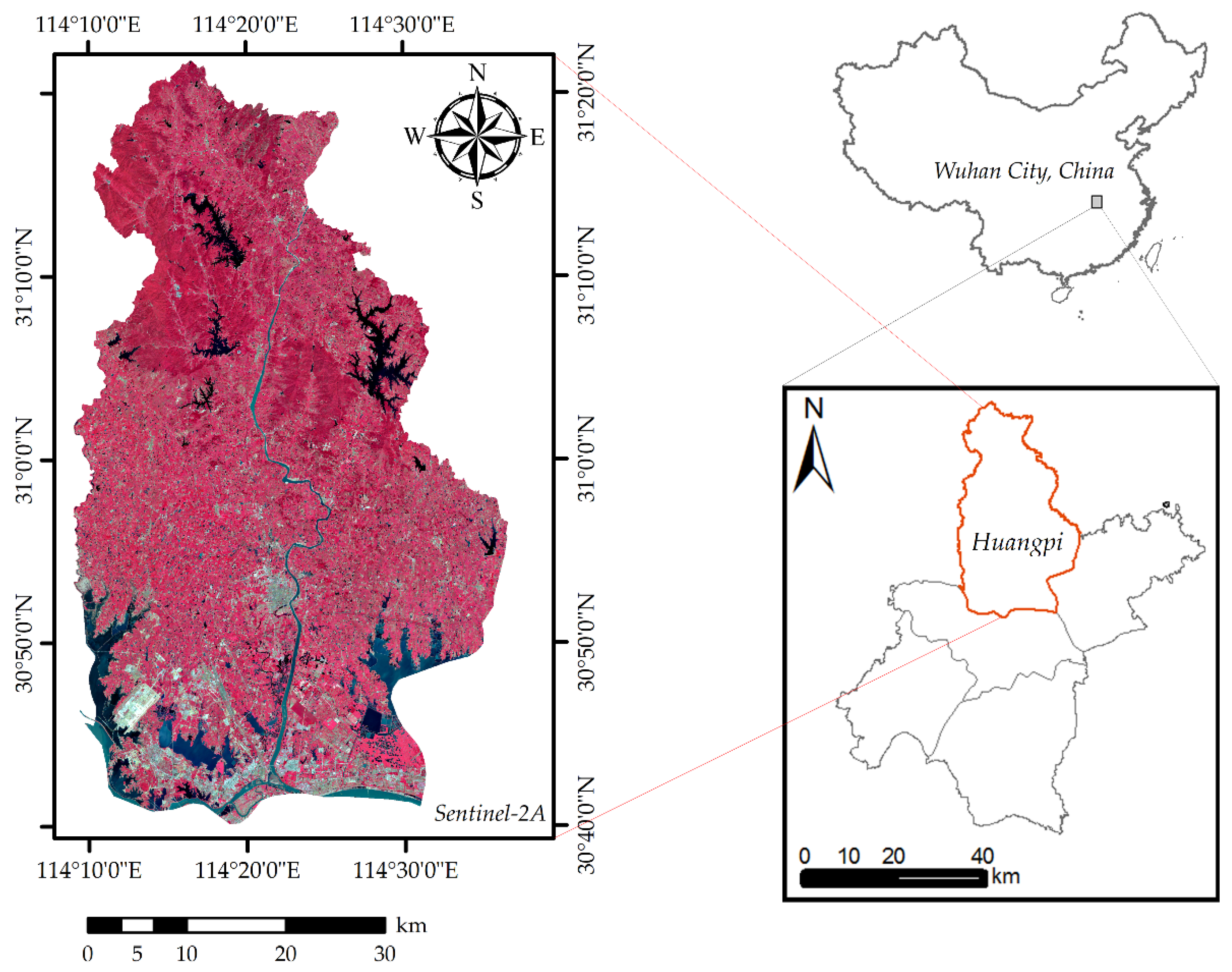
The study area illustrated in Figure 1, covering an area of 226,100 ha, is located in Wuhan, south-central China (30°37′–31°22′ N, 114°08′–114°37′ E, WGS84), where the terrain is a combination of the Jianghan plain and hills at an altitude between 16.5 and 850 m above sea level. The northern part of our study site includes the Dabie Mountains with an altitude between 150 and 850 m above sea level. The central part is the plain hillocks, with an elevation between 30 and 150 m. The south is a plain lake area with an altitude of fewer than 30 m. This study area belongs to the subtropical monsoon climate with abundant rainfall and sunlight. The average annual duration of sunlight is approximately 1917 h, and the average annual precipitation is about 1202 mm. This is an area in south-central China where precipitation is distributed throughout the year, rather than concentrated into one or more seasons. In this study area, the four single-dominant forest types are Chinese red pine (Pinus massoniana, L.), China fir (Cunninghamia lanceolata, L.), German oak (Quercus acutissima, Carruth) and Chinese white poplar (Populus lasiocarpa, Oliv), while the mixed forest types are mixed sclerophyllous broad-leaved forest, mixed soft broad-leaved forest, mixed broad-leaved forest and mixed coniferous forest [34,35], leading to the basis for classifying these forest types.
2.2. Data Acquisition and Preprocessing
The multi-spectral image data are elaborated in Section 2.2.1; the SAR data are described in Section 2.2.2; the DEM data derived from SRTM are introduced in Section 2.2.3; and a detailed explanation for the reference data is in Section 2.2.4.
2.2.1. Multi-Spectral Images
The Multi-Spectral Image (MSI) data used in this study are Sentinel-2A and Landsat-8 Operational Land Imager (OLI) images. A brief overview of our image datasets is listed in Table 1.
The Multispectral Sentinel-2A Images were collected by the Sentinel-2 satellite. This is a wide-swath, high-resolution, multi-spectral imaging mission, supporting land monitoring research; the data complement imagery from other missions, such as Landsat and SPOT imagery. The Sentinel-2 constellation includes two identical satellites (Sentinel-2A and Sentinel-2B). The Sentinel-2A satellite was launched on 23 June 2015 by the European Space Agency (ESA), while the Sentinel-2B launch was successfully completed in 2017. The revisit frequency of each satellite is 10 days, and the combined constellation revisit is five days. The Sentinel-2A satellite carries a state-of-the-art multispectral imager instrument with 13 spectral bands. Four bands have a spatial resolution of 10 m (blue: 490 nm, green: 560 nm, red: 665 nm and NIR: 842 nm); six bands have a spatial resolution of 20 m (red edge 1: 705 nm, red edge 2: 740 nm, red edge 3: 783 nm, narrow NIR: 865 nm, SWIR1: 1610 nm and SWIR2: 2190 nm); and three bands have a spatial resolution of 60 m (coastal aerosol: 443 nm, water vapor: 940 nm and SWIR_cirrus: 1375 nm). We used the Sentinel-2A bands with spatial resolutions of 10 m and 20 m in this study.
Two cloud-free Sentinel-2A MSI granules used in the study were freely acquired on 28 August and 7 September 2016 and downloaded from the Copernicus Scientific Data Hub (https://scihub.copernicus.eu/) as a Level-1C product. These two images contain three scenes and fourteen scenes, respectively, and details can be found in Table 2. The seventeen acquired Sentinel-2A images covered the study area and were collected in the leaf-on seasons, thus being conducive to forest type identification. We assume that there were no significant changes in the forested area during this period. The Level-1C product is composed of 100 × 100 km2 tiles (ortho-images in UTM/WGS84 projection). The Level-1C product results from using a Digital Elevation Model (DEM) to project the image in UTM projection and WGS84 geodetic system.
The Landsat-8 satellite was launched on 11 February 2013. Onboard are the operational land imager (OLI) and the thermal infrared sensor (TIRS), bringing new data and continuity to the Landsat program. The image produced by the OLI sensor is composed of nine spectral bands, of which eight bands have a spatial resolution of 30 m (coastal: 443 nm, blue: 485 nm, green: 563 nm, red: 655 nm, NIR: 865 nm, SWIR1: 1610 nm, SWIR2: 2200 nm and cirrus: 1375 nm). The system also provides a single, panchromatic band at a spatial resolution of 15 m. Only the first seven bands are used in our experiments. Table 2 shows the details of the nine images, including date acquired, the path and row and the percentage of cloud cover.
The nine Landsat-8 images listed in Table 3 were downloaded from the United States Geological Survey (USGS) Earth Explorer web (https://glovis.usgs.gov/) as a standard Level-1 topographic corrected (LT1) product with the UTM/WGS84 projection. The nine images belong to two different seasons (leaf-off and growing). Each season, we should collect three images to cover the whole study area. We assume that there were no significant changes for the ground features during different periods of the same season.
2.2.2. Synthetic Aperture Radar Data
The Sentinel-1 mission, a Synthetic Aperture Radar (SAR) satellite, is comprised of two polar-orbiting satellites (1A, 1B) with a 6-day repeat cycle, operating day and night performing C-band synthetic aperture radar imaging, enabling the system to acquire imagery regardless of the weather. Sentinel-1A was successfully launched by ESA in April 2014, and Sentinel-1B was launched in April 2016. It supports operation in single-polarization (HH or VV) and dual-polarization (HH + HV or VV + VH); the products are available in three models (SM, IW and EW) suitable for Level-0, Level-1 and Level-2 processing. The SAR data for our research are shown in Table 3.
As presented in Table 4, three Sentinel-1A IW Level-1 Single Look Complex (SLC) images, with a spatial resolution of 5 m by 20 m, were acquired on 22 and 27 August 2016 from the official website (https://scihub.copernicus.eu/). These images will be further processed and used to map the forest types.
2.2.3. SRTM One Arc-Second DEM
The Shuttle Radar Topography Mission (SRTM) is an international research effort that obtained digital elevation models on a near-global scale between 60° N and 56° S, with a specially modified radar system onboard the Space Shuttle Endeavour, collected during the 11-day STS-99 mission in February 2000. SRTM successfully gathered radar data for over 80% of the Earth’s surface with data points sampled at every one arc-second. The resulting Digital Elevation Model (DEM) was released under the name SRTM1 at a spatial resolution of 30 m; another version was released as SRTM3 at a 90-m resolution. These data are currently distributed free of charge by the USGS and available for downloading from the National Map Seamless Data Distribution System or the USGS FTP site. These data are provided in an effort to promote the use of geospatial science and applications for sustainable development and resource conservation. Five SRTM1 DEM images (n31e114, n30e115, n30e114, n30e113 and n29e114) covering our study area were acquired from the USGS Earth Explorer (http://earthexplorer.usgs.gov/), and used to extract topographic features, which can improve the results of forest type classification [11], especially when combined with spectral features [12,13].
2.2.4. Reference Data
To obtain reference data of pure and homogeneous stands of a forest type, a forest inventory map created in 2008 was used, which is a survey of forest resources and contains characteristics of dominant forest types, such as average height, Diameter at Breast Height (DBH), volume, age, canopy density, topographic factors and forest management type. The forest management type can be summarized as two types: one is commercial forest used for mainly developing economic benefit, and the other is ecological public welfare forest for green landscape and climate adjustment. In additional, most of the forest area in the study site is located in a biological reserve and belongs to the ecological public welfare forest, where the surface coverage is relatively difficult to change. The reference samples are manually outlined from the ecological public welfare forest type. Furthermore, in order to confirm whether the forestland type in the sample area has been changed, we also have a visual inspection of the high-resolution imagery of Google Earth in the same period. Thus, the used forest inventory data from 2008 have little negative influence on our results. The main forest types in the study area are four single-dominant forest types and four mixed forest types. Table 5 shows the details of the reference data (samples).
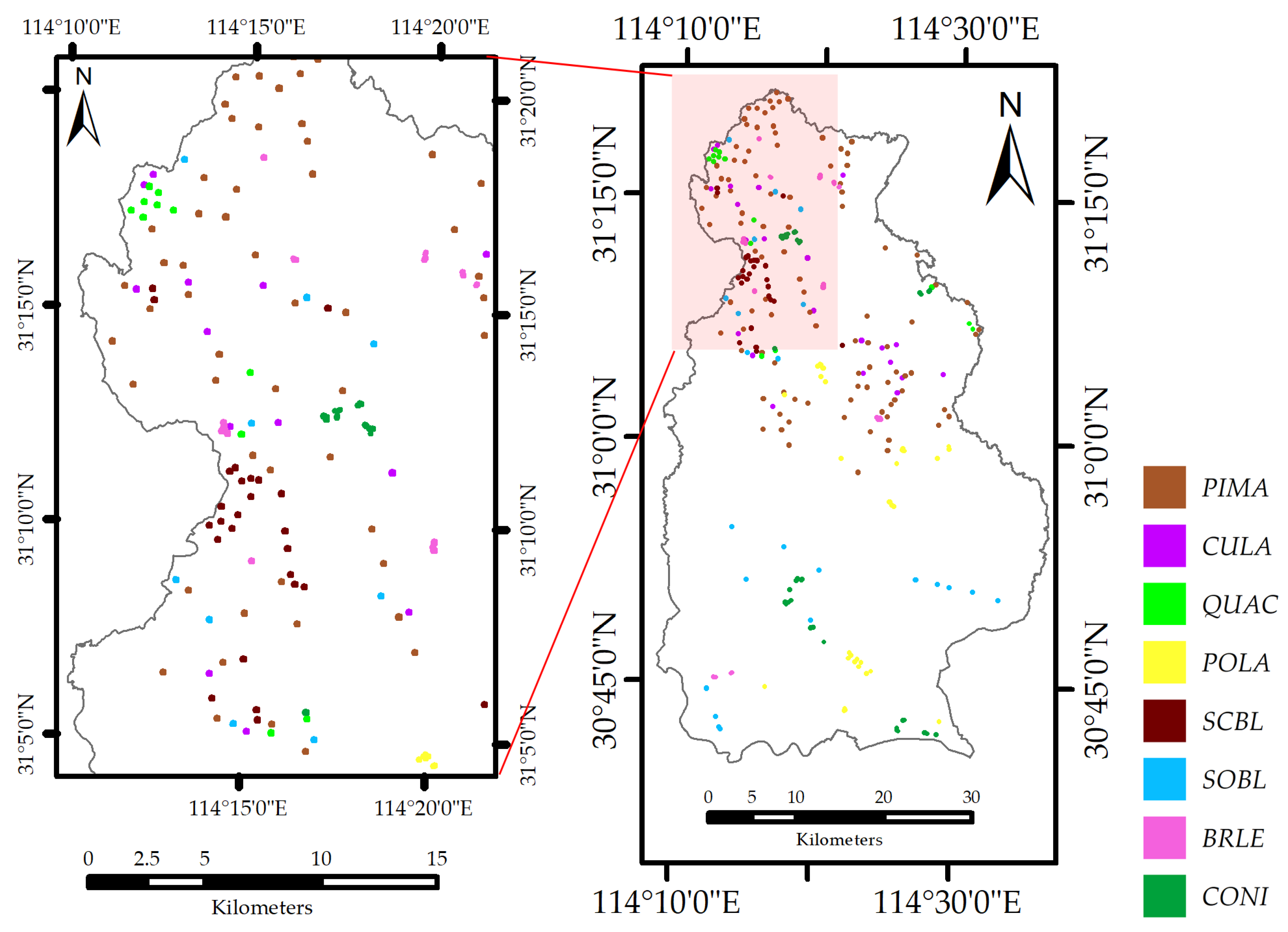
As can be seen from Table 5, two lines labeled as forest and non-forest (in the second column) describe the samples used for forest and non-forest classification, while the other eight lines record the samples used for classifying eight forest types. Considering that the mixed forest types may occur at the boundary of the plot acquired from forest inventory data and geometric correction error, we used a size of 9 × 9 pixels at the center of the plots as training and validation data. For the four single-dominant forest types, each polygon consists of an individual forest type. In the case of the four mixed forest types, each polygon consists of a group of adjacent forest types. As illustrated in Figure 2, the selected reference data were well distributed throughout the study site, and the forest categories of samples are Pinus massoniana (PIMA), Cunninghamia lanceolata (CULA), Quercus acutissima (QUAC), Populus lasiocarpa (POLA), Sclerophyllous Broad-Leaved (SCBL), Soft Broad-Leaved (SOBL), Broad-Leaved (BRLE) and Coniferous (CONI).
The reference data, shown in Figure 2, are manually outlined using the forest inventory map. In this study, we randomly and manually selected 3/4 of the sample data in each class evenly distributed in the study site as training data, while the rest for accuracy verification. The size of samples for each class varied from 25.11 ha–175.77 ha, and the size description of each class is listed in Table 5. The well-distributed samples and random selection strategy can be more robust and reliable for classification.
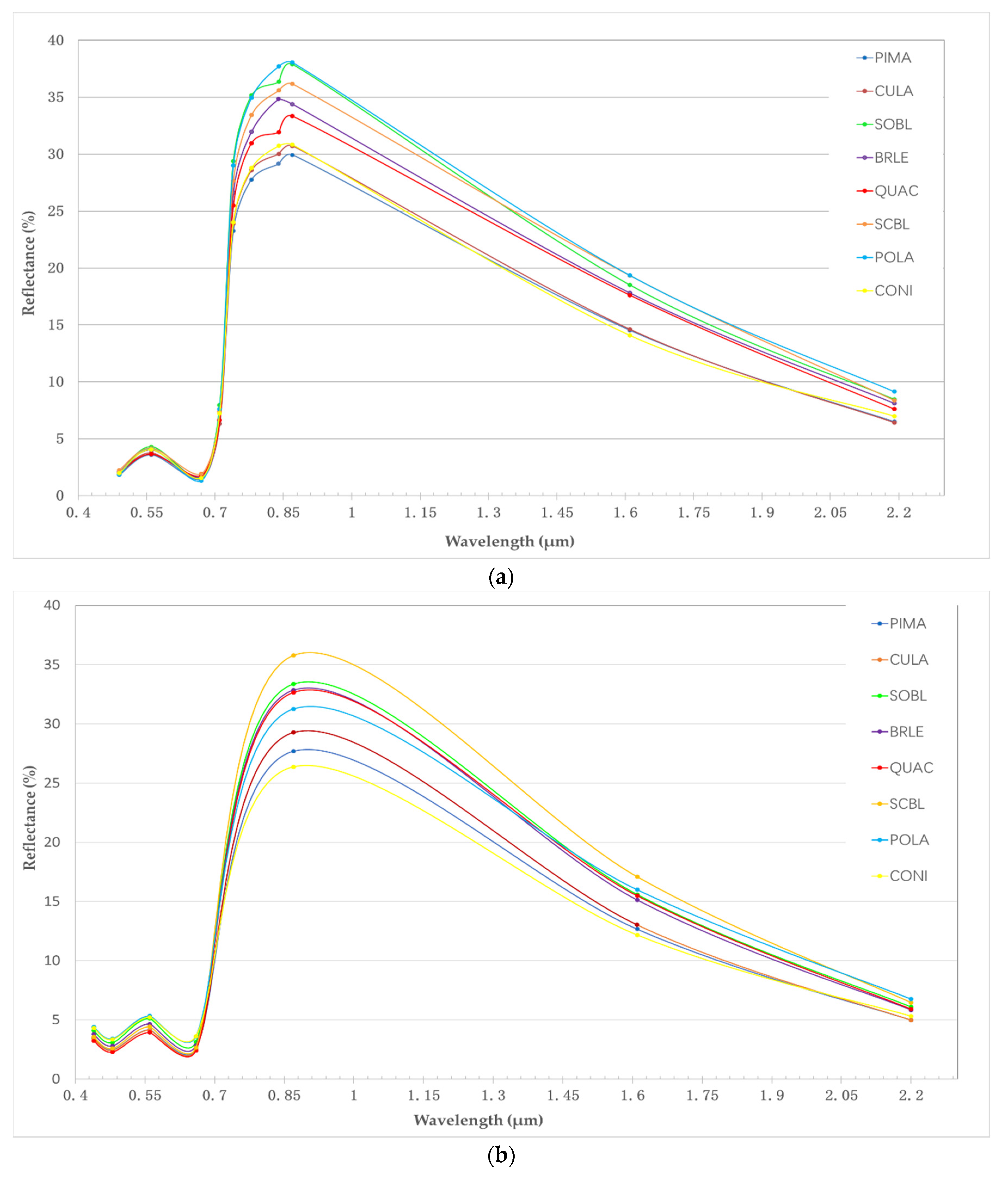
Figure 3 shows the mean spectral reflectance of the eight forest types within the delineated reference polygons on images of Sentinel-2A and Landsat-8. It can be seen that the spectral values of different forest types in Landsat-8 imagery vary more than the Sentinel-2A data in the visible light bands, but opposite in the SWIR bands. In addition, the forest type discrimination ability of Sentinel-2A images is better than Landsat-8 in the red-edge and near-infrared bands. What is more, the spectral values of Sentinel-2A and Landsat-8 imagery vary less in the visible light bands than the red-edge and near-infrared bands. Therefore, the red-edge and near-infrared bands are often regarded as the best bands to distinguish forest species. As expected, the spectral values of the broadleaf trees, such as POLA, SOBL, SCBL, BRLE and QUAC, are higher than the coniferous trees, such as CONI, CULA, and PIMA [36]. In addition, POLA has the highest spectral reflectance in the near-infrared band, while PIMA has the lowest in Figure 3a. SCBL has different spectral values in the near-infrared band. QUAC and BRLE are very similar in all seven bands in Figure 3b. However, the difference of spectral values between QUAC and BRLE is obvious in the near-infrared band of Sentinel-2A; thus, the configuration of Sentinel-2A and Landsat-8 images is conducive to forest type identification. The spectral reflectance of forest types gradually decreased in the red-edge and near-infrared bands and increased from late summer to high autumn in other bands [7,8]. Therefore, adding the phenology information can contribute to forest type identification.
3. Methods
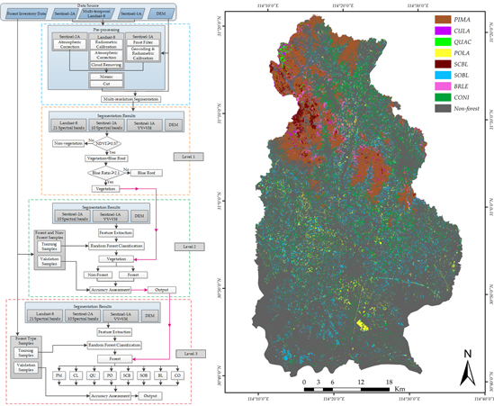
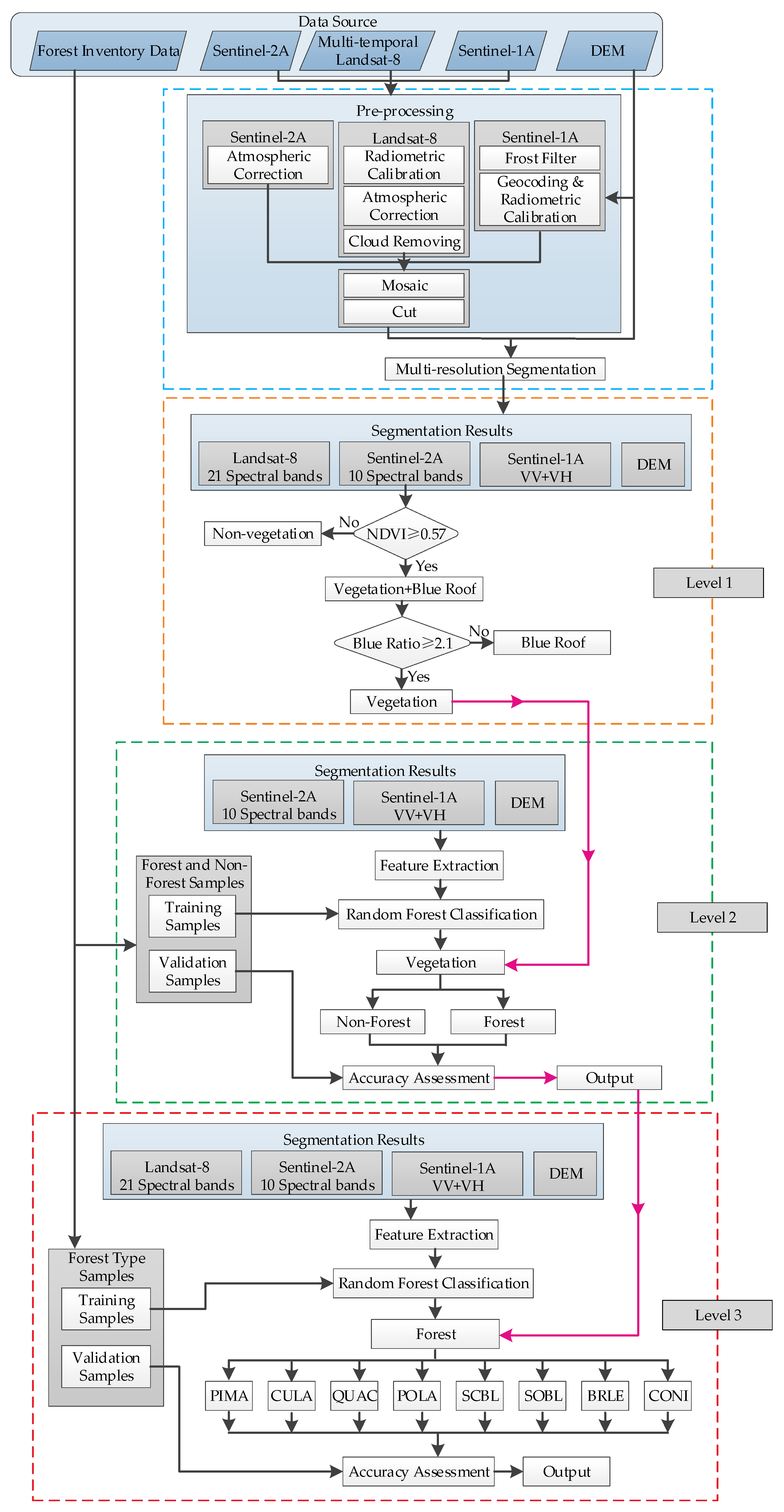
The proposed method, as illustrated in Figure 4, encompasses four key components, namely imagery segmentation, vegetation extraction, forested area extraction and forest type identification. Image preprocessing (Section 3.1) and multi-scale segmentation (Section 3.2) were applied to produce image objects. The object-based Random Forest (RF) approach (Section 3.3) was used for the hierarchical classification (Section 3.4). Threshold analysis based on NDVI and Ratio Blue Index (RBI) was used to extract vegetation at Level-1 classification (Section 3.4.1). Then, classification between forest and non-forest from the vegetation was finished at Level-2 classification (Section 3.4.2), and the identification of eight forest types was accomplished at Level-3 (Section 3.4.3). In the process of Level-2 and Level-3 classification, reference data were split into two parts for training and validation respectively, where 3/4 of sample data were randomly selected from each class as training data, while the rest for accuracy verification.
In this pipeline, operations in different stages are performed in sequence. A pre-processing and multi-scale segmentation are used for the multi-source images, generating the image objects as the basic input for the next operations. The vegetation is obtained in Level-1 by the NDVI and RBI threshold analysis. With the input vegetation, forested areas are extracted in the Level-2 state, and non-forest areas are removed. The map of forest types is accomplished in the Level-3 classification, producing eight dominant forest types.
3.1. Data Preprocessing
For the multispectral Sentinel-2A (S2) images, we performed atmospheric corrections with the SNAP 5.0 and Sen2Cor 2.12 software provided by the ESA. Two large scene Sentinel-2A images were mosaicked and then clipped, using the boundary of the study area. In this study, the bands with 60-m spatial resolution were not used, and other remaining bands with a spatial resolution of 10 m and 20 m were resampled to 10 m based on the nearest neighbor algorithm [37]. The downloaded Landsat-8 images were processed by ENVI 5.3.1 as follows: we performed radiometric calibration and atmospheric correction by the FLAASH atmospheric model, and the cloud cover was removed using a cloud mask, built from the quality assessment band in the Landsat-8. We applied a mosaicking process to these images and a clipped operation with the boundary of the study area. Moreover, Landsat-8 images were co-registered to the Sentinel-2A images and resampled at the spatial resolution of the first seven bands to 10 m by [37].
Sentinel-1A data were preprocessed in SARscape 5.2.1 using a frost filter to reduce the speckle noise. The backscatter values were radiometrically calibrated to eliminate terrain effects and georeferenced by converting the projection of the slant or ground distance to the geographic UTM/WGS84 coordinate system. To avoid the effects of small values, we transformed the result of calibration into a unit of dB as in:
where N is the per-pixel value calculated by geocoding and radiometric calibration. Sentinel-1A images were co-registered to the Sentinel-2A images and resampled to a 10-m resolution by [37], followed by a mosaicked process and clipped to the study area.
DNdB = 10·log10(N)
For the five SRTM1 DEM images in our study, the mosaicking and clipping operations on these images were firstly performed, then all DEM images were co-registered to the Sentinel-2A images and resampled to 10-m spatial resolution by [37]. The slope and aspect features are derived from the clipped DEM.
3.2. Image Segmentation by MRS
Image classification is based on the analysis of image objects obtained by Multi-Resolution Segmentation (MRS), which is known as a bottom-up region-merging technique. These objects are generated by merging neighboring pixels or small segmented objects. The principle of merging is to ensure that the average heterogeneity between neighboring pixels or objects is the smallest and the homogeneity among the internal pixels of the object is the greatest [38]. Our image segmentation is performed with the eCognition Developer 8.7. Four key parameters are used to adjust MRS: scale, the weight of color and shape, the weight of compactness and smoothness and the weights of input layers. The scale parameter is used to determine the size of the final image object, which corresponds to the allowed maximum heterogeneity when generating image objects [39,40]. The larger the scale parameter, the larger the size of the generated object, and vice versa. Homogeneity is used to represent the minimum heterogeneity and consists of two parts, namely color (spectrum) and shape. The sum of the weights for the color and shape is 1.0. The weights of color and shape can be set according to the characteristics of land cover types in the images. The shape is composed of smoothness and compactness. The former refers to the degree of smoothness for the edge of the segmented object, and the later refers to the degree of closeness of the entire object. The sum of the weights for the smoothness and compactness is also 1.0. The weights of input layers are used to set the weight of the band to participate in the segmentation. We can set the weights of input layers according to the requirements of the application.
In this study, the four 10-m resolution bands (Band 2, 3, 4, and 8) of Sentinel-2A were used as the MRS input layer to define objects, and a similar operation was applied to other images using the segmented boundary. An analysis of MRS was performed by different segmentation parameter sets, and visual assessment was done based on comparing the matching between the segmented objects and the reference polygons for the segmented results using the trial and error approach [17], selecting 30, 0.1 and 0.5, for the scale, shape and compactness parameters, respectively.
3.3. Object-Based Random Forest
To handle a large number of input variables and the limited sample data, our classification in stages at Level-2 and Level-3 was accomplished by an object-based classification method: Random Forest (RF) [31]. RF is an integrated learning method based on a decision tree, which is combined with many ensemble regression or classification trees [29] and uses a bagging or bootstrap algorithm to build a large number of different training subsets [41,42]. Each decision tree gives a classification result for the samples not chosen as training samples. The decision tree “votes” for that class, and the final class is determined by the largest number of votes [24]. This approach can handle thousands of input variables without variable deletion and is not susceptible to over-fitting as the anti-noising ability is enhanced by randomization. The weight of the variables as feature importance can be estimated [42].
To estimate the importance in forest construction, internal unbiased error estimation uses Out-Of-Bag (OOB) sampling, in which objects from the training set are left out of the bootstrap samples and not used to construct the decision trees. There are two ways to calculate variable importance: the Gini coefficient method and the permutation variable importance approach [31]. The former is based on the principle of impurity reduction, while the latter, selected in our RF analysis, is based on random selection and index reordering. The permutation variable importance method was carried out to measure variable important. First of all, the accuracy of prediction in the OOB observations are calculated after growing a tree, then the accuracy of prediction is computed after the association between the variable of interest, and the corresponding output is destroyed by permuting the values of all individuals for the variable of interest. The importance of the variable of interest from a single tree is calculated by subtraction of the two accuracy values. The final importance for the variable of interest is obtained by calculating the average value of all tree importance values in random forest. The same procedure is carried out for all other variables.
In this study, the random forest approach including the estimation of OOB was programmed with OpenCV2.4.10. Three parameters must be set: the number of decision trees (NTree), the number of variables for each node (SubVar) and the maximum depth of a tree (MaxDepth). We set NTree to 20, MaxDepth to 6 and SubVar to one-quarter of the total number of input variables for all tested scenarios.
3.4. Object-Based Hierarchical Classification
The forest type mapping was obtained through a hierarchical strategy, including vegetation classification at the first level, forestland extraction at the second layer and forest type classification at the third level.
3.4.1. Vegetation Classification at Level-1
The first level of classification is to extract vegetation from land cover and contains two steps. The first step is vegetation and blue roof extraction using the Normalized Difference Vegetation Index (NDVI) threshold analysis and then removal of blue roofs misclassified as vegetation by the Ratio Blue Index (RBI) threshold analysis. NDVI has been ubiquitously used for vegetation extraction in global land processes [43,44]. In this study, it was calculated from near-infrared and red bands using the 10-m spatial resolution of Sentinel-2A, written as:
where and are the reflectance from the near-infrared and red bands, respectively.
The NDVI threshold analysis is performed by the stepwise approximation method [20]. The principle of this method is first to fix an initial threshold in the NDVI histogram and then determine the optimal threshold when the image objects of vegetation are best matched by visual inspection. However, there exists an overlap in NDVI values between blue building roofs and vegetation, which means that some blue roofs can be misclassified as vegetation. Compared to the vegetation, the mean reflection value of the blue roof is higher in the visible light bands, while being lower in the near-infrared band [45]. To distinguish blue roofs and vegetation, a Ratio Blue Index (RBI) threshold analysis based on the stepwise approximation is further carried out, consistent with the process of vegetation extraction. RBI is the band ratio of the near-infrared to blue roofs, defined by:
where and are the reflectance of the near-infrared and blue bands, respectively. In this study, we set the threshold of NDVI to 0.57 for non-vegetation removal, and RBI is 2.1 for blue roof removal, leading the pure vegetation to further classification at Level-2.
3.4.2. Forestland Classification at Level-2
The second hierarchical (Level-2) classification is to extract forest and non-forest objects from the acquired vegetation at Level-1 using the RF approach. RF classification was carried out to evaluate the relative contributions of S2, S1, DEM and L8 on forestry land extraction by four experiments. To accomplish this process, texture features, spectral features and topographic features were firstly extracted from the segmented objects. The spectral features are comprised of land cover surface reflectance and vegetation indices acquired from the combination of visible and near-infrared spectral bands, as well as a simple, effective and empirical measure of surface vegetation conditions. Texture features are calculated by texture filters based on co-occurrence matrix. This matrix is a function of both the angular relationship and distance between two neighboring pixels and shows the number of occurrences of the relationship between a pixel and its specified neighbor [46,47]. These filters include mean, variance, homogeneity, contrast, dissimilarity, entropy, second moment and correlation. To reduce high dimensional and redundant texture features, Principal Component Analysis (PCA) is carried out to achieve a more accurate classification result by [48]. As shown in Table 6, a total of 36 features derived from Sentinel-2A and DEM imagery was chosen to extract the forested areas, including 21 spectral features, 12 textural features and three topographic features.
As presented in Table 6, the spectral features include the mean value of each band for Sentinel-2A and vegetation indices. In this study, we extract the texture features using the 10-m spatial resolution bands of the Sentinel-2A images (Sb2, Sb3, Sb4 and Sb8) and obtain three principal components based on PCA, which can explain 95.02% of our texture features. Topographic features are represented by a DEM, aspect and slope, and the features of aspect and slope are extracted from the DEM. RF begins with these 36 features acquired from the S2 and DEM imagery and outputs the forested areas as input for the Level-3 classification.
3.4.3. Forest Type Classification at Level-3
The main object of Level-3 classification is to classify forested area into more detailed forest types, which are combined with the four single-dominant forests and the four mixed forest types, according to the actual distribution in our study area. Among these species, CONI can be more easily distinguished than the other three mixed forest types due to the significant spectral differences between them. For the type of coniferous (e.g., PIMA and CULA) or the mixed-broadleaf forest (e.g., QUAC and POLA), it is more difficult to identify these species from a single dataset due to the high similarity between spectrums. Therefore, other features such as topographic and phenology information must be collected to improve classification results. In this study, a multi-source dataset (S1, S2, DEM and L8) was obtained from four kinds of sensors. As shown in Table 7, the 59 features derived from these multi-source images, including 21 spectral features from S2, three topographic features derived from DEM, two backscattering features obtained from S1 and 33 spectral features from L8 time-series images, were used to find the best configuration for classifying eight forest types.
As shown in Table 7, the 21 spectral features extracted from S2 images are consist with the average spectral values of each band and vegetation indexes, which are a combination of visible and near-infrared bands, like the Normalized Difference Vegetation Index (NDVI), Ratio Vegetation Index (RVI), Enhanced Vegetation Index (EVI) and Difference Vegetation Index (DVI). The three topographic features are DEM, aspect and slope; in particular, aspect and slope are calculated from the DEM. The two backscattering features (VV, VH) obtained from Sentinel-1A are also used in forest type mapping. The 33 spectral features derived from the multi-temporal L8 images are chosen to capture temporal information, indicating physiological growth and phonological changes. Forest type identification was accomplished by RF using the combination of these features, and the accuracy was significantly improved with the added temporal information from L8 imagery.
4. Results
4.1. Results of Forest Type Mapping
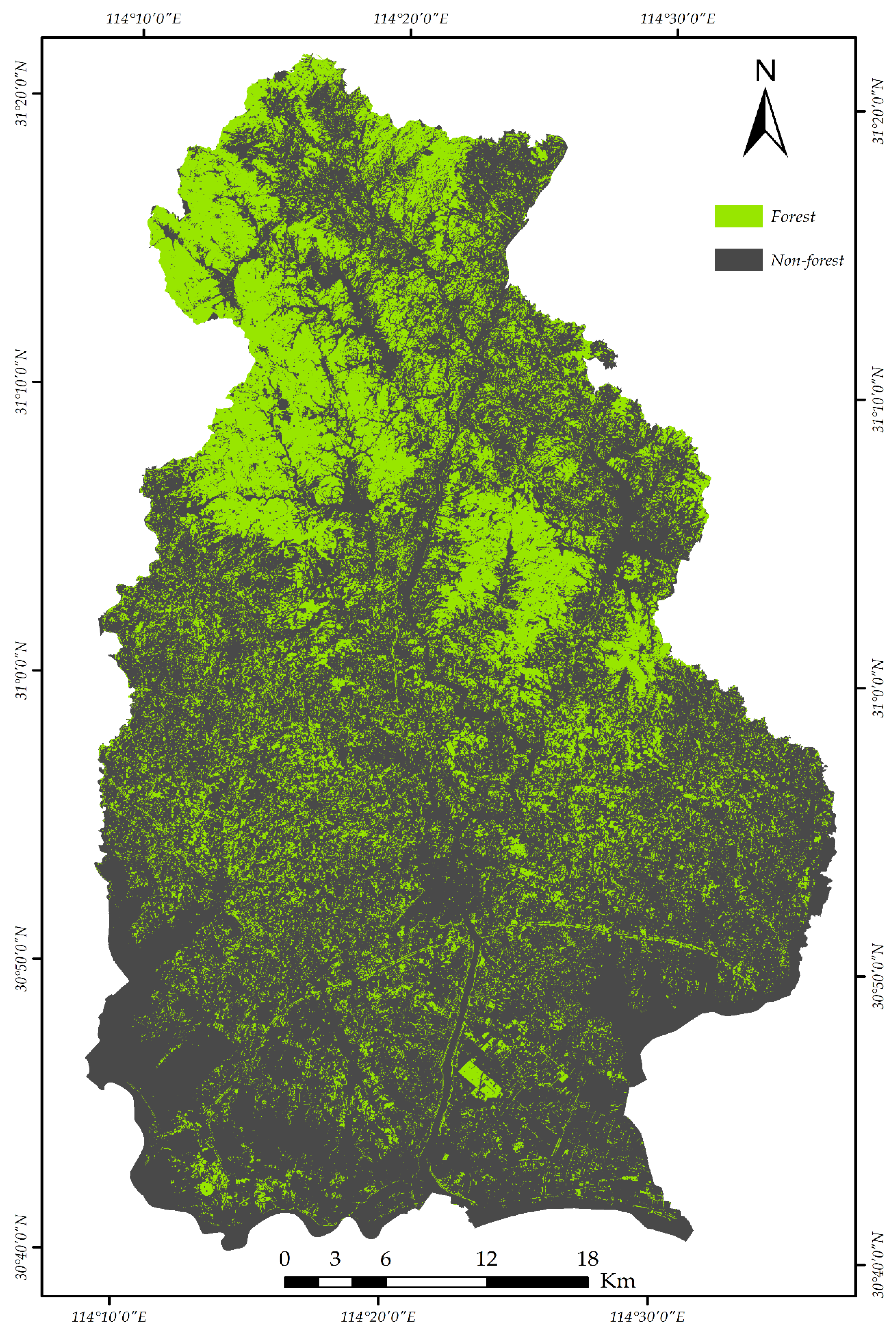
The forestland (Level-2 classification) was extracted based on RF by the best combination of Sentinel-2A and DEM images with an overall accuracy of 99.3% and a kappa coefficient of 0.99, respectively. As shown in Figure 5, the forest was colored with green, and non-forest was colored with black.
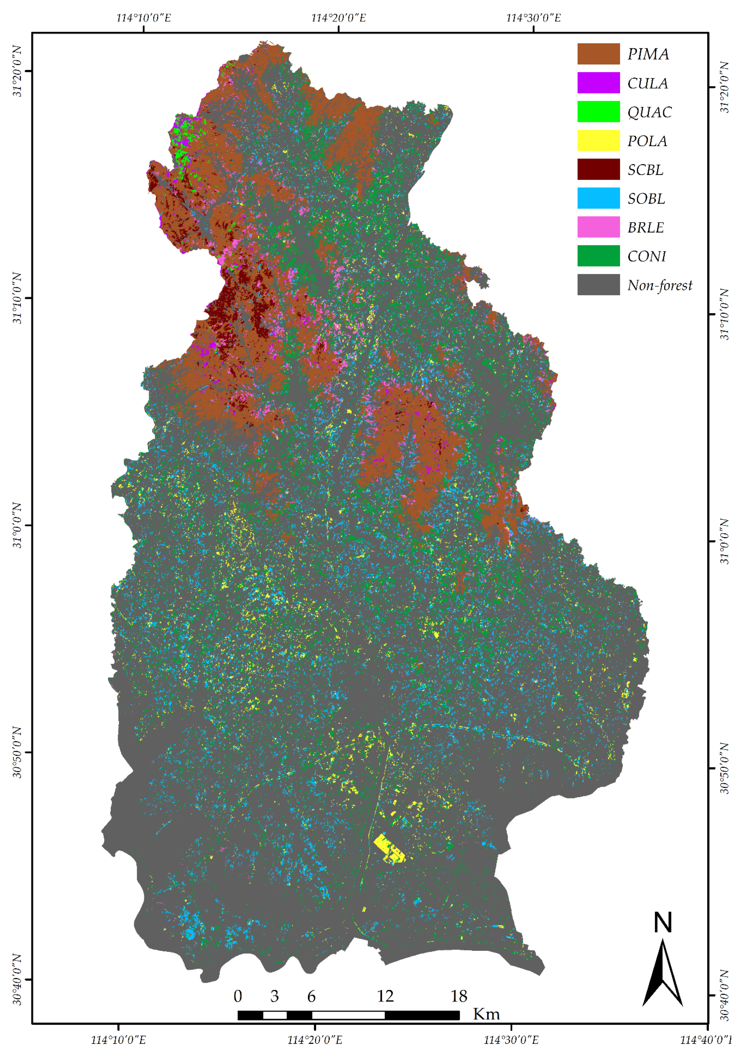
The final mapping of the eight forest types is shown in Figure 6, and corresponded to the actual distribution of forest types [21,49].
As can be seen from Figure 6, PIMA was the most abundant dominant forest type located on ridges and near the Mulanshan National Park, Wuhan. The proportion of CULA and QUAC was relatively small, concentrated in the east of the Mulanshan National Park. Woodland was found in the mountainous areas in the northern part of the study site, while the coniferous forests were the most ubiquitously distributed forest species, according to forest inventory data and reports from the website of the Forestry Department [34]. Furthermore, the QUAC stands were mainly distributed on the ridge and south-facing side of the slope, which was in line with the favorable habitat for QUAC. For POLA, although the amount was not large, it was scattered in the south and center parts of the study area, and more isolated than other forest types. The spatial distribution of heterogeneous mixed forest such as the SOBL and CONI forest types was more likely to be located on the low-elevation slopes and flat areas near communities. On the other hand, SCBL and BRLE had smaller areas compared to SOBL and CONI, concentrating in the lower altitude mountainous areas. The distribution of SOBL, POLA and SCBL seemed reasonable, and the accuracy of classification was much higher.
However, there were still some biases from the mapping results, revealed by the visual inspection. The tree crowns classified as BRLE yielded lower classification accuracy because of some mixed broad-leaved forest in the northwest were, in reality, mixed stands with PIMA and CONI, while BRLE was more likely to be found around water bodies. This is consistent with mixed forest habitats, which there are more likely to grow in a place with cool and rich soil with shade. CULA was under-represented, and PIMA was overrepresented due to the similarity of spectral features. In addition, QUAC was underrepresented due to confusion with SCBL and PIMA, while the amount of CONI might have been a little high as some PIMA may have been misclassified as CONI. The overall accuracy of the mapping results of the forest types in the study area was approximately 82.12%, with the highest amount of PIMA and CONI, consistent with [34,35]. Detailed assessments and analysis of the hierarchical classification by RF including the weights of features will be given later.
4.2. Feature Importance of Forest Type Identification
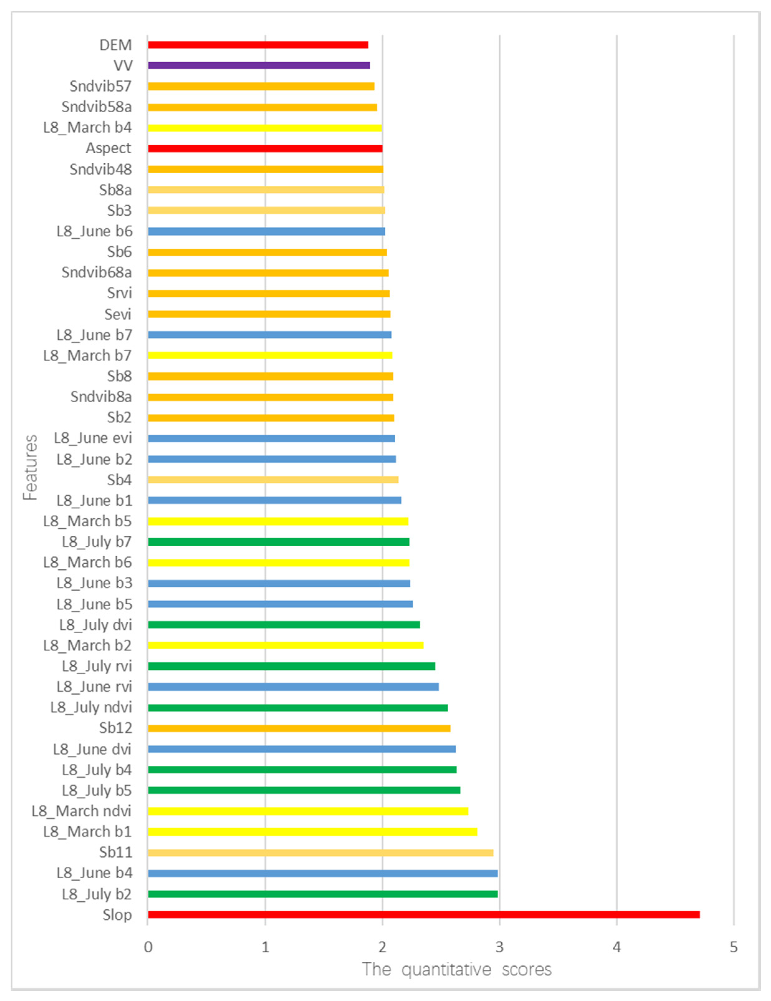
The importance of features (feature importance) can be used to extract the implicit importance of the used feature attributes at Level-3 classification with the substitution method and were calculated by analyzing the split samples of a random forest model. The features with higher weight were considered more relevant and important. We have evaluated and analyzed the feature weights to benefit from all features from the final forest type mapping. Figure 7 illustrates the feature importance of forest type identification with the highest accuracy, where the colored bars are the feature importance of the forest, along with their inter-tree variability. The higher the quantification value of a feature, the more important is the feature.
Figure 7 displays the importance of 43 features (described in Table 6 in Section 3.4.3), which were selected by RF for forest type identification, including three topographic features, one backscattering feature (VV) and 39 spectral features. These features were acquired from the highest accuracy at the Level-3 classification using S1, S2, DEM and L8 images, and the importance of features was assessed by the substitution method of RF. The most pivotal feature was the slope, a topographic feature extracted from DEM, indicating that the feature of the slope contributed the most to forest type identification, especially in mountain areas. Phenological features (e.g., L8_July b2, L8_June b4, Sb11, L8_March b1, L8_March ndvi, L8_July b5, L8_July b4, L8_June dvi, Sb12, L8_July ndvi, L8_June rvi, L8_July rvi, L8_March b2) extracted from Landsat-8 in March, June and July and Sentinel-2A in late August and early September were the next most pivotal as these features representing phenology information obtained consistently higher quantization scores. Although the contribution of some features was relatively low, such as the backscattering features obtained from VV images of Sentinel-1A, they were still helpful in terms of improving the accuracy of classification. This is because the microwave from the Sentinel-1A penetrates into forests interacting with different parts of trees, producing big volume scattering.
4.3. Accuracy Assessment for Forest Types
Table 8 summarizes the results of four classification scenarios for forestland extraction, where the highest accuracy (99.30%) was achieved by the combined Sentinel-2A and DEM images.
To classify eight types of forest further, seven classification scenarios were compared to obtain the most suitable combination of the multi-source dataset. The classification schemes are presented in Table 9, where the remote sensing imagery, the overall accuracy and the kappa coefficient are listed for each tested scenario.
The scenarios summarized in Table 9 indicate that the use of different image combinations can facilitate forest type identification. The overall accuracy of classification ranged from 50.00–82.78% with kappa coefficients between 0.38 and 0.78. As can been seen from Table 9, forest type identification using only Sentinel-2A imagery produces higher overall accuracies (54.31%, Scenario 1) than using only Landsat-8 data acquired in July (50.0%, Scenario 2). This is because there are three red-edge bands and two near-infrared bands for Sentinel-2A imagery, which are conducive to forest type identification based on the spectral feature curve in Figure 3. In addition, the spatial resolution of Landsat-8 imagery is lower than the Sentinel-2A imagery, and the larger pixels imply a greater spectral mixture of classes [50]. Therefore, in the following experiment, we used Sentinel-2A data as the basis, then gradually added the multi-temporal Landsat-8, DEM and Sentinel-1 imagery for a further comparative analysis. Compared with the forest type identification using only Sentinel-2A imagery (54.31%, Scenario 1), the overall accuracy was improved by about 15.23% when combining DEM and Sentinel-2A data (69.54%, Scenario 3). This result illustrated that the spatial distribution of different forest types is greatly affected by topographic information. Additionally, the overall accuracy was greatly improved by about 22.51% when combining multi-temporal Landsat-8 and Sentinel-2A imagery (76.82%, Scenario 7). Therefore, we concluded that phenology information is very important for forest type identification. In Scenario 4, we used the fused Sentinel-2A, DEM and multi-temporal Landsat-8 imagery to map forest types and obtained an overall accuracy of 80.13%. Moreover, the highest overall accuracy was obtained from Scenario 5 by the continuously added VH polarized images. However, the overall accuracy was not well improved when adding Sentinel-1 data in Scenario 6. We obtained the best combination of multi-source imagery from the Scenario 5, where the result illustrated that multi-source remotely sensed data have great potential for forest type identification by complementary advantages with spatial resolution, temporal resolution, spectral resolution and backscattering characteristics, leading to a more favorable recognition environment to identify forest types.
A further accuracy assessment for the classification of Scenario 5 is summarized by a confusion matrix. A quarter of the reference data were chosen to validate the classification accuracy. These selected samples, with an average size of 9 × 9 pixels, were distributed among the actual forest types. Table 10 shows the detailed evaluation on the most suitable configuration of forest type mapping, including the user’s and producer’s accuracy, the overall accuracy and the kappa coefficient.
From the assessment of the confusion matrix in Table 10, each of the four single-dominant species (PIMA, CULA, QUAC and POLA) and the four mixed forest species (SCBL, SOBL, BRLE and CONI) contained at least one misclassification. The producer accuracies of per-class varied from 50–96.30%, and the user accuracies ranged from 68.75–100%, respectively. In addition, CONI and POLA showed more than 80% producer’s and user’s accuracies, which means that we have obtained small omission and commission errors, achieving the best classification results. For the four mixed forest types, SOBL obtained the smallest producer accuracy (71.43%), and therefore, it represented the highest omission error among all the mixed forest types. SCBL, CONI and SOBL each have achieved more than 80% user’s accuracy, while BRLE obtained the smallest with 68.75%. CONI has obtained the highest producer’s accuracy of 93.75% in the four mixed forest types. For the four single-dominant species, the classification of PIMA and POLA resulted in a producer’s accuracy of more than 90%, representing a small omission error. However, for the CULA and QUAC, the producer’s accuracies were 58.33% and 50%, respectively. CULA, BRLE and SOBL were mistakenly classified as PIMA, and as a result, PIMA represented the smallest user accuracy (78.79%), followed by CULA with 87.50% accuracy. QUAC obtained the highest user accuracy of 100%, which demonstrated that there was no misclassification.
Furthermore, we observed that the mixed forest types obtained the greatest confusion error compared to the single-dominant types, especially BRLE and CONI. For the four single-dominant species, misclassification between the same forest type (e.g., CULA and PIMA from conifers, POLA and QUAC from broadleaf) occurred at a higher rate than it did between different types, as conifers and broadleaf [51]. The bidirectional reflectance is not only related to the reflection characteristics of the land cover, but also to the radiation environment, which may explain why the PIMA class was misclassified as SCBL. Moreover, the changes in reflectance for the same land cover forest area, caused by the sun angle and slope at a different time, will bring some incorrect classification. Some forest types are highly heterogeneous in terms of landscape, and there is no obvious boundary between them. For example, both BRLE and SCBL are mixed forest types and difficult to identify during on-site acquisition, increasing the difficulty of classification. One of the most pivotal results of the confusion matrix from the highest accuracy in forest type identification was that a large number of zeros indicated that the proposed forest type identification method had achieved a great deal of success [52].
5. Discussion
This study demonstrates that freely-accessible multi-source imagery (Sentinel-1A, Sentinel-2A, DEM and multi-temporal Landsat-8) could significantly improve the overall accuracy of forest type identification by comparative analysis of multiple scenario experiments. We obtained a more accurate mapping result of forest type than the previous studies using Sentinel-2A or similar free satellite images. Immizer et al. [17] mapped forest types using Sentinel-2A data based on the object-oriented RF algorithm in Central Europe with an overall accuracy of 66.2%. Dorren et al. [13] combined Landsat TM and DEM images to identify forest types in the Montafon by an MLC classifier and obtained an overall accuracy of 73%. In addition, the number of identified forest types in this study, especially the mixed forest types, was more than previous studies [17,20]. Compared with the Landsat-8 imagery in Scenario 2, the overall accuracy can be improved by 4.31% when using only the Sentinel-2A imagery, which means that the Sentinel-2A imagery was more helpful to map forest types. The slop feature (Figure 7) derived from the DEM data contributed the most to classifying forest types, indicating that the spatial distribution of forest types is greatly influenced by topographic information. In addition, the Sentinel-1A images also have a contribution to the classification accuracy with an approximately 2.65% improvement (Scenario 5 in Table 9).
Regarding the employed multi-source imagery, these data consistently improved the overall accuracy of forest type identification. The time-series Landsat-8 and Sentinel-2A data, covering the crucial growing and leaf-off seasons of the forest, could provide phenological information to improve the discrimination between different forest types. This result is in good agreement with the findings of [19,50], who summarized that time-series images can obtain much higher accuracy of mapping tropical forest types. Macander et al. [53] have also used seasonal composite Landsat imagery and the random forest method for plant type cover mapping and found that multi-temporal imagery improved cover classification. Topographic information derived from the DEM can better offer different geomorphologic characteristics. These characteristics reflect the habitats of different forest types and can help to identify forest types, similar to the studies established by [13,50]. Seen from the experimental results of forest type identification by using only Landsat-8 and Sentinel-2A imagery, we concluded that Sentinel-2A images can achieve a higher overall accuracy due to its high spatial resolution (Table 9 and Table 10). This result is the same as [50], who concluded that the classification using Sentinel-2 images performed better than Landsat-8 data.
Regarding the strategy of hierarchical classification based on object-oriented RF, it can better and more flexibly combine data from multiple sources and simplify the complex classification problem into a number of simpler classifications. Zhu et al. [19] successfully mapped forest types based on two-level hierarchical classification using dense seasonal Landsat time-series images in Vinton County, Ohio. In our study, three-level hierarchical classification was carried out to map forest types. First, we extracted vegetation from land-cover utilizing two threshold analyses based on NDVI and RBI. Owing to RVI threshold analysis, we can well remove blue roofs misclassified as vegetation; because RVI improves the discrimination between forest types based on the different spectral characteristics in blue and near-infrared bands. For the second-level classification, Sentinel-2A and DEM images are enough to identify forestland and non-forest land. In the third-level classification, we fused information from images of DEM, time-series L8, S2 and S1 to better use the forest type structure habits and phenology. If we do not use hierarchical classification, combining all multi-source data to identify all classes will be time consuming. In addition, we can tune the parameters of RF separately to obtain optimal results from each classification level using the strategy of hierarchical classification. For the hierarchical approach, the RF classifier can assess the importance of features for the class of interest rather than all classes.
Regarding the classification algorithm and classifier performance, it was observed that the object-based Random Forest (RF) method was incredibly helpful to identify forest types in our tested scenarios. In the process of hierarchical classification, RF uses a subset of features to build each individual hierarchy, making a more accurate classification decision based on effective features and reducing the error associated with the structural risk of the entire feature vector. Novack et al. [54] showed that RF classifier can evaluate each attribute internally; thus, it is less sensitive to the increase of variables (Table 5 and Table 6). The object-based classifier can provide faster and better results and can be easily applied to classify forest types [24,39,40,55]. In addition, this classification method has the ability to handle predictor variables with a multimodal distribution well due to the high variability in time and space [50,56]; especially, no sophisticated parameter tuning is required. Thus, it could obtain a higher overall accuracy.
Regarding the feature importance for the highest accuracy of forest type classification (Figure 7), the input features were evaluated by the substitution method [33], and the feature distribution from the highest classification accuracy of forest types is consistent with some previous studies [51,57,58]. The slope and phenological features with higher quantization scores were the two most pivotal features for forest type identification. The classification accuracy listed in Table 8 was significantly improved by combining phenology information from multi-temporal L8 images and Sentinel-2A imagery, and the overall accuracy was raised at least 22.51% (Scenario 7); this result is in line with the research of [18,53], who reported that the multi-temporal imagery was more effective for plant type cover identification. The feature vegetation index in the bands of red and near-infrared from the Sentinel-2A also contributes to forest type classification, and other features abstracted from Sentinel-2A, DEM and multi-temporal Landsat-8 images (e.g., L8_June b6, L8_March b4, etc.) are listed as important. The removal of any feature can lead to a reduction in the overall accuracy, emphasizing the importance of topographic and phenology information for forest type identification. In addition, the backscattering features obtained from VV images of Sentinel-1A had a nearly 2.65% improvement for forest type classification between Scenario 4 and 5 (Table 8), which demonstrates that VV polarization radar images can help to improve classification accuracy, while using VV and VH features from Sentinel-1 data in Scenario 6 (Table 8) was less successful as the overall accuracy decreased by 1.32% compared to Scenario 5, which means that VV polarization imagery was found to better discriminate forest types than VH polarization data. The quantitative scores of features described in Figure 7 indicate that the 43 features extracted from the multi-source remote sensing data can be applied to map the forest types.
This study suggests that freely-available multiple-source remotely-sensed data have the potential of forest type identification and offer a new choice to support monitoring and management of forest ecological resources without the need for commercial satellite imagery. Experimental results for eight forest types show that the proposed method achieves high classification accuracy. However, there still was misclassification between the forest types with similar spectral characteristics during a phonological period. As can be seen from the assessment report in Table 9, the incorrect classification between BRLE and PIMA, CULA and PIMA was always caused by the exceedingly high spectral similarity, especially in the old growth forests where shadowing, tree health and bidirectional reflectance exist [51,59]. Hence, some future improvements will include obtaining more accurate phenological information from Sentinel-2 and using 3D data like the free laser scanning data [60,61,62,63]. In general, the proposed method has the potential for mapping forest types due to the zero cost of all required remotely-sensed data.
6. Conclusions
In this study, we used freely-accessible multi-source remotely-sensed images to classify eight forest types in Wuhan, China. A hierarchical classification approach based on the object-oriented RF algorithm was conducted to identify forest types using the Sentinel-1A, Sentinel-2A, DEM and multi-temporal Landsat-8 images. The eight forest types are four single-dominant forest (PIMA, CULA, QUAC and POLA) and four mixed forest types (SCBL, SOBL, BRLE and CONI), and the samples of forest types were manually delineated using forest inventory data. To improve the discrimination between different forest types, phenological information and topographic information were used in the hierarchical classification. The final forest type map was obtained through a hierarchical strategy and achieved an overall accuracy of 82.78%, demonstrating that the configuration of multiple sources of remotely-sensed data has the potential to map forest types at regional or global scales.
Although the spatial resolution of the multispectral images is not exceedingly high, the increased spectral resolution can make up for the deficiency of the spatial resolution, especially for Sentinel-2A images. The most satisfying results obtained from the combination of multi-source images are comparable to previous studies using high-spatial resolution images [64,65]. These free multiple-source remotely-sensed images (Sentinel-2A, DEM, Landsat-8 and Sentinel-1A) provide a feasible alternative to forest type identification. Given the limited availability of Sentinel-2A data for this study, the multi-temporal Landsat-8 data were used to extract phenology information. In the future, the two twin Sentinel-2 satellites will provide free and dense time-series images with a five-day global revisit cycle, which offers the greatest potential for further improvement in the forest type identification. In general, the configuration of Sentinel-2A, DEM, Landsat-8 and Sentinel-1A has the potential to identify forest types on a regional or global scale.
Author Contributions
Conceptualization, Y.L., W.G., X.H. and J.G. Methodology, Y.L., X.H. and J.G. Software, Y.L. Resources, X.H. and J.G. Writing, original draft preparation, Y.L., W.G. Writing, review and editing, Y.L., W.G., X.H. and J.G. Visualization, Y.L. and W.G. Supervision, X.H. and J.G. Project administration, Y.L., W.G., X.H. and J.G. Funding acquisition, X.H. and J.G.
Funding
This work was jointly supported by the National Key Research and Development Program of China, Grant Numbers 2017YFB0503700, 2016YFB0501403; the Grand Special of High Resolution on Earth Observation: Application demonstration system of high-resolution remote sensing and transportation, Grant Number 07-Y30B10-9001-14/16.
Acknowledgments
We would first like to thank the anonymous reviewers, and we thank Stephen C. McClure for his kind help to improve the language.
Conflicts of Interest
The authors declare no conflict of interest.
References
- Reay, D.S. Climate change for the masses. Nature 2008, 452, 31. [Google Scholar] [CrossRef]
- Schimel, D.S.; House, J.I.; Hibbard, K.A.; Bousquet, P.; Ciais, P.; Peylin, P.; Braswell, B.H.; Apps, M.J.; Baker, D.; Bondeau, A.; et al. Recent patterns and mechanisms of carbon exchange by terrestrial ecosystems. Nature 2001, 414, 169–172. [Google Scholar] [CrossRef] [PubMed]
- Woodwell, G.M.; Whittaker, R.H.; Reiners, W.A.; Likens, G.E.; Delwiche, C.C.; Botkin, D.B. The biota and the world carbon budget. Science 1978, 199, 141–146. [Google Scholar] [CrossRef] [PubMed]
- Penman, J.; Gytarsky, M.; Hiraishi, T.; Krug, T.; Kruger, D.; Pipatti, R.; Buendia, L.; Miwa, K.; Ngara, T.; Tanabe, K. Good Practice Guidance for Land Use, Land-Use Change and Forestry; Intergovernmental Panel on Climate Change, National Greenhouse Gas Inventories Programme (IPCC-NGGIP): Hayama, Japan, 2003. [Google Scholar]
- Intergovernmental Panel on Climate Change. 2006 IPCC Guidelines for National Greenhouse Gas Inventories; Intergovernmental Panel on Climate Change: Hayama, Japan, 2006. [Google Scholar]
- Millar, C.I.; Stephenson, N.L.; Stephens, S.L. Climate change and forests of the future: Managing in the face of uncertainty. Ecol. Appl. 2007, 17, 2145–2151. [Google Scholar] [CrossRef] [PubMed]
- Li, D.; Ke, Y.; Gong, H.; Li, X. Object-based urban tree species classification using bi-temporal WORLDView-2 and WORLDView-3 images. Remote Sens. 2015, 7, 16917–16937. [Google Scholar] [CrossRef]
- Chen, X.; Liang, S.; Cao, Y. Sensitivity of summer drying to spring snow-albedo feedback throughout the Northern Hemisphere from satellite observations. IEEE Geosci. Remote Sens. Lett. 2017, 14, 2345–2349. [Google Scholar] [CrossRef]
- Immitzer, M.; Atzberger, C.; Koukal, T. Tree species classification with random forest using very high spatial resolution 8-band worldview-2 satellite data. Remote Sens. 2012, 4, 2661–2693. [Google Scholar] [CrossRef]
- Qin, Y.; Xiao, X.; Dong, J.; Zhang, G.; Shimada, M.; Liu, J.; Li, C.; Kou, W.; Moore, B., III. Forest cover maps of china in 2010 from multiple approaches and data sources: PALSAR, Landsat, MODIS, FRA, and NFI. ISPRS J. Photogramm. Remote Sens. 2015, 109, 1–16. [Google Scholar] [CrossRef]
- Wu, Y.; Zhang, W.; Zhang, L.; Wu, J. Analysis of correlation between terrain and forest spatial distribution based on DEM. J. North-East For. Univ. 2012, 40, 96–98. [Google Scholar]
- Strahler, A.H.; Logan, T.L.; Bryant, N.A. Improving forest cover classification accuracy from Landsat by incorporating topographic information. In Proceedings of the 12th International Symposium on Remote Sensing of Environment, Manila, Philippines, 20–26 April 1978. [Google Scholar]
- Dorren, L.K.A.; Maier, B.; Seijmonsbergen, A.C. Improved Landsat-based forest mapping in steep mountainous terrain using object-based classification. For. Ecol. Manag. 2003, 183, 31–46. [Google Scholar] [CrossRef]
- Chiang, S.H.; Valdez, M.; Chen, C.-F. Forest tree species distribution mapping using Landsat satellite imagery and topographic variables with the maximum entropy method in Mongolia. In Proceedings of the XXIII ISPRS Congress, Prague, Czech Republic, 12–19 July 2016; Halounova, L., Weng, Q., Eds.; Volume 41, pp. 593–596. [Google Scholar]
- Dalponte, M.; Bruzzone, L.; Gianelle, D. Tree species classification in the Southern Alps with very high geometrical resolution multispectral and hyperspectral data. In Proceedings of the 2011 3rd Workshop on Hyperspectral Image and Signal Processing: Evolution in Remote Sensing (WHISPERS), Lisbon, Portugal, 6–9 June 2011; pp. 1–4. [Google Scholar]
- Fassnacht, F.E.; Latifi, H.; Sterenczak, K.; Modzelewska, A.; Lefsky, M.; Waser, L.T.; Straub, C.; Ghosh, A. Review of studies on tree species classification from remotely sensed data. Remote Sens. Environ. 2016, 186, 64–87. [Google Scholar] [CrossRef]
- Immitzer, M.; Vuolo, F.; Atzberger, C. First experience with sentinel-2 data for crop and tree species classifications in central Europe. Remote Sens. 2016, 8, 166. [Google Scholar] [CrossRef]
- Ji, W.; Wang, L. Phenology-guided saltcedar (Tamarix spp.) mapping using Landsat TM images in western US. Remote Sens. Environ. 2016, 173, 29–38. [Google Scholar] [CrossRef]
- Zhu, X.; Liu, D. Accurate mapping of forest types using dense seasonal Landsat time-series. ISPRS J. Photogramm. Remote Sens. 2014, 96, 1–11. [Google Scholar] [CrossRef]
- Pu, R.; Landry, S. A comparative analysis of high spatial resolution ikonos and worldview-2 imagery for mapping urban tree species. Remote Sens. Environ. 2012, 124, 516–533. [Google Scholar] [CrossRef]
- Ferreira, M.P.; Zortea, M.; Zanotta, D.C.; Shimabukuro, Y.E.; de Souza Filho, C.R. Mapping tree species in tropical seasonal semi-deciduous forests with hyperspectral and multispectral data. Remote Sens. Environ. 2016, 179, 66–78. [Google Scholar] [CrossRef]
- Sheeren, D.; Fauvel, M.; Josipovic, V.; Lopes, M.; Planque, C.; Willm, J.; Dejoux, J.-F. Tree species classification in temperate forests using formosat-2 satellite image time series. Remote Sens. 2016, 8, 734. [Google Scholar] [CrossRef]
- Gao, F.; Hilker, T.; Zhu, X.; Anderson, M.; Masek, J.; Wang, P.; Yang, Y. Fusing Landsat and modis data for vegetation monitoring. IEEE Geosci. Remote Sens. Mag. 2015, 3, 47–60. [Google Scholar] [CrossRef]
- Mandianpari, M.; Salehi, B.; Mohammadimanesh, F.; Motagh, M. Random forest wetland classification using ALOS-2 L-band, RADARSAT-2 C-band, and TerraSAR-X imagery. ISPRS J. Photogramm. Remote Sens. 2017, 130, 13–31. [Google Scholar] [CrossRef]
- Benz, U.C.; Hofmann, P.; Willhauck, G.; Lingenfelder, I.; Heynen, M. Multi-resolution, object-oriented fuzzy analysis of remote sensing data for GIS-ready information. ISPRS J. Photogramm. Remote Sens. 2004, 58, 239–258. [Google Scholar] [CrossRef] [Green Version]
- Blaschke, T. Object based image analysis for remote sensing. ISPRS J. Photogramm. Remote Sens. 2010, 65, 2–16. [Google Scholar] [CrossRef]
- Guo, L.; Chehata, N.; Mallet, C.; Boukir, S. Relevance of airborne lidar and multispectral image data for urban scene classification using random forests. ISPRS J. Photogramm. Remote Sens. 2011, 66, 56–66. [Google Scholar] [CrossRef]
- Rodriguez-Galiano, V.F.; Ghimire, B.; Rogan, J.; Chica-Olmo, M.; Rigol-Sanchez, J.P. An assessment of the effectiveness of a random forest classifier for land-cover classification. ISPRS J. Photogramm. Remote Sens. 2012, 67, 93–104. [Google Scholar] [CrossRef]
- Tian, S.; Zhang, X.; Tian, J.; Sun, Q. Random forest classification of wetland landcovers from multi-sensor data in the arid region of Xinjiang, China. Remote Sens. 2016, 8, 954. [Google Scholar] [CrossRef]
- Dietterich, T.G. An experimental comparison of three methods for constructing ensembles of decision trees: Bagging, boosting, and randomization. Mach. Learn. 2000, 40, 139–157. [Google Scholar] [CrossRef]
- Breiman, L. Random forests. Mach. Learn. 2001, 45, 5–32. [Google Scholar] [CrossRef]
- Nitze, I.; Schulthess, U.; Asche, H. Comparison of machine learning algorithms random forest, artificial neural network and support vector machine to maximum likelihood for supervised crop type classification. In Proceedings of the 4th GEOBIA, Rio de Janeiro, Brazil, 7–9 May 2012; pp. 7–9. [Google Scholar]
- Van Beijma, S.; Comber, A.; Lamb, A. Random forest classification of salt marsh vegetation habitats using quad-polarimetric airborne SAR, elevation and optical RS data. Remote Sens. Environ. 2014, 149, 118–129. [Google Scholar] [CrossRef]
- Forest Land Protection and Utilization Planning in District of Huangpi, Wuhan, Hubei Province. Available online: http://lyj.huangpi.gov.cn/jblm/ghjh/201512/t20151202_65636.html (accessed on 18 May 2017).
- You, G. Dynamic Analysis and Discussion on Sustainable Development of Forest Resources in Wuhan. Master’s Thesis, Huazhong Agricultural University, Wuhan, China, 2009. [Google Scholar]
- Schlerf, M.; Atzberger, C. Vegetation structure retrieval in beech and spruce forests using spectrodirectional satellite data. IEEE J. Sel. Top. Appl. Earth Obs. Remote Sens. 2012, 5, 8–17. [Google Scholar] [CrossRef]
- Lall, U.; Sharma, A. A nearest neighbor bootstrap for resampling hydrologic time series. Water Resour. Res. 1996, 32, 679–693. [Google Scholar] [CrossRef]
- Baatz, M.; Benz, U.; Dehghani, S.; Heynen, M.; Höltje, A.; Hofmann, P.; Lingenfelder, I.; Mimler, M.; Sohlbach, M.; Weber, M. Ecognition User Guide 4; Definiens Imaging: Munich, Germany, 2004; pp. 133–138. [Google Scholar]
- Salehi, B.; Chen, Z.; Jefferies, W.; Adlakha, P.; Bobby, P.; Power, D. Well site extraction from Landsat-5 TM imagery using an object- and pixel-based image analysis method. Int. J. Remote Sens. 2014, 35, 7941–7958. [Google Scholar] [CrossRef]
- Evans, T.L.; Costa, M. Landcover classification of the lower nhecolandia subregion of the brazilian pantanal wetlands using ALOS/PALSAR, RADARSAT-2 and ENVISAT/ASAR imagery. Remote Sens. Environ. 2013, 128, 118–137. [Google Scholar] [CrossRef]
- Breiman, L. Bagging predictors. Machine Learn. 1996, 24, 123–140. [Google Scholar] [CrossRef] [Green Version]
- Breiman, L.; Cutler, A. Random Forests. Available online: http://www.stat.berkeley.edu/~breiman/RandomForests/cc_home.htm#inter (accessed on 1 January 2017).
- Dorigo, W.; de Jeu, R.; Chung, D.; Parinussa, R.; Liu, Y.; Wagner, W.; Fernandez-Prieto, D. Evaluating global trends (1988–2010) in harmonized multi-satellite surface soil moisture. Geophys. Res. Lett. 2012, 39. [Google Scholar] [CrossRef]
- Tucker, C.J.; Pinzon, J.E.; Brown, M.E.; Slayback, D.A.; Pak, E.W.; Mahoney, R.; Vermote, E.F.; El Saleous, N. An extended AVHRR 8-km NDVI dataset compatible with MODIS and SPOT vegetation NDVI data. Int. J. Remote Sens. 2005, 26, 4485–4498. [Google Scholar] [CrossRef]
- Huaipeng, L. Typical Urban Greening Tree Species Classification Based on Worldview-2; Inner Mongolia Agricultural University: Huhhot, China, 2016. [Google Scholar]
- Anys, H.; Bannari, A.; He, D.C.; Morin, D. Zonal mapping of urban areas using MEIS-II airborne digital images. Int. J. Remote Sens. 1998, 19, 883–894. [Google Scholar] [CrossRef]
- Haralick, R.M.; Shanmugam, K.; Dinstein, I. Textural features for image classification. IEEE Trans. Syst. Man Cybern. 1973, 6, 610–621. [Google Scholar] [CrossRef]
- Jiang, H.; Zhao, Y.; Gao, J.; Wang, Z. Weld defect classification based on texture features and principal component analysis. Insight 2016, 58, 194–199. [Google Scholar] [CrossRef]
- Li, Z.; Pang, Y.; Chen, E. Regional forest mapping using ERS SAR interferometric technology. Geogr. Geo-Inf. Sci. 2003, 19, 66–70. [Google Scholar]
- Sothe, C.; Almeida, C.; Liesenberg, V.; Schimalski, M. Evaluating sentinel-2 and Landsat-8 data to map sucessional forest stages in a subtropical forest in southern Brazil. Remote Sens. 2017, 9, 838. [Google Scholar] [CrossRef]
- Heinzel, J.; Koch, B. Investigating multiple data sources for tree species classification in temperate forest and use for single tree delineation. Int. J. Appl. Earth Obs. Geoinf. 2012, 18, 101–110. [Google Scholar] [CrossRef]
- Congalton, R.G. A review of assessing the accuracy of classifications of remotely sensed data. Remote Sens. Environ. 1991, 37, 35–46. [Google Scholar] [CrossRef]
- Macander, M.; Frost, G.; Nelson, P.; Swingley, C. Regional quantitative cover mapping of tundra plant functional types in arctic Alaska. Remote Sens. 2017, 9, 1024. [Google Scholar] [CrossRef]
- Novack, T.; Esch, T.; Kux, H.; Stilla, U. Machine learning comparison between worldview-2 and quickbird-2-simulated imagery regarding object-based urban land cover classification. Remote Sens. 2011, 3, 2263–2282. [Google Scholar] [CrossRef]
- Lu, M.; Chen, B.; Liao, X.; Yue, T.; Yue, H.; Ren, S.; Li, X.; Nie, Z.; Xu, B. Forest types classification based on multi-source data fusion. Remote Sens. 2017, 9, 1153. [Google Scholar] [CrossRef]
- Clark, M.L.; Kilham, N.E. Mapping of land cover in northern California with simulated hyperspectral satellite imagery. ISPRS J. Photogramm. Remote Sens. 2016, 119, 228–245. [Google Scholar] [CrossRef]
- Sesnie, S.E.; Gessler, P.E.; Finegan, B.; Thessler, S. Integrating Landsat TM and SRTM-DEM derived variables with decision trees for habitat classification and change detection in complex neotropical environments. Remote Sens. Environ. 2008, 112, 2145–2159. [Google Scholar] [CrossRef]
- Liesenberg, V.; Gloaguen, R. Evaluating SAR polarization modes at L-band for forest classification purposes in Eastern Amazon, Brazil. Int. J. Appl. Earth Obs. Geoinf. 2013, 21, 122–135. [Google Scholar] [CrossRef]
- Leckie, D.G.; Tinis, S.; Nelson, T.; Burnett, C.; Gougeon, F.A.; Cloney, E.; Paradine, D. Issues in species classification of trees in old growth conifer stands. Can. J. Remote Sens. 2005, 31, 175–190. [Google Scholar] [CrossRef] [Green Version]
- National Aeronautics and Space Administration. The Ice, Cloud, and Land Elevation Satellite-2. Available online: https://icesat.gsfc.nasa.gov/icesat2/index.php (accessed on 10 March 2017).
- Kersting, A.P.; Rocque, P.L. Free Multi-Spectral and Mobile Lidar Data. Available online: http://www2.isprs.org/commissions/comm3/wg5/news.html (accessed on 10 March 2017).
- Laefer, D.F.; Abuwarda, S.; Vo, A.-V.; Truong-Hong, L.; Gharibi, H. High-Density Lidar Datasets of Dublin 2015. Available online: https://geo.nyu.edu/ (accessed on 10 March 2017).
- Nederland. Actueel Hoogtebestand Nederland. Available online: http://www.ahn.nl/index.html (accessed on 10 March 2017).
- Carleer, A.; Wolff, E. Exploitation of very high resolution satellite data for tree species identification. Photogramm. Eng. Remote Sens. 2004, 70, 135–140. [Google Scholar] [CrossRef]
- Kim, S.-R.; Lee, W.-K.; Kwak, D.-A.; Biging, G.S.; Gong, P.; Lee, J.-H.; Cho, H.-K. Forest cover classification by optimal segmentation of high resolution satellite imagery. Sensors 2011, 11, 1943–1958. [Google Scholar] [CrossRef] [PubMed]
Figure 1.
Overview of our study area. The false color image consists (left) of the near-infrared, red and green bands of Sentinel-2A. The red boundary (Huangpi district) in the bottom-right corner is the study area in Wuhan, and the top-right image is the scaled map of China.
Figure 1.
Overview of our study area. The false color image consists (left) of the near-infrared, red and green bands of Sentinel-2A. The red boundary (Huangpi district) in the bottom-right corner is the study area in Wuhan, and the top-right image is the scaled map of China.

Figure 2.
Distribution of reference samples. A scaled sample image (left) and the whole reference samples (right). Each color represents an individual forest type, including Chinese red pine (Pinus massoniana, PIMA), China fir (Cunninghamia lanceolata, CULA), German oak (Quercus acutissima, QUAC), Chinese white poplar (Populus lasiocarpa, POLA), mixed Sclerophyllous Broad-Leaved forest (SCBL), mixed Soft Broad-Leaved forest (SOBL), mixed Broad-Leaved forest (BRLE) and mixed Coniferous forest (CONI).

Figure 3.
The mean spectral characteristic of tree species in Sentinel-2A (a) and Lansat-8 (b) imagery. The legend abbreviations are Chinese red pine (Pinus Massoniana, PIMA), China fir (Cunninghamia lanceolata, CULA), German oak (Quercus acutissima, QUAC), Chinese white poplar (Populus lasiocarpa, POLA), mixed Sclerophyllous Broad-Leaved forest (SCBL), mixed Soft Broad-Leaved forest (SOBL), mixed Broad-Leaved forest (BRLE) and mixed Coniferous forest (CONI).

Figure 4.
The pipeline of the proposed method.

Figure 5.
The final extracted forest map from the best combination of Sentinel-2A and DEM images.

Figure 6.
The final mapping result of forest type based on RF. Each color represents an individual forest type, including Chinese red pine (Pinus massoniana, PIMA), China fir (Cunninghamia lanceolata, CULA), German oak (Quercus acutissima, QUAC), Chinese white poplar (Populus lasiocarpa, POLA), mixed Sclerophyllous Broad-Leaved forest (SCBL), mixed Soft Broad-Leaved forest (SOBL), mixed Broad-Leaved forest (BRLE) and mixed Coniferous forest (CONI).

Figure 7.
The quantitative scores of each feature in random forest for the final forest type classification (Level-3).
Figure 7.
The quantitative scores of each feature in random forest for the final forest type classification (Level-3).


Table 1.
Basic description of Sentinel-2A/Landsat-8.
| Data | Temporal Resolution (Days) | Spatial Resolution (m) | Bands (Number) |
|---|---|---|---|
| Sentinel-2A (S2) | 10 | 10/20/60 | 13 |
| Landsat-8 (L8) | 16 | 30/15 | 11 |
Table 2.
Description of the multi-spectral Sentinel-2 images.
| Granules Identifier | Date Acquired | Relative Orbit Number | Tile Number |
|---|---|---|---|
| S2A_OPER_MTD_SAFL1C_PDMC_20160828T112818_R032_V20160828T025542_20160828T030928 | 28 August 2016 | 032 | T49RGP |
| T50RKU | |||
| T50RLU | |||
| S2A_OPER_MTD_SAFL1C_PDMC_20160907T204330_R032_V20160828T025542_20160828T025936 | 7 September 2016 | 032 | T49RGP |
| T49RGQ | |||
| T49SGR | |||
| T50RKU | |||
| T50RKV | |||
| T50RLU | |||
| T50RLV | |||
| T50RMU | |||
| T50RMV | |||
| T50RNV | |||
| T50SKA | |||
| T50SLA | |||
| T50SMA | |||
| T50SNA |
Table 3.
Description of the multi-temporal Landsat-8 images.
| Seasons | Date Acquired | Path/Row |
|---|---|---|
| Leaf-off | 7 February 2016 | 122/39 |
| 1 March 2016 | 123/38 | |
| 123/39 | ||
| Growing 1 | 5 June 2016 | 123/38 |
| 123/39 | ||
| 14 June 2016 | 122/39 | |
| Growing 2 | 23 July 2016 | 123/39 |
| 123/38 | ||
| 1 August 2016 | 122/39 |
Table 4.
Description of Sentinel-1A products used in this study.
| Date | Sensing Time | Polarization |
|---|---|---|
| 22 August 2016 | 10:19:05 | VV, VH |
| 27 August 2016 | 10:27:14 | VV, VH |
| 27 August 2016 | 10:27:39 | VV, VH |
Table 5.
Description of reference data for the hierarchical classification.
| Common Name | Scientific Name | Acronym | Type | Area (ha) | No. of Objects |
|---|---|---|---|---|---|
| Chinese red pine | Pinus massoniana | PIMA | Conifer | 175.77 | 217 |
| German oak | Quercus acutissima | QUAC | Broadleaf | 25.11 | 31 |
| Chinese white poplar | Populus lasiocarpa | POLA | Broadleaf | 36.45 | 45 |
| China fir | Cunninghamia lanceolata | CULA | Conifer | 38.88 | 48 |
| Mixed Sclerophyllous Broad-Leaved forest | -- | SCBL | Broadleaf | 53.46 | 66 |
| Mixed Soft Broad-Leaved forest | -- | SOBL | Broadleaf | 45.36 | 56 |
| Mixed Broad-Leaved forest | -- | BRLE | Broadleaf | 49.41 | 61 |
| Mixed Coniferous forest | -- | CONI | Conifer | 63.99 | 79 |
| Forest | -- | -- | -- | 113.69 | 373 |
| Non-forest | -- | -- | -- | 67.94 | 198 |
Table 6.
Description of object features for the Level-2 classification.
| Imagery | Feature Type | Feature Name | Description |
|---|---|---|---|
| Sentinel-2A (10 bands) | Spectral features | Sb2–8, Sb8a, Sb11–12 | Mean of Bands 2–8,8a,11–12 |
| Srvi | NIR/R | ||
| Sevi | 2.5 × ((NIR-R)/(NIR + 6 × R − 7.5 × B + 1)) | ||
| Sdvi | NIR-R | ||
| Sndvib8a | (NIR2-R)/(NIR2 + R) | ||
| Sndvib78a | (NIR2-RE3)/(NIR2 + RE3) | ||
| Sndvib67 | (RE3-RE2)/(RE3 + RE2) | ||
| Sndvib58a | (NIR2-RE1)/(NIR2 + RE1) | ||
| Sndvib56 | (RE2-RE1)/(RE2 + RE1) | ||
| Sndvib57 | (RE3-RE1)/(RE3 + RE1) | ||
| Sndvib68a | (NIR2-RE2)/(NIR2 + RE2) | ||
| Sndvib48 | (NIR-R)/(NIR + R) | ||
| Sentinel-2A (4 bands) | Textural features | (P1–3) Sb2 | The first three components (P1–3) of the texture feature matrix from Bands B, G, R and NIR, based on PCA |
| (P1–3) Sb3 | |||
| (P1–3) Sb4 | |||
| (P1–3) Sb8 | |||
| DEM | Topographic features | DEM | Mean of DEM |
| Aspect | Aspect extracted from DEM | ||
| Slope | Slope extracted from DEM |
Note: Blue (B), Green (G), Red (R), Near-infrared (NIR1), Narrow Near-infrared (NIR2), Red Edge 1 (RE1), Red Edge 2 (RE2), Red Edge 3 (RE3). The abbreviated (P1–3) Sb represent P1Sb2, P2Sb2, and P3Sb2, respectively, and P1, P2 and P3 are the first three components of the Principal Component Analysis (PCA) on the texture feature band.
Table 7.
Features derived from the multi-source images used in the Level-3 classification.
| Image | Feature Name | Description |
|---|---|---|
| Sentinel-2A (10 spectral bands) | Sb2–8, Sb8a, Sb11–12 | Mean of Bands 2–8, 8a, 11–12 |
| Srvi | NIR/R | |
| Sevi | 2.5 × ((NIR-R)/(NIR + 6 × R − 7.5 × B + 1)) | |
| Sdvi | NIR-R | |
| Sndvib8a | (NIR2-R)/(NIR2 + R) | |
| Sndvib78a | (NIR2-RE3)/(NIR2 + RE3) | |
| Sndvib67 | (RE3-RE2)/(RE3 + RE2) | |
| Sndvib58a | (NIR2-RE1)/(NIR2 + RE1) | |
| Sndvib56 | (RE2-RE1)/(RE2 + RE1) | |
| Sndvib57 | (RE3-RE1)/(RE3 + RE1) | |
| Sndvib68a | (NIR2-RE2)/(NIR2 + RE2) | |
| Sndvib48 | (NIR-R)/(NIR + R) | |
| Landsat-8 (21 spectral bands in March, June, July) | L8_July b1-7, L8_June b1-7, L8_March b1-7 | Mean of bands 1–7 in March, June, July |
| L8_July ndvi, L8_June ndvi, L8_March ndvi | (NIR-R)/(NIR + R) | |
| L8_July rvi, L8_June rvi, L8_March rvi | NIR/R | |
| L8_July evi, L8_June evi, L8_March evi | 2.5 × ((NIR-R)/(NIR + 6 × R − 7.5 × B + 1)) | |
| L8_July dvi, L8_June dvi, L8_March dvi | NIR-R | |
| DEM | DEM | Mean of DEM |
| Aspect | Aspect extracted from DEM | |
| Slope | Slope extracted from DEM | |
| Sentinel-1A | VV | Backscatter value extracted from VV-polarization image |
| VH | Backscatter value extracted from VH-polarization image |
Note: Blue (B), Green (G), Red (R), Near-infrared (NIR1), Narrow Near-infrared (NIR2), Red Edge 1 (RE1), Red Edge 2 (RE2), Red Edge 3 (RE3).
Table 8.
Results of forestland extraction based on RF analysis for the four tested scenarios.
| Scenarios | Data | OA (%) | KC |
|---|---|---|---|
| (Scenario 1) | S2 | 97.20% | 0.94 |
| (Scenario 2) | S2 + S1 | 98.60% | 0.97 |
| (Scenario 3) | S2 + DEM | 99.30% | 0.99 |
| (Scenario 4) | S2 + DEM + S1 | 98.60% | 0.97 |
Note: Sentinel-2A images (S2) (Scenario 1); images of Sentinel-2A, VV and VH polarization Sentinel-1A (S2 + S1) (Scenario 2); images of Sentinel-2A and DEM (S2 + DEM) (Scenario 3); images of Sentinel-2A, DEM, VV and VH polarization Sentinel-1A (S2 + DEM + S1) (Scenario 4); OA: Overall Accuracy. KC: Kappa Coefficient.
Table 9.
Results of seven tested scenarios for classifying forest types based on RF analysis.
| Scenarios | Data | OA (%) | KC |
|---|---|---|---|
| (Scenario 1) | S2 | 54.31% | 0.41 |
| (Scenario 2) | L8_July | 50.00% | 0.38 |
| (Scenario 3) | S2 + DEM | 69.54% | 0.61 |
| (Scenario 4) | S2 + DEM + L8_March June July | 80.13% | 0.75 |
| (Scenario 5) | S2 + DEM + S1VV + L8_March June July | 82.78% | 0.78 |
| (Scenario 6) | S2 + DEM + S1VVVH + L8_March June July | 80.80% | 0.75 |
| (Scenario 7) | S2 + L8_March June July | 76.82% | 0.71 |
Note: Sentinel-2A images (S2). Landsat-8 images in July (L8_7). Landsat-8 in March, May and July (L8_367). VV polarization of Sentinel-1A (S1VV). VV and VH polarization of Sentinel-1A (S1VVVH). OA: Overall Accuracy. KC: Kappa Coefficient.
Table 10.
Confusion matrix for forest type identification with the highest accuracy from Scenario 5.
Table 10.
Confusion matrix for forest type identification with the highest accuracy from Scenario 5.
| BRLE | CONI | SOBL | POLA | CULA | PIMA | QUAC | SCBL | |
|---|---|---|---|---|---|---|---|---|
| BRLE | 11 | 1 | 0 | 0 | 2 | 0 | 1 | 1 |
| CONI | 0 | 18 | 1 | 1 | 0 | 1 | 1 | 0 |
| SOBL | 0 | 0 | 10 | 0 | 0 | 0 | 0 | 0 |
| POLA | 0 | 0 | 1 | 11 | 0 | 0 | 0 | 0 |
| CULA | 0 | 0 | 0 | 0 | 7 | 1 | 0 | 0 |
| PIMA | 4 | 1 | 2 | 0 | 3 | 52 | 1 | 3 |
| QUAC | 0 | 0 | 0 | 0 | 0 | 0 | 4 | 0 |
| SCBL | 0 | 0 | 0 | 0 | 0 | 0 | 1 | 12 |
| PA | 73.33% | 90% | 71.43% | 91.67% | 58.33% | 96.30% | 50% | 75% |
| UA | 68.75% | 81.82% | 100% | 91.67% | 87.50% | 78.79% | 100% | 92.31% |
| OA | 82.78% | |||||||
| KC | 0.78 | |||||||
Note: PA = Producer’s Accuracy. UA = User’s Accuracy. OA = Overall Accuracy. KC = Kappa Coefficient.
© 2018 by the authors. Licensee MDPI, Basel, Switzerland. This article is an open access article distributed under the terms and conditions of the Creative Commons Attribution (CC BY) license (http://creativecommons.org/licenses/by/4.0/).
Share and Cite
MDPI and ACS Style
Liu, Y.; Gong, W.; Hu, X.; Gong, J. Forest Type Identification with Random Forest Using Sentinel-1A, Sentinel-2A, Multi-Temporal Landsat-8 and DEM Data. Remote Sens. 2018, 10, 946. https://0-doi-org.brum.beds.ac.uk/10.3390/rs10060946
AMA Style
Liu Y, Gong W, Hu X, Gong J. Forest Type Identification with Random Forest Using Sentinel-1A, Sentinel-2A, Multi-Temporal Landsat-8 and DEM Data. Remote Sensing. 2018; 10(6):946. https://0-doi-org.brum.beds.ac.uk/10.3390/rs10060946
Chicago/Turabian StyleLiu, Yanan, Weishu Gong, Xiangyun Hu, and Jianya Gong. 2018. "Forest Type Identification with Random Forest Using Sentinel-1A, Sentinel-2A, Multi-Temporal Landsat-8 and DEM Data" Remote Sensing 10, no. 6: 946. https://0-doi-org.brum.beds.ac.uk/10.3390/rs10060946
Note that from the first issue of 2016, this journal uses article numbers instead of page numbers. See further details here.