Post-Fire Vegetation Succession and Surface Energy Fluxes Derived from Remote Sensing


1
Provincial Laboratory of Resources and Environmental Research for Northeast China, Northeast Normal University, Changchun 130024, China
2
School of Geographical Sciences, Guizhou Normal University, Guiyang 550001, China
*
Author to whom correspondence should be addressed.
Remote Sens. 2018, 10(7), 1000; https://0-doi-org.brum.beds.ac.uk/10.3390/rs10071000
Submission received: 26 May 2018
/
Revised: 15 June 2018
/
Accepted: 19 June 2018
/
Published: 23 June 2018
(This article belongs to the Special Issue Remote Sensing of Wildfire)
Abstract
:The increasing frequency of fires inhibits the estimation of carbon reserves in boreal forest ecosystems because fires release significant amounts of carbon into the atmosphere through combustion. However, less is known regarding the effects of vegetation succession processes on ecosystem C-flux that follow fires. This paper describes intra- and inter-annual vegetation restoration trajectories via MODIS time-series and Landsat data. The temporal and spatial characteristics of the natural succession were analyzed from 2000 to 2016. Finally, we regressed post-fire MODIS EVI, LST and LSWI values onto GPP and NPP values to identify the main limiting factors during post-fire carbon exchange. The results show immediate variations after the fire event, with EVI and LSWI decreasing by 0.21 and 0.31, respectively, and the LST increasing to 6.89 °C. After this initial variation, subsequent fire-induced variations were significantly smaller; instead, seasonality began governing the change characteristics. The greatest differences in EVI, LST and LSWI were observed in August and September compared to those in other months (0.29, 6.9 and 0.35, respectively), including July, which was the second month after the fire. We estimated the mean EVI recovery periods under different fire intensities (approximately 10, 12 and 16 years): the LST recovery time is one year earlier than that of the EVI. GPP and NPP decreased after the fire by 22–45 g C·m−2·month−1 (30–80%) and 0.13–0.35 kg C·m−2·year−1 (20–60%), respectively. Excluding the winter period, when no photosynthesis occurred, the correlation between the EVI and GPP was the strongest, and the correlation coefficient varied with the burn intensity. When changes in EVI, LST and LSWI after the fire in the boreal forest were more significant, the severity of the fire determined the magnitude of the changes, and the seasonality aggravated these changes. On the other hand, the seasonality is another important factor that affects vegetation restoration and land-surface energy fluxes in boreal forests. The strong correlations between EVI and GPP/NPP reveal that the C-flux can be simply and directly estimated on a per-pixel basis from EVI data, which can be used to accurately estimate land-surface energy fluxes during vegetation restoration and reduce uncertainties in the estimation of forests’ carbon reserves.
1. Introduction
Fires are an integral component of forest ecosystems and the global carbon cycle; through combustion, they release approximately 7% of the net carbon total from vegetation into the atmosphere [1]. High-latitude boreal forests will be more affected by climate warming, as the fire frequency and burn areas will dramatically increase with the extension of the growing season. The fire season will be extended by approximately 20–30% [2,3,4]. Historical fire data statistics in China show that the area of boreal forest fires occupies approximately 35% of the national burn area; thus, the forest-fire frequency in Chinese boreal forests will increase by 100–200% over the next 100 years [5,6]. Currently, it has been confirmed that fires release significant amounts of carbon into the atmosphere through combustion; however, less is known regarding the effects of vegetation succession following fires on the ecosystem carbon flux (C-flux), which has potential feedback effects that may lengthen adjustments to regional and global ecosystem carbon cycles and further influence climate change.
Boreal forests landscape is shaped by fire disturbances and the site’s environment to some extent, which affect the forests’ composition, structure, spatial distribution and carbon reserves [7,8]. First, fire disturbances drive landscape changes through causing damage to large areas of vegetation. Second, hydrothermal environments primarily control where and which types of tree species grow in post-fire forest areas. The short growing seasons at high latitudes limits annual tree growth and severe winters control the cycle of forest succession. Thus, fires drive the occurrence of succession. The succession process can, in turn, adjust the essential ecosystem capacity and services that are provided by post-fire boreal forests, which are controlled by diverse patches that vary with age, species composition and productivity. However, few studies have assessed the interaction between seasonality and fire-provoked disturbances [9,10]. Such effects might be particularly prevalent given the four distinct seasons in Chinese boreal forest areas. For example, extended periods of snow cover heavily influences both vegetation activity and recovery time; ultimately, such changes modify the energy fluxes. Therefore, a detailed record of post-fire boreal forest recovery and hydrothermal environments is crucial to understanding the disturbances in ecosystem services and succession processes.
Although post-fire forest recovery has been demonstrated through field surveys in ecological studies [11,12,13], the time and space limitations of field-investigation methods have limited their extent, especially under the context of climate change. Remote sensing offers considerable potential for the inversion of the regeneration trajectory of post-fire forests via time-series data or remote sensing indices, such as the normalized difference vegetation index (NDVI) [14,15], the enhanced vegetation index (EVI) [16], and the normalized difference shortwave infrared index (NDSWIR) [17], alongside the albedo [9], land-surface temperature (LST) [18], net primary productivity (NPP) [19], fractional vegetation coverage (FVC) [20] and fraction of absorbed photosynthetically active radiation (FAPAR) [21]. A common indicator such as the NDVI, whose recovery trajectory equates to vegetation restoration, may not be ideal as a realistic and unbiased representative index. Kasischke used time-series AVHRR-NDVI data to study forest successions after a fire in Alaska and found that the NDVI increased and reached its maximum after 20–50 years [22]. Goetz used the GIMMS-NDVI to investigate the recovery of vegetation after fires in the boreal forests of Canada and found that the recovery time was five years, consistently shorter than results from previous studies [23]. To avoid dependency on a single index, Thuan proposed a synergistic approach that used time series of the forest recovery index (FRI) and FVC to determine different stages of post-fire forest successions in a Siberian boreal larch forest [20]. However, the observations of these indices yielded inconsistent results, even within the same region [10]. Consequently, current data are specific to sites and substantially vary depending on the remote sensing indices that are adopted. Therefore, the selection of remote sensing indices to study forest-vegetation succession processes must be relevant and have a clear ecological significance. To date, however, very few studies have attempted to tie post-fire ground variables to a remotely sensed data index with different metrics and spatial and temporal scales in boreal forests [24].
Several works have summarized the effects of fire disturbances on land-surface energy fluxes [25,26,27]. Amiro observed that latent heat flux decreased over several years following fire disturbances in boreal forests [28]. However, not all results have shown a decreasing trend, depending on the burn severity, vegetation type and succession process. Important changes in the energy, temperature and water balance after burning were observed via eddy covariance measurements [29]. In addition, land cover changes affect the energy exchange and evapotranspiration [30]. As shown above, the majority of the literature that discussed the effects of fires on surface energy fluxes was based on ground measurements, while in situ measurements of surface energy fluxes were highly localized. The effect of fires on surface energy fluxes requires regional-scale monitoring. Multi-temporal remote sensing techniques offer considerable potential to quantify the patterns of variations in space and time. Many current models for the estimation of carbon fluxes use some variant of the light-use efficiency (LUE) model by Monteith [21]. This approach can produce considerable errors, however, because of the coarse resolution of the data inputs [31]. The enhanced vegetation index (EVI) has been proven to be strongly correlated with the gross primary production (GPP) within several biomes [31,32]. Results suggested that the EVI provides a simple approach to estimate the spatial patterns of GPP. Nevertheless, the relationship in post-fire vegetation succession processes has not been confirmed.
Consequently, this study primarily examined the vegetation succession process with different metrics to provide a detailed understanding of forests and their hydrothermal environment changes, which were then used to investigate the influence of such disturbances on energy flow. We examined severe fires that occurred almost simultaneously on Great Xing’an Mountain in June 2000, which burned more than eighteen thousand hectares of forest to different degrees. The goal of this study was to determine the vegetation succession processes with satellite-derived indices, including the VI, land-surface water index (LSWI) and LST, by incorporating seasonal changes and a quantified vegetation restoration process and explain the dynamic characteristics of vegetation and hydrothermal environments. We examined the direct relationships between the EVI, LSWI and LST and the GPP and NPP. We explored the main limiting factors on the energy flow of vegetation in post-fire situations. The data were all acquired from a post-fire boreal forest using the Moderate Resolution Imaging Spectroradiometer (MODIS) product.
2. Materials and Methods
2.1. Study Area
The Great Xing’an Mountain forest is a component of the Siberian boreal forest, which has been heavily disturbed by fires. This area comprises 29.9% of China’s total forests, and its carbon reserves comprise more than one third of China’s forest carbon [10]. Historically, the region’s fires are characterized by sparse stand-replacing fires over relatively small areas alongside frequent low-intensity surface fires. These fires cycle at 100- to 300-year intervals [33,34]. The biological diversity in this area means that many species can regenerate after a fire, and this area’s unique geographical location both controls the seasonal cycle and limits the time during which vegetation restoration can occur. The primary forest-regeneration species are birches and larches.
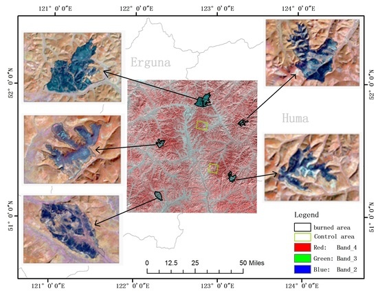
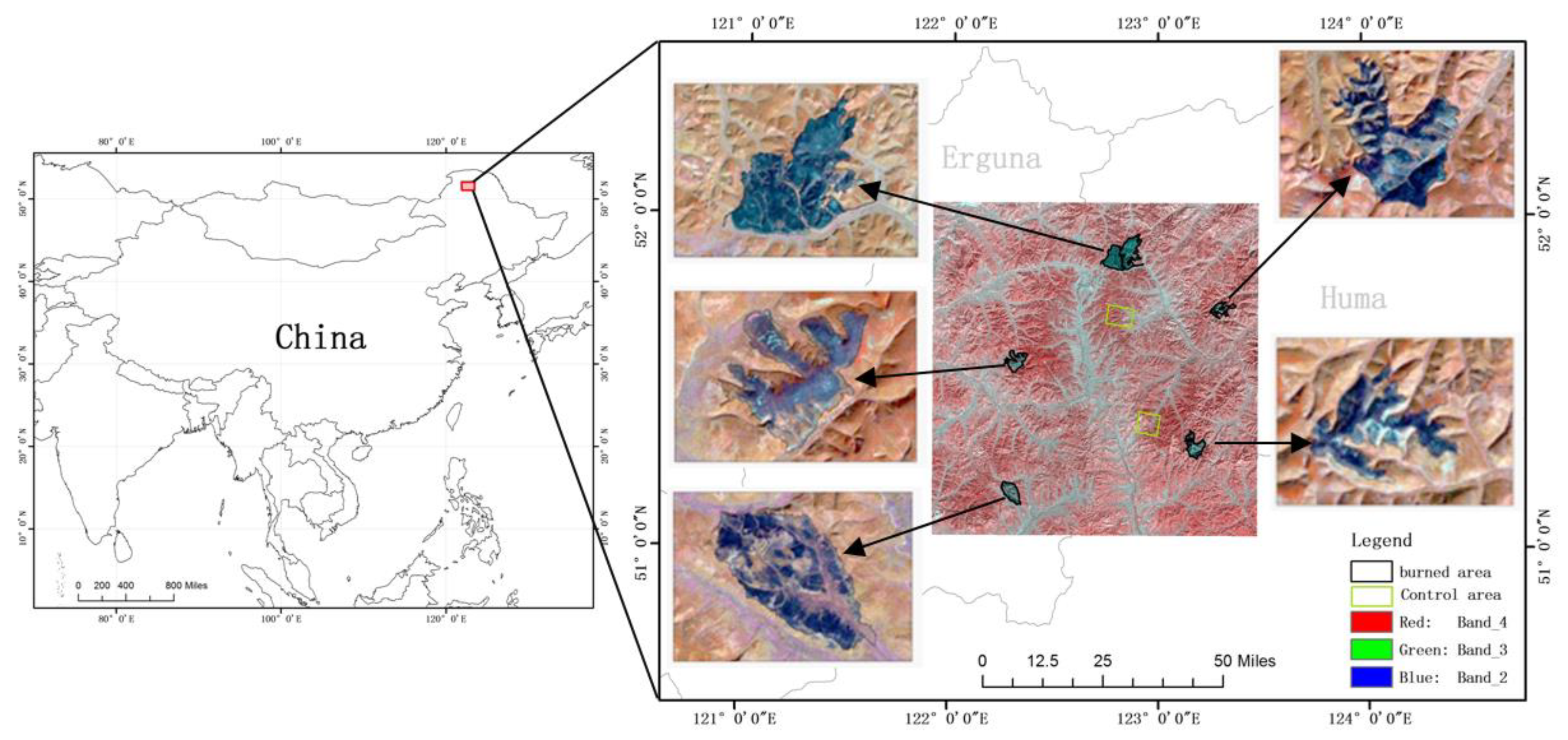
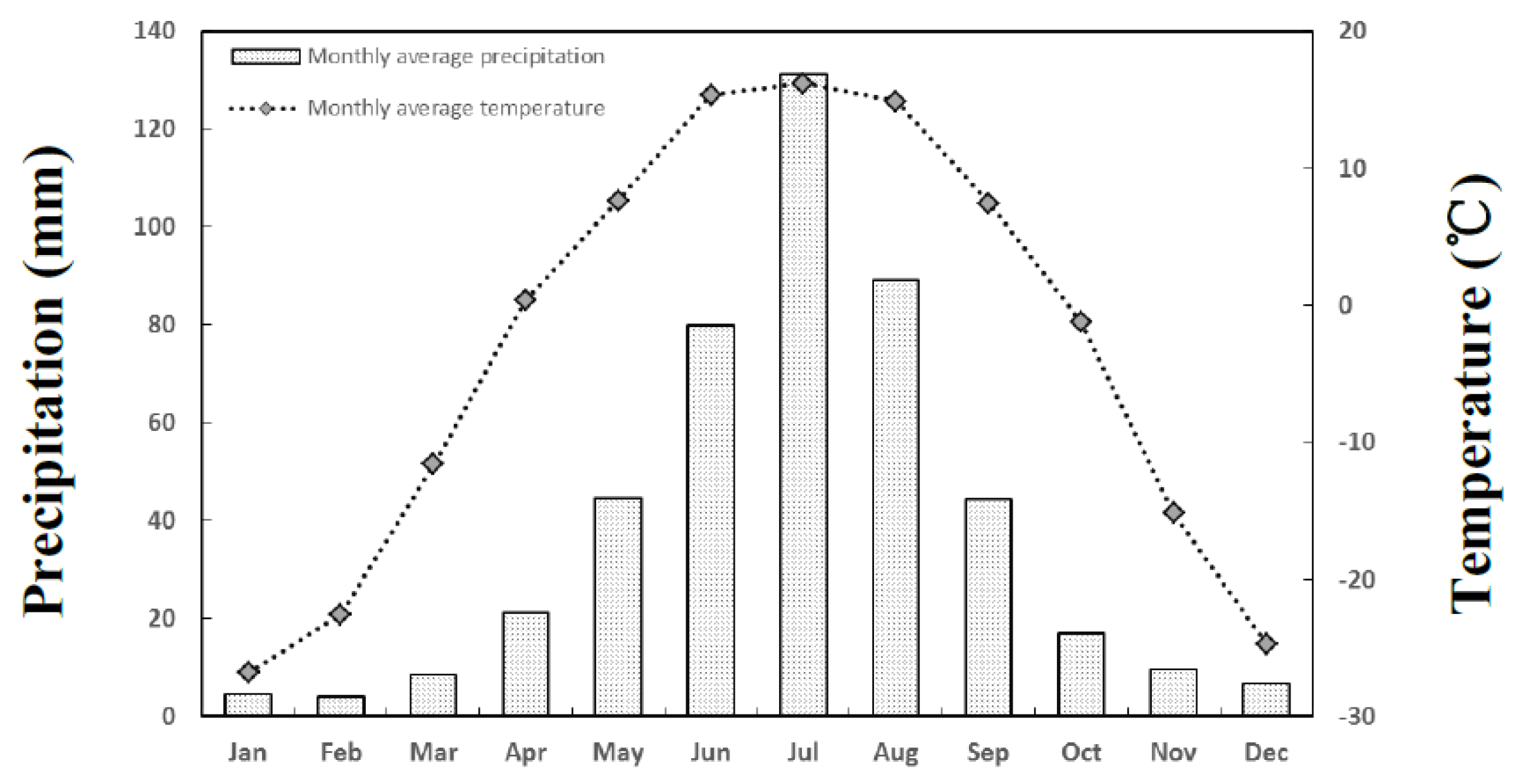
The five forest fires that were analyzed in this study occurred in the study area at almost the same time in June 2000. These fires were located in Northeast China (52°15′–53°33′N, 121°51′–125°05′E) along the border of Heilongjiang and Inner Mongolia (Figure 1) and burned more than eighteen thousand hectares of forest at different burn severities. The temporal and spatial extents and heterogeneity of the burn severities from this fire provide an ideal opportunity to study the effects of fire patterns on post-fire succession and their effect on the ecosystem’s energy flow. The terrestrial monsoon climate in this region produces short, mild summers (July’s average temperature is 16 °C) and long, severe winters (January’s average temperature is −26.8 °C). The annual precipitation amount is 461 mm, which is unevenly distributed throughout the year and peaks during summer (i.e., more than 60% occurs from June to August; see Figure 2). The species composition in this region is relatively simple but the forest cover is above 80%. The dominant tree species are larches, which are the southern extension of the eastern Siberian light-coniferous forest, and birches, which comprise approximately 10%. Other species include spruces, pines and two species of aspen [10,35].
2.2. Datasets
2.2.1. Landsat
Landsat time-series (1999–2016) images were downloaded from the US Geological Survey (USGS) website. We selected images with minimal cloud cover and acquisition dates within the growing season. The image ultimately met the criteria in Table 1. The Landsat TM and ETM+ data, which had higher spatial resolution (30 m), could more accurately express the spatial distribution characteristics of post-fire vegetation recovery. Therefore, we used these images to extract the fire areas and hierarchical burn severities and then compared the results with the MODIS data to verify the vegetation regeneration. The EVI enhances the vegetation signal by adding blue bands to correct for the effects of soil background and aerosol scattering, a procedure that was developed to resolve some of the limitations of the NDVI. The resulting coefficient was used to correct the variability in soil and canopy background reflectance, as shown in Equation (1):
where is the enhanced vegetation index and , are reflectance values of the blue, red and NIR bands, respectively.
2.2.2. MODIS
We obtained MODIS satellite-data-tile subsets from 2000 to 2016 from the Oak Ridge National Laboratory Distributed Active Archive Center (DACC; http://www.modis.ornl.gov/modis/index.cfm), alongside the EVI from the standard VI product (MOD13A1, 8-day, 500 m), the LSWI from the surface reflectance product (MOD09A1, 8-day, 500 m) and the LST from the land-surface temperature product (MOD11A2, 8-day, 1 km). The soil moisture and water-vapor pressure deficits are two main factors that directly determine the water contents of vegetation leaves, and the canopy ultimately affects vegetation photosynthesis. The LSWIs were derived from the NIR and SWIR bands, which are sensitive to vegetation’s water content and soil moisture [36,37,38], as shown in Equation (2):
where is the land-surface water index and are the reflectance values of the NIR and SWIR bands, respectively. The NIR and SWIR bands were derived from the MODIS 8-day surface reflectance product (MOD09A1), which included seven spectral bands. Band 2 (841–875 nm) and Band 6 (1628–1652 nm) are the NIR and SWIR bands, respectively. MOD17 is used to monitor global vegetation productivity and provides 8-day composites of the GPP, annual GPP and NPP at a 1-km resolution. Previous studies confirmed that no consistent overestimation or underestimation exists in MOD17 compared to the productivity from field-observed and flux-tower measurements. A direct validation comparison work on GPP (MOD17A3) that used 38 years of site-observation data showed a high correlation and low bias (r = 0.859 ± 0.173; relative error = 24%) [39]. However, MOD17 GPP and NPP still exhibit inaccuracies because of land cover, the FPAR, the LAI and daily meteorological values; these inputs contain substantial inaccuracies [39].
The preprocessing steps for the MODIS data in this study included constructing subset layers, transforming projections, creating subsets of the study area and creating continuous time series. The monthly data composite used the maximum value composite (MVC) criterion via the 8-day MODIS product. The annual dataset was synthesized by using the mean value during the growing season. A recent study highlighted the importance of the temporal dimension; even the spatial heterogeneity is sacrificed to some degree in low-resolution imagery [40]. This characteristic explains our choice of MODIS imagery, which satisfies the spatial resolution requirement with high temporal resolution.
2.2.3. Topography
The topographic information was mainly used to analyze the effect of the topography on vegetation restoration in this study. The topographic information was obtained from the Advanced Space-borne Thermal Emission and Reflection Radiometer (ASTER) global digital elevation model (GDEM) and downloaded from the National Aeronautics and Space Administration’s (NASA) Reverb Data Portal (http://reverb.echo.nasa.gov/). The estimated product accuracies for vertical and horizontal data were 20 m and 30 m, respectively, at a 95% confidence level [41]. During an aspect analysis in ArcGIS, orientations between NW (315) and NE (45) were classified as north-facing slopes and those between SE (135) and SW (225) were classified as south-facing slopes [42,43]. We mainly discuss the vegetation restoration effects on pixels within the burn scar areas on north- and south-facing slopes; pixels that did not fall within these ranges were excluded.
2.3. Methods
Mapping Fire Damage
The burn severity, which is defined as the degree of environmental change that is directly caused by fires, can be interpreted as the degree of degradation of the pre-fire vegetation community. The burn severity directly determines the rate of forest-regeneration [44]. Some studies show that the normalized burn ratio (NBR) is particularly useful for monitoring the burn severity. To ascertain the burn severity in conifer forests, the pre-NBR values are necessary as a control scenario. Here, the differenced normalized burn ratio (DNBR) was the spectral index that was applied to evaluate the burn severity [45,46]. The DNBR was calculated using Equation (4), and the NBR was calculated using Equation (3), where NIR and SWIR2 refer to the near infrared and shortwave infrared 2 bands 4 and 7, respectively, in the Landsat TM and ETM+ data:
where is the 1999 NBR value and NBRpost-fire is the NBR value in the fire year. The calculated DNBR was assigned to one of four levels based on the thresholds: high severity (DNBR ≥ 0.6), moderate severity (0.3 ≤ DNBR < 0.6), low severity (0.1 ≤ DNBR < 0.3) and unburned (DNBR < 0.1).
3. Results
3.1. Fire Damage Assessment
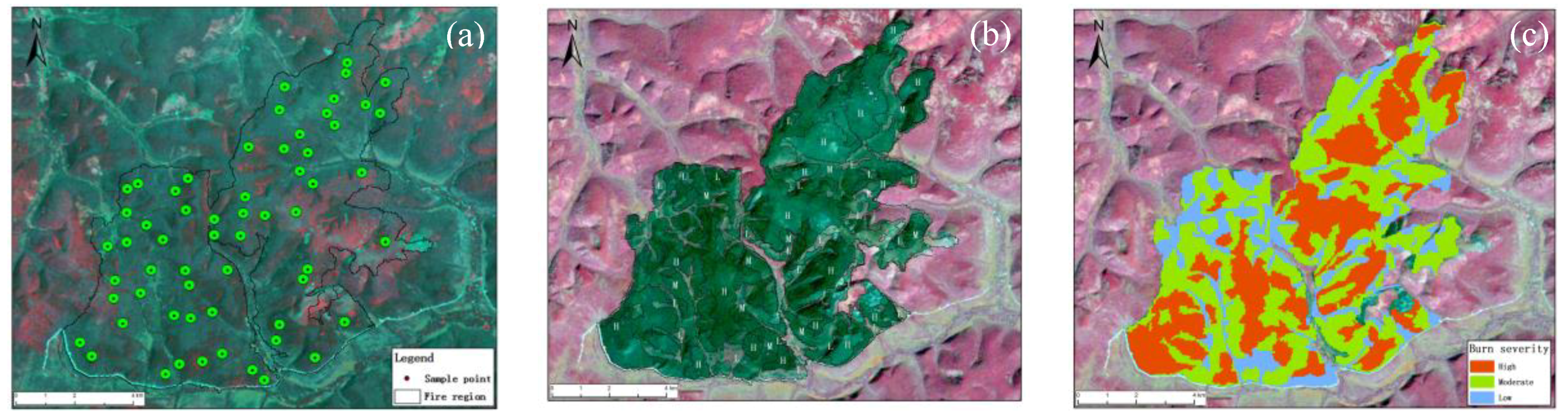
The spatial and temporal patterns of post-fire vegetation succession are determined by the climate conditions, the surrounding vegetation condition and topography. The burn severity influences the spatial configurations of forest patches, which, in turn, influence the ecological processes of post-fire recovery and succession. Hence, we must assess the burn severity to accurately track vegetation regeneration. The DNBR is the difference between the pre-fire NBR values and immediate post-fire values; this difference enabled us to identify the burn severity. We classified the burn severity in the study areas into four classes by using the DNBR method. Figure 3 shows one burn area’s DNBR spatial pattern as computed via Landsat images. The pre-fire spatial pattern of the land cover and the post-fire burn severity classification result in 2000 are illustrated in Figure 3a–c. The classification values, burned areas and percentages are illustrated in Table 2.
3.2. Temporal Analysis of the Post-Fire Vegetation Trajectory
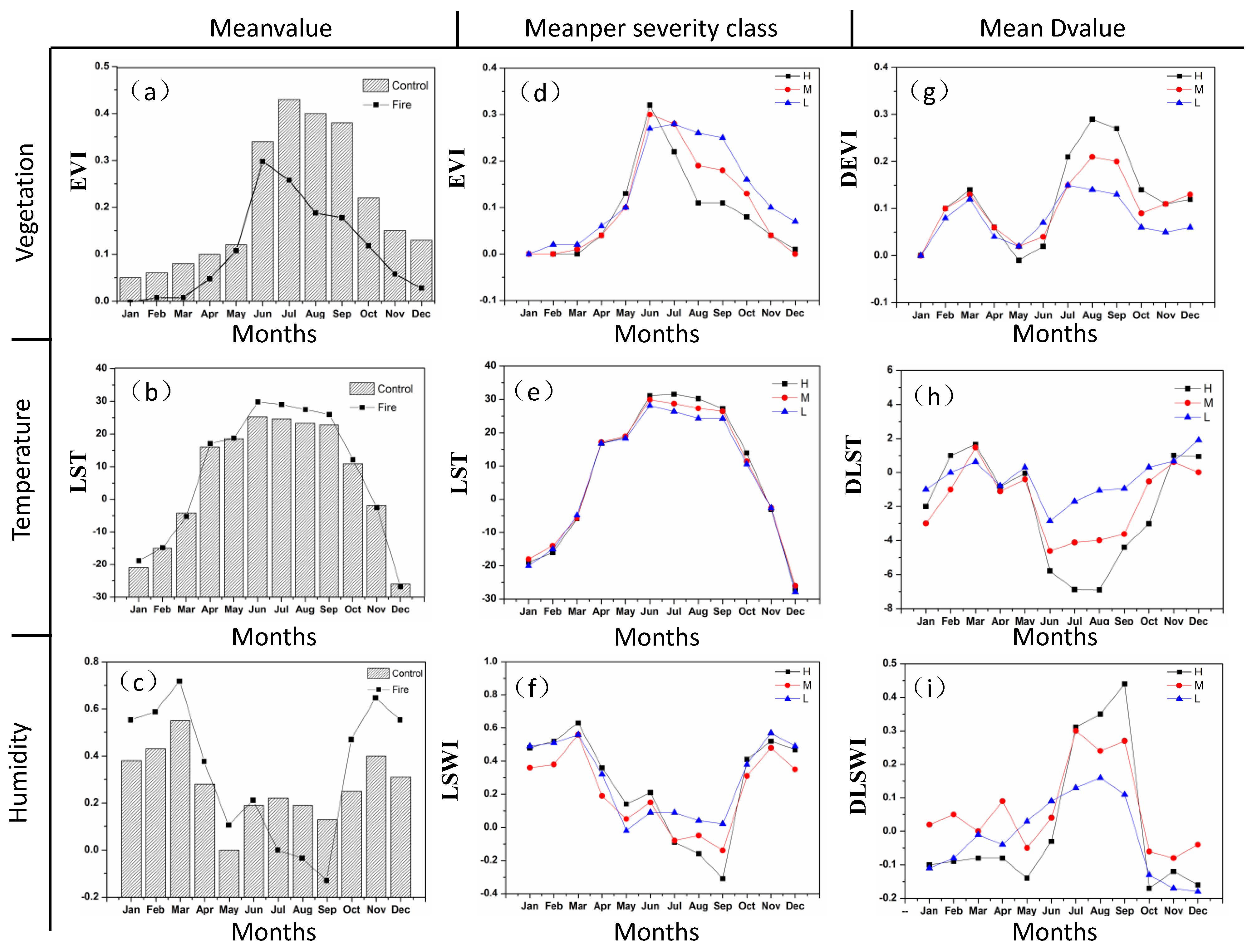
The following sections summarize the results of the intra-annual and inter-annual post-fire changes in the EVI, LST and LSWI (Figure 4 and Figure 5). The mean values of different burn severities in the five fire zones were used for analysis. In addition, we selected a non-fire area adjacent to the burned areas (Figure 1) as a control area to eliminate influences from climate change on the forest dynamics. Both the control area and burned areas had similar topographies and climate characteristics and had never experienced any other type of disturbance (e.g., artificial or natural disturbances). The variations in the EVI, LST and LSWI are illustrated in a series of statistical graphs (Figure 3). Figure 3a–c shows the annual changes via the burned- and control-pixel values. The mean values of the EVI and LST in the control pixels were unimodal (Figure 3a,b). The maximum LST was observed in June, and the EVI peaked in July. The LSWI value was the highest in winter, and the maximum value during the growing season occurred in July. Comparing the fire areas indicated immediate post-fire changes in the three indices: the EVI and LSWI decreased by 0.21 and 0.31, respectively, and the LST increased to 6.89 °C. The variations in the EVI and LSWI were more explicitly caused by the fire than those in the LST. Figure 3d–f displays the index variations under different fire intensities. The results clearly showed that the amplitude changes in the indices were controlled by the fire intensity, and the indices in the fire areas continued to reflect the original disturbance trends. The absolute values of the burned area and control area revealed that the greatest EVI difference occurred in August (a high difference of 0.29 in the severe-fire area). The largest LST and LSWI differences in the severe-fire area appeared in August and September, with differences of 6.9 and 0.44, respectively.
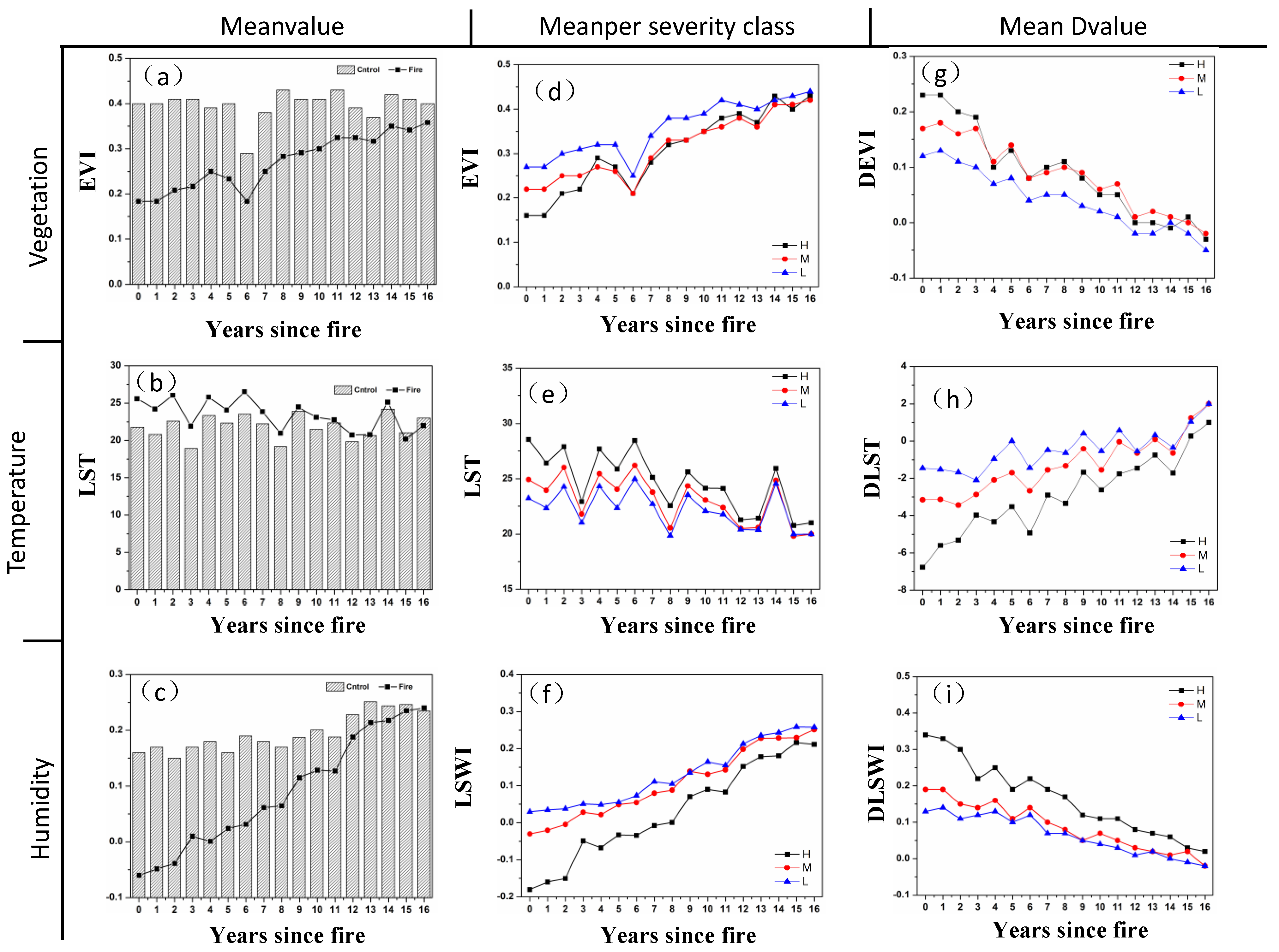
The temporal profiles of the EVI, LST and LSWI at different burn severity levels during the seventeen-year study period were extracted. An unburned region was selected as the control area for comparison to the burned sites (Figure 5). Changes in the EVI, LST and LSWI were not evident between the fire-occurrence year and the subsequent year, showing no obvious vegetation recovery. The index profiles dramatically increased in the second year following the fire, suggesting that the burned areas were not immediately covered by green vegetation after the fire. The EVI measures the proportion of pure green vegetation, but we could not confirm that the green vegetation was the same as the pre-fire vegetation; in other words, the EVI that was recovered after the fire could have consisted of grasses or shrubs, followed by broadleaf plants, which were the dominant species in the post-fire succession. Generally, grass quickly grew and reached high EVI values after several months. Dwarf shrubs reached biomass saturation within a relatively short period (5–7 years). Therefore, the rapid initial EVI increase was mainly caused by the regeneration of dwarf shrubs and understory grasses that survived the fire. The differences in the EVI were very large between the different fire damage intensities. We estimated the mean EVI recovery period for different fire intensities (approximately 10, 12 and 16 years). The recovery time of the LST was one year earlier than that of the EVI under different fire intensities. Figure 5 shows that the three fire intensity areas had temperature differences during the fire-occurrence years of 6.9, 3.2 and 1.5 °C, while the recovery period for different fire intensities was approximately 8, 11 and 15 years. The LSWI values in the fire-affected areas decreased by 0.13, 0.19 and 0.34. The effects of light and moderate fire intensities on the LSWI lasted 14 and 15 years, while the severe-fire area did not reach the reference area’s value at the end of the study period.
3.3. Time Series of the GPP and NPP
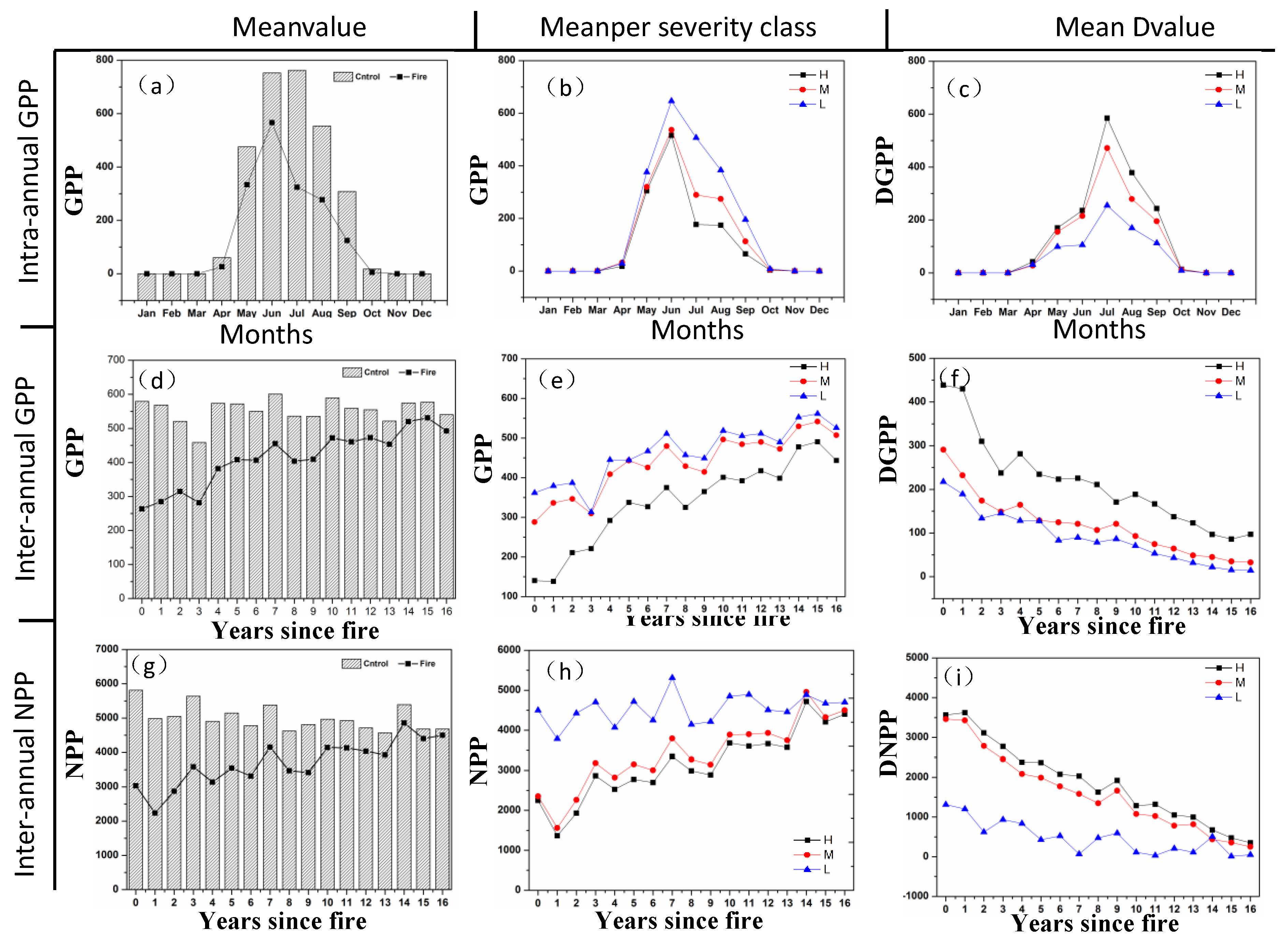
Similar annual distribution behaviors were apparent when comparing the GPP to the EVI and LST (Figure 6a). The GPP in the control area peaked in July and then dramatically decreased. The GPP was close to zero from October to March of the following year in the study area. In the burned areas, the GPP experienced a downward trend. A maximum difference of 50% occurred in the fire month or subsequent month (i.e., relative month 0 or 1). The GPP was also very low in the reference area during the winter because of seasonal effects; therefore, the GPP was mainly influenced by fires that occurred during the growing season.
The fire disturbances mainly influenced the GPP during the growing season (Figure 6a–c). Therefore, only the statistical GPP and NPP values from May to October were used in this study; the vegetation NPP and GPP decreased as the fire intensity increased. The GPP recovery rate was faster in earlier (1–3) years but became relatively slow in the fourth year of the recovery, and the GPP and NPP did not recover to their original levels during the 17-year study period. However, the GPP and NPP recovery times in the moderately and lightly burned areas were similar. The temporal profiles of the NPP linearly increased with a gradually decreasing slope but did not reach a steady state during the study period. Previous research showed that a steady state is not reached until at least 20 years after a fire, with a longer full-recovery period for the Alberta Boreal Plains eco-zone.
3.4. Relationships among MODIS Products with GPP and NPP Fluxes
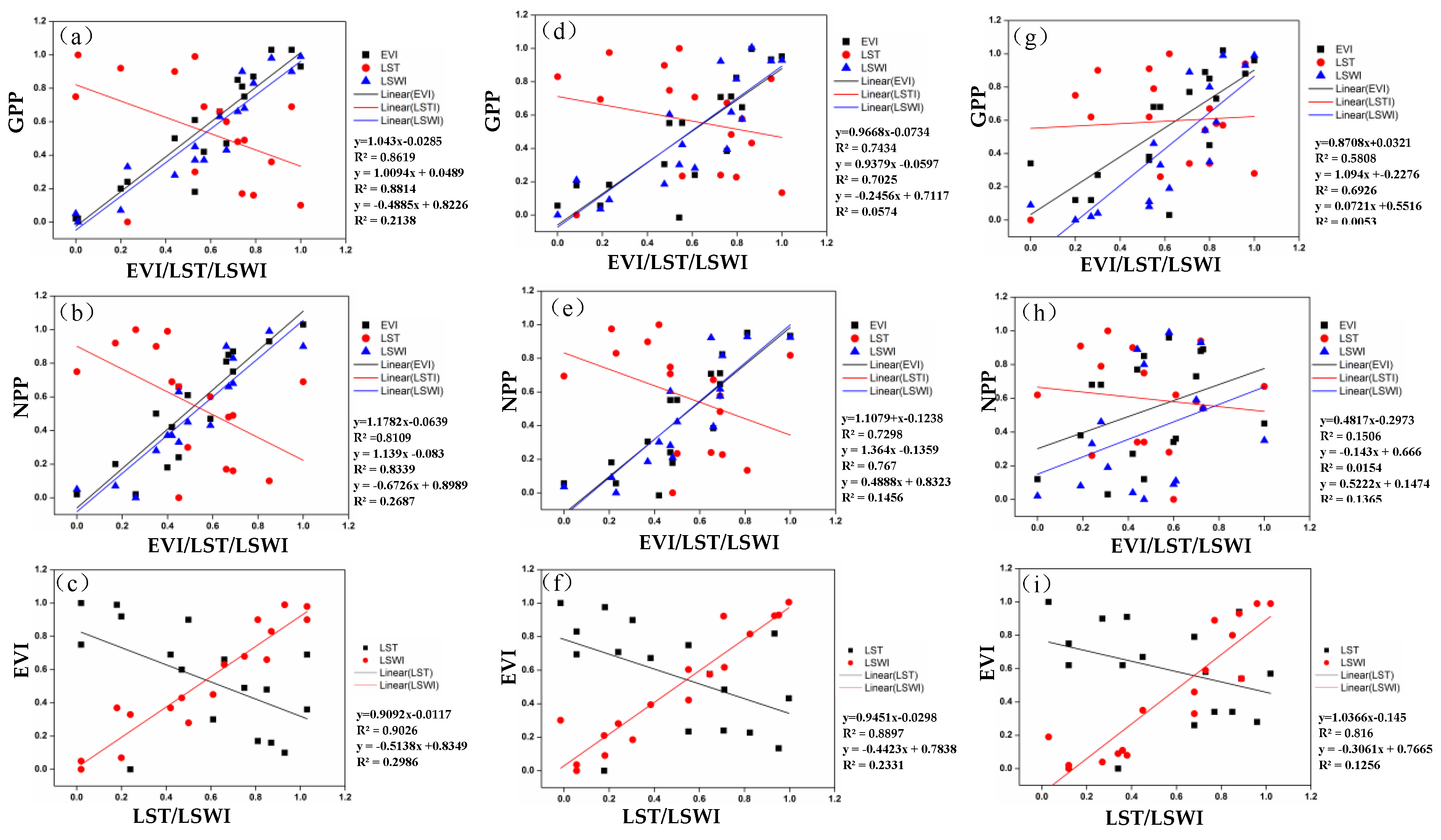
Figure 7a–f shows a series of scatter plots, which illustrate the relationship between the MODIS products (EVI, LSWI and LST) and GPP/NPP flux data values from linear-regression analysis. In most of the models, the effects of water and temperature on plant photosynthesis were estimated as a relationship function. Thus, we explored the relationships between the LSWI-EVI and LST-EVI to determine an inter-relationship that could yield more information on vegetation succession (Figure 7g–i). We calculated the average annual values based on the different burn severities to obtain the correlations for the multiyear data. The results in Figure 7 show that the correlations of the EVI and LSWI with the GPP/NPP were greater than those of the LST. The correlations were strongest in the high-severity fire areas; the correlation coefficients with the EVI were 0.86 and 0.81, respectively, and those with the LSWI were 0.88 and 0.83, respectively. As the burn severity weakened, the correlation coefficient also gradually fell. The LST and GPP had a negative correlation, but this correlation was not strong. At all burn severities, the EVI-LSWI correlations of the sites were positive and the EVI-LST correlations were negative, but the EVI-LSWI relationships appeared to be stronger than the EVI-LST relationships; as the fire intensity weakened, the correlation coefficient decreased from 0.9 to 0.81.
4. Discussion
4.1. Temporal Analysis of the Post-Fire Vegetation Trajectory
In this study, the EVI was used to measure the vegetation growth and the LST and LSWI were used to monitor the post-fire hydrothermal conditions. Therefore, analysis of post-fire forest-regeneration trajectories with the EVI, LST and LSWI was expected to reveal different characteristics of post-fire forest-successional processes and patterns. Figure 4 confirms the utility of the MODIS (EVI, LST and LSWI) data for monitoring fire-induced vegetation changes because the data yielded different results at different burn severities (see Figure 6, Figure 7 and Figure 8). The magnitude of the changes in the LSWI and LST was significant and closely related to the burn severity, as reflected in the EVI changes (see Figure 6, Figure 7 and Figure 8). The annual time-series values of the indices, however, were also subject to seasonal variations. The changes in the MODIS index were minor in winter because of weak vegetation activity, which produced imperceptible changes from fire disturbances. The average EVI value in the focal pixels with high burn severity was 0.21 less than that in the control pixels. The results were very similar, changing from 0.15 to 0.35 [9]. The mean of the focal pixels exceeded the mean of the control pixels by 1.1–6.9 °C, similar to the 2–8 °C immediate post-fire temperature increase during the daytime that has been reported by other studies [29,47,48,49,50]. In this study, the EVI continued to decrease and the LST continued to increase during the second month after the fire (Figure 4); however, no clear recovery trend was evident during the next two years (Figure 5). This result differed from previous research results, where the EVI and LST immediately fell after recovery. This difference might have been related to the location of the fire region, specifically, a boreal forest in a northern region, whose cold climate, strong seasonality and short growing season result in slower recovery times. The greatest differences in the EVI, LST and LSWI were observed in August and September, which were not the fire month or the next month. The results showed that the seasonality aggravated the effects of fire interference. Additionally, the changes in the LST depend on the burn severity and meteorological conditions, which limits the ability of the LST to characterize vegetation changes after fire disturbances [23,24,25].
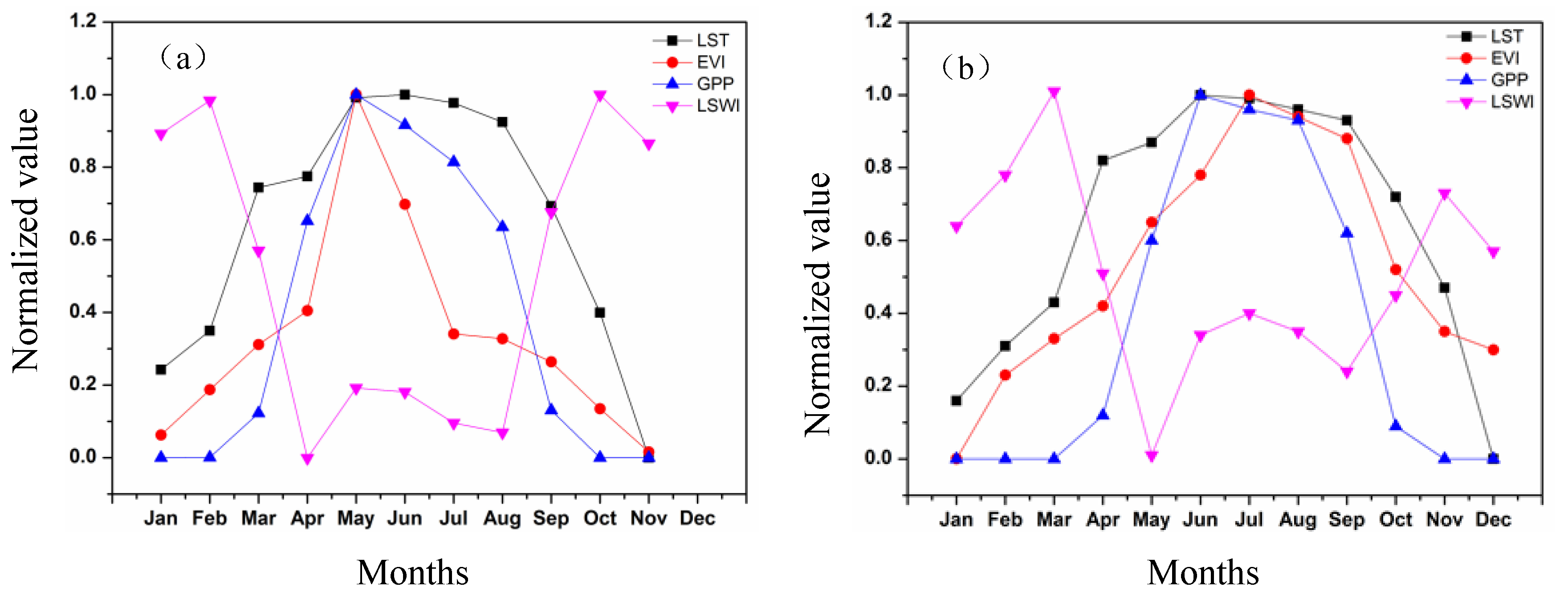
4.2. Comparisons of the Seasonal Dynamics of Biophysical Profiles on Post-Fire Areas
Although the post-fire EVI, LST and LSWI changes were consistent with the results from previous studies [29,47,50,51], few prior studies incorporated seasonal changes and fewer still compared and analyzed index differentials and relationships. In this study, four remote sensing indices (after normalization) were used to perform a comparative analysis of the annual changes from fire disturbance and seasonality. The regional climate is known to determine seasonal cycles. An extended period of snow cover and a short growing season are obvious features of boreal forests; in particular, this study measured significant unique seasonal changes in the EVI, LST and LSWI. The maximum intra-annual temperature was the highest in July because of insolation effects (Figure 2). However, the maximum LST was observed in June, and the EVI peaked in July, which decreased July’s LST. The effects of fires on vegetation activities and energy flow were difficult to observe during winter because the EVI and GPP values reached a minimum (close to zero) for the entire seasonal cycle, even in the control area. The LST and LSWI’s yearly maximum and minimum values are mainly affected by winter-snow conditions, which do not meet the requirements for photosynthesis. The LST began to increase in March, but the GPP, EVI and LSWI did not increase until April. Temperature is the limiting factor for vegetation growth. Figure 8 shows the immediate post-fire changes in the EVI, LST and LSWI, but the EVI changes were clearly more persistent than those of the LSWI and LST. The integrated analysis of the LST and LSWI suggested that fire created a more arid environment, which reduced the effect of climate, as demonstrated with the higher LST and lower LSWI. In addition, the effect of fires in winter is small, but fires can still have an effect. We found that the post-fire EVI values were lower than those of the control area in winter, indicating that fires affected the evergreen forest. The GPP value was 0, suggesting that the MODIS could only roughly record the energy flow.
4.3. Post-Fire Energy Fluxes
As shown in Figure 6, the temporal profiles of the NPP and GPP values in the control area illustrated that the NPP and GPP in mature boreal forest communities are 0.58 kg C·m−2·year−1 and 58 g C·m−2·month−1, which are similar to the flux-tower determination results of 0.6 kg C·m−2·year−1 [52]. Post-fire succession significantly affected the canopy structure and LAI, reflecting an alteration of the energy balance and evapotranspiration and modifying the latent heat flux (LE). In this study, the GPP and NPP decreased by approximately 26–58 g C·m−2·month−1 and 0.23–0.45 kg C·m−2·year−1, respectively, following a fire (Figure 6). Based on fire-regeneration studies, most tree seedlings are established during the 3–10 year period following a fire, while shrub regeneration occurs in 6–7 years [53]. However, the EVI was the result of shrub and ground vegetation growth in the early post-fire years (Figure 10). The GPP and NPP recovered faster during the first three years, with a second turning point during Years 6–7, which matches the vegetation succession process. The conceptual model showed that the NPP and GPP remained low during the early post-fire succession stage; the recovery peaked in the early and mid-succession stages and then decreased or remained steady at the end of the succession, when the vegetation reached maturity or an older stage. The NPP and GPP reached a steady state in the control area, but the NPP and GPP values in the focal areas continued to rise, even at the end of the entire 17-year study period. These results confirmed prior reports that post-fire GPP and NPP reach relatively steady states only after 20 years or longer. In reality, achieving a steady state could require 20–60 years, and the required time increases with increasing latitude and correspondingly colder temperatures [53], such as in the taiga boreal forest eco-zone. Without a longer dataset for these areas, we could not reliably predict when a steady state might be reached for the study area, but the NPP and GPP values were close to zero in the sixteenth year, suggesting that a steady state should be attained within a few more years. In addition, the NPP and GPP post-fire recovery trajectories were well illustrated by this method, which showed that the steady state period and degradation process could be inverted and were feasible beyond the limited local information from ground measurements.
4.4. Relationship of MODIS Products to the GPP and NPP
GPP can be directly estimated on a per-pixel basis from MODIS EVI data at a broad scale [31]. Nevertheless, the strong correlations between EVI and GPP/NPP in Figure 3 confirmed that the C-flux of post-fire vegetation succession could be estimated with fairly high accuracy by using the overall relationship. Pearson’s correlation coefficient (r) under different burn severities suggested that the relationships were not static and were affected by the burn severity. Our data results suggest that the EVI provides a simple but robust approach for estimating post-fire GPP and NPP and thus has similar potential for light-use-efficiency and data-driven models. The relationships between the LSWI-GPP and LSWI-NPP were stronger because the strong correlation between the EVI and LSWI supported this relationship. In addition, previous studies confirmed that the potential of this method for estimating terrestrial GPP is similar to that when using the MOD17 GPP and NPP datasets [54,55]. No measured data were available in the fire study area, so this study could not easily conclude that the EVI had the potential to estimate terrestrial GPP during vegetation recovery.
4.5. Other Factors that Affected Post-Fire Recovery
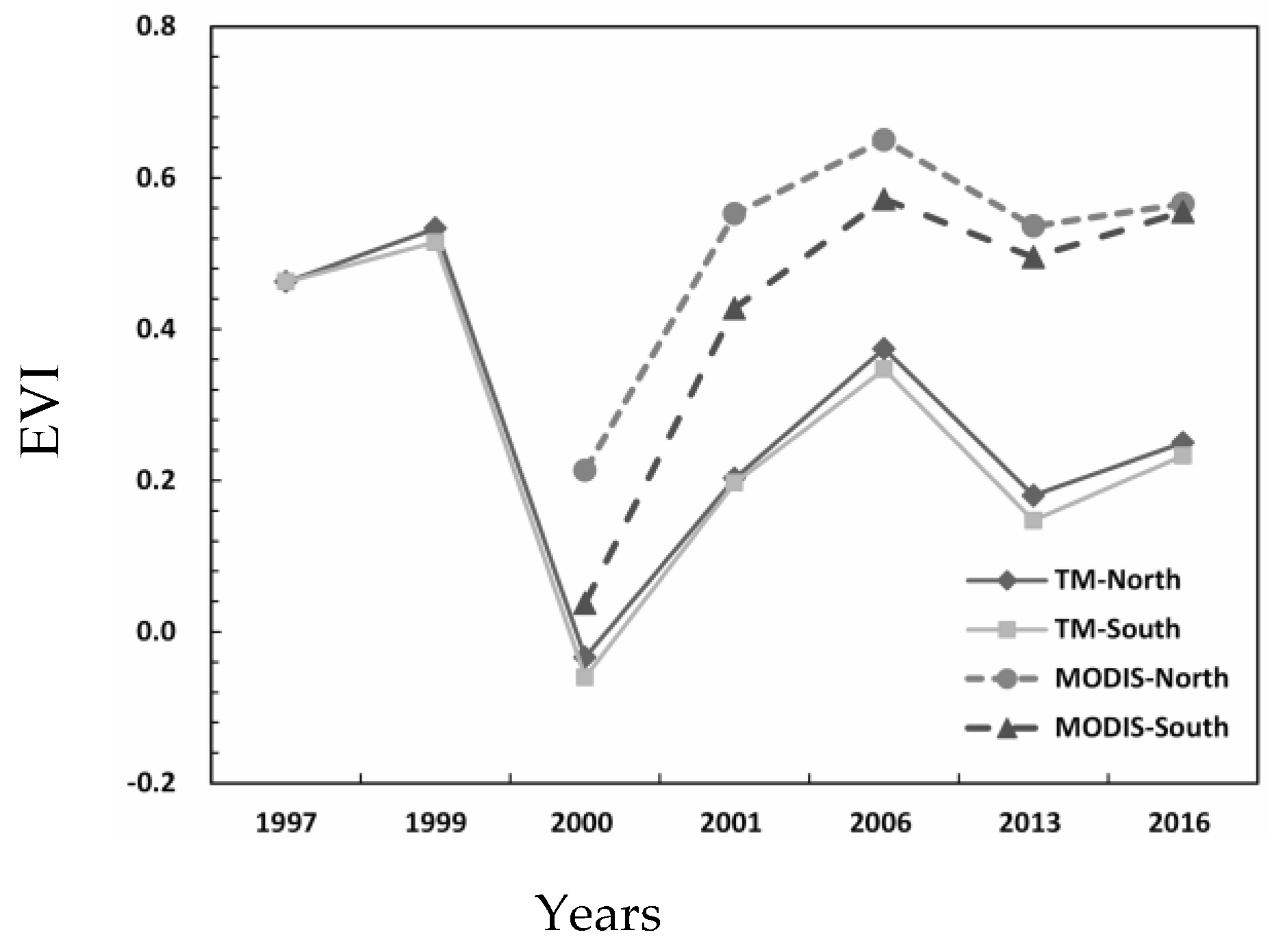
The higher spatial resolution of Landsat TM/ETM+ sensors enables the temporal and spatial characteristics of fire recovery processes to be more precisely delineated, and these factors can be used simultaneously to assess the accuracy of the MODIS data. The selected Landsat images were acquired during the growing season, when the vegetation restoration characteristics were most obvious. The MODIS 8-day images that were closest to the Landsat samples’ acquisition dates were selected to ensure that the data had comparable temporal resolution. Figure 9 shows similar EVI trends in the post-fire vegetation regeneration via MODIS and Landsat. Positive bias appeared in the MODIS dataset compared to the Landsat EVI values. This result confirms that the MODIS dataset overestimated the EVI for post-fire vegetation regeneration in this region. This result likely occurred because the MODIS EVI primarily consisted of maximum acquisitions.
The EVI is a universal indicator of vegetation’s fractional coverage and growth conditions [38]. The Landsat TM data responded to spatial-recovery characteristics in detail (Figure 9), and the results showed the topographic effect on the vegetation recovery dynamics, particularly the investigated aspects. Table 3 and Figure 10 present the results from the examination of the response of vegetation regrowth to topography after the fire. The EVI appeared to decrease immediately after the fire in both the northern and southern regions, and subsequent regeneration also appeared in both areas but exhibited a faster rate along the northern region compared to the southern region. This same conclusion has been reported by other studies within the Northern Hemisphere [43,56,57]. The dates of the results indicate that the topography plays a key role in post-fire vegetation succession. The differences reflect the importance of local hydrological variability and soil hydrophobicity to post-fire vegetation regeneration.
4.6. Uncertainty Analysis
Boreal forests are subject to fire disturbances, and climate change will increase the frequency of fires. The EVI, LST and LSWI dramatically changed after the fire, and the seasonality aggravated changes in the magnitude. The short growing seasons at high latitudes limit annual tree growth and severe winters control the time of forest succession, so the seasonality primarily controls the land-surface energy fluxes during vegetation regeneration. In this paper, the results confirmed the correlation between the EVI and GPP/NPP from MODIS. The rough data resolution and simple estimation method added considerable uncertainty to the estimation results. Surface energy flow is a more complex process, especially during vegetation regeneration. Therefore, we must improve the data resolution and the accuracy of the model algorithm to estimate the influence of vegetation succession on the carbon flux.
5. Conclusions
This study conducted a pixel-based analysis of post-fire vegetation trajectories and changes in surface energy fluxes after a 2000 boreal forest wildfire over a 17-year post-fire period based on MODIS satellite imagery. The burned area underwent natural succession. The EVI, LST and LSWI dramatically changed after the fire, with the changes in the EVI being clearly more persistent. Therefore, the EVI was the most effective at detecting burns and distinguishing severity levels. Longer-term changes in the EVI, LST and LSWI greatly depended on the seasonality, confirming that the seasonality is another important factor that affects vegetation restoration and land-surface energy fluxes in boreal forests. The strong EVI-GPP and EVI-NPP correlations in this paper demonstrated these factors’ potential for use as an alternative method to estimate the GPP (even in a post-fire recovery area), monitor land-surface energy fluxes during vegetation restoration and reduce uncertainties in the estimation of forests’ carbon reserves. This study utilized Landsat images to provide detailed spatially continuous and quantitative estimations of the vegetation recovery and demonstrate the influence of topography, which is a key parameter that controls the physical processes in fire-altered areas. The topography affected vegetation restoration by changing the hydrothermal conditions, which further affected the carbon-distribution pattern of the recovering vegetation.
Research on post-fire vegetation restoration and carbon flow should involve large areas and a long time span. Therefore, performing real field validations is usually not feasible for such a study. Future research will approach the relationships between vegetation regeneration and the C-flux in boreal forest ecosystems by using multi-temporal remote sensing techniques. In addition, rough data resolution and simple estimation methods add considerable uncertainty to the estimation results, and the degree of fire interference on boreal forests in different seasons exhibits significant differences. Therefore, more detailed satellite analyses and field data are required in the future to improve the validation of results.
Author Contributions
All authors contributed to the conception and design of this research and the discussion of results. X.L., the principal author of the manuscript, was responsible for the collection, analysis and interpretation of the data. H.Z., the corresponding author, was responsible for the experimental concepts. G.Y. and Y.D. contributed the analysis tools and reviewed the manuscript. J.Z. was responsible for manuscript revision.
Funding
This research was funded by the National Natural Science Foundation of China (Grant Nos. 41771450, 41501449, 41501408, 41361091 and 41571489), the National Science and Technology Major Project of China (Grant No. 2015ZX07201-008-10), the Fundamental Research Funds for the Central Universities (Grant No. 2412017FZ021) and the Guizhou Provincial Science and Technology Program Project (Grant No. 2015[4007]).
Conflicts of Interest
The authors declare no conflicts of interest.
References
- Janhäll, S.; Andreae, M.O.; Pöschl, U. Biomass burning aerosol emissions from vegetation fires: Particle number and mass emission factors and size distributions. Atmos. Chem. Phys. Discuss. 2009, 9, 808–813. [Google Scholar] [CrossRef]
- Mike, F.; Brian, S.; Merritt, T.; Mike, W. Impacts of climate change on fire activity and fire management in the circumboreal forest. Glob. Chang. Biol. 2009, 15, 549–560. [Google Scholar]
- Balshi, M.S.; Mcguire, A.D.; Duffy, P.; Flannigan, M.; Kicklighter, D.W.; Melillo, J. Vulnerability of carbon storage in North American boreal forests to wildfires during the 21st century. Glob. Chang. Biol. 2009, 15, 1491–1510. [Google Scholar] [CrossRef] [Green Version]
- Zhan, S.; Di, X.; Hui, H. Effects to Forest Fire Occurrence of Climate Change in Ta He Forestry Bureau in Great Xing’an Mountain. In Proceedings of the 2011 International Conference on Environmental Biotechnology and Materials Engineering, Harbin, China, 26–28 March 2011; pp. 135–139. [Google Scholar]
- Liu, Z.; Yang, J.; Chang, Y.; Weisberg, P.J.; He, H.S. Spatial patterns and drivers of fire occurrence and its future trend under climate change in a boreal forest of Northeast China. Glob. Chang. Biol. 2012, 18, 2041–2056. [Google Scholar] [CrossRef]
- Cai, W.; Yang, J.; Liu, Z.; Hu, Y.; Weisberg, P.J. Post-fire tree recruitment of a boreal larch forest in Northeast China. For. Ecol. Manag. 2013, 307, 20–29. [Google Scholar] [CrossRef]
- Hagemann, U.; Moroni, M.T.; Shaw, C.H.; Kurz, W.A.; Makeschin, F. Comparing measured and modelled forest carbon stocks in high-boreal forests of harvest and natural-disturbance origin in Labrador, Canada. Ecol. Model. 2010, 221, 825–839. [Google Scholar] [CrossRef]
- Meng, R.; Wu, J.; Zhao, F.; Cook, B.D.; Hanavan, R.P.; Serbin, S.P. Measuring short-term post-fire forest recovery across a burn severity gradient in a mixed pine-oak forest using multi-sensor remote sensing techniques. Remote Sens. Environ. 2018, 210, 282–296. [Google Scholar] [CrossRef]
- Veraverbeke, S.; Verstraeten, W.W.; Lhermitte, S.; Kerchove, R.V.D.; Goossens, R. Assessment of post-fire changes in land surface temperature and surface albedo, and their relation with fire–burn severity using multitemporal MODIS imagery. Int. J. Wildland Fire 2012, 21, 243–256. [Google Scholar] [CrossRef]
- Yi, K.; Tani, H.; Zhang, J.; Guo, M.; Wang, X.; Zhong, G. Long-term satellite detection of post-fire vegetation trends in boreal forests of China. Remote Sens. 2013, 5, 6938–6957. [Google Scholar] [CrossRef]
- Johnstone, J.F.; Iii, F.S.C.; Foote, J.; Kemmett, S.; Price, K.; Viereck, L. Decadal observations of tree regeneration following fire in boreal forests. Rev. Can. Rech. For. 2004, 34, 267–273. [Google Scholar] [CrossRef]
- Johnstone, J.F.; Rupp, T.S.; Olson, M.; Verbyla, D. Modeling impacts of fire severity on successional trajectories and future fire behavior in Alaskan boreal forests. Landsc. Ecol. 2011, 26, 487–500. [Google Scholar] [CrossRef]
- Aakala, T.; Pasanen, L.; Helama, S.; Vakkari, V.; Drobyshev, I.; Seppä, H.; Kuuluvainen, T.; Stivrins, N.; Wallenius, T.; Vasander, H. Multiscale variation in drought controlled historical forest fire activity in the boreal forests of eastern Fennoscandia. Ecol. Monogr. 2018, 88, 74–91. [Google Scholar] [CrossRef]
- Cuevas-gonzález, M.; Gerard, F.; Balzter, H.; Riaño, D. Analysing forest recovery after wildfire disturbance in boreal Siberia using remotely sensed vegetation indices. Glob. Chang. Biol. 2009, 15, 561–577. [Google Scholar] [CrossRef]
- Man, C.D.; Nguyen, T.T.; Bui, H.Q.; Lasko, K.; Nguyen, T.N.T. Improvement of land-cover classification over frequently cloud-covered areas using Landsat 8 time-series composites and an ensemble of supervised classifiers. Int. J. Remote Sens. 2018, 39, 1243–1255. [Google Scholar] [CrossRef]
- Epting, J.; Verbyla, D. Landscape-level interactions of prefire vegetation, burn severity, and postfire vegetation over a 16-year period in interior Alaska. Can. J. For. Res. 2005, 35, 1367–1377. [Google Scholar] [CrossRef]
- Jones, M.O.; Kimball, J.S.; Jones, L.A. Satellite microwave detection of boreal forest recovery from the extreme 2004 wildfires in Alaska and Canada. Glob. Chang. Biol. 2013, 19, 3111–3122. [Google Scholar] [CrossRef] [PubMed]
- Jin, Y.; Randerson, J.T.; Goetz, S.J.; Beck, P.S.A.; Loranty, M.M.; Goulden, M.L. The influence of burn severity on postfire vegetation recovery and albedo change during early succession in North American boreal forests. J. Geophys. Res. Biogeosci. 2015, 117, 1–8. [Google Scholar] [CrossRef]
- Hicke, J.A.; Asner, G.P.; Kasischke, E.S.; French, N.H.F.; Randerson, J.T.; Collatz, G.J.; Stocks, B.J.; Tucker, C.J.; Los, S.O.; Field, C.B. Postfire response of North American boreal forest net primary productivity analyzed with satellite observations. Glob. Chang. Biol. 2003, 9, 1145–1157. [Google Scholar] [CrossRef] [Green Version]
- Chu, T.; Guo, X.; Takeda, K. Remote sensing approach to detect post-fire vegetation regrowth in Siberian boreal larch forest. Ecol. Indic. 2016, 62, 32–46. [Google Scholar] [CrossRef]
- Cuevas-González, M.; Gerard, F.; Balzter, H.; Riaño, D. Studying the change in fAPAR after forest fires in Siberia using MODIS. Int. J. Remote Sens. 2008, 29, 6873–6892. [Google Scholar] [CrossRef] [Green Version]
- Kasischke, E.S.; Nhf, F.; Harrell, P.; Nljr, C.; Ustin, S.L.; Barry, D. Monitoring of wildfires in boreal forests using large area AVHRR NDVI composite image data. Remote Sens. Environ. 1993, 45, 61–71. [Google Scholar] [CrossRef]
- Goetz, S.J.; Sun, M.; Baccini, A.; Beck, P.S.A. Synergistic use of spaceborne lidar and optical imagery for assessing forest disturbance: An Alaska case study. J. Geophys. Res. Biogeosci. 2015, 115, 471–478. [Google Scholar] [CrossRef]
- Chu, T.; Guo, X. Remote Sensing Techniques in monitoring post-fire effects and patterns of forest recovery in boreal forest regions: A Review. Remote Sens. 2013, 6, 470–520. [Google Scholar] [CrossRef]
- Wang, S.; Ibrom, A.; Bauer-Gottwein, P.; Garcia, M. Incorporating diffuse radiation into a light use efficiency and evapotranspiration model: An 11-year study in a high latitude deciduous forest. Agric. For. Meteorol. 2018, 248, 479–493. [Google Scholar] [CrossRef]
- Monteith, J.L. Solar Radiation and Productivity in Tropical Ecosystems. J. Appl. Ecol. 1972, 9, 747–766. [Google Scholar] [CrossRef]
- Tepley, A.J.; Thompson, J.R.; Epstein, H.E.; Anderson-Teixeira, K.J. Vulnerability to forest loss through altered postfire recovery dynamics in a warming climate in the Klamath Mountains. Glob. Chang. Biol. 2017, 23, 4117–4132. [Google Scholar] [CrossRef] [PubMed]
- Amiro, B.D.; Orchansky, A.L.; Barr, A.G.; Black, T.A.; Chambers, S.D.; Fsiii, C.; Goulden, M.L.; Litvak, M.; Liu, H.P.; Mccaughey, J.H. The effect of post-fire stand age on the boreal forest energy balance. Agric. For. Meteorol. 2006, 140, 41–50. [Google Scholar] [CrossRef] [Green Version]
- Montes-Helu, M.C.; Kolb, T.; Dore, S.; Sullivan, B.; Hart, S.C.; Koch, G.; Hungate, B.A. Persistent effects of fire-induced vegetation change on energy partitioning and evapotranspiration in ponderosa pine forests. Agric. For. Meteorol. 2009, 149, 491–500. [Google Scholar] [CrossRef]
- Sánchez, J.; Bisquert, M.; Rubio, E.; Caselles, V. Impact of land cover change induced by a fire event on the surface energy fluxes derived from remote sensing. Remote Sens. 2015, 7, 14899–14915. [Google Scholar] [CrossRef]
- Shi, H.; Li, L.; Eamus, D.; Huete, A.; Cleverly, J.; Tian, X.; Yu, Q.; Wang, S.; Montagnani, L.; Magliulo, V. Assessing the ability of MODIS EVI to estimate terrestrial ecosystem gross primary production of multiple land cover types. Ecol. Indic. 2017, 72, 153–164. [Google Scholar] [CrossRef]
- Sims, D.A.; Rahman, A.F.; Cordova, V.D.; El-Masri, B.Z.; Baldocchi, D.D.; Flanagan, L.B.; Goldstein, A.H.; Hollinger, D.Y.; Misson, L.; Monson, R.K. On the use of MODIS EVI to assess gross primary productivity of North American ecosystems. J. Geophys. Res. Biogeosci. 2015, 111, 695–702. [Google Scholar] [CrossRef]
- Wu, Z.W.; He, H.S.; Chang, Y.; Liu, Z.H.; Chen, H.W. Development of customized fire behavior fuel models for boreal forests of northeastern China. Environ. Manag. 2011, 48, 1148. [Google Scholar] [CrossRef] [PubMed]
- Turner, M.G.; Romme, W.H.; Gardner, R.H.; Hargrove, W.W. Effects of fire size and pattern on early succession in Yellowstone National Park. Ecol. Monogr. 1997, 67, 411–433. [Google Scholar] [CrossRef]
- Li, X.; He, H.S.; Wu, Z.; Liang, Y.; Schneiderman, J.E. Comparing effects of climate warming, fire, and timber harvesting on a boreal forest landscape in Northeastern China. PLoS ONE 2013, 8, e59747. [Google Scholar] [CrossRef] [PubMed]
- Huete, A.R. Soil-dependent spectral response in a developing plant canopy. Agron. J. 1987, 79, 61. [Google Scholar] [CrossRef]
- Xiao, X.; Hollinger, D.; Aber, J.; Goltz, M.; Davidson, E.A.; Zhang, Q.; Iii, B.M. Satellite-based modeling of gross primary production in an evergreen needleleaf forest. Remote Sens. Environ. 2004, 89, 519–534. [Google Scholar] [CrossRef]
- Xiao, X.; Hollinger, D.; Aber, J.; Moore, B. Modeling gross primary production of an evergreen needleleaf forest using modis and climate data. Ecol. Appl. 2005, 15, 954–969. [Google Scholar] [CrossRef]
- Martel, M.C.; Margolis, H.A.; Coursolle, C.; Bigras, F.J.; Heinsch, F.A.; Running, S.W. Decreasing photosynthesis at different spatial scales during the late growing season on a boreal cutover. Tree Physiol. 2005, 25, 689–699. [Google Scholar] [CrossRef] [PubMed] [Green Version]
- Veraverbeke, S.; Harris, S.; Hook, S. Evaluating spectral indices for burned area discrimination using MODIS/ASTER (MASTER) airborne simulator data. Remote Sens. Environ. 2011, 115, 2702–2709. [Google Scholar] [CrossRef]
- Tachikawa, T.; Hato, M.; Kaku, M.; Iwasaki, A. Characteristics of ASTER GDEM version 2. In Proceedings of the Geoscience and Remote Sensing Symposium, Vancouver, BC, Canada, 24–29 July 2011; pp. 3657–3660. [Google Scholar]
- Petropoulos, G.P.; Griffiths, H.M.; Kalivas, D.P. Quantifying spatial and temporal vegetation recovery dynamics following a wildfire event in a Mediterranean landscape using EO data and GIS. Appl. Geogr. 2014, 50, 120–131. [Google Scholar] [CrossRef]
- Wittenberg, L.; Dan, M.; Beeri, O.; Halutzy, A.; Tesler, N. Spatial and temporal patterns of vegetation recovery following sequences of forest fires in a Mediterranean landscape, Mt. Carmel Israel. Catena 2007, 71, 76–83. [Google Scholar] [CrossRef]
- Lentile, L.B.; Holden, Z.A.; Smith, A.M.S.; Falkowski, M.J.; Hudak, A.T.; Morgan, P.; Lewis, S.A.; Gessler, P.E.; Benson, N.C. Remote sensing techniques to assess active fire characteristics and post-fire effects. Int. J. Wildland Fire 2006, 15, 319–345. [Google Scholar] [CrossRef]
- Wimberly, M.C.; Reilly, M.J. Assessment of fire severity and species diversity in the southern Appalachians using Landsat TM and ETM+ imagery. Remote Sens. Environ. 2007, 108, 189–197. [Google Scholar] [CrossRef] [Green Version]
- Wagtendonk, J.W.V.; Root, R.R.; Key, C.H. Comparison of AVIRIS and Landsat ETM+ detection capabilities for burn severity. Remote Sens. Environ. 2004, 92, 397–408. [Google Scholar] [CrossRef]
- Wendt, C.K.; Beringer, J.; Tapper, N.J.; Hutley, L.B. Local boundary-layer development over burnt and unburnt tropical savanna: An observational study. Bound.-Layer Meteorol. 2007, 124, 291–304. [Google Scholar] [CrossRef]
- García, M.J.L.; Caselles, V. Mapping burns and natural reforestation using thematic Mapper data. Geocarto Int. 2008, 6, 31–37. [Google Scholar] [CrossRef]
- Cahoon, D.R.; Stocks, B.J.; Levine, J.S.; Cofer, W.R.; Pierson, J.M. Satellite analysis of the severe 1987 forest fires in northern China and southeastern Siberia. J. Geophys. Res. Atmos. 1994, 99, 18627–18638. [Google Scholar] [CrossRef]
- Lambin, E.F.; Goyvaerts, K.; Petit, C. Remotely-sensed indicators of burning efficiency of savannah and forest fires. Int. J. Remote Sens. 2003, 24, 3105–3118. [Google Scholar] [CrossRef]
- Lyons, E.A.; Jin, Y.; Randerson, J.T. Changes in surface albedo after fire in boreal forest ecosystems of interior Alaska assessed using MODIS satellite observations. J. Geophys. Res. Biogeosci. 2015, 113, 912. [Google Scholar] [CrossRef]
- Goulden, M.L.; Mcmillan, A.M.S.; Winston, G.C.; Rocha, A.V.; Manies, K.L.; Harden, J.W.; Bond-Lamberty, B.P. Patterns of NPP, GPP, respiration, and NEP during boreal forest succession. Glob. Chang. Biol. 2011, 17, 855–871. [Google Scholar] [CrossRef] [Green Version]
- Amiro, B.D.; Chen, J.M.; Liu, J. Net primary productivity following forest fire for Canadian ecoregions. Rev. Can. Rech. For. 2000, 30, 939–947. [Google Scholar] [CrossRef]
- Wang, L.; Zhu, H.; Lin, A.; Zou, L.; Qin, W.; Du, Q. Evaluation of the latest MODIS GPP products across multiple biomes using Global Eddy Covariance Flux Data. Remote Sens. 2017, 5. [Google Scholar] [CrossRef]
- Gebremichael, M.; Barros, A.P. Evaluation of MODIS Gross Primary Productivity (GPP) in tropical monsoon regions. Remote Sens. Environ. 2006, 100, 150–166. [Google Scholar] [CrossRef]
- Cerdà, A.; Doerr, S.H. The influence of vegetation recovery on soil hydrology and erodibility following fire: An eleven-year investigation. Int. J. Wildland Fire 2005, 14, 423–437. [Google Scholar] [CrossRef]
- Fox, D.M.; Maselli, F.; Carrega, P. Using SPOT images and field sampling to map burn severity and vegetation factors affecting post forest fire erosion risk. Catena 2008, 75, 326–335. [Google Scholar] [CrossRef]
Figure 1.
Location of the study area (the background image is a thematic mapper (TM) image from 2000).
Figure 1.
Location of the study area (the background image is a thematic mapper (TM) image from 2000).

Figure 2.
Average temperature and precipitation diagram between the Tulihe (Yakeshi and Hulunbuir) and Xinlin (DaXingAnLing and Heilongjiang) meteorological stations from 2000 to 2016 via the national meteorological science data-sharing service platform (http://data.cma.cn/).
Figure 2.
Average temperature and precipitation diagram between the Tulihe (Yakeshi and Hulunbuir) and Xinlin (DaXingAnLing and Heilongjiang) meteorological stations from 2000 to 2016 via the national meteorological science data-sharing service platform (http://data.cma.cn/).

Figure 3.
Fire damage map of the study area, with fire damage values obtained using Equation (4). Sample points were used to identify fire pixels for subsequent analysis. These sample points were selected to be as distant as possible within the fire intensity area to avoid interference from different burn severities. One study site before (a) and after a fire (b) and a severity map of the 2000 burned area were derived from the bi-temporal image-differencing approach via the normalized burn ratio (DNBR), with the 1999 Landsat TM as the pre-fire image and the 2000 severity map as the post-fire image (c).

Figure 4.
Temporal trajectories of the post-fire vegetation recovery and seasonal dynamics as defined by the EVI, LST and LSWI between the control area and fire area at different burn severity levels. EVI’s annual dynamics in the control and focal pixels (a); EVI’s dynamics under different fire intensities (d); EVI’s differences between the control and focal pixels under different fire intensities (g); LST’s annual dynamics in the control and fire pixels (b); LST under different fire intensities (e); LST’s difference between the control and focal pixels (h); LSWI’s annual dynamics in the control and focal pixels (c); LSWI under different fire intensities annually (f); and LSWI’s differences between the control and focal pixels (i).

Figure 5.
Temporal trajectories of the post-fire forest recovery as defined by the growing season average (May to October) of the EVI, LST and LSWI between the control area and focal area at different burn severity levels. EVI’s annual dynamics in the control and focal pixels (a); EVI’s dynamics under different fire intensities (d); EVI’s difference between the control and focal pixels (g); LST’s annual dynamics in the control and focal pixels (b); LST under different fire intensities (e); LST’s differences between the control and focal pixels (h); LSWI’s annual dynamics in the control and focal pixels (c); LSWI under different fire intensities annually (f); and LSWI’s differences between the control and focal pixels (i).

Figure 6.
Variation trajectories of GPP and NPP in post-fire forests. (a–c) represent the annual changes in the GPP. Theinter-annual trajectories of: GPP (d–f); and NPP (g–i). GPP and NPP’s differences between the control and focal pixels (a,d,g); inter-annual trajectories under different fire intensities (b,e,h); and differences under different fire intensities between the control and focal pixels (c,f,i).

Figure 7.
Comparison of the correlation between the MODIS index products (EVI, LSWI and LST) and C-flux data (GPP and NPP) under difference burn severities: (a–c) high burn severity; (d–f) moderate burn severity; and (g–i) light burn severity. The correlation between EVI and GPP was slightly higher than those of the other parameters.

Figure 8.
Annual seasonal profiles of the EVI, LST, LSWI and GPP for the control and focal pixels after normalization processing: (a) focal pixels; and (b) control pixels. Remote sensing indices (after normalization) were used to perform a comparative analysis of the annual changes from fire disturbances and seasonality.

Figure 9.
Comparison between the MODIS EVI and Landsat EVI. The curves represent the EVI profiles along the north-facing and south-facing slopes for MODIS and Landsat, respectively.
Figure 9.
Comparison between the MODIS EVI and Landsat EVI. The curves represent the EVI profiles along the north-facing and south-facing slopes for MODIS and Landsat, respectively.

Figure 10.
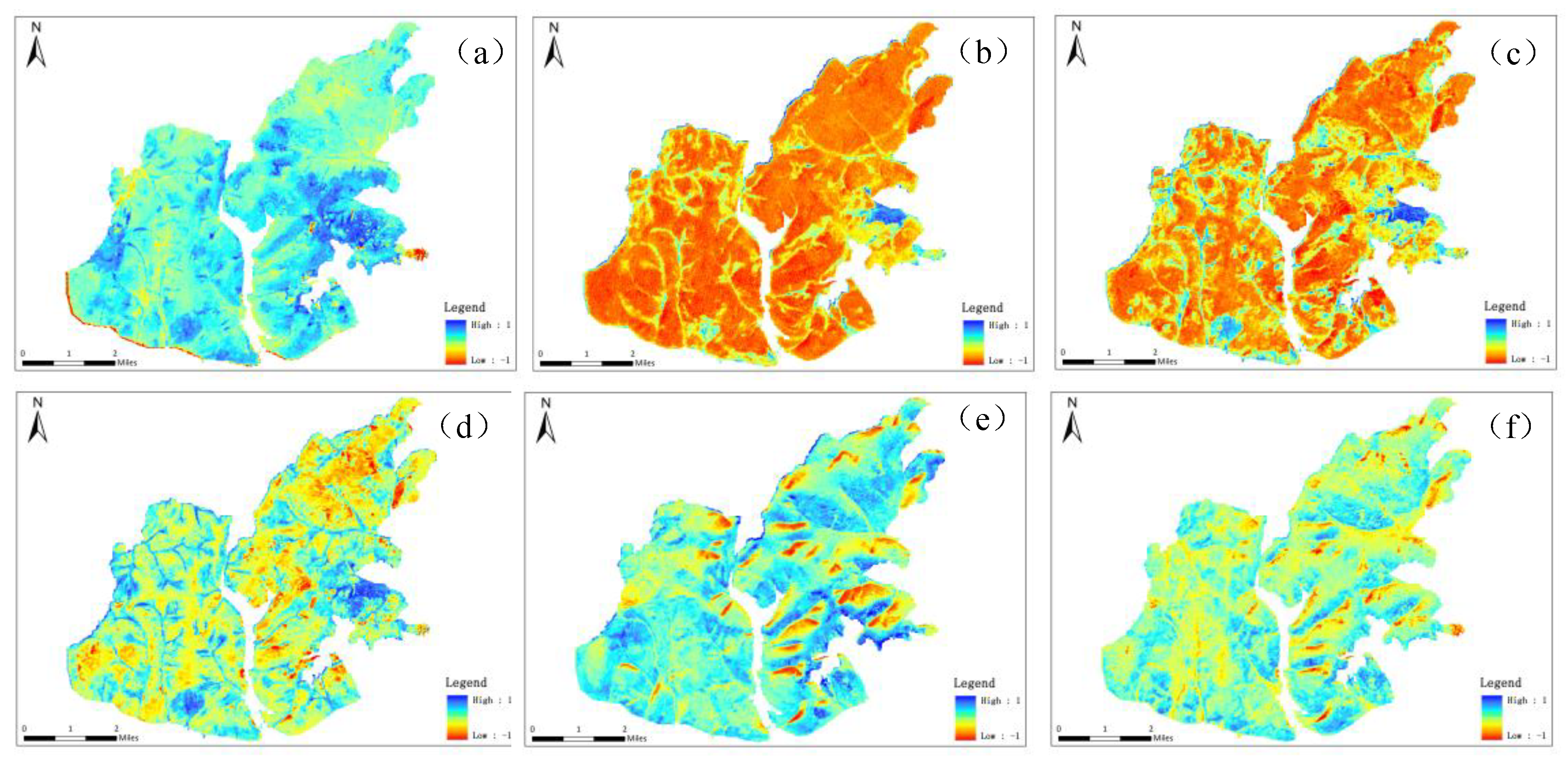
Examples of the EVI estimation based on Landsat data via a pre-fire image (1999 (a)) and post-fire images ((b–f) represent 2000, 2001, 2006, 2014 and 2016; the spatial pattern in 2004 was similar to that in 2006 and thus was not included). The temporal and spatial characteristics of the EVI illustrate fire-related changes in ground vegetation. The locations of these five tracked samples are shown in Figure 4. The minus and plus signs represent the pre-fire and post-fire periods, respectively. Fire damage classes: High (H), Moderate (M) and Slight (S).
Figure 10.
Examples of the EVI estimation based on Landsat data via a pre-fire image (1999 (a)) and post-fire images ((b–f) represent 2000, 2001, 2006, 2014 and 2016; the spatial pattern in 2004 was similar to that in 2006 and thus was not included). The temporal and spatial characteristics of the EVI illustrate fire-related changes in ground vegetation. The locations of these five tracked samples are shown in Figure 4. The minus and plus signs represent the pre-fire and post-fire periods, respectively. Fire damage classes: High (H), Moderate (M) and Slight (S).


Table 1.
Landsat TM and ETM+ scenes that were used in this analysis. Time-series Landsat images were used to assess the post-fire recovery forests in Northeast China. All images were acquired from the same path (column 122 and row 23).
Table 1.
Landsat TM and ETM+ scenes that were used in this analysis. Time-series Landsat images were used to assess the post-fire recovery forests in Northeast China. All images were acquired from the same path (column 122 and row 23).
| ID | Acquisition Date | Years Since the Fire |
|---|---|---|
| 1 | 3 August 1999 | Pre-fire |
| 2 | 14 September 2000 | Fire year |
| 3 | 23 July 2001 | 1 |
| 4 | 15 July 2004 | 4 |
| 5 | 6 August 2006 | 6 |
| 6 | 2 August 2014 | 14 |
| 7 | 22 August 2016 | 16 |
Table 2.
Fire damage classification when using the DNBR method.
| Fire Damage Class | DNBR | Area (km2) | SD | Percentage (%) | |
|---|---|---|---|---|---|
| Unburned | <0.1 | 101.33 | 0.07 | 0.02 | / |
| Low | 0.1–0.3 | 68.42 | 0.25 | 0.04 | 37.70% |
| Moderate | 0.3–0.6 | 59.59 | 0.42 | 0.03 | 32.83% |
| High | >0.6 | 53.48 | 0.68 | 0.04 | 29.47% |
Table 3.
Descriptive statistics for the EVI throughout the study area in the burn scar along the north- and south-facing slopes.
Table 3.
Descriptive statistics for the EVI throughout the study area in the burn scar along the north- and south-facing slopes.
| Landsat TM Image Data | Minimum EVI | Maximum EVI | Mean EVI | Standard Deviation |
|---|---|---|---|---|
| (a) North-facing slopes only | ||||
| August 1999 (Pre-fire) | −0.066 | 0.887 | 0.675 | 0.120 |
| September 2000 | −0.080 | 0.885 | 0.182 | 0.150 |
| July 2001 | −0.133 | 0.88 | 0.256 | 0.138 |
| July 2004 | −0.095 | 0.877 | 0.422 | 0.095 |
| August 2006 | −0.109 | 0.872 | 0.44 | 0.126 |
| August 2014 | −0.114 | 0.886 | 0.692 | 0.122 |
| August 2016 | −0.05 | 0.882 | 0.673 | 0.127 |
| (b) South-facing slopes only | ||||
| August 1999 (Pre-fire) | −0.032 | 0.887 | 0.614 | 0.146 |
| September 2000 | −0.012 | 0.865 | 0.165 | 0.140 |
| July 2001 | −0.126 | 0.881 | 0.272 | 0.125 |
| July 2004 | −0.013 | 0.845 | 0.377 | 0.097 |
| August 2006 | −0.09 | 0.865 | 0.412 | 0.128 |
| August 2014 | −0.117 | 0.876 | 0.622 | 0.122 |
| August 2016 | −0.103 | 0.885 | 0.627 | 0.132 |
© 2018 by the authors. Licensee MDPI, Basel, Switzerland. This article is an open access article distributed under the terms and conditions of the Creative Commons Attribution (CC BY) license (http://creativecommons.org/licenses/by/4.0/).
Share and Cite
MDPI and ACS Style
Li, X.; Zhang, H.; Yang, G.; Ding, Y.; Zhao, J. Post-Fire Vegetation Succession and Surface Energy Fluxes Derived from Remote Sensing. Remote Sens. 2018, 10, 1000. https://0-doi-org.brum.beds.ac.uk/10.3390/rs10071000
AMA Style
Li X, Zhang H, Yang G, Ding Y, Zhao J. Post-Fire Vegetation Succession and Surface Energy Fluxes Derived from Remote Sensing. Remote Sensing. 2018; 10(7):1000. https://0-doi-org.brum.beds.ac.uk/10.3390/rs10071000
Chicago/Turabian StyleLi, Xuedong, Hongyan Zhang, Guangbin Yang, Yanling Ding, and Jianjun Zhao. 2018. "Post-Fire Vegetation Succession and Surface Energy Fluxes Derived from Remote Sensing" Remote Sensing 10, no. 7: 1000. https://0-doi-org.brum.beds.ac.uk/10.3390/rs10071000
Note that from the first issue of 2016, this journal uses article numbers instead of page numbers. See further details here.