Article

Multispectral Pansharpening with Radiative Transfer-Based Detail-Injection Modeling for Preserving Changes in Vegetation Cover

1
Department of Information Engineering and Mathematics, University of Siena, 53100 Siena, Italy
2
Institute of Applied Physics “Nello Carrara”, IFAC-CNR, Research Area of Florence, 50019 Sesto Fiorentino (FI), Italy
3
Department of Information Engineering, University of Florence, 50139 Florence, Italy
4
Institute of Methodologies for Environmental Analysis, CNR–IMAA, 85050 Tito Scalo (PZ), Italy AND NASA-JCET, Greenbelt, MD 20771, USA
5
Department of Information Engineering, Electrical Engineering and Applied Mathematics, University of Salerno, 84084 Fisciano (SA), Italy
*
Author to whom correspondence should be addressed.
Submission received: 27 July 2018 / Revised: 9 August 2018 / Accepted: 9 August 2018 / Published: 19 August 2018
(This article belongs to the Section Forest Remote Sensing)

Abstract

:
Whenever vegetated areas are monitored over time, phenological changes in land cover should be decoupled from changes in acquisition conditions, like atmospheric components, Sun and satellite heights and imaging instrument. This especially holds when the multispectral (MS) bands are sharpened for spatial resolution enhancement by means of a panchromatic (Pan) image of higher resolution, a process referred to as pansharpening. In this paper, we provide evidence that pansharpening of visible/near-infrared (VNIR) bands takes advantage of a correction of the path radiance term introduced by the atmosphere, during the fusion process. This holds whenever the fusion mechanism emulates the radiative transfer model ruling the acquisition of the Earth’s surface from space, that is for methods exploiting a multiplicative, or contrast-based, injection model of spatial details extracted from the panchromatic (Pan) image into the interpolated multispectral (MS) bands. The path radiance should be estimated and subtracted from each band before the product by Pan is accomplished. Both empirical and model-based estimation techniques of MS path radiances are compared within the framework of optimized algorithms. Simulations carried out on two GeoEye-1 observations of the same agricultural landscape on different dates highlight that the de-hazing of MS before fusion is beneficial to an accurate detection of seasonal changes in the scene, as measured by the normalized differential vegetation index (NDVI).

Graphical Abstract

1. Introduction

The term panchromatic sharpening or pansharpening denotes the process by which the geometric resolution of a multi-band image is increased by means of a single-band panchromatic observation of the same scene having greater spatial resolution. Pansharpening techniques take advantage of the complementary spatial and spectral resolutions of multi-/hyper-spectral (MS/HS) and panchromatic (Pan) images to synthesize a unique fusion product that exhibits as many spectral bands as the MS/HS image, each with the same spatial resolution as the Pan image [1,2]. It is important, however, to highlight that pansharpening cannot increase the spatial resolution of the spectral information of the original data, but is simply a means to represent such information at a finer spatial scale, more suitable for visual or automated analysis tasks [3].
Recent achievements in MS pansharpening mostly exploit the concept of superresolution [4]. Despite the formal mathematical elegance of some approaches, all such methods exhibit very subtle increments in performance (decrements, in some cases [5]) over the state-of-the-art, obtained at an exorbitant computational cost of massive constrained numerical minimizations, with plenty of adjustable parameters. Superresolution-based, or more generally optimization-based, variational methods, either model-based [6] or not [7], are unconceivable for practical applications requiring routine fusion of tens of megapixels of data, for which traditional approaches are pursued [3]. Especially, their performance is crucial, being subordinated to a proper optimization of its running parameters on a local basis, e.g., on small blocks partially overlapped to avoid discontinuities in fusion effects. What was believed would become the third generation of pansharpening methods is still far to come.
Conversely, the current second generation of pansharpening methods, which approximately started twenty years ago and was established ten years later [8], features methods all following the same flowchart. After the MS bands have been superimposed, that is interpolated and co-registered, to the Pan image, the spatial details of each pixel are extracted from the latter and added to the MS bands according to a certain injection model. The detailed extraction step can follow the spectral approach, originally known as component substitution (CS), or the spatial approach, which may rely on multiresolution analysis (MRA) [9], but not necessarily on a linear shift-invariant filtering, e.g., on morphological filtering [10]. The Pan image is preliminarily histogram matched, that is radiometrically transformed by constant gain and offset in such a way that its low-pass version, having the same spatial frequency content as the MS bands, exhibits mean and variance equal to those of the spectral component that shall be replaced, e.g., the intensity component, for CS methods, or the MS band that shall be sharpened for MRA methods [11,12,13].
The injection model rules the combination of the low-pass MS image with the spatial detail extracted from Pan. Such a model is stated between each of the co-registered MS bands and the low-pass version of the Pan image. A wide variety of injection models has been proposed in the literature [14,15]. However, the most popular ones are:
(i)
the projection model, which may be derived from the Gram–Schmidt (GS) orthogonalization procedure, representing the basis of the GS spectral sharpening [16] and of the context-based decision (CBD) [17];
(ii)
the multiplicative or contrast-based model, which is the basis of such techniques as high-pass modulation (HPM) [18], Brovey transform (BT) [19], the synthetic variable ratio (SVR) [20], UNBpansharp [21], smoothing filter-based intensity modulation (SFIM) [22] and the spectral distortion minimizing (SDM) injection model [23].
Unlike the projection model, which may be either global, as for GS, or local [24], as for CBD, the contrast-based model is inherently local, or context-adaptive [25,26], because the injection gain changes at each pixel [27]. The multiplicative injection model of details is the key to the fusion of MS images with synthetic aperture radar (SAR) images [28].
Although considerations of atmospheric effects were already present in SVR [20] and unspecified empirical adjustments in the baseline of UNB pansharp [21], the paper that introduced SFIM [22] firstly gave an interpretation of the multiplicative injection model in terms of the radiative transfer model ruling the acquisition of an MS image from a real-world scene [29]: a low spatial-resolution spectral reflectance, previously estimated from the MS bands and the low-pass filtered Pan image, is sharpened through multiplication by a high spatial-resolution solar irradiance, represented by the high-resolution Pan image.
Currently, very few authors [30,31,32,33] have explicitly considered the path radiance of the MS band, which is an undesired energy scattered by different atmospheric constituents that reaches the aperture of the instrument without being reflected by the Earth’s surface. Such an atmospheric path-radiance, which appears as haze in an RGB true color visualization, should be estimated and subtracted from each band before modulation and possibly re-inserted later, to get an unbiased sharpened image. The pansharpened bands are left de-hazed in all cases, in which spectral reflectance or analogous products are calculated.
Calculation of path-radiances may follow image-based approaches or rely on models of the atmosphere and its constituents, as well as on knowledge of acquisition parameters, such as actual Sun-Earth distance, Sun height angle and observation angle of the satellite platform. Image-based atmospheric corrections [34,35] are a series of statistical methods based on some general assumptions and empirical criteria (see Section 6.4). The goal is that of estimating the atmospheric effects on acquisition without requiring acquisition parameters or making assumptions on atmospheric constituents.
In this paper, after deriving the haze-corrected versions of contrast-based spectral (CS) and spatial (MRA) pansharpening methods, starting from physical considerations of radiative transfer, several methods for estimating the path radiances of individual bands are reviewed. Image-based and model-based estimates of path-radiances are correlated. For this purpose, the Fu–Liou–Gu (FLG) radiative transfer model [36] has been considered. Model-enforced empirical image-based haze estimation criteria attain the fusion performance of the theoretical model and of an exhaustive search for the unknown path-radiance values, performed at a degraded spatial scale [37]. Experiments carried out on a couple of GeoEye-1 images of the same agricultural landscape on different dates highlight that the de-hazing of MS is beneficial for an accurate detection of seasonal changes in the scene, as measured by the normalized differential vegetation index (NDVI), from pansharpened imagery. It is proven that the calculation of NDVI is unaffected by fusion, provided that the multiplicative model with haze correction is employed. In fact, since NDVI is a purely spectral index, any sharpness of its map introduced by fusion is unlikely and artificial. Ultimately, the proposed NDVI-preserving pansharpening method, besides featuring excellent fusion scores [37], exhibits an extremely fast algorithm and may be thus recommended for agricultural applications, especially the detection of vegetation cover changes.

2. Spectral and Spatial Pansharpening Methods

The math notation used in the following is explained here. Vectors are indicated in bold lowercase (e.g., x ) with the i-th element indicated as x i . Two- and three-dimensional arrays are expressed in bold uppercase (e.g., X ). An MS image M = { M k } k = 1 , , N is a three-dimensional array composed by N bands indexed by the subscript k = 1 , , N ; hence, M k denotes the k-th band of M . The Pan image is a 2D array and will be indicated as P ; its version histogram matched, e.g., to the intensity component I ^ L , as P ˇ I ^ L . Furthermore, M ˜ k and M ^ k indicate interpolated and sharpened MS bands, respectively. Unlike the conventional matrix product and ratio, such operations are intended as the product and ratio of the terms of the same positions within the array.

2.1. Spectral or Component-Substitution Methods

The class of CS, or spectral, methods is based on the projection of the MS image into another vector space, by assuming that the forward transformation splits the spatial structure and the spectral diversity into separate components.
Under the hypothesis of the substitution of a single component that is a linear combination of the input bands, the fusion process can be obtained without the explicit calculation of the forward and backward transformations, but through a proper injection scheme [1], thereby leading to the fast implementations of CS methods, whose general formulation is:
M ^ k = M ˜ k + G k · P ˇ I L I L , k = 1 , , N
in which k is the band index, G = [ G 1 , , G k , , G N ] the 3D array of injection gains, which in principle may be one per pixel per band, while the intensity, I L , is defined as:
I L = i = 1 N w i · M ˜ i
in which the weight vector w = [ w 1 , , w i , , w N ] is the 1D array of spectral weights, corresponding to the first row of the forward transformation matrix. The term P ˇ I L is P histogram matched to I L :
P ˇ I L ( P μ P ) · σ I L σ P L + μ I L
in which μ and σ denote the mean and square root of variance, respectively, and P L is a low-pass version of P having the same spatial frequency content as I [11,12].
In GS spectral sharpening, the fusion process is described by (1), with the injection gains spatially uniform for each band and thus denoted as g k k = 1 , , N . They are given by [17]:
g k = cov ( M ˜ k , I L ) var ( I L ) k = 1 , , N
in which cov X , Y indicates the covariance between X and Y and var X is the variance of X . In [17], a multivariate linear regression was exploited to model the relationship between the low-pass-filtered Pan, P L , and the interpolated MS bands:
P L = w ^ 0 + i = 1 N w ^ i · M ˜ i + ϵ I ^ L + ϵ
in which I ^ L is the optimal intensity component and ϵ the least squares (LS) space-varying residue. The set of space-constant optimal weights { w ^ k } k = 0 , , N is calculated as the minimum MSE (MMSE) solution of (5). A figure of merit of the matching achieved by (5) is given by the coefficient of determination (CD), namely R 2 , defined as:
R 2 1 σ ϵ 2 σ P L 2
in which σ ϵ 2 and σ P L 2 denote the variance of the (zero-mean) LS residue, ϵ , and of the low-pass filtered Pan image. Histogram matching of Pan to the MMSE intensity component, I ^ L , should take into account that μ P = μ P L = μ I ^ L , from (5). Thus, from the definition of CD (6):
P ˇ I ^ L = ( P μ P ) · R + μ P .
Furthermore, methods different from GS, based on adaptive MMSE estimation of the component that shall be substituted together with the detail-injection gains, have been proposed [38,39].
The multiplicative or contrast-based injection model is a special case of (1), in which space-varying injection gains, G , are defined such that:
G k = M ˜ k I L , k = 1 , , N .
The resulting pansharpening method is described by:
M ^ k = M ˜ k + M ˜ k I L · ( P ˇ I L I L ) = M ˜ k · P ˇ I L I L , k = 1 , , N
which, in the case of spectral weights all equal to 1 / N , is the widely known BT pansharpening method [19]. An evolution of BT is SVR [20], in which the parameters { w k } are obtained through a supervised regression analysis carried out on five simulated classes, with a known atmospheric model. After construction of I L , a linear histogram matching is performed to force the Pan image to match the mean and variance of I L , in order to eliminate atmospheric and illumination differences. An evolution of SVR is the baseline of UNB pansharp [21], which exploits an unsupervised multivariate regression of the original Pan to interpolated MS bands to yield the set of { w k } . Histogram matching is performed analogously to SVR. Thus, BT, SVR and UNB pansharp fit the model (1) with the choice of injection gains (8).

2.2. Spatial or Multiresolution Analysis Methods

The spatial approach relies on the injection of high-pass spatial details of Pan into the resampled MS bands [9,40,41,42].
The most general MRA-based fusion may be stated as:
M ^ k = M ˜ k + G k · P ˇ ( k ) P ˇ L ( k ) , k = 1 , , N .
in which the Pan image is preliminarily histogram matched to the interpolated k-th MS band [11,22]:
P ˇ ( k ) P ˇ M ˜ k = ( P μ P ) · σ M ˜ k σ P L + μ M ˜ k
and P ˇ L ( k ) the low-pass-filtered version of P ˇ ( k ) . It is noteworthy that according to either (3) or (11), histogram matching of P always implies the calculation of its low-pass version P L .
According to (10), the different approaches and methods belonging to this class are uniquely characterized by the low-pass filter employed for obtaining the image P L , by the presence or absence of a decimator/interpolator pair [43] and by the set of space-varying injection gains, either spatially uniform, g k k = 1 , , N , or space-varying, G k k = 1 , , N .
The contrast-based version of MRA pansharpening is:
M ^ k = M ˜ k + M ˜ k P ˇ L ( k ) · P ˇ ( k ) P ˇ L ( k ) = M ˜ k · P ˇ ( k ) P ˇ L ( k ) , k = 1 , , N .
It is noteworthy that, unlike what happens for (9), (12) does not preserve the spectral angle of M ˜ k , because the multiplicative sharpening term depends on k.
Equation (12) accommodates HPM [18], SFIM [22] and SDM [23], which differ from one another by the low-pass filter used to achieve P L .
In some cases, the spectral transformation of CS methods is cascaded with MRA to extract the spatial details that are injected. The resulting methods are called hybrid methods. According to a recent study [9], they behave as either spectral or spatial, depending on whether the detail extracted is P ˇ I L I L or P ˇ ( k ) P ˇ L ( k ) . The most popular hybrid method with the multiplicative injection model is the additive wavelet luminance proportional (AWLP) [44], which has been recently improved [11] by changing its histogram matching from (3) to (11).

3. A Review of the Radiative Transfer Model

The radiative transfer model [29] relates the at-sensor spectral radiance to the surface reflectance, top-of-atmosphere (TOA) solar irradiance, upward and downward atmospheric transmittances and upward scattered radiance, also known as path radiance:
L ( λ ) = ρ ( λ ) · τ u ( λ ) · ( E s ( λ ) · cos ( θ S ) · τ d ( λ ) + E d ( λ ) ) d E S 2 · π + L P ( λ )
in which:
  • λ : wave length of the electromagnetic radiation ( μ m)
  • L ( λ ) : at-sensor spectral radiance (W·m 2 · sr 1 · μ m 1 )
  • ρ ( λ ) : surface reflectance (unitless)
  • τ u ( λ ) : upward transmittance of atmosphere (unitless)
  • E S ( λ ) : mean TOA solar irradiance (W·m 2 · μ m 1 )
  • θ S : solar zenith angle (degrees)
  • τ d ( λ ) : downward transmittance of atmosphere (unitless)
  • E d ( λ ) : diffuse irradiance at the surface (W·m 2 · μ m 1 )
  • d E S : Earth-Sun distance (astronomical units)
  • L P ( λ ) : upward scattered radiance at TOA (W·m 2 · sr 1 · μ m 1 )
The upward transmittance τ u ( λ ) depends on the satellite zenith angle, or observation angle θ o , the same as the downward transmittance τ d ( λ ) depends on the solar zenith angle θ S . Both transmittances roughly decrease with the cosines of the respective angles, as the angles increase [29].
Estimation of surface spectral signature or reflectance requires a preliminary correction of the offset (path radiance) of the k-th spectral band, L P ( k ) , corresponding to a certain wavelength interval and then rescaling by the product of the atmospheric upward transmittance, τ u ( k ) , and by the total solar irradiance measured in the k-th spectral interval of the instrument. The latter equals the sum of the solar, i.e., direct, and diffuse irradiances at the Earth’s surface:
E T ( k ) ( E S ( k ) · cos ( θ S ) · τ d ( k ) + E d ( k ) ) d E S 2 , k = 1 , , N
The reflectance, under the assumption of a Lambertian surface, may be written as:
ρ ( k ) = ( L ( k ) L P ( k ) ) · π τ u ( k ) · E T ( k ) , k = 1 , , N
in which ρ ( k ) / π is the average of a Lambertian bidirectional reflectance distribution function (BRDF), whose maximum is ρ ( k ) .
All quantities in (13) that are functions of the wavelength are integrated over the relative spectral responsivity function of the k-th spectral channels of the instrument to yield the corresponding quantity measured by the k-th spectral band of the instrument. Figure 1 shows the spectral responsivity functions for a typical MS scanner having blue, green, red, near infra-red (NIR) and Pan channels.

4. Data Formats and Products

Remote sensing optical data, specifically MS and Pan, are generally distributed in either spectral radiance format, that is radiance normalized to the width of the spectral interval of the imaging instrument, or in both spectral radiance and spectral reflectance formats [45]. The spectral reflectance is normalized in [0, 1] and can be defined as either TOA reflectance or surface reflectance. The former is the reflectance as viewed by the satellite and is given by the spectral radiance rescaled by the TOA spectral irradiance of the Sun. The latter represents the spectral signature of the imaged surface, and its exact determination requires also the estimation, through parametric modeling and/or measurements, of the upward and downward transmittances of the atmosphere and of the upward scattered radiance at TOA, also known as the path-radiance.
Besides the spectral radiance product, the spectral reflectance product is available for systems featuring a global Earth coverage, like ASTER, Landsat 7 ETM+, Landsat 8 OLI and Sentinel-2. Such systems have auxiliary bands and/or on-board instruments to measure atmospheric parameters that are useful for the atmospheric model inversion. On the contrary, extremely high resolution (EHR) systems (IKONOS, QuickBird, GeoEye-1, WorldView-2/3/4, Pléiades 1AB) perform acquisitions only on demand and generally do not have auxiliary bands or instruments to measure atmospheric constituents. Hence, the spectral reflectance product would require ancillary data or tools that are not provided by the system itself. That is the reason for which EHR data are generally not available in spectral reflectance format. In this case, spectral radiance is directly processed in order to produce sharpened data of the same format. This study points out that the multiplicative pansharpening model mimics the radiative transfer model if the MS and Pan bands are processed for haze correction before being processed for pansharpening.
The advantage of the spectral radiance format over the radiance format is that the former exhibits dynamic ranges of levels that are practically equal for both the narrow bands and the broadband Pan; the latter does not, the radiance of one pixel of Pan being approximately equal to the sum of the radiances of the underlying MS bands. In order to distribute fixed-point data (typically 8/11/16 bits per pixel per band), more compact and practical than floating-point data, the spectral radiance/reflectance values are rescaled to completely fill the 256, or 2048, or 65,536 digital numbers (DN) of the representation. In some cases, a negative offset is introduced to force the minimum radiance value in the zero DN. The reciprocal of the scaling factors and the negative of the offsets of the various bands, one set for the spectral radiance format, another for the spectral reflectance format, are placed in the header as metadata and are used to restore exact spectral radiance/reflectance values from the DNs, which are generally identical for the two formats; only gains and offsets change. In some cases, the offsets of the spectral radiance format are set equal to zero, for all bands, including Pan, which implies that the minimum DN may be greater than zero. In this case, path radiances can be directly estimated from DNs by using image-based methods [35].
In applications concerning different acquisition dates, e.g., change detection [46] and multitemporal pansharpening [47,48], corrections for Sun elevation and atmospheric effects, both reductive and diffusive, should be performed according to (15). Another typical case is the calculation of the normalized differential vegetation index (NDVI) from multispectral images. If N and R denote the spectral band covering the NIR and red wavelengths, respectively, NDVI is defined as:
NDVI N R N + R
and such a definition holds for surface reflectance data. If the available data are in spectral radiance format (15), the first correction is the subtraction of path-radiance from the measured spectral radiance values, or de-hazing. The subsequent correction for the total irradiance and upward transmittance is less crucial, given the fractional nature of NDVI and the fact that spectrally-adjacent bands will have similar irradiances and transmittances. However, in order to derive a corrected expression for NDVI calculated from spectral radiance data, the red and NIR bands must be preliminarily de-hazed, and the NIR band must be multiplied by a constant gain α , equal to the ratio of spectral irradiance of the Sun measured on the Earth’s surface in the red and NIR bands of the instrument:
NDVI = α · [ N L P ( N ) ] [ R L P ( R ) ] α · [ N L P ( N ) ] + [ R L P ( R ) ]
For the GeoEye-1 MS scanner, α 1.2 . The correction considers that the spectral irradiance of the sun is 20% greater in the red channel of the instrument than in the NIR one.
MS pansharpening, which produces a sharp MS image having the same format as the original MS image [11], generally does not require any kind of atmospheric corrections, unless a multiplicative detail-injection model is adopted [20,22]. In this case, the haze-corrected pansharpening is capable of thoroughly preserving the NDVI map of the original MS data, as will be proven in Section 5.

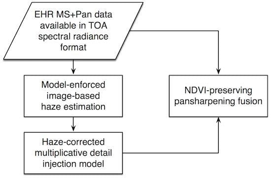
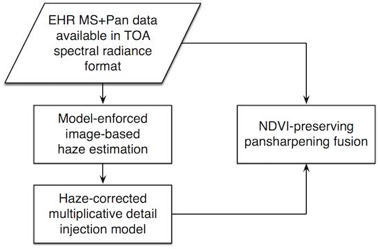
5. Contrast-Based Fusion with Haze Removal

In this section, path radiance correction is introduced in (9) and (12) in order to produce estimates of low spatial resolution spectral reflectance, which is the key to contrast-based pansharpening. For this purpose, both the MS and Pan bands must be preliminarily de-hazed. While the haze of narrow spectral bands can be calculated through either model-based or image-based techniques [35], calculation of the haze of a broad band is less immediate, because phenomena typical of narrow wavelength intervals, e.g., scattering and absorption, are spread over a large interval and thus less easily quantifiable. A viable solution consists of inferring the haze of Pan by means of the haze values of individual narrow bands that have been previously calculated. From (5), since the path radiance is assumed to be spatially uniform within a scene of moderate size and the LS residue, ϵ , exhibits minimum mean square error (MSE) and hence zero mean, the path radiances of I ^ L , of P L and, trivially, of P , are identical. The former can be easily calculated from the set of MMSE spectral weights, w ^ k , and the set of estimated path radiances, L P ( k ) ,
L P ( P ) = L P ( P L ) = L P ( I ^ L ) = w ^ 0 + k w ^ k · L P ( k ) .
After de-hazing of all the bands, including Pan, histogram matching is to be accomplished from de-hazed data. It is noteworthy that the goal of histogram matching is different for CS and MRA fusion. In the former case: (a) the mean of Pan is forced to be identical to the mean of the intensity component, in order to avoid injecting spatial details having nonzero mean; (b) the standard deviation of P L is forced to be identical to that of I L , to avoid over-/under-enhancement. For MRA fusion, equalization of the mean of Pan to that of M ^ k was introduced in [22] to perform an implicit adjustment of haze between MS and Pan. In the present case, in which such an adjustment is explicitly performed, only equalization of the MS-to-Pan gains should be accomplished.
Upon these premises, from the general model of contrast-based CS fusion (9), the atmospheric model inversion (15) and the path radiances of the broad bands (18), the haze-corrected version is given by:
M ^ k = ( M ˜ k L P ( k ) ) · P L P ( I ^ L ) I ^ L L P ( I ^ L ) + L P ( k ) , k = 1 , , N .
With simple manipulations, (19) can be written as an addition of spatial details driven by a space-varying multiplicative gain that is proportional to the k-th de-hazed band:
M ^ k = M ˜ k + M ˜ k L P ( k ) I ^ L L P ( I ^ L ) · ( P I ^ L ) , k = 1 , , N .
Starting from the general model of contrast-based MRA fusion (12), the haze-corrected version is given by:
M ^ k = ( M ˜ k L P ( k ) ) · P L P ( I ^ L ) P L L P ( I ^ L ) + L P ( k ) , k = 1 , , N .
Note that in (21), the histogram matching gain factors of Pan (11), σ M ˜ k / σ P L , do not explicitly appear because they cancel each other in the ratio. Analogously to (20), the additive version of (21) can be stated as:
M ^ k = M ˜ k + M ˜ k L P ( k ) P L L P ( I ^ L ) · ( P P L ) , k = 1 , , N .
Equations (19) and (21) may be easily explained by watching (15), in which the radiative transfer model is inverted to yield the surface reflectance product. Accordingly, the reflectance is given by the spectral radiance diminished by the path-radiance (offset) divided by the product of the upward atmospheric transmittance by the total solar irradiance. The rationale is that the de-hazed Pan image viewed by the satellite is proportional to the product of the solar irradiance (that generated it) by the upward transmittance (that determined its crossing of the atmosphere). Histogram matching to the k-th band adjusts the broadband Pan/intensity in such a way that it matches the product of narrowband irradiance by upward transmittance. Once a map of low spatial resolution spectral reflectance is obtained, it is sharpened by multiplying its pixels by something that is proportional to the high spatial resolution irradiance multiplied by the upward transmittance, that is either Pan histogram matched to the MMSE intensity or Pan histogram matched to the de-hazed k-th interpolated MS band.
As an example of the accurate spectral preservation of the haze-corrected pansharpening, let us calculate NDVI from the pansharpened red and NIR bands. Denote with R ˜ and N ˜ the interpolated red and NIR bands and with R ^ and N ^ their pansharpened versions. Then, (17) written for de-hazed pansharpened spectral radiance values, e.g., MRA (21), yields:
NDVI = α · ( N ^ L P ( N ˜ ) ) ( R ^ L P ( R ˜ ) ) α · ( N ^ L P ( N ˜ ) ) + ( R ^ L P ( R ˜ ) ) = α · ( N ˜ L P ( N ˜ ) ) · P L P ( I ^ L ) P L L P ( I ^ L ) ( R ˜ L P ( R ˜ ) ) · P L P ( I ^ L ) P L L P ( I ^ L ) α · ( N ˜ L P ( N ˜ ) ) · P L P ( I ^ L ) P L L P ( I ^ L ) + ( R ˜ L P ( R ˜ ) ) · P L P ( I ^ L ) P L L P ( I ^ L ) = α · ( N ˜ L P ( N ˜ ) ) ( R ˜ L P ( R ˜ ) ) α · ( N ˜ L P ( N ˜ ) ) + ( R ˜ L P ( R ˜ ) ) .
The proof is analogous for CS pansharpening (19). Thus, contrast-based pansharpening, either CS or MRA, with haze correction is capable of thoroughly preserving the NDVI of the original (interpolated) MS data. This is not surprising because NDVI depends on the reflectance, and a correct pansharpening cannot increase the spatial resolution of the original reflectance, but simply enhances the geometrical information of the scene without increasing the associated color information. On the contrary, Equation (24), as well as independent recent studies [49] state that if the contrast-based fusion model is not haze-corrected or, worse, if the red and NIR bands are not properly de-hazed before calculating the NDVI, an unlikely high-frequency spatial pattern will appear in the NDVI map calculated from pansharpened data.

6. Experimental Results

6.1. Methods

Path-radiance correction (PRC) has been considered for two optimized contrast-based methods, one relying on CS, the another on MRA [11]. The two methods with path-radiance correction are labeled as CSw/PRC (20) and MRAw/PRC (22). The two versions without path-radiance correction, CSw/oPRC and MRAw/oPRC, are given by (9) with MMSE intensity (5) and by (12), respectively. All spatial filters are separable Gaussian with the amplitude at Nyquist equal to 0.25 [9]. To allow for homogeneous comparisons, interpolation of MS data to yield M ˜ k is performed in two steps by means of the 23-taps filter described in [50], which is suitable for 1:2 interpolation. The method labeled as Expdenotes plain interpolation without injection of details.

6.2. Dataset

Two GeoEye-1 observations of the same scene have been acquired on the area of Collazzone, a small town in Central Italy, on different dates of the same year, that is on 27 May 2010 and 13 July 2010. The spatial sampling interval (SSI) is 2 m for MS (blue, green, red and NIR bands) and 0.5 m for Pan, respectively. The DNs of the 11-bit fixed-point representation are proportional to spectral radiances through a set of floating-point calibration gains (metadata). All offsets are equal to zero. The choice of the sensor is motivated by the compatibility of the traditional R, G, B and NIR bands with the corresponding bands of WorldView-2/3/4, which, in turn, exhibit four additional bands, two of which lie outside the span of the Pan band.
The area investigated in the following is approximately 1 km 2 (2048 × 2048 Pan and 512 × 512 MS). All the images have been orthonormalized by using a digital terrain model (DTM) available at a 10-m resolution for all spatial coordinates. In particular, the second dataset (slave) has been coregistered on the first one (master). The lack of a digital surface model (DSM) including also buildings and man-made structures in general is not crucial for the analysis of vegetation, because residual misregistrations (Pan-to-MS and date-to-date) are confined in the urban area. Figure 2 shows 2048 × 2048 close-ups of the panchromatic images acquired on May (Figure 2a) and July (Figure 2b). Figure 3 shows the 512 × 512 MS images, resampled to the Pan scale, for the two dates, both in true (3-2-1) and false (4-3-2) color compositions.

6.3. Assessments

Quality evaluations have been carried out at the full spatial scale (0.50 m for GeoEye-1 products) equal to that of the original Pan [51,52]. The check at full scale foresees separate measurement of spectral consistency, which may be defined according to Wald’s protocol [53], and spatial consistency, which may be defined according to either QNR [54] or Khan’s [55] protocol. Spectral consistency is the complement of the normalized spectral distortion that is defined as D λ according to the QNR protocol or D λ ( K ) according to Khan’s protocol. Analogously, spatial consistency is defined as the complement of the normalized spatial distortion, either D S or D S ( K ) , respectively. The spectral consistency of Khan’s protocol strictly implements the guidelines of Wald’s consistency property. The crossed coupling of the QNR and Khan’s protocols is preferable, and a global index, referred to as hybrid QNR (HQNR), was recently introduced and validated [56]:
HQNR 1 D λ ( K ) · 1 D S .

6.4. Estimation of Path Radiances

The haze-corrected versions of CS (20) and MRA (22) require one value of path radiance estimated for each band. In principle, also image-based methods are feasible because band offset metadata in the file header are all identically zero. In this case, the path-radiance values estimated for each band will not be expressed in physical units, but as DNs. Conversion to spectral radiance units, typically (W·m 2 · sr 1 · μ m 1 ) or (mW·cm 2 · sr 1 · μ m 1 ) requires subsequent multiplication by the calibration gain metadata.
The path radiance is arguably a fraction of the minimum of spectral radiance attained over the scene. If the scene is large enough and hence statistically consistent, setting the actual minimum equal to the first-percentile of the histogram ensures robustness to the photon and thermal instrument noise [57], appearing as fluctuations of the dark signal around its average, and to outliers originated by pattern-gain correction of the instrument. The rationale is that the minimum attained over a certain spectral band generally depends on the spatial scale of representation, whereas the path radiance does not, at least for a wide range of metric or sub-metric scales. Invariance to scales between 2 m and 8 m is attained with p-tile values between 0.5 and one. Below 0.5, the invariance is weak; above one, the invariance is almost perfect. Thus, the path radiance of the B band, which is usually approximated by the minimum over the scene [34], may be approximated by one p-tile.
Once the path-radiance of the blue channel, L P (B), is known, the intercept of the G-to-(B– L P (B)) scatterplot yields an estimate of L P (G); analogously for the R channel, L P (R) may be estimated from the R-to-(G– L P (G)) scatterplot. This empirical/statistical approach holds for the visible bands [35]. For calculating the path radiance of NIR, which is practically uncorrelated with the visible bands [58] in the presence of vegetation, the scatterplot method may fail, unless its calculation, either supervised or unsupervised, e.g., NDVI-enforced, is performed on non-vegetated areas. Otherwise, a reasonable physical approximation is that the L P of NIR is set equal to zero.
Furthermore, a modeling of the atmosphere was considered. In this case, the DNs must be preliminarily calibrated my means of the gain metadata. The Fu–Liou–Gu (FLG) radiative transfer model [36] requires acquisition year, month, day, local time, longitude, latitude and possibly the type of landscape for setting aerosols [59,60] (advected [61,62] or local) both in the boundary layer [63,64] or upper troposphere. The content of water vapor may be inferred from the presence of cirrus clouds in the visible bands [65,66]. Such a model directly yields values of path radiance in predefined bands, roughly corresponding to those of MS scanners, like Landsat 8 OLI. With small adjustments to fit the R and NIR bands of GeoEye-1, it was found that the modeled path radiance is well approximated by 95% of the one p-tile of B, 65% of the one p-tile of G, 45% of the one p-tile of R and 5% of the one p-tile of NIR. Path-radiance values are correlated to one another: for a clear atmosphere dominated by Rayleigh scattering, the path radiance is inversely proportional to the fourth power of the wavelength.
The results reported in Section 6.5 are the best attainable varying with the estimated path radiances. An exhaustive search at steps of one DN was performed for each dataset: the optimal path radiances are those that optimize with-reference fusion scores, on average, at the degraded spatial scale, i.e., when the ground truth is available as a reference. With FLG-modeled path radiances and model-enforced image-based path-radiances, the performance is about 0.1% lower than that achieved with the exhaustive search. Therefore: (i) the radiative transfer model actually rules the performance of contrast-based MS pansharpening; (ii) the accuracy of path radiance estimation is not crucial, at least for clear atmospheres.

6.5. Fusion Simulations

The GeoEye-1 pansharpened images at a 0.5-m scale are portrayed in Figure 4 and Figure 5, for true and false color display. What immediately stands out is that the synthesis of vegetated areas is much more realistic and accurate for the haze-corrected methods. This is mostly noticeable in the true color display, the bands of which are more largely affected by haze compared to those of the false color. Without correction, the texture of the canopies, which appears in Pan, originating from the red-edge and NIR wavelengths, but would be much less noticeable in the bands covering the visible spectrum, is transplanted in the fusion products and originates an unlikely over-enhancement, marred by a blueish texture. In fact, the blue band exhibits the largest path radiance over the visible spectrum. The visual quality of non-vegetated areas is generally good for all methods. While the difference between corrected and non-corrected methods stands out, especially in the true color display, the difference between the CS and MRA approaches, both with or without correction, is not perceivable.
Table 1 reports the scores achieved by the two CS and MRA contrast-based methods, with and without path-radiance correction. The baseline GS spectral sharpening and the optimized BDSD [38], practically unsurpassed for pansharpening of four-band MS images [8], are also included for benchmarking. The interpolated low-resolution MS is included in the comparison as Exp. The benefits of the path-radiance correction are evaluated in terms of the decrement in both spectral and spatial distortions, as measured according to the QNR [54] ( D λ , D S ) and Khan’s [55] ( D λ ( K ) , D S ( K ) ) protocol. For the QNR protocol, both distortions are approximately halved thanks to the haze-corrected injection. For Khan’s protocol, the spectral distortions benefit by a 20–25% reduction from the correction, while the spatial distortion almost doubles in size with the correction. A match with visual quality suggests that the spatial distortion of QNR and Khan’s spectral distortion should be coupled together to yield a global quality index (24). The QNR and Khan’s quality indexes are reported together with HQNR in the last three columns of Table 1. QNR detects a high improvement of the corrected versions, both CS and MRA, over the uncorrected ones. The global index of Khan’s protocol is extremely flat, almost insensitive to the haze-correction detail injection. However, the unfused image is somewhat poorer than all the fused images, and this is reasonable. The mixed index HQNR detects significant improvements of the corrected versions and places the quality of the unfused image Exp quite in the middle of the corrected and uncorrected CS/MRA. This result is consistent with the tests at degraded scale carried out in [37].
Numerical results are reported also for the second date, in which most of the vegetated fields have been cropped. The difference in performance due haze correction is approximately halved, thereby revealing that the correction is particularly effective for vegetated areas. Figure 1 shows that the red edge and part of the NIR wavelengths are captured by the bandwidth of Pan and hence are injected into the visible bands, where they originate an unlikely texture, particularly annoying in the blue band, in which the path radiance is most relevant. The removal of path radiance in the multiplicative injection model cancels the band offsets that multiply by the texture and thus makes it disappear. Whenever the bandwidth of Pan is narrow, e.g., for Landsat 8 OLI data [45], it is expected that the path-radiance correction is poorer in performance than for EHR data, in which the Pan instrument covers part of the NIR spectrum.
Eventually, NDVI was calculated from pansharpened images and found to be identical to NDVI calculated from the original interpolated MS bands, as otherwise proven in (24). While the area of the town is moderately affected by changes in the vegetation cover, the surrounding agricultural area is greatly changed after the harvest. Woods and trees in general are less affected by seasonal changes. This behavior is highlighted by the seasonal difference of NDVI shown in Figure 6, in which changes of July over May and vice versa are displayed. The conclusion is that pansharpening cannot improve the spatial resolution of NDVI, which is purely spectral information, but can impair the fidelity of the NDVI map calculated from the original data, as otherwise found in other studies [49], in which NDVI was calculated from pansharpened data in TOA spectral reflectance format. The proposed haze-corrected contrast-based detail injection model is a viable solution that thoroughly preserves the spectral information of the original MS data.

7. Conclusions

In this study, we pointed out that the step of MS path-radiance estimation and correction is the key to attain improved performance from traditional pansharpening methods based on spatial modulation. Whenever the bandwidth of Pan encompasses the MS bands, an optimized intensity component can be achieved through multivariate regression of low-pass-filtered Pan to MS, and optimal injection of spatial details can be achieved through haze removal. The path radiance of each band, L P ( k ) , is estimated, subtracted before the spatial modulation and reinserted after fusion. Both visual and numerical assessments highlight improvements, especially noticeable in the true color display of vegetated areas.
As a further result of this study, it is proven that the haze-corrected multiplicative method, either CS or MRA, identically preserves the NDVI, or any other normalized differential index, of the original MS data. The proposed haze-corrected pansharpening method is extremely fast and computationally comparable with standard methods, like Gram–Schmidt (GS) and Brovey transform (BT). The procedure may need minor adjustments, e.g., for WorldView-2/3/4 data, in which the outermost bands are not encompassed by Pan. In this case, a viable solution consists of forcing to zero the spectral weights of the outermost bands. This will be a possible hint for future investigations and developments.
References

Author Contributions

Conceptualization, L.A. and A.G.; Methodology, S.L. and G.V.; Software, A.G. and G.V.; Validation, B.A. and L.A. and A.G.; Formal Analysis, L.A. and S.L.; Investigation, L.A. and A.G.; Resources, B.A. and G.V.; Data Curation, B.A. and A.G.; Writing—Original Draft Preparation, L.A.; Writing—Review & Editing, B.A. and A.G. and S.L. and G.V.; Visualization, A.G. and S.L.; Supervision, L.A. and S.L.; Project Administration, A.G. and B.A.; Funding Acquisition, B.A.

Funding

This research was funded in part by Tuscany Region, Project SMART, in the framework of POR-FESR 20142020, for development of an advanced imaging spectrometer.

Acknowledgments

The authors are grateful to Roberto Carlà and Stefano Baronti of IFAC-CNR, for providing the GeoEye-1 datasets and for useful discussions.

Conflicts of Interest

The authors declare no conflict of interest. The funding sponsors had no role in the design of the study; in the collection, analyses, or interpretation of data; in the writing of the manuscript, and in the decision to publish the results.

References

  1. Alparone, L.; Aiazzi, B.; Baronti, S.; Garzelli, A. Remote Sensing Image Fusion; CRC Press: Boca Raton, FL, USA, 2015. [Google Scholar]
  2. Selva, M.; Aiazzi, B.; Butera, F.; Chiarantini, L.; Baronti, S. Hyper-sharpening: A first approach on SIM-GA data. IEEE J. Sel. Top. Appl. Earth Obs. Remote Sens. 2015, 8, 3008–3024. [Google Scholar] [CrossRef]
  3. Zhang, H.K.; Huang, B. A new look at image fusion methods from a Bayesian perspective. Remote Sens. 2015, 7, 6828–6861. [Google Scholar] [CrossRef]
  4. Garzelli, A. A review of image fusion algorithms based on the super-resolution paradigm. Remote Sens. 2016, 8, 797. [Google Scholar] [CrossRef]
  5. Meng, X.; Shen, H.; Li, H.; Zhang, L.; Fu, R. Review of the pansharpening methods for remote sensing images based on the idea of meta-analysis. Inf. Fusion 2019, 46, 102–113. [Google Scholar] [CrossRef]
  6. Aly, H.A.; Sharma, G. A regularized model-based optimization framework for pan-sharpening. IEEE Trans. Image Process. 2014, 23, 2596–2608. [Google Scholar] [CrossRef] [PubMed]
  7. Masi, G.; Cozzolino, D.; Verdoliva, L.; Scarpa, G. Pansharpening by convolutional neural networks. Remote Sens. 2016, 8, 594. [Google Scholar] [CrossRef]
  8. Vivone, G.; Alparone, L.; Chanussot, J.; Dalla Mura, M.; Garzelli, A.; Licciardi, G.A.; Restaino, R.; Wald, L. A critical comparison of pansharpening algorithms. In Proceedings of the IEEE IGARSS, Quebec City, QC, Canada, 13–18 July 2014; pp. 191–194. [Google Scholar]
  9. Alparone, L.; Aiazzi, B.; Baronti, S.; Garzelli, A. Spatial methods for multispectral pansharpening: Multiresolution analysis demystified. IEEE Trans. Geosci. Remote Sens. 2016, 54, 2563–2576. [Google Scholar] [CrossRef]
  10. Restaino, R.; Vivone, G.; Dalla Mura, M.; Chanussot, J. Fusion of multispectral and panchromatic images based on morphological operators. IEEE Trans. Image Process. 2016, 25, 2882–2895. [Google Scholar] [CrossRef] [PubMed]
  11. Alparone, L.; Garzelli, A.; Vivone, G. Intersensor statistical matching for pansharpening: Theoretical issues and practical solutions. IEEE Trans. Geosci. Remote Sens. 2017, 55, 4682–4695. [Google Scholar] [CrossRef]
  12. Xie, B.; Zhang, H.K.; Huang, B. Revealing implicit assumptions of the component substitution pansharpening methods. Remote Sens. 2017, 9, 443. [Google Scholar] [CrossRef]
  13. Vivone, G.; Restaino, R.; Chanussot, J. A regression-based high-pass modulation pansharpening approach. IEEE Trans. Geosci. Remote Sens. 2018, 56, 984–996. [Google Scholar] [CrossRef]
  14. Garzelli, A.; Nencini, F. Fusion of panchromatic and multispectral images by genetic algorithms. In Proceedings of the 2006 IEEE International Symposium on Geoscience and Remote Sensing Symposium, Denver, CO, USA, 31 July–4 August 2006; pp. 3810–3813. [Google Scholar]
  15. Garzelli, A.; Nencini, F. Panchromatic sharpening of remote sensing images using a multiscale Kalman filter. Pattern Recognit. 2007, 40, 3568–3577. [Google Scholar] [CrossRef]
  16. Aiazzi, B.; Baronti, S.; Selva, M.; Alparone, L. Enhanced Gram-Schmidt spectral sharpening based on multivariate regression of MS and Pan data. In Proceedings of the 2006 IEEE International Symposium on Geoscience and Remote Sensing Symposium, Denver, CO, USA, 31 July–4 August 2006; pp. 3806–3809. [Google Scholar]
  17. Aiazzi, B.; Alparone, L.; Baronti, S.; Garzelli, A.; Selva, M. MTF-tailored multiscale fusion of high-resolution MS and Pan imagery. Photogramm. Eng. Remote Sens. 2006, 72, 591–596. [Google Scholar] [CrossRef]
  18. Schowengerdt, R.A. Remote Sensing: Models and Methods for Image Processing, 2nd ed.; Academic Press: Orlando, FL, USA, 1997. [Google Scholar]
  19. Gillespie, A.R.; Kahle, A.B.; Walker, R.E. Color enhancement of highly correlated images-II. Channel ratio and “Chromaticity” Transform techniques. Remote Sens. Environ. 1987, 22, 343–365. [Google Scholar] [CrossRef]
  20. Munechika, C.K.; Warnick, J.S.; Salvaggio, C.; Schott, J.R. Resolution enhancement of multispectral image data to improve classification accuracy. Photogramm. Eng. Remote Sens. 1993, 59, 67–72. [Google Scholar]
  21. Zhang, Y. A new merging methods and its spectral and spatial effects. Int. J. Remote Sens. 1999, 20, 2003–2014. [Google Scholar] [CrossRef]
  22. Liu, J.G. Smoothing filter based intensity modulation: A spectral preserve image fusion technique for improving spatial details. Int. J. Remote Sens. 2000, 21, 3461–3472. [Google Scholar] [CrossRef]
  23. Alparone, L.; Aiazzi, B.; Baronti, S.; Garzelli, A. Sharpening of very high resolution images with spectral distortion minimization. In Proceedings of the 2003 IEEE International Symposium on Geoscience and Remote Sensing Symposium, Toulouse, France, 21–25 July 2003; pp. 458–460. [Google Scholar]
  24. Aiazzi, B.; Baronti, S.; Lotti, F.; Selva, M. A comparison between global and context-adaptive pansharpening of multispectral images. IEEE Geosci. Remote Sens. Lett. 2009, 6, 302–306. [Google Scholar] [CrossRef]
  25. Garzelli, A.; Benelli, G.; Barni, M.; Magini, C. Improving wavelet-based merging of panchromatic and multispectral images by contextual information. In Image and Signal Processing for Remote Sensing VI; Serpico, S.B., Ed.; SPIE: Bellingham, WA, USA, 2001; Volume 4170, pp. 82–91. [Google Scholar]
  26. Restaino, R.; Dalla Mura, M.; Vivone, G.; Chanussot, J. Context-adaptive pansharpening based on image segmentation. IEEE Trans. Geosci. Remote Sens. 2017, 55, 753–766. [Google Scholar] [CrossRef]
  27. Vivone, G.; Restaino, R.; Dalla Mura, M.; Licciardi, G.; Chanussot, J. Contrast and error-based fusion schemes for multispectral image pansharpening. IEEE Geosci. Remote Sens. Lett. 2014, 11, 930–934. [Google Scholar] [CrossRef]
  28. Alparone, L.; Facheris, L.; Baronti, S.; Garzelli, A.; Nencini, F. Fusion of multispectral and SAR images by intensity modulation. In Proceedings of the Seventh International Conference on Information Fusion, Stockholm, Sweden, 28 June–1 July 2004; Volume 2, pp. 637–643. [Google Scholar]
  29. Pacifici, F.; Longbotham, N.; Emery, W.J. The importance of physical quantities for the analysis of multitemporal and multiangular optical very high spatial resolution images. IEEE Trans. Geosci. Remote Sens. 2014, 52, 6241–6256. [Google Scholar] [CrossRef]
  30. Jing, L.; Cheng, Q. Two improvement schemes of PAN modulation fusion methods for spectral distortion minimization. Int. J. Remote Sens. 2009, 30, 2119–2131. [Google Scholar] [CrossRef]
  31. Jing, L.; Cheng, Q. An image fusion method taking into account phenological analogies and haze. Int. J. Remote Sens. 2011, 32, 1675–1694. [Google Scholar] [CrossRef]
  32. Jing, L.; Cheng, Q. Spectral change directions of multispectral subpixels in image fusion. Int. J. Remote Sens. 2011, 32, 1695–1711. [Google Scholar] [CrossRef]
  33. Li, H.; Jing, L. Improvement of a pansharpening method taking into account haze. IEEE J. Sel. Top. Appl. Earth Obs. Remote Sens. 2017, 10, 5039–5055. [Google Scholar] [CrossRef]
  34. Chavez, P.S., Jr. An improved dark-object subtraction technique for atmospheric scattering correction of multispectral data. Remote Sens. Environ. 1988, 24, 459–479. [Google Scholar] [CrossRef]
  35. Chavez, P.S., Jr. Image-based atmospheric corrections–Revisited and improved. Photogramm. Eng. Remote Sens. 1996, 62, 1025–1036. [Google Scholar]
  36. Fu, Q.; Liou, K.N. On the correlated k-distribution method for radiative transfer in nonhomogeneous atmospheres. J. Atmos. Sci. 1992, 49, 2139–2156. [Google Scholar] [CrossRef]
  37. Lolli, S.; Alparone, L.; Garzelli, A.; Vivone, G. Haze correction for contrast-based multispectral pansharpening. IEEE Geosci. Remote Sens. Lett. 2017, 14, 2255–2259. [Google Scholar] [CrossRef]
  38. Garzelli, A.; Nencini, F.; Capobianco, L. Optimal MMSE Pan sharpening of very high resolution multispectral images. IEEE Trans. Geosci. Remote Sens. 2008, 46, 228–236. [Google Scholar] [CrossRef]
  39. Garzelli, A. Pansharpening of multispectral images based on nonlocal parameter optimization. IEEE Trans. Geosci. Remote Sens. 2015, 53, 2096–2107. [Google Scholar] [CrossRef]
  40. Aiazzi, B.; Alparone, L.; Argenti, F.; Baronti, S. Wavelet and pyramid techniques for multisensor data fusion: A performance comparison varying with scale ratios. In Image and Signal Processing for Remote Sensing V; Serpico, S.B., Ed.; SPIE: Bellingham, WA, USA, 1999; Volume 3871, pp. 251–262. [Google Scholar]
  41. Aiazzi, B.; Alparone, L.; Barducci, A.; Baronti, S.; Pippi, I. Multispectral fusion of multisensor image data by the generalized Laplacian pyramid. In Proceedings of the 1999 IEEE International Symposium on Geoscience and Remote Sensing Symposium, Hamburg, Germany, 28 June–2 July 1999; pp. 1183–1185. [Google Scholar]
  42. Garzelli, A.; Nencini, F.; Alparone, L.; Baronti, S. Multiresolution fusion of multispectral and panchromatic images through the curvelet transform. In Proceedings of the 2005 IEEE International Symposium on Geoscience and Remote Sensing Symposium, Seoul, Korea, 29 July 2005; pp. 2838–2841. [Google Scholar]
  43. Aiazzi, B.; Alparone, L.; Baronti, S.; Garzelli, A.; Selva, M. Advantages of Laplacian pyramids over “à trous” wavelet transforms. In Image and Signal Processing for Remote Sensing XVIII; Bruzzone, L., Ed.; SPIE: Bellingham, WA, USA, 2012; Volume 8537, pp. 853704-1–853704-10. [Google Scholar]
  44. Otazu, X.; González-Audícana, M.; Fors, O.; Núñez, J. Introduction of sensor spectral response into image fusion methods. Application to wavelet-based methods. IEEE Trans. Geosci. Remote Sens. 2005, 43, 2376–2385. [Google Scholar] [CrossRef] [Green Version]
  45. Zhang, H.K.; Roy, D.P. Computationally inexpensive Landsat 8 Operational Land Imager (OLI) pansharpening. Remote Sens. 2016, 8, 180. [Google Scholar] [CrossRef]
  46. Bovolo, F.; Bruzzone, L.; Capobianco, L.; Garzelli, A.; Marchesi, S.; Nencini, F. Analysis of the effects of pansharpening in change detection on VHR images. IEEE Geosci. Remote Sens. Lett. 2010, 7, 53–57. [Google Scholar] [CrossRef]
  47. Aiazzi, B.; Alparone, L.; Baronti, S.; Carlà, R.; Garzelli, A.; Santurri, L. Sensitivity of pansharpening methods to temporal and instrumental changes between multispectral and panchromatic datasets. IEEE Trans. Geosci. Remote Sens. 2017, 55, 308–319. [Google Scholar] [CrossRef]
  48. Li, Z.; Zhang, H.K.; Roy, D.P.; Yan, L.; Huang, H.; Li, J. Landsat 15-m panchromatic-assisted downscaling (LPAD) of the 30-m reflective wavelength bands to Sentinel-2 20-m resolution. Remote Sens. 2017, 9, 1–18. [Google Scholar]
  49. Johnson, B. Effects of pansharpening on vegetation indices. ISPRS Int. J. Geo-Inf. 2014, 3, 507–522. [Google Scholar] [CrossRef]
  50. Aiazzi, B.; Baronti, S.; Selva, M.; Alparone, L. Bi-cubic interpolation for shift-free pan-sharpening. ISPRS J. Photogramm. Remote Sens. 2013, 86, 65–76. [Google Scholar] [CrossRef]
  51. Aiazzi, B.; Alparone, L.; Baronti, S.; Carlà, R. Assessment of pyramid-based multisensor image data fusion. In Image and Signal Processing for Remote Sensing IV; Serpico, S.B., Ed.; SPIE: Bellingham, WA, USA, 1998; Volume 3500, pp. 237–248. [Google Scholar]
  52. Carlà, R.; Santurri, L.; Aiazzi, B.; Baronti, S. Full-scale assessment of pansharpening through polynomial fitting of multiscale measurements. IEEE Trans. Geosci. Remote Sens. 2015, 53, 6344–6355. [Google Scholar] [CrossRef]
  53. Palsson, F.; Sveinsson, J.R.; Ulfarsson, M.O. A new pansharpening algorithm based on total variation. IEEE Geosci. Remote Sens. Lett. 2014, 11, 318–322. [Google Scholar] [CrossRef]
  54. Alparone, L.; Aiazzi, B.; Baronti, S.; Garzelli, A.; Nencini, F.; Selva, M. Multispectral and panchromatic data fusion assessment without reference. Photogramm. Eng. Remote Sens. 2008, 74, 193–200. [Google Scholar] [CrossRef]
  55. Khan, M.M.; Alparone, L.; Chanussot, J. Pansharpening quality assessment using the modulation transfer functions of instruments. IEEE Trans. Geosci. Remote Sens. 2009, 47, 3880–3891. [Google Scholar] [CrossRef]
  56. Aiazzi, B.; Alparone, L.; Baronti, S.; Carlà, R.; Garzelli, A.; Santurri, L. Full scale assessment of pansharpening methods and data products. In Image and Signal Processing for Remote Sensing XX; Bruzzone, L., Ed.; SPIE: Bellingham, WA, USA, 2014; Volume 9244, pp. 924402-1–924402-12. [Google Scholar]
  57. Alparone, L.; Selva, M.; Aiazzi, B.; Baronti, S.; Butera, F.; Chiarantini, L. Signal-dependent noise modelling and estimation of new-generation imaging spectrometers. In Proceedings of the 2009 First Workshop on Hyperspectral Image and Signal Processing: Evolution in Remote Sensing, Grenoble, France, 26–28 August 2009; pp. 1–4. [Google Scholar]
  58. Aiazzi, B.; Alparone, L.; Barducci, A.; Baronti, S.; Pippi, I. Estimating noise and information of multispectral imagery. Opt. Eng. 2002, 41, 656–668. [Google Scholar]
  59. Pani, S.; Wang, S.H.; Lin, N.H.; Tsay, S.C.; Lolli, S.; Chuang, M.T.; Lee, C.T.; Chantara, S.; Yu, J.Y. Assessment of aerosol optical property and radiative effect for the layer decoupling cases over the northern South China Sea during the 7-SEAS/Dongsha Experiment. J. Geophys. Res.-Atmos. 2016, 121, 4894–4906. [Google Scholar] [CrossRef]
  60. Tosca, M.; Campbell, J.; Garay, M.; Lolli, S.; Seidel, F.; Marquis, J.; Kalashnikova, O. Attributing accelerated summertime warming in thesoutheast United States to recent reductions in aerosol burden: Indications from vertically-resolved observations. Remote Sens. 2017, 9, 674. [Google Scholar] [CrossRef]
  61. Lolli, S.; Delaval, A.; Loth, C.; Garnier, A.; Flamant, P. 0.355-micrometer direct detection wind lidar under testing during a field campaign in consideration of ESA’s ADM-Aeolus mission. Atmos. Meas. Tech. 2013, 6, 3349–3358. [Google Scholar] [CrossRef] [Green Version]
  62. Campbell, J.; Ge, C.; Wang, J.; Welton, E.; Bucholtz, A.; Hyer, E.; Reid, E.; Chew, B.; Liew, S.C.; Salinas, S.; et al. Applying advanced ground-based remote sensing in the Southeast Asian maritime continent to characterize regional proficiencies in smoke transport modeling. J. Appl. Meteorol. Climatol. 2016, 55, 3–22. [Google Scholar] [CrossRef]
  63. Haeffelin, M.; Angelini, F.; Morille, Y.; Martucci, G.; Frey, S.; Gobbi, G.; Lolli, S.; O’Dowd, C.; Sauvage, L.; Xueref-Rémy, I.; et al. Evaluation of mixing-height retrievals from automatic profiling lidars and ceilometers in view of future integrated networks in Europe. Bound.-Lay. Meteorol. 2012, 143, 49–75. [Google Scholar] [CrossRef]
  64. Milroy, C.; Martucci, G.; Lolli, S.; Loaec, S.; Sauvage, L.; Xueref-Remy, I.; Lavrič, J.; Ciais, P.; Feist, D.; Biavati, G.; et al. An assessment of pseudo-operational ground-based light detection and ranging sensors to determine the boundary-layer structure in the coastal atmosphere. Adv. Meteorol. 2012, 2012, 929080. [Google Scholar] [CrossRef] [Green Version]
  65. Campbell, J.; Lolli, S.; Lewis, J.; Gu, Y.; Welton, E. Daytime cirrus cloud top-of-the-atmosphere radiative forcing properties at a midlatitude site and their global consequences. J. Appl. Meteorol. Climatol. 2016, 55, 1667–1679. [Google Scholar] [CrossRef]
  66. Lolli, S.; Madonna, F.; Rosoldi, M.; Campbell, J.R.; Welton, E.J.; Lewis, J.R.; Gu, Y.; Pappalardo, G. Impact of varying lidar measurement and data processing techniques in evaluating cirrus cloud and aerosol direct radiative effects. Atmos. Meas. Tech. 2018, 11, 1639–1651. [Google Scholar] [CrossRef] [Green Version]
Figure 1. Spectral responsivity functions of GeoEye-1 (four-bands MS + Pan). Notice that the bandwidth of Pan encompasses part of the wavelengths of the rightmost NIR band and the red edge around 730 nm.
Remotesensing 10 01308 g001
Figure 2. The 2048 × 2048 details of the GeoEye-1 Pan images taken on (a) 27 May 2010, (b) 13 July 2010.
Remotesensing 10 01308 g002
Figure 3. The 512 × 512 details of the original GeoEye-1 MS images acquired on (a,c) 27 May 2010 and (b,d) 13 July 2010. (a,b) 3-2-1 true color display; (c,d) 4-3-2 false color composite display.
Remotesensing 10 01308 g003
Figure 4. True color compositions of 256 × 256 fragments of the GeoEye-1 pansharpened images acquired (ad) on 27 May 2010 and (eh) on 13 July 2010. (a,e) component substitution without path-radiance correction (CSw/oPRC); (b,f) CSw/PRC; (c,g) multiresolution analysis without PRC (MRAw/oPRC); (d,h) MRAw/PRC.
Remotesensing 10 01308 g004
Figure 5. False color compositions (4-3-2 as R-G-B) of 256 × 256 fragments of the GeoEye-1 pansharpened images acquired (ad) on 27 May 2010 and (eh) on 13 July 2010. (a,e) CSw/oPRC; (b,f) CSw/PRC; (c,g) MRAw/oPRC; (d,h) MRAw/PRC.
Remotesensing 10 01308 g005
Figure 6. Normalized differential vegetation index (NDVI) of pansharpened images on 27 May 2010 and 13 July 2010. Map of differences in NDVI values: (left) July-to-May; (right) May-to-July.
Remotesensing 10 01308 g006
Table 1. Full-scale spectral/spatial distortion indexes and cumulative scores. GS stands for Gram–Schmidt spectral sharpening (see [16]) and BDSD for band-dependent spatial detail [38].
27-May-2010 D λ D λ ( K ) D S D S ( K ) QNRQNR ( K ) HQNR
EXP0.00000.03760.11600.05350.88400.91090.8507
CSw/oPRC0.10330.06000.14710.01400.76480.92680.8017
CSw/PRC0.05070.04670.06740.02090.88530.93340.8890
MRAw/oPRC0.10430.04450.15140.01260.76010.94340.8109
MRAw/PRC0.05230.03790.06660.02120.88460.94180.8981
GS0.06210.12350.05920.02290.88230.85640.8246
BDSD0.03260.05210.05380.01560.91540.93310.8970
13-July-2010 D λ D λ ( K ) D S D S ( K ) QNRQNR ( K ) HQNR
EXP0.00000.03020.16730.08160.83270.89070.8076
CSw/oPRC0.09620.04250.10440.01280.80950.94530.8576
CSw/PRC0.04270.03480.05800.02420.90170.94190.9092
MRAw/oPRC0.09230.03150.09390.01270.82240.95620.8776
MRAw/PRC0.04170.02820.05540.02530.90520.94720.9180
GS0.04520.09320.07390.01880.88430.88970.8399
BDSD0.01920.04110.02750.02060.95380.93910.9325

