Monitoring of Thermal Activity at the Hatchobaru–Otake Geothermal Area in Japan Using Multi-Source Satellite Images—With Comparisons of Methods, and Solar and Seasonal Effects

Abstract

The Hatchobaru–Otake (HO) geothermal field is proximal to the Kuju volcano on Kyushu, Japan. There are currently three geothermal power plants operating within this geothermal field. Herein, we explore the thermal status of the HO geothermal area using ASTER thermal infrared data to monitor heat losses from 2009 to 2017. We assessed the solar effects and seasonal variation on heat losses based on day- and night-time Landsat thermal infrared images, and compared three conventional methods of land surface temperature (LST) measurements. The normalized difference vegetation index threshold method of emissivity, the split window algorithm for LST, and the Stefan–Boltzmann equation for radiative heat flux (RHF) were used to determine the heat loss within the study area. The radiative heat loss (RHL) was 0.36 MW, 38.61 MW, and 29.14 MW in 2009, 2013, and 2017, respectively, from the HO geothermal field. The highest anomaly in RHF was recorded in 2013, while the lowest was in 2009. The RHLs were higher from Otake than from the Hatchobaru thermal area in the year of 2013 (~31%) and 2017 (~78%). The seasonal variation in the RHLs based on all three LST estimation methods had a similar pattern, with the highest RHL (about 383–451 MW) in spring and the lowest (about 10–222 MW) in autumn for the daytime images from the HO geothermal field. In the nighttime images, the highest RHL was about 35–67 MW in autumn and the lowest was about 1–3 MW in spring, based on the three LST methods for RHFs. The highest RHL was about 35–42 MW in spring (day) and 3–7 MW in autumn (night) from the Hatchobaru thermal area, analyzed separately. Similarly, the highest RHL was about 22–25 MW in spring (day) and 4–5 MW in winter (night) from the Otake thermal area. The seasonal variation was greatly influenced by the regional ambient temperature. We also observed that clouds had a huge effect, with the highest values for both LST and RHF recorded below clouds on an autumn day. Overall, we obtained higher LSTs at nighttime and lower LSTs during the day from the improved mono-window algorithm than the split window algorithms for all of the seasons. The heat losses were also higher for the improved mono-window algorithm than the split window algorithms, based on the LST nighttime thermal infrared data. Considering the error level of the LST methods and Landsat 8 band 11, this study recommends the IWM method for LST using the Landsat 8 band 10 data. This study also suggests that both the nighttime ASTER and Landsat 8 thermal infrared data could be effective for monitoring the thermal status of the HO geothermal area, given that data is available for the entire period.

1. Introduction

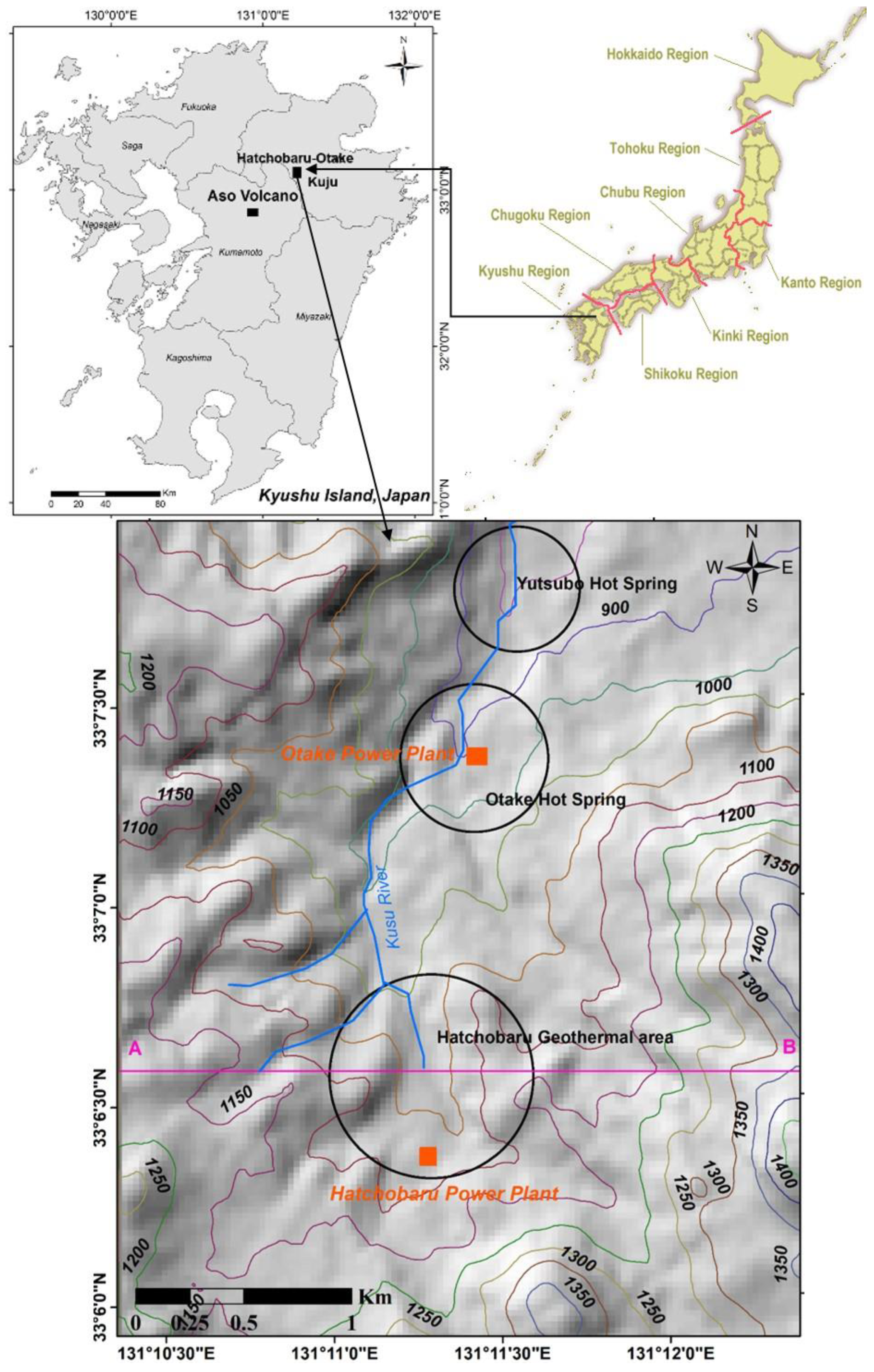
The Hatchobaru–Otake (HO) geothermal area is situated 5–6 km west of the Kuju volcano, within the Hohi graben system (the Beppu-Shimabara Graben) of central Kyushu, Japan (Figure 1) [1,2,3]. It is about 900 to 1000 m above sea level and forms a basin-like topography, surrounded by volcanic domes [4]. The extent of the HO geothermal area is about 1 km from east to west and about 3 km from north to south [5]. The Kusu River runs towards the north, through the central part of the geothermal area, and active fumaroles and hot springs are found on the eastern side of the river [4,5]. The HO geothermal area is a typical water-dominated geothermal system, which supplies steam to two geothermal power plants, Otake and Hatchobaru, installed in 1967 and 1977, respectively [6]. The Otake power plant in the Otake hot spring region has generated about 12.5 MW of peak power since 1967. 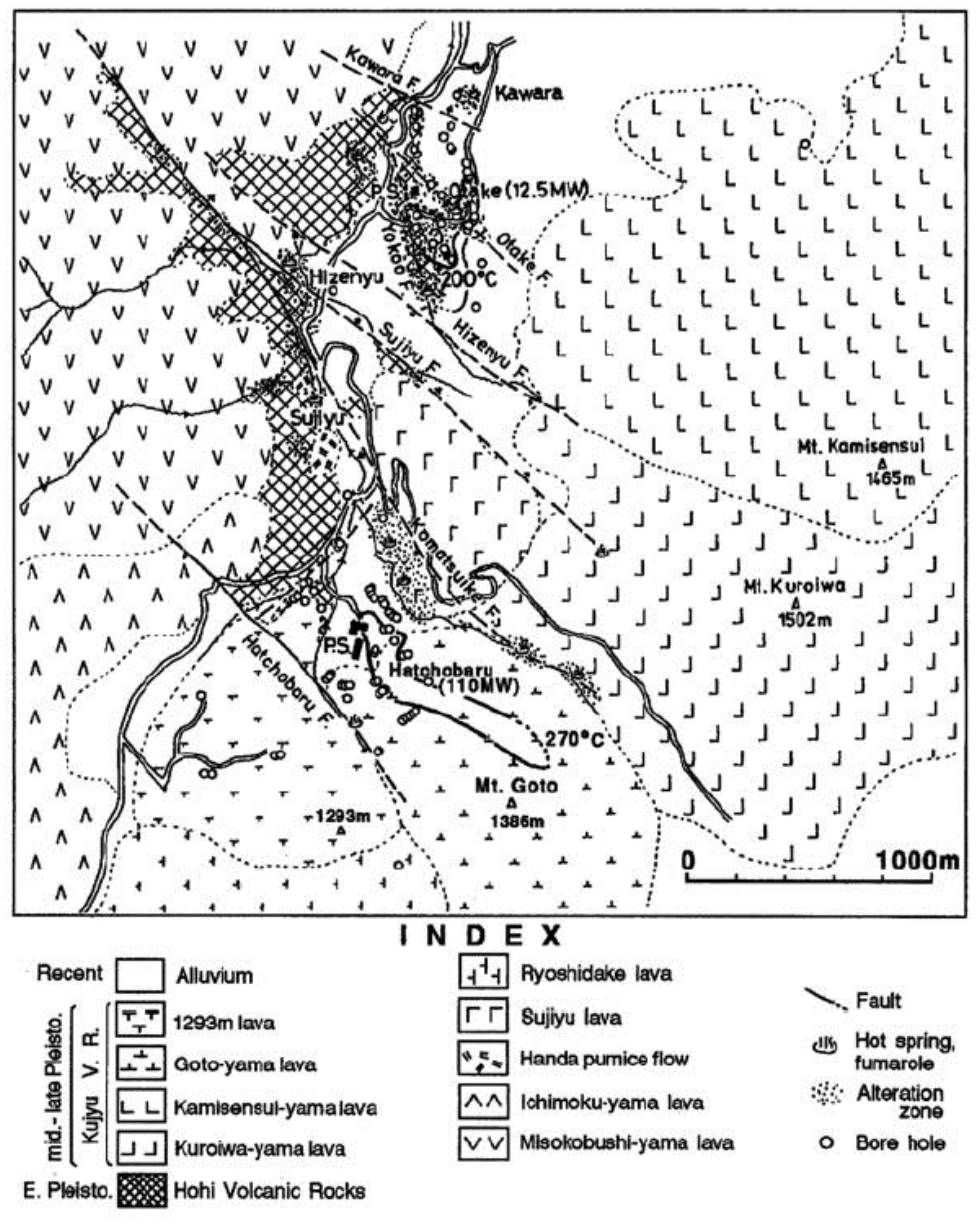Two power plants were installed in the Hatchobaru geothermal field, Unit 1 has generated about 55 MW of peak power since 1977, while Unit 2 has generated about 55 MW since 1990 [7]. The geothermal reservoirs lie about 500–1000 m below ground, along faults. The fluid temperatures are about 220–260 °C and 250–290 °C in Otake and Hatchobaru geothermal reservoirs, respectively [7,8].

Geothermal energy is one of the most important clean and renewable energies in the world. Geothermal resources are related to volcanoes or hot springs. Given their geological setting, continuous monitoring is required in order to evaluate the sustainability of the geothermal system. Typically, there are many ground-based geophysical and geochemical monitoring systems in and around geothermal power plants. Such monitoring is expensive, time-consuming, and sometimes difficult to carry out, because these areas may be within national parks and may be restricted because of fumaroles or unstable regions. Remote sensing could be used effectively for monitoring developed geothermal systems, such as the HO geothermal area in Japan; this would involve less time and money. Because the HO geothermal region is monitored using ground-based geophysical and geochemical methods, there has been no monitoring of the thermal activity of the HO area using satellite remote sensing thermal infrared data to date.

Satellite remote sensing has already been used for monitoring heat loss from active volcanoes and other geothermal areas [9,10,11,12,13,14,15]. It is very important to quantify surface heat loss from geothermal areas, in order to protect them as resources and to protect their surrounding environments. Such data can be used as an input for reservoir simulation modeling and to improve the sustainability of geothermal fluid use [16,17]. Multi-spectral satellite images, such as Landsat 8 and ASTER, have thermal bands that are used to estimate thermal anomalies, as well the heat loss from volcanic and geothermal systems. There are some limitations to using satellite images, including their coarse resolution (i.e., 30–90 m), difficulty in obtaining good-quality cloud-free images, and limited ground validation. An ASTER image has five multispectral thermal bands with a 90 m resolution (30 m resampled resolution), reflecting an electromagnetic (EM) range from 8.125 to 11.65 μm. Of these, band 13 (EM = 10.25–10.95 μm) and band 14 (EM = 10.95–11.65 μm) are used in split-window (SW) algorithms for determining the land surface temperature (LST) [18]. Subsequently, these LST estimates are used for heat loss or thermal anomaly mapping of volcanic or geothermal areas. Similarly, the Landsat 8 thermal infrared sensor (TIRS) has two thermal bands with a 100 m resolution (30 m resampled resolution). Band 10 (EM = 10.60–11.19 μm) and band 11 (EM = 11.50–12.51 μm) are used for the LST measurement of thermal anomalies using both mono-window (MW) and SW algorithms [19,20,21]. The sensor variation is distinct in the case of ASTER and Landsat 8 TIRS, as are their EM ranges of the thermal infrared data. Although there are various methods of LST measurement, no study has yet investigated the variation related to using various LST estimation methods in volcanic or geothermal regions.

Many factors affect the measurement of LST. Of them, seasonal variation could be an important factor affecting the monitoring of LST and the heat loss from thermally active areas using satellite thermal infrared (TIR) data. There are some man-made features, including buildings, roads, and cultivated fields, that will have an effect on the total geothermal RHL measurements if these features may radiate above background RHL. Another important factor to consider is meteorology. We used various meteorological data, such as the daytime versus nighttime ambient temperature and the relative humidity, so as to estimate the atmospheric transmissivity of the geothermal area during the satellite image acquisition. Solar effects are an important drawback of evaluating geothermal heat loss in daytime satellite thermal infrared data. We evaluated whether nighttime satellite thermal images could be used to avoid solar effects.

There are three pathways of heat transfer from a geothermal system, convection, conduction, and radiation. Of them, only the radiative part of heat loss can be estimated using remote sensing TIR data. The total heat loss or heat discharge rate (HDR) is the sum of the radiative, convective, and conductive heat loss from any volcanic or geothermal field. There is a relationship coefficient based on the field as well as TIR data, between the radiative heat flux (RHF) and HDR, in the literature [15,22]. We proposed, based on the total heat loss or HDR from the study area, using this relationship in the discussion. Our motivation was to evaluate the limitations and to refine the techniques of estimating heat loss using the satellite images of the HO geothermal area.

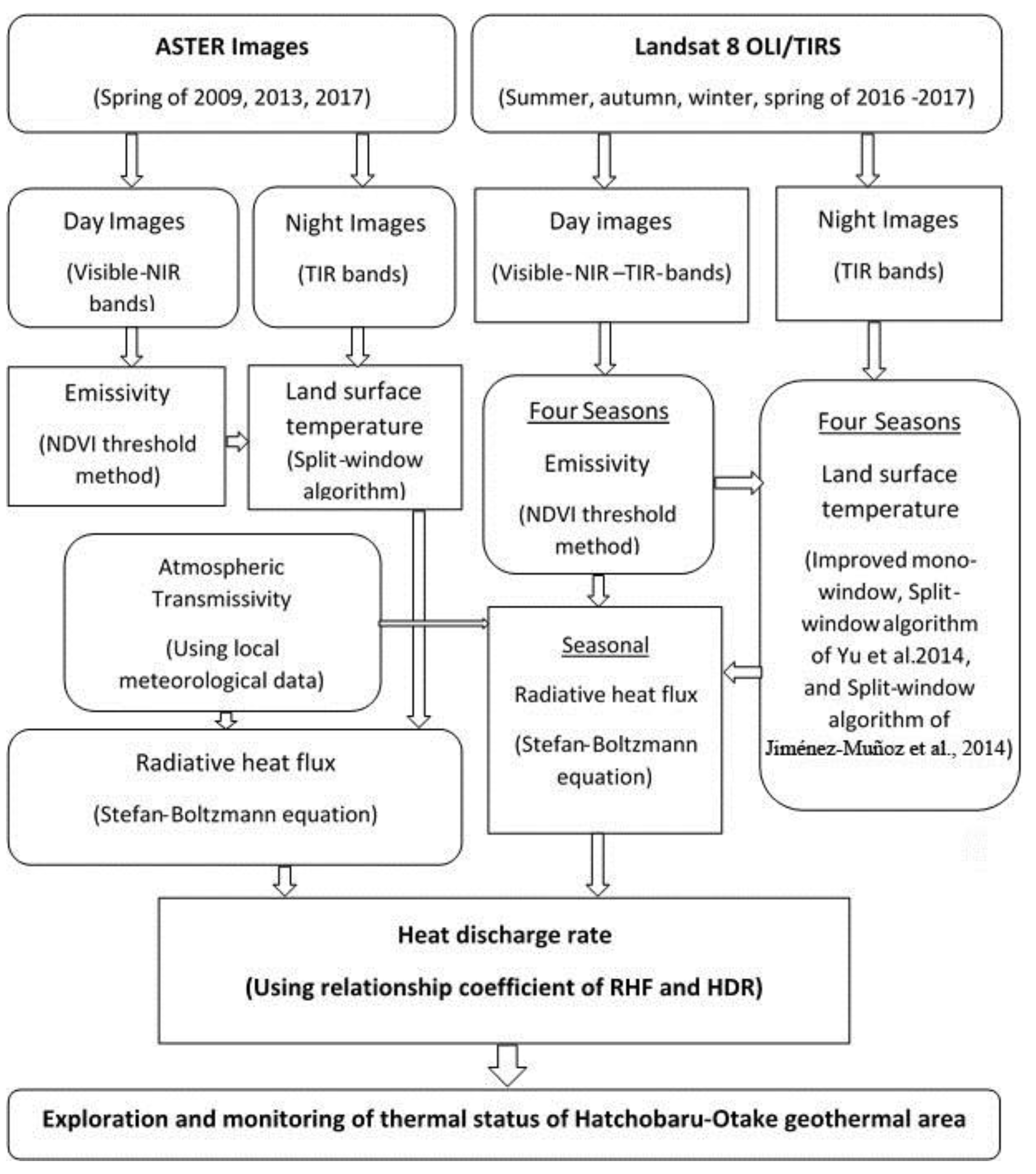
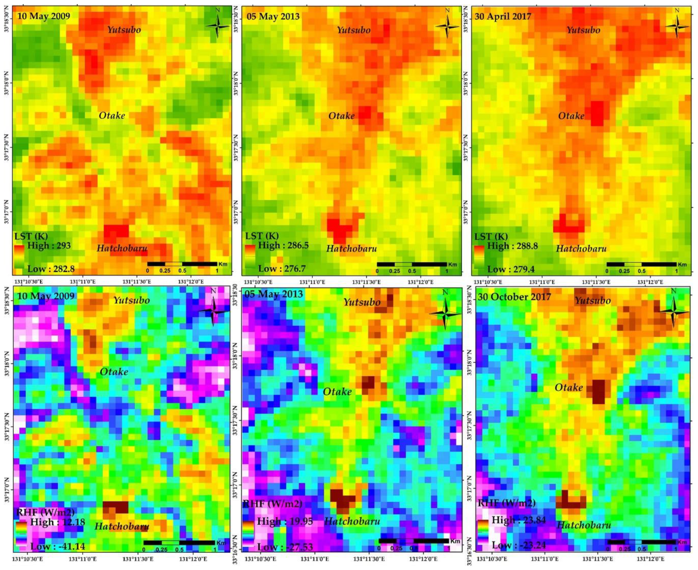
In this study, we explored and monitored the thermal status of the HO geothermal area for the first time, using satellite thermal infrared data. Our main objective was to explore its thermal anomaly using LST and to monitor its RHL from 2009 to 2017, using three sets of nighttime ASTER TIR data. A thermal anomaly means that there is a higher range of LST values in the geothermal area than in the surrounding area (i.e., LST is above ambient). The RHF anomaly indicates the RHF value above zero. Our secondary objective was to evaluate the solar and seasonal effects of heat loss using both day- and night-time Landsat 8 operational land imager (OLI)/TIRS satellite data for the study area. Lastly, there are three well-established methods for LST measurement using Landsat 8 TIR data, namely, an improved MW algorithm (IMW), the SW algorithm of Yu et al. [19], and the SW algorithm of Jiménez-Muñoz et al. [20]. We estimated the LSTs, using all of these methods to compare their variation in the heat loss estimates for the study area.

2. Geology of the Study Area

Geologically, the HO geothermal system belongs to the Hohi graben system, extending across the volcanic zone (including Aso, Kujo, and Beppu) of central Kyushu, Japan. Volcanic deposits have filled the graben system from the Miocene to Pliocene times, comprising about 2000 m of tuff, tuff breccia, sands and gravels, dense argillaceous rocks, ignimbrite, and lava flows [6]. Stratigraphically, the complex is divided into three formations—upper, intermediate, and lower—in which compacted lava layers exist in the upper and lower formations, while the intermediate one consists of tuff breccias that are fractured and highly permeable [23]. This fractured zone within the intermediate formation stores the geothermal fluids of the graben system. The surface geology comprises pyroxene-andesite lava flows and tuff breccias belonging to the Hohi volcanic rocks of the early Pleistocene age, and the hornblende-andesite lava flows of the Kuju volcanic rocks of the middle–late Pleistocene age within the HO geothermal system [24] (Figure 2). According to the literature [3], there are four groups in geological succession within the HO geothermal area, the Kuju volcanic rocks (middle–upper Pleistocene), the Hohi volcanic rocks (lower Pleistocene), the Usa Group (Miocene), and basement rocks (Palaeozoic–Mesozoic). Structurally, there are many NW-trending faults throughout the HO geothermal area, although the Hatchubaru and Komatsuike faults are the most important (Figure 2). The Komatsuike fault forms the main passage for geothermal fluids in this area, creating many thermal manifestations, such as hot springs, active fumaroles, and advanced argillic alteration along the faults [5,24] (Figure 2).

3. Materials and Methods

We used two different sets of satellite images from two different satellites in this study. One set was taken by ASTER; it was used for the exploration and monitoring of heat losses of the HO geothermal area from 2009 to 2017. The other set is from the Landsat 8 OLI/TIRS; it was used for evaluating the magnitudes of the solar effect and seasonal variation, and to compare the LST measurement methods for the Landsat 8 thermal infrared data (Figure 3). We did not take into account the ASTER image for seasonal variation, because of the unavailability of consecutive seasonal images of the study area. We used nighttime ASTER thermal band data for monitoring LST and RHL, and the daytime ASTER images for emissivity estimation within the study area. All of those images were acquired from the United States Geological Survey (USGS) archive as L1T type (i.e., level-1 and terrain corrected), which were also both radiometrically and geometrically corrected. The Landsat 8 TIRS images were available from 2013, but provided a limited number of nighttime images. We did not get required the dates, quality, and number of nighttime images for this study in the USGS archive from 2009 to 2018 for thermal status monitoring. On the other hand, three pairs of good quality day- and night-time ASTER images (same month/season’s) were available from 2009 to 2017, for the study area (

Table 1. Specifications for ASTER satellite images and local meteorological data from the Aso-san station for the study area.

Sensor of Images	Date	Day/Night	Ambient Temp. (Aso-San Station) *	Relative Humidity (Aso-San Station) *	Atmospheric Transmissivity		Altitude Adjusted Ambient Temp. (°C)
					Band 13	Band 14
ASTER	18/05/2017	Day
	30/04/2017	Night	10.7	52	0.929	0.889	10.973
	07/05/2013	Day
	05/05/2013	Night	9	73	0.917	0.87	9.273
	12/05/2009	Day
	10/05/2009	Night	17.3	35	0.928	0.888	17.573

* Data available through the Automated Meteorological Data Acquisition System in Japan.

). The ASTER pair of images from the seasons other than spring were unavailable, making seasonal comparisons with the ASTER image not possible. Hence, we acquired each season’s daytime and nighttime Landsat 8 images of the study area, covering the period from summer 2016 to spring 2017 (

Table 2. Specifications for Landsat 8 operational land imager (OLI)/thermal infrared sensor (TIRS)images and local meteorological data from the Aso-san station for the study area.

Seasons	Date	Day/Night	Ambient Temp. (°C) (Aso-San Station) *	Relative Humidity (Aso-San Station) *	Atmospheric Transmissivity		Altitude Adjusted Ambient Temp. (°C)
					Band 10	Band 11
Spring	24/04/2017	Day	12.1	50	0.92	0.874	12.373
	29/04/2017	Night	10.7	62	0.911	0.859	10.973
Winter	19/02/2017	Day	3.8	15	0.967	0.958	4.0604
	24/02/2017	Night	−3.7	78	0.949	0.924	−3.427
Autumn	30/10/2016	Day	19.1	59	0.905	0.85	12.795
	04/11/2016	Night	4.4	95	0.911	0.859	4.673
Summer	11/08/2016	Day	26.9	55	0.771	0.659	27.160
	13/06/2016	Night	16	92	0.807	0.707	16.273

* Data available through the Automated Meteorological Data Acquisition System in Japan.

). The ASTER standard products (AST_05, surface emissivity and AST_08, surface kinetic temperature) were acquired from the land processes distributed in the active archive center (LP DAAC) of USGS, so as to compare and validate the observed heat loss from the study area. The meteorological data were recorded at the Aso-san meteorological station of the Automated Meteorological Data Acquisition System (AMeDAS) in Japan. These data were adjusted for the altitude difference between the Aso-san station (1142 m above mean sea level) and the Hatchobaru power plant (1100 m above mean sea level) using the International Standard Atmosphere method (Table 1 and Table 2) [25,26]. We estimated the atmospheric transmissivity using the relative humidity, water vapour content, and ambient temperature from the Aso-san station [21,27].

3.1. ASTER Image Processing

The ASTER satellite sensor consists of three subsystems, covering the visible-infrared (VNIR), shortwave infrared (SWIR), and TIR ranges. It has three VNIR bands with a 15 m resolution, six SWIR bands with a 30 m resolution, and five TIR bands with a 90 m resolution. Initially, the daytime ASTER images were used to calculate the emissivity based on the NDVI for each land cover type, while the nighttime TIR bands were used for LST calculations, as well as for heat flux estimation and monitoring within the study area. The nighttime images were selected so as to avoid solar effects.

Land surface emissivity is very important to retrieve LST from remote sensing data. There are various approaches to predicting land surface emissivity from normalized differential vegetation index (NDVI) values [28,29]. The NDVI based emissivity retrieval method is widely used for emissivity retrieval for soil, vegetation, and water bodies [27,30]. We used the VNIR bands of the daytime ASTER images to estimate the emissivity (15 m in resolution), using the NDVI method of Qin et al. [27], based on the NDVI value for each land cover within the study area. The NDVI method was based on Equations (1) and (2) for thermal bands 13 and 14 of the ASTER data, respectively, according to the method of Qin et al [27].

ε₁₃ = A_sR_sε_s13 + A_vR_vε_v13

(1)

ε₁₄ = A_sR_sε_s14 + A_vR_vε_v14

(2)

where ε_i is the emissivity of the ASTER band (i = band13 and band 14); A_v = (1 − A_s), with A_v and A_s being the vegetation and soil coverage of any pixel; A_v = (NDVI − NDVI_s)/(NDVI_v − NDVI_s), with NDVI_v and NDVI_s being the NDVI of vegetation and soil, respectively [27]; NDVI = (b3 − b2)/(b3 + b2), in which b3 and b2 are the infrared (band 3) and red (band 2) bands of the ASTER data. The NDVI value is typically above 0.75 for the full healthy vegetation coverage for any given pixel and below 0.2 for bare ground or soil [27]. This gives R_v = 0.92762 + 0.07033A_v and R_s = 0.99782 + 0.08362A_v, where R_v and R_s are the radiance ratios of the vegetation and soil, respectively [27]. Thus, ε_s13 and ε_s14 are the spectral emissivity values of the soil for bands 13 and 14 (ε_s13 = 0.9676 and ε_s14 = 0.9779), while ε_v13 and ε_v14 are the spectral emissivity values of the vegetation for bands 13 and 14 (ε_v13 = 0.9867 and ε_v14 = 0.9899) [27].

Thermal infrared band data were used to determine the radiance values in the selected nighttime satellite images, using the metadata in Equation (3) [27]. The radiance value was used to calculate the brightness temperatures within the study area, without considering any atmospheric effects on the sensor. The brightness temperature was used to estimate the true skin temperature of the ground, using the split-window algorithm of Qin et al. [18], for the TIR band 13 and band 14 of ASTER images.

T_s = B₀ + B₁T₁₃ − B₂T₁₄

(3)

where T₁₃ and T₁₄ are the brightness temperatures of ASTER TIR band 13 and 14; B₀, B₁, and B₂ are the coefficients defined as B₀ = e₁a₁₃ − e₂a₁₄, B₁ = 1 + A + e₁b₁₃ and B₂ = A + e₂b₁₄, A = d₁₃/e₀, where a₁₃ = −60.994, b₁₃ =0.40721, a₁₄ = −63.3096, b₁₄ = 0.441977, e₁ = d₁₄ (1 − c₁₃ − d₁₃)/e₀, e₂ = d₁₃ (1 − c₁₄ − d₁₄)/e₀ and e₀ = d₁₄c₁₃ − d₁₃c₁₄; c_i = ε_iτ_i; and d_i = (1 − τ_i)(1 + [1 − ε_i]τ_i), where i represents the thermal bands of ASTER (i = band 13 and band 14), and ε_i and τ_i are the emissivity and atmospheric transmissivity of ASTER band i, respectively [27]. Here, τ₁₃ = 0.979160 − 0.062918w and τ₁₄ = 0.968144 − 0.098942w, when the water vapour content (w) is within the range of 0.4–2.0 g/cm² [27]. The total water vapour content was estimated using the relative humidity, air density, and the saturation mixing ratio from the Aso-san station [27].

The total heat loss or HDR is the sum of the conductive, convective, and radiative heat loss from the volcanoes or geothermal fields, without considering the solar effects. Given that remote sensing can only be used to determine the radiative heat loss, the ASTER thermal infrared data were used to retrieve the RHF using the Stefan–Boltzmann equation within the HO geothermal area for the period from 2009 to 2017 [10,12,31]. The RHF is defined as the radiative part of the surface heat loss (not considering solar effects) from any volcano or geothermal field. The Stefan–Boltzmann equation states that the thermal energy radiated by a true blackbody per second per unit area is proportional to the fourth power of the absolute temperature. If the hot object or geothermal system is other than an ideal radiator or blackbody, making the geothermal surface cooler than the surrounding atmosphere at temperature T_a, then the net RHF is given by the following [12,31]:

Q = σε (T_s⁴ − T_a⁴)

(4)

where Q is the RHF, σ is the Stefan–Boltzmann constant (5.6703 × 10⁻⁸ W/m² K⁴), ε is the emissivity, T_s is the surface or hot body temperature (K), and T_a is the cooler surrounding temperature (K).

The RHL was calculated by summing the pixel positive RHF values after multiplying the RHF values with the pixel area in each image of the study area. Finally, the total heat loss or HDR was proposed in the discussion section, after multiplying the total RHL by the coefficient between the RHF and HDR (6.49 or about 15%) [22].

3.2. Landsat 8 OLI-TIRS Image Processing

The Landsat 8 satellite has two sensors, an OLI and a TIRS. The OLI sensor uses nine multispectral channels to record the solar reflected images of the Earth from the visible to SWIR radiation, with a 30 m resolution, although it has a 15 m resolution in the panchromatic band. The TIRS records the surface temperatures in two longwave TIR channels of 100 m resolution (delivered as a product having a 30 m resampled resolution). The Landsat 8 OLI/TIRS satellite images for each season were processed to evaluate the seasonal variation in heat loss from the HO geothermal area. After converting the digital value of the visible-infrared bands of the daytime Landsat 8 OLI images into reflectance using metadata, the spectral emissivity values of various land covers of the study area were estimated using the NDVI threshold method, as outlined below according to the literature [19].

$${\mathsf{\epsilon }}_{\mathrm{i}}=\left\{\begin{array}{c}{\mathrm{a}}_{\mathrm{i}}{\mathrm{Q}}_{\mathrm{r}\mathrm{e}\mathrm{d}}+{\mathrm{b}}_{\mathrm{i}}\mathrm{N}\mathrm{D}\mathrm{V}\mathrm{I}<0.2\\ {\mathsf{\epsilon }}_{\mathrm{v},\mathrm{i}}{\mathrm{P}}_{\mathrm{v}}+{\mathsf{\epsilon }}_{\mathrm{s},\mathrm{i}}(1-{\mathrm{P}}_{\mathrm{v}})+{\mathrm{C}}_{\mathrm{i}}0.2\le \mathrm{N}\mathrm{D}\mathrm{V}\mathrm{I}\le 0.5\\ {\mathsf{\epsilon }}_{\mathrm{v},\mathrm{i}}+{\mathrm{C}}_{\mathrm{i}}\mathrm{N}\mathrm{D}\mathrm{V}\mathrm{I}>0.5\end{array}\right\}$$

(5)

where NDVI = (ρ_nir − ρ_r)/(ρ_nir + ρ_r), with ρ_nir and ρ_r being the reflectance of the NIR and red bands; P_v is the vegetation fraction (NDVI − NDVI_min/NDVI_max − NDVI_min)², NDVI_max = 0.5, NDVI_min = 0.2 [19]; ε_v,i is the emissivity of vegetation (TIRS band 10 = 0.9863; and band 11 = 0.9896), ε_s,i is emissivity of soil (TIRS band 10 = 0.9668; and band 11 = 0.9747) [19]; C_i is surface roughness = (1 − ε_s,i) ε_v,i F′ (1 − P_v), and F’ is the geometric factor ranging between 0 and 1 (0.55 typical) [19]. A pixel is considered as bare soil when the NDVI is less than 0.2, and the vegetation fraction, P_v, is equal to zero; in this case, the emissivity of bands 10 and 11 are ε₁₀ = 0.973 − 0.047 Q_red, and ε₁₁ = 0.984 − 0.026 Q_red, while Q_red is the reflectance of the red band of Landsat 8 OLI, ${\mathrm{a}}_{\mathrm{i}}$ and ${\mathrm{b}}_{\mathrm{i}}$ [19].

The Landsat 8 thermal band 10 and band 11 were used to estimate the LST using both the day- and night-time images of the study area in each season. We also used both the day- and night-time images to evaluate the solar effects on the LST and RHF in the geothermal area. Four established algorithms are used for the LST estimation, based on the Landsat 8 TIRS images, the MW, IMW, and two SW algorithms [18,19,20,21,32]. We evaluated the variation in heat loss from the HO geothermal area, based on the IMW and both of the SW methods of the LST estimation. At first, band 10 and band 11 of the TIR data were converted into radiance, using the following equation: L_λ = M_L × Q_cal + A_L, where L_λ is the spectral radiance (W/m² sr μm), M_L is the multiplicative scaling factor, Q_cal is the pixel value, and A_L is the radiance additive factor (based on the metadata of the image). This radiance value was converted into the effective or brightness temperature using the following equation: T_i= K₂/In(K₁/L_λ + 1), where T_i is the brightness temperature, K₁ and K₂ are thermal efficient coefficients (from the metadata of the image), and L_λ is the spectral radiance value. We used the ambient temperature and relative humidity from the Aso-san station (AMeDAS) to establish the water vapour content. Because there are difficulties involved in getting the in situ atmospheric transmissivity values for the time of the satellite pass, we used the equations of Yu et al. [19] for the atmospheric transmissivity based on water vapour content, as follows:

τ₁₀ = −0.0164w² − 0.04203w + 0.9715 (mid-latitude summer; w = 0.2 − 3.0 g/cm²),

(6)

τ₁₁ = −0.01218w² − 0.07735w + 0.9603 (mid-latitude summer; w = 0.2 − 3.0 g/cm²),

(7)

and w = (H × E × A/1000)/R_w(0)

(8)

where τ_i is the atmospheric transmissivity of the respective bands of the Landsat 8 TIRS data, w is total water vapour content (g/cm²), H is relative humidity (%), E is the saturation mixing ratio (g/kg) of the water vapour, A is air density (kg/m³), and R_w(0) = 0.6834 and 0.6356 for mid-latitude summer and winter, respectively (

Table 3. Relationships between saturation mixing ratio (E), air density (A), and air temperature (T) (after the literature [19]).

T (°C)	45	40	35	30	25	20	15	10	5	0	−5	−10
E (g.kg−1)	66.33	49.81	37.25	27.69	20.44	14.95	10.83	7.76	5.5	3.84	2.52	1.63
A (kg.m−3)	1.11	1.13	1.15	1.17	1.18	1.21	1.23	1.25	1.27	1.29	1.32	1.34

).

3.2.1. Improved Mono-Window Method

According to the IMW method of Wang et al. [21], the LSTs can be calculated using the following equation for the Landsat 8 TIRS band 10:

T_s = [c₁₀ (1 − A₁₀ − B₁₀) + (d₁₀(1 − A₁₀ − B₁₀) + A₁₀ + B₁₀) T₁₀ − B₁₀T_a]/A₁₀

(9)

where Ts is the LST derived from the Landsat 8 TIRS band 10; A₁₀ = τ₁₀ε₁₀ and B₁₀ = (1 − τ₁₀) (1 + [1 − ε₁₀] τ₁₀), where τ₁₀ is the atmospheric transmittance and ε₁₀ is the land cover emissivity for band 10 of the Landsat 8 TIRS image; T₁₀ is the brightness temperature; T_a is the effective mean atmospheric temperature obtained from the local meteorological station; and c₁₀ and d₁₀ are the coefficients for the Landsat 8 TIRS band 10.

3.2.2. Split Window Method after Yu et al.

Yu et al. [19] developed a SW algorithm based on the work of Qin et al. [30], for estimating the LST using the Landsat 8 TIRS band 10 and band 11, as follows:

T_s = T₁₀ + D₁(T₁₀ − T₁₁) + D₀

(10)

D₀ = (C₁₁[1 − A₁₀ − C₁₀] L₁₀ − C₁₀[1 − A₁₁ − C₁₁] L₁₁)/(C₁₁A₁₀ − C₁₀A₁₁)

(11)

D₁ = C₁₀/(C₁₁A₁₀ − C₁₀A₁₁)

(12)

where T_s is the LST; A_i = ε_iτ_i and C_i = (1 − τ_i) (1 + [1 − ε_i] τ_i), ε is the emissivity, τ is the atmospheric transmissivity, and L_i is the linear fitting coefficient form the literature [19].

3.2.3. Split Window Method after Jiménez-Muñoz et al.

Jiménez-Muñoz et al. [20] proposed another SW algorithm, based on Sobrino et al. [33], for the LST estimation, using Landsat 8 TIRS band 10 and band 11, as follows:

T_s = T₁₀ + c₁ (T₁₀ − T₁₁) + c₂(T₁₀ − T₁₁)² + c₀ +(c₃ + c₄w) (1 − ε) + (c₅ + c₆w) ∆ε

(13)

where Ts is the LST derived using the SW algorithm; T₁₀ and T₁₁ are the brightness temperatures of the Landsat 8 TIRS band 10 and band 11; ε is the mean of the emissivity for band 10 and band 11; ∆ε is the difference in emissivity between band 10 and 11; w is the total atmospheric water vapour content (g/cm²); and c₀ to c₆ are the SW coefficients derived from simulated data (i.e., c₀ = −0.268, c₁ = 1.378, c₂ = 0.183, c₃= 54.30, c₄ = −2.238, c₅ = −129.20, and c₆ = 16.40) [20,34].

4. Results

4.1. Monitoring Heat Loss Based on ASTER Images

Satellite images, like ASTER and Landsat 8, have previously been used to explore and monitor the thermal status of volcanoes and other geothermal areas using various techniques, including land surface temperature estimation, thermal anomaly mapping, heat loss estimation, and hydrothermal alteration mapping. With this in mind, we explored the thermal status of the HO geothermal area using both ASTER and Landsat 8 images. Specifically, we used three sets of ASTER images to determine the heat loss from 2009 to 2017. Meanwhile, the Landsat 8 OLI/TIRS images were used for comparing the methods of the LST estimation, as well as the solar and seasonal effects on heat loss within the study area. Spectral emissivity is a key component of both the LST and heat loss estimations in any geothermal or volcanic region. We used ASTER daytime images to derive the emissivity values for all of the land cover types of the study area, using NDVI thresholds. We obtained emissivity values in the range of 0.96 to 0.99 for the HO geothermal area for May of 2009, 2013, and 2017. Later, we used the NDVI values to divide the land covers into three types, bare ground or wetland areas (NDVI < 0.2), mixed cover (NDVI = 0.2–0.5), and vegetated areas (NDVI > 0.5) (Figure 4). The NDVI results showed that the bare ground or wetland areas, as well as the mixed cover, decreased slightly, while the vegetated areas increased within the study area from 2009 to 2017 (

Table 4. Summary of heat loss for the Hatchobaru–Otake geothermal area from 2009 to 2017, based on three sets of ASTER thermal infrared images. The RHL was retrieved separately for the Hatchobaru and Otake geothermal area, as indicated by the circles in Figure 1. The ambient temperature was recorded at the Aso-san station (AMEDAS) and was adjusted for variation with the altitude, using the International Standard Atmosphere method from the literature [25].

Image	Date	Day/Night	Ambient Temp. (°C)	Atmospheric Transmissivity		Landcover (sq.km)		LST (°C)			RHF (W/m2)		Hatchobaru-Otake		Hatchobaru	Otake
				Band 13	Band 14	Bared/Wetland	Mixed	Vegetated	Max	Min	Max	Min	RHL (MW)	HDR (MW)	RHL (MW)	RHL (MW)
ASTER	18 May 2017	Day				2.35	4.65	5.09
	30 April 2017	Night	10.97	0.93	0.89				17.04	5.60	31.22	−26.21	29.14	189.12	2.83	4.99
	7 May 2013	Day				2.55	5.74	3.80
	5 May 2013	Night	9.27	0.92	0.87				14.93	4.50	28.35	−23.17	38.61	250.58	3.79	5.61
	12 May 2009	Day				2.96	4.85	4.27
	10 May 2009	Night	17.57	0.93	0.89				19.98	9.40	12.98	−42.31	0.36	2.33	0.30	0.00

Notes. The total RHL was calculated after removing the RHL using the pixels with the background LST (average). LST—land surface temperature; RHF—radiative heat flux; RHL—radiative heat loss; HDR—heat discharge rate.

). In turn, LST is key to estimating heat loss in the geothermal areas. We used the SW algorithm for the LST estimation on the nighttime ASTER thermal band 13 and band 14 data for 2009, 2013, and 2017. A high LST anomaly was associated with the Hatchobaru, Otake, and Yutsubo hot spring areas in all of the years, compared with the surrounding background areas (Figure 5). The highest anomaly range (10–20 °C) was observed in 2009, while the lowest (4.5–15 °C) and intermediate (6–16 °C) values were observed in 2013 and 2017 (Figure 5). Likewise, the maximum LST value was 20 °C in 2009, and the minimum was 4.5 °C in 2013 (Table 4). The minimum image-derived LST was about 5 to 8 °C lower than the ambient temperature of the study area for all of the study years (Table 4). The average LST was higher in value than the ambient in the year of 2013 and 2017, but less in 2009 (Figure 7A).

Given that we only estimated the radiative part of the heat loss from the geothermal area using remote sensing, we used the Stefan–Boltzmann heat transfer equation to estimate the RHF of the HO geothermal area for 2009, 2013, and 2017. The highest RHF anomalies were within the geothermal area, centered on the Hatchobaru, Otake, and the Yutsubo hot spring areas (Figure 6). The maximum pixel value for RHF was 31 W/m² in 2017, 28 W/m² in 2013, and 12 W/m² in 2009 for the Hatchobaru hot spring area (Figure 6 and Table 4). The average RHF value was observed to be highest in 2013 and the lowest in 2009 (Figure 7A). The highest RHF anomaly was recorded in 2013, while the lowest was in 2009 (Figure 7C). A summation of all of the pixel positive values of RHF (after multiplied with pixel area) yielded the total RHL of the study area. The total RHL values were 0.4 MW, 38.61 MW, and 29.14 MW for 2009, 2013, and 2017 (Figure 7B). The RHLs were also estimated separately for the Hatchobaru and Otake geothermal area, considering the higher LST anomaly (Figure 5), as shown circles in Figure 1, of those geothermal areas. We obtained a comparatively low RHL (0–6 MW) for the individual geothermal areas than the whole area (0.4–39 MW), but with a similar trend of RHL (i.e., the lowest in 2009 and highest 2013) (Table 4). The RHLs were higher in value from the Otake thermal area than Hatchobaru in the year of 2013 (~31%) and 2017 (~78%). Furthermore, we calculated the relative proportion of the RHL using the pixels with the background LST (average) and geothermal LST (Figure 8). Therefore, we selected 80 random pixels’ LST values surrounding the non-geothermal area, mostly from the vegetated and mixed land covers for each image of this study, and later obtained the background LST (average) of the study area. These background LSTs (average) were used to calculate the RHL of the background region, and were then removed from the total RHL to assess the geothermal RHL. The results showed that the RHLs with a background LST (average) were significantly less than the geothermal heat loss of about 0–3% of the total RHL (Figure 8). Although this study shows that the thermal activity, measured as LST, RHF, RHL, and HDR, increased from 2009 to 2013, but declined from 2013 to 2017 within the HO geothermal area, there is uncertainty of this conclusion, due to the unavailability of each year’s ASTER images (same month/season’s) to being able to retrieve those parameters of thermal activity. This change in thermal activity affected the land cover types during the study period.

Validation of the Heat Loss with ASTER Standard Products

In this study, the nighttime ASTER standard high level products of the surface emissivity (AST_05) and the surface kinetic temperature (AST_08) were used to compare and validate the retrieved emissivity, LST, RHF, and RHL of the study area from 2009 to 2017 (Figure 9). We observed a close maximum and minimum LST, but the RHF values were a little bit less than the standard products that were observed (

Table 5. Comparison of the observed and ASTER standard products base heat loss from the study area.

Year	Observed									ASTER Standard Products *
	Emissvity (Min)	Emissvity (Max)	LST (Min) (K)	LST (Max) (K)	RHF (Min) (W/m2)	RHF (Max) (W/m2)	Hatchobaru-Otake RHL (MW)	Hatchobaru RHL (MW)	Otake RHL (MW)	Emissivity (Min)	Emissivity (Max)	LST (Min) (K)	LST (Max) (K)	RHF (Min) (W/m2)	RHF (Max) (W/m2)	Hatchobaru-Otake RHL (MW)	Hatchobaru RHL (MW)	Otake RHL (MW)
2009	0.95	0.98	282.55	293.13	−42.31	12.98	0.36	0.30	0.00	0.92	0.99	282.80	293.00	−41.14	12.18	0.18	0.18	0.00
2013	0.95	0.98	277.65	288.08	−23.17	28.35	39.70	3.79	5.61	0.93	0.99	276.70	286.50	−27.53	19.95	15.54	2.17	2.84
2017	0.95	0.98	278.75	290.19	−26.21	31.22	29.57	2.83	4.99	0.93	0.99	279.40	288.80	−23.24	23.84	25.90	2.47	4.40

* ASTER standard products, such as AST_05, surface emissivity and AST_08, and surface kinetic temperature-based results.

). This may be due to the resolution difference in the observed and standard products of 15 m and 90 m, respectively. Otherwise, we obtained a higher emissivity values range in case of the ASTER standard product than was observed (Table 5). The lowest total RHLs were obatined (about 0.18 MW) in 2009, but the highest were obtained (about 25.9 MW) in 2017, with the ASTER standard products (Table 5). We analyzed the Pearson correlation coefficient for RHL between the observed and standard products base separately for the Hatchobaru–Otake (as a whole), Hatchobaru, and Otake geothermal area, using the Pearson correlation coefficient analysis free software from the authors of [35]. We obtained strong correlation coefficints between them, that is, 0.79, 0.92, and 0.90 for the Hatchobaru–Otake (as a whole), Hatchobaru, and Otake geothermal area, respectively (Figure 10). The anomalies wre quite similar between the observed and standard products of the LST and retrieved RHF (Figure 5, Figure 6 and Figure 9). The variation of the heat loss and LST anomalies indicates the variation of the emissivity and pixel resolution between the observed and standard products base results.

4.2. Comparisons of Heat Loss Based on Methods, and Solar and Seasonal Effects Using Landsat 8 OLI/TIRS

Solar effects are one of the main drawbacks of estimating the geothermal heat loss from daytime satellite images. However, the nighttime images have no usable VNIR or SWIR bands. The Landsat 8 TIRS images have two multispectral TIR bands. Therefore, there are various methods of LST estimation for these images, based on a single band (MW algorithms) or both bands (SW algorithms). Another challenge is to obtain cloud-free good-quality satellite images of the study area in all seasons. To address such issues, we acquired very good quality daytime Landsat 8 OLI/TIRS images of the study area in all four seasons, although the autumn image had some cloud cover (Figure 11). Using only the images from the Landsat 8 OLI/TIRS sensor, we compared the heat losses during both the daytime and nighttime, in order to (i) determine the magnitude of the solar effect, (ii) evaluate variation related to using various LST derivation methods, and (iii) establish any seasonal variation. The daytime images were used to estimate the emissivity of the study area using the NDVI threshold method for the Landsat 8 images. We obtained the emissivity ranges from 0.95 to 0.99 for all of the land cover types across all of the seasons (Figure 12). The variation in emissivity depends on the land cover type, with the higher values linked to the vegetation (NDVI > 0.5), and the lower values reflecting the bare ground/wetland areas (NDVI < 0.2) or mixed cover (NDVI = 0.2 to 0.5) (Figure 11). The healthy vegetated areas had NDVI values greater than 0.5, whereas the stressed vegetation sometimes had values of the mixed class. The highest NDVI values related to the healthy vegetation were found in the summer and the lowest ones were found in winter. Meanwhile, the bare area coverage was the highest in winter and the lowest in summer, and the mixed cover was the highest in spring and autumn and the lowest in winter (Figure 13).

The LSTs were estimated using the IMW algorithm and the SW algorithms of Yu et al. [19] and Jiménez-Muñoz et al., respectively [20]. These estimates were carried out for all of the seasons within the study area using both the day- and night-time Landsat 8 TIRS images. To explore the thermal anomaly, the LSTs of all of the three methods based on the nighttime Landsat 8 TIRS data were combined as red/green/blue (RGB) false colour images. These images show the thermal anomalies within the study area. Clearly, the Hatchobaru, Otake, and Yutsubo hot spring areas had high LSTs in all of the seasons, as shown by the white pixel areas (Figure 14A–D).

Both day- and night-time Landsat 8 TIR data were used to compare the variation in the derived heat loss related to the solar effects on the daytime images. The highest LSTs were obtained proximal to the Hatchobaru, Otake, and Yutsubo hot spring areas for all of the methods and for all of the seasons, except for the autumn SW-based values during the daytime. These values were affected by cloud cover (Figure 15). The daytime LST values were the highest and the lowest in autumn. This is most likely because of the cloud effects on the TIRS data. Otherwise, summer had the highest LSTs for all three of the methods, with declining values in the spring and winter for both the maximum and minimum LSTs (Figure 19A). The nighttime LSTs estimated using the three conventional methods also identified high thermal anomalies coincident with the Hatchobaru, Otake, and Yutsubo hot spring areas (Figure 16). The maximum nighttime LSTs for all three of the methods occurred in summer, and the minimum LSTs occurred in the winter at night (Figure 19B). The highest LSTs were about 68 °C and 20 °C for day- and night-time images of the study area, respectively, although the daytime highest LST is unrealistic and resulted from the cloud coverage area (

Table 6. Seasonal variation in both the daytime and nighttime estimates of heat loss within the Hatchobaru–Otake geothermal area, based on three different methods of land surface temperature estimation from the Landsat 8 OLI/TIRS images.

Image	Season	Date	Day/Night	Landcover (Sq. Km)			LST (°C) IMW		LST (°C) SW-Yu		LST (°C) SW-Muñoz		RHF (W/m2) IWM		RHF (W/m2) SW-Yu		RHF (W/m2) SW-Muñoz		Total RHL (MW)
				Bared/Water	Mixed	Vegetated	Max	Min	Max	Min	Max	Min	Max	Min	Max	Min	Max	Min	IMW Method	SW-YU	SW-Muñoz
Landsat 8 OLI/TIRS	Spring	24 April 2017	Day	1.36	5.95	4.80	35.81	15.83	39.60	16.75	39.32	16.24	136.47	18.33	162.55	2.36	160.67	20.59	382.84	451.37	431.84
		29 April 2017	Night				13.69	6.17	14.12	5.19	13.70	5.34	14.02	−24.00	16.34	−28.79	14.16	−28.07	2.78	1.30	0.80
	Winter	19 February 2017	Day	4.66	4.81	2.64	16.26	2.74	23.95	2.00	18.23	2.74	60.95	−6.15	104.26	−9.70	72.08	−6.24	133.20	221.25	152.60
		24 February 2017	Night				2.97	−5.79	2.96	−7.96	2.62	−7.05	28.61	−10.22	28.80	−19.41	27.23	−15.56	57.14	34.01	44.44
	Autumn	30 October 2016	Day	3.19	5.90	3.03	18.38	−12.89	37.78	−24.21	68.15	−11.94	29.52	−117.15	146.10	−158.81	378.00	−113.71	9.95	156.55	222.42
		4 November 2016	Night				9.73	3.09	9.61	1.02	9.34	1.60	24.49	−7.51	24.08	−17.18	22.71	−14.51	67.26	34.92	34.14
	Summer	8 November 2016	Day	0.53	4.88	6.71	35.67	24.16	41.62	28.40	41.38	27.30	53.69	−17.88	94.17	7.52	92.57	0.87	55.91	219.89	183.99
		13 June 2016	Night				17.93	12.06	19.66	11.07	18.83	10.61	9.03	−23.34	18.73	−28.43	14.09	−30.87	1.20	5.45	1.71

Notes. The result of the daytime image of the autumn season shows unrealistic LST values (68.15 °C) due to the cloud effects of this image. The total RHLs were calculated after removing the RHL using pixels with a background LST (average). OLI/TIRS—operational land imager/thermal infrared sensor; LST—land surface temperature; RHF—radiative heat flux; RHL—radiative heat loss; IMW—improved mono-window algorithm; SW-Yu—split-window algorithm of Yu et al. [19]; and SW-Muñoz—split-window algorithm of Jiménez-Muñoz et al. [20].

).

RHF is an aspect of heat loss that is easily measured using remote sensing. The radiative heat flux (RHF) values show higher anomalies in the daytime images within the HO geothermal area in all of the seasons, except the RHFs derived using the SW-based LSTs in autumn (Figure 17). In these data, some areas show as anomalies, because of cloud cover (Figure 14). The abnormal maximum and minimum RHFs in the autumn reflect the abnormal LSTs derived when the clouds covered the daytime Landsat 8 images of the study area. Otherwise, the highest RHFs occurred in spring and lowest ones occurred in winter for all of the LST estimation methods (Figure 19C). The nighttime RHFs of the study area show positive high heat loss anomalies within the Hatchobaru, Otake, and Yutsubo hot spring areas (Figure 18). Higher positive RHF anomalies were recorded during autumn and winter than in summer and spring, reflecting their lower ambient temperatures. The ambient temperature clearly influenced the detection of heat loss at the surface, with the cooler seasonal temperatures lowering the ground temperatures and increasing the subterranean temperature gradient [17]. The maximum and minimum RHFs for all of the seasons shows similar trends for all three methods of LST estimation, but higher RHF values were obtained during winter and autumn (Figure 19D). We added all of the positive pixel values of RHF (after multiplying RHF with pixel area) in order to obtain the total RHL for both the day- and night-time seasonal TIR images. During the day, the highest total RHL occurred in spring and the lowest occurred in the autumn for all of the LST estimation methods (Figure 20A). The highest RHLs for all three of the LST estimation methods were obtained in spring, with values of 383–481 MW (Table 6). In contrast, the lowest values of 10–222 MW were measured in autumn during the day, because of the cloud coverage in this image (Figure 15 and Figure 17 and Table 6). The cloudy areas showed a higher LST compared to the surroundings. The total RHLs derived using the SW algorithm from the literature [19] were the highest in all of the seasons, except for autumn. The lowest total RHLs were derived using the IMW algorithm on the daytime images of the study area (Table 6 and Figure 20A). In the nighttime images, the total RHLs were the highest in autumn and winter with values of 34–67 MW and 34–57 MW, respectively (Table 6 and Figure 20B). In summer and spring, values of 1–6 MW and 1–3 MW, respectively, were obtained using all three LST estimation methods (Table 6). The total RHLs derived using the IMW-based LSTs had higher values than those derived using the SW-based LSTs in the nighttime images of the study area (Figure 20B). We also investigated the seasonal as well as the methods variation for both the day-and night-time RHL of the Hatchobaru and Otake thermal area separately, as shown by two circles in the thermal anomaly of Figure 14 (

Table 7. Seasonal variation in both day and night estimates of heat loss within the Hatchobaru thermal area and Otake thermal area as shown circles in Figure 13 separately based on three different methods of land surface temperature estimation from Landsat 8 OLI/TIRS images.

Time	Date	Season	Hatchobaru Thermal Area				Otake Thermal Area
			RHL (MW)			Standard Deviation	RHL (MW)			Standard Deviation
			IWM	SW-Yu	SW-Muñoz		IWM	SW-Yu	SW-Muñoz
Daytime	11 August 2016	Summer	6.52	22.86	19.02	8.54	3.82	14.44	12.15	5.59
	30 October 2016	Autumn	1.37	7.19	6.35	3.15	0.19	2.24	2.34	1.21
	19 February 2017	Winter	14.91	22.89	16.79	4.17	7.88	12.29	8.92	2.3
	24 April 2017	Spring	34.91	42.22	39.94	3.74	21.77	25.32	23.99	1.79
Nighttime	13 June 2016	Summer	0.23	0.8	0.37	0.3	0.19	0.87	0.24	0.38
	4 November 2016	Autumn	6.65	2.92	3.02	2.13	5.08	2.86	2.84	1.29
	24 February 2017	Winter	7	5.19	5.88	0.91	5.23	3.97	4.47	0.63
	29 April 2017	Spring	0.66	0.55	0.41	0.13	0.8	0.43	0.28	0.27

Notes. RHL—radiative heat loss; IMW—improved mono-window algorithm; SW-Yu—split-window algorithm of Yu et al. [19]; SW-Muñoz—split-window algorithm of Jiménez-Muñoz et al. [20].

; Figure 20C–F). In the case of the Hatchobaru thermal area, the RHLs show a similar trend of seasonal variations with the RHLs of the whole study area both in the day- and night-time, but much lesser in values such as 1–42 MW and 0.23–7 MW, respectively, in the day- and night-time (Table 7 and Figure 20C,D). On the other hand, the RHLs also showed a similar trend for seasonal variation with the whole study area in the case of the Otake thermal area (Figure 20E,F). The nighttime RHLs using all three LST methods are closely spread (standard deviation [SD] is about 0.13–0.91) for all seasons, except autumn (SD, 1.21–2.13), but the daytime RHLs are moderately spread comparatively (SD, 1.21–8.54) (Table 7). The RHLs were a little bit higher from the Hatchobaru than the Otake thermal area, independently, both in the day-and night-time (Table 7).

In addition, we calculated the relative proportion of the RHL using pixels with background LST (average) and geothermal LST on the total RHL in all four seasons, using three LST methods based RHL (Figure 21). The background LSTs (average) were computed using 80 random LST samples surrounding a non-geothermal area, mostly from vegetated and mixed land covers, for each image of this study. These background LSTs (average) were used to compute the RHL of the background and were then removed from total RHL to estimate the geothermal RHL. The results showed that RHLs with background (average) were much less than geothermal heat loss of about 0–28%, 0–4% and 0–8% of total RHL, respectively, from the retrieved RHL, based on the IMW, SW-Yu, and SW-Muñoz methods of LST (Figure 21). The background LSTs (average) were influenced mostly during the autumn and winter seasons on RHL. There were no influences from the other seasons, because the background LSTs (average) were less than or equal to the ambient, hence, the RHF values were negative or zero, according to the Stefan–Boltzmann equation for estimating RHF, in this study.

The methodological and seasonal variations in the nighttime LST and RHF values were evaluated using a 101-random point sampling of the study area (Figure 22). A high intra-seasonal variation in the LST estimation was observed with all three of the LST estimation methods. The IMW-based LSTs were higher than the estimates based on the SW algorithm, except in the summer season. Otherwise, the inter-seasonal variation in the LST values was relatively consistent, with higher LST values in summer, followed by the spring, autumn, and winter values, respectively (Figure 22). The randomly sampled RHF values based on these LST estimates also shows higher values in autumn and winter (Figure 23). To explore the differences related to the method, the point samples of the RHFs derived using all of the LST estimation methods were compared using box plot diagrams. The IMW-based LSTs had maximum values of RHF (over 20 W/m²) in both autumn and winter, with the majority of values in these seasons ranging from 5 to 20 W/m² (Figure 23A). Maximum RHFs of about 10 W/m² were recorded in the summer and spring, although the majority of random RHF samples had negative values related to the LSTs being less than ambient temperatures (Figure 23A–C). The randomly sampled RHF values based on the LSTs from one SW algorithm [19] showed higher values in the winter and lower ones in the spring (Figure 23B,C). Meanwhile, the highest RHF values in the winter were derived using the other SW algorithm [20], with the lowest values in spring (Figure 23A–C).

The profile of A–B through the Hatchobaru geothermal area, shown in Figure 1, was used to evaluate the variation in the LST and RHF with NDVI in each season (Figure 24). We found that the mixed cover areas with NDVI values of less than 0.5 were associated with higher values of LST and RHF in the Hatchobaru geothermal area in all of the seasons (Figure 24). The higher values of NDVI (i.e., vegetated areas with some mixed non-thermal areas) had lower values of LST, with lower or even negative RHFs, especially where the LSTs were lower than the ambient temperatures (Figure 24).

5. Discussion

A lack of availability of the same sensor satellite data for the entire period is one of the limitations of the whole research work, for effectively monitoring the thermal activity of the HO geothermal area. Both the day- and night-time thermal infrared data of every year could be used for the thermal anomaly for the entire period of the research, but the drawback of the daytime image is the solar insolation. There are various types of algorithms that are used to retrieve the LST nowadays, such as single channel, multichannel, multi-angle, and multi-time methods [36]. Among them, the temperature and emissivity separation (TES) and split-window (SW) algorithm are widely used for LST measurement, using the ASTER thermal infrared image. The TES algorithm is designed for the ASTER image, to estimate the LST and emissivity, with a maximum–minimum difference (MMD) module. The MMD is an empirical relationship between the minimum emissivity and the difference between the maximum and minimum emissivity, used to make the number of observe equations equal to that of the unknown variables [37]. This technique can estimate the LST and emissivity at a 90 m resolution, only with the atmospheric-corrected data of the TIR, without any prior knowledge of emissivity [37]. The accuracy of the atmospheric correction is the key factor for the efficiency of the TES method, and sometimes, the results of this algorithm are inaccurate for low emissivity land cover, such as dense vegetation, water, and snow [37,38]. On the other hand, the SW algorithm can calculate the LST (30 m in resolution) by removing the atmospheric effect from the linear or nonlinear combination of the brightness temperature of the adjacent bands (i.e., such as 11 and 12 μm in the wavelength) [37]. 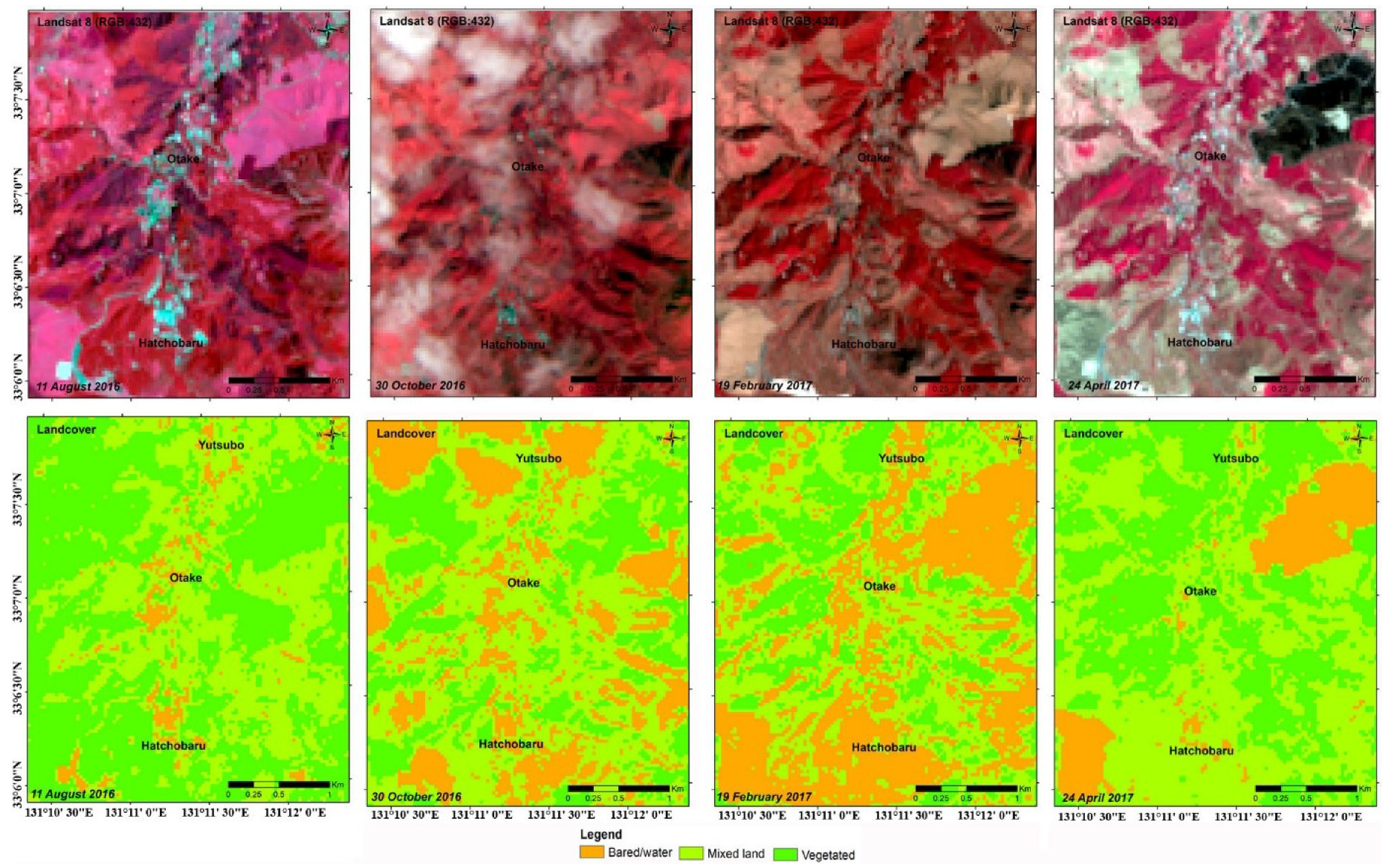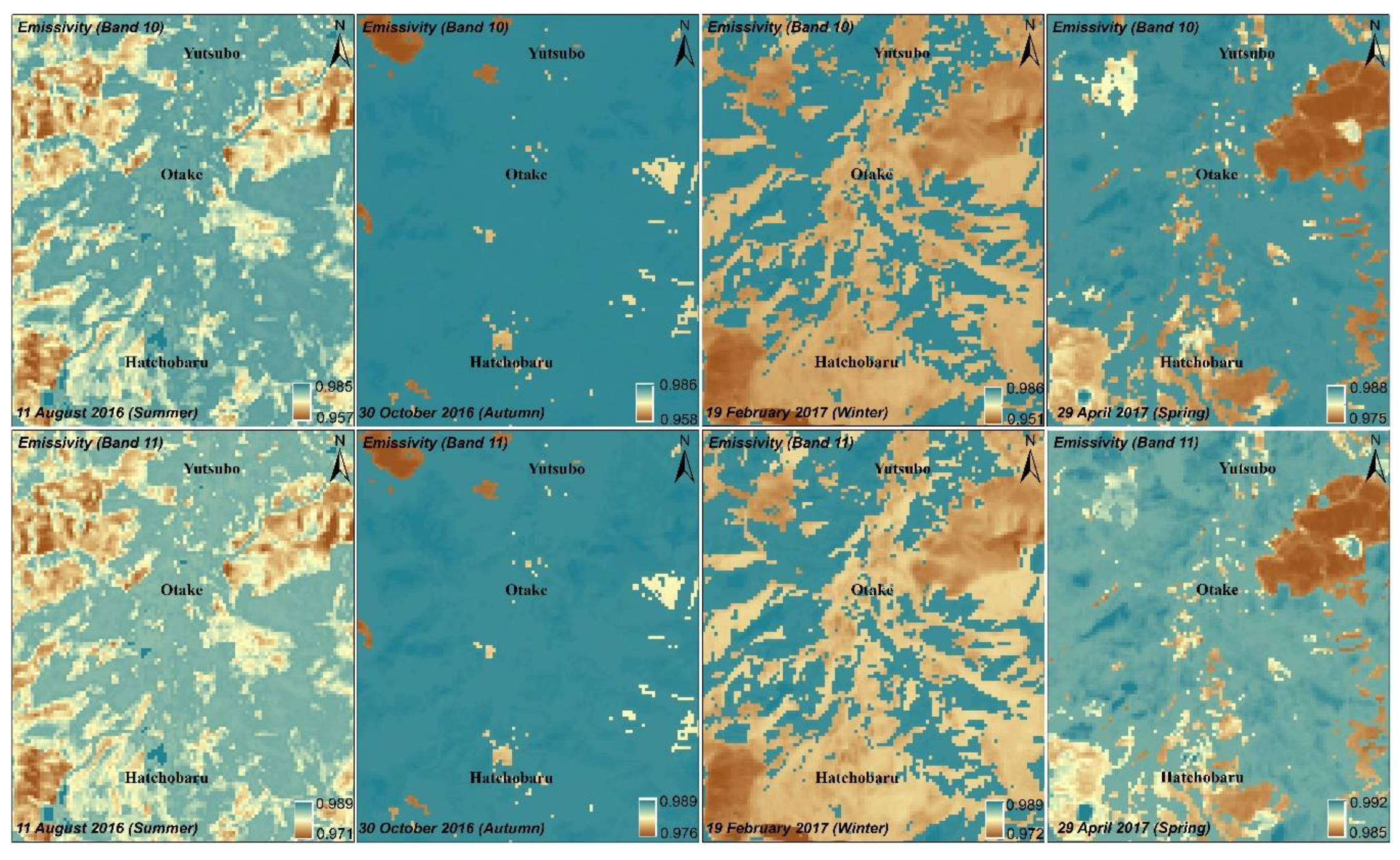This SW method reduces the requirements of the detail atmospheric data [37]. The SW method is used widely from a variety of thermal infrared sensors, such as ASTER, and Landsat, among others, because of its simplicity, efficiency, and insensitivity to atmospheric uncertainty. The only prior requirement of the SW algorithm is the emissivity of the land cover of the study area. For this reason, the SW algorithm was used in the current study to calculate the LST from the ASTER thermal infrared data. There are various approaches to predicting land surface emissivity from normalized differential vegetation index (NDVI) values [28,29]. The NDVI based emissivity method is very popular and is used to retrieve emissivity at a 15 m resolution for soil, vegetation, and water bodies efficiently, contrasting the TES method used to retrieve the emissivity of a 90 m resolution. In the case of the Landsat 8 images, it is well known and documented that the TIRS has suffered from a stray light problem since the launch of this satellite [39]. Although an algorithm was applied to correct the stray light problem, and the corrected TIRS data was supplied from February 2017, it was still not recommended to apply the TIRS band 11 for the split-window algorithm [39].

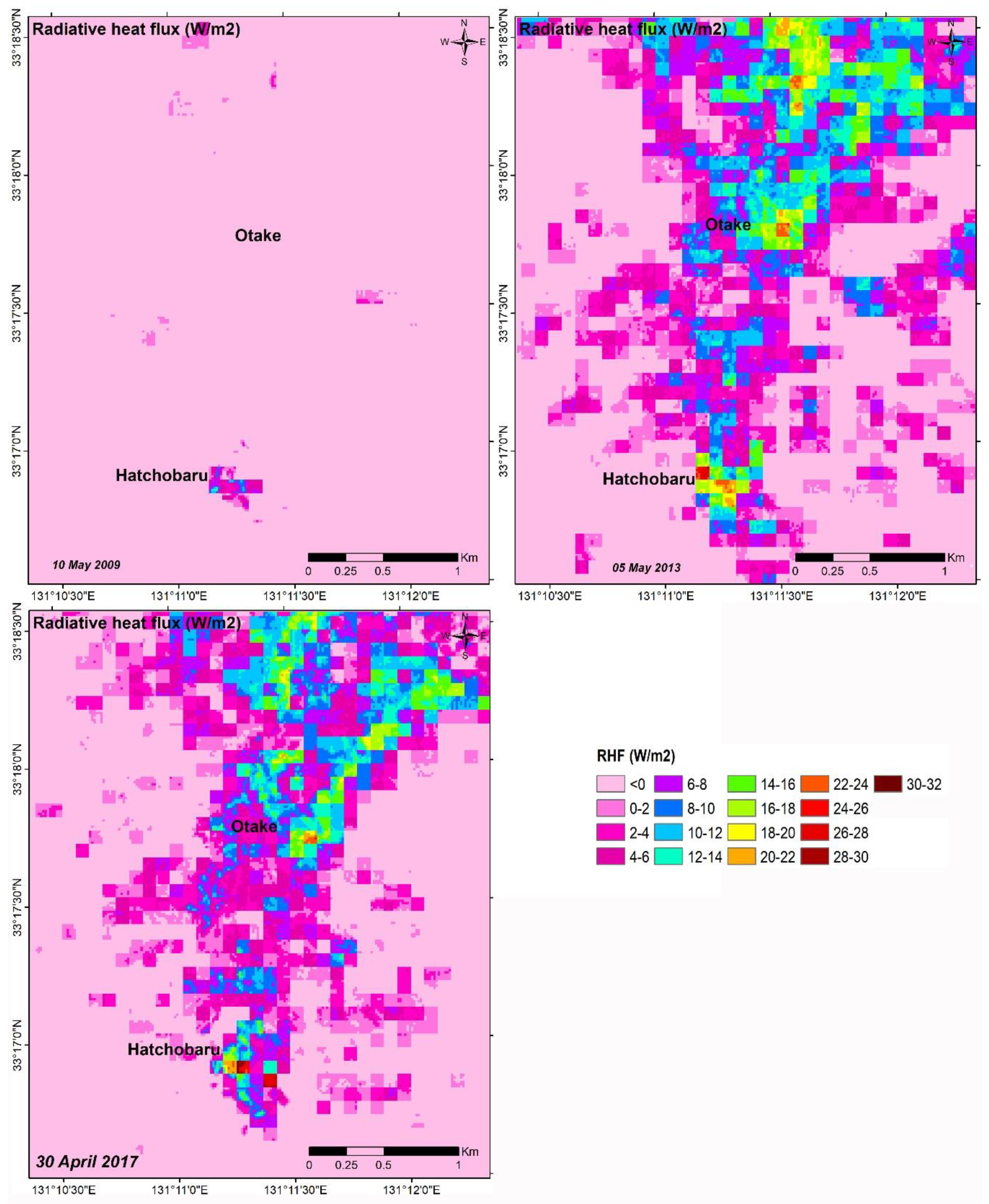
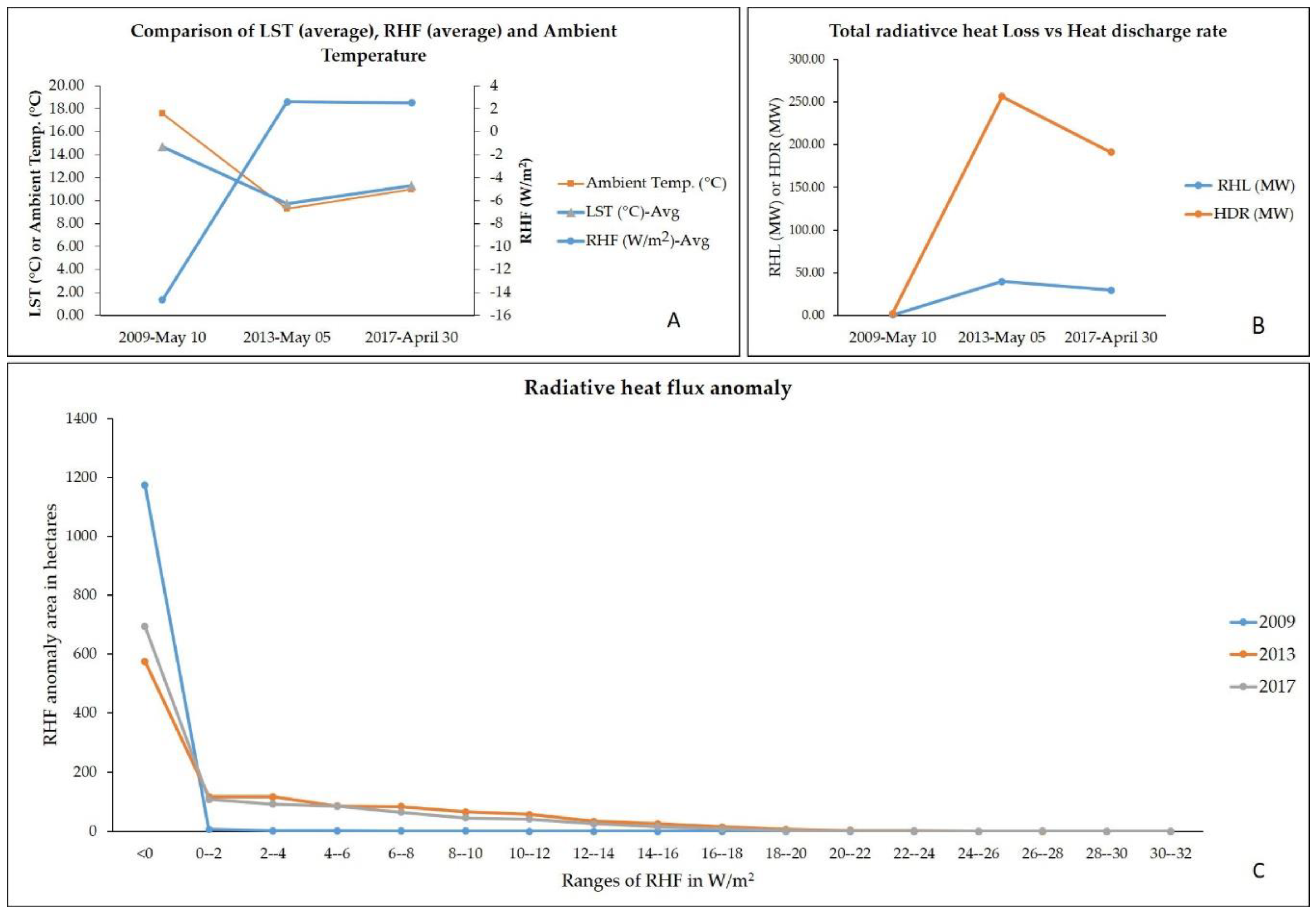
The heat losses monitored using the ASTER TIR data from 2009 to 2017 show that the highest total heat losses occurred in 2013 and lowest ones occurred in 2009, although the highest pixel value of the RHF was recorded in 2017, and the lowest one in 2009. Based on previous studies regarding the relationship between the RHF and HDR (15% ± 10%), we proposed HDR for the study area, after multiplying the total RHL by the coefficient of the relationship (15% or 6.49) [15,22]. 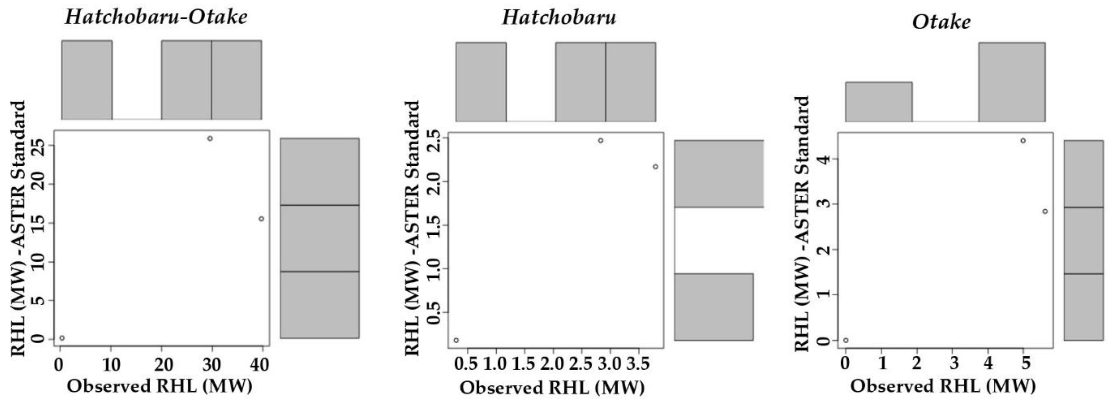The total heat losses or HDRs could be about 2.3 (±10%) MW, 257 (±10%) MW, and 191 (±10%) MW for 2009, 2013, and 2017, respectively, from our study area (Table 4 and Figure 7B). We compared the observed LST and RHF with the ASTER standard products based LST and RHF. The maximum LST and RHF was found to have a similar trend, but was lesser in value compared with the standard products observed, because of the resolution of the pixel (i.e., observed LST and RHF thematic map resolution of 15 m and the standard products resolution of 90 m). There is an inverse relationship between the pixel size and the retrieved maximum LST with a heterogeneous surface, which resulted in an inverse temperature radiance [40]. Hence, in the case of total RHL, we obtained a higher heat loss in 2017 than 2013 with ASTER standard products, opposite to that of the observed heat loss. This may be due to the emissivity value variations (high range for standards than observed) and resolutions (90 m for standard and 15 m for observed).

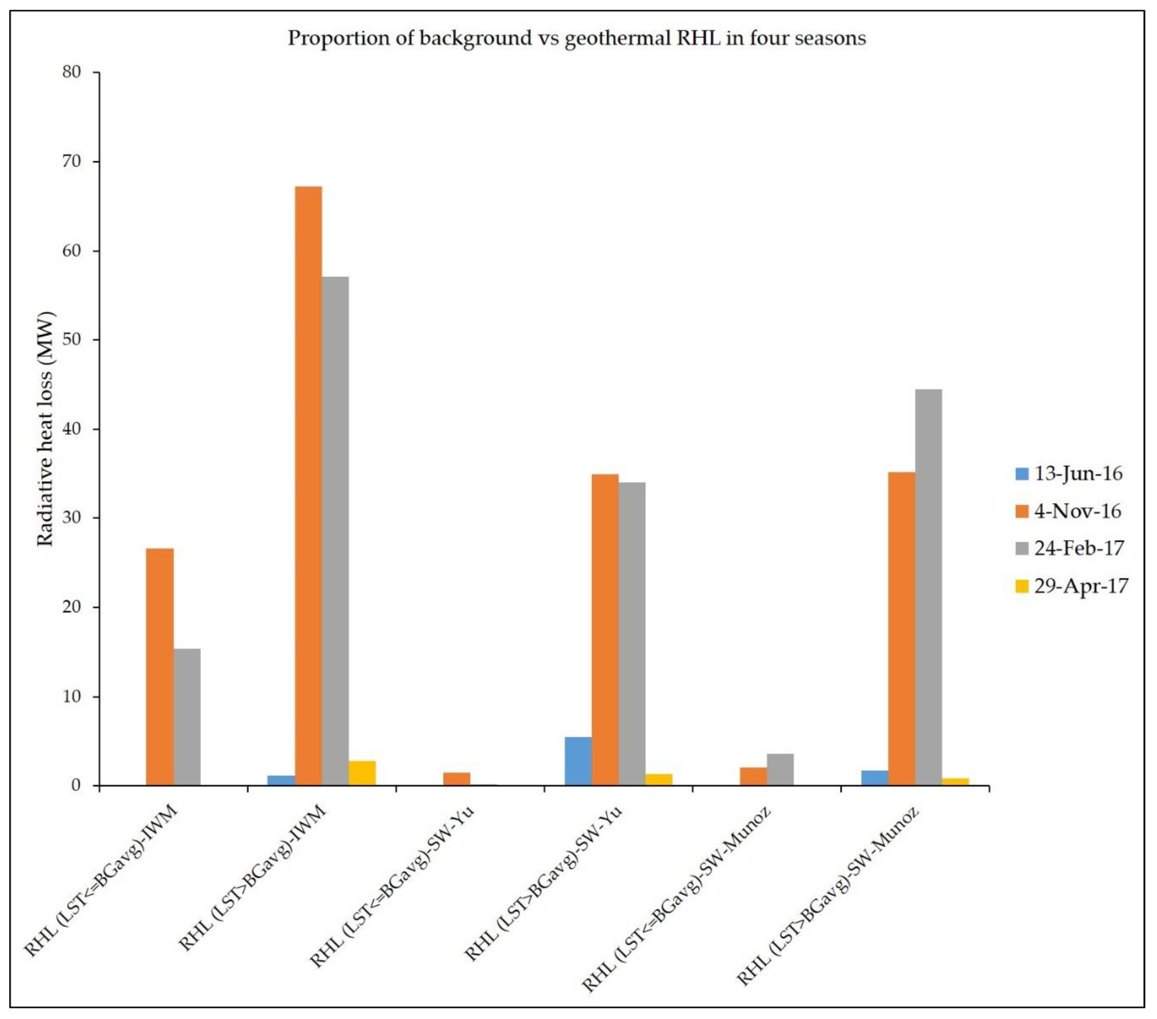
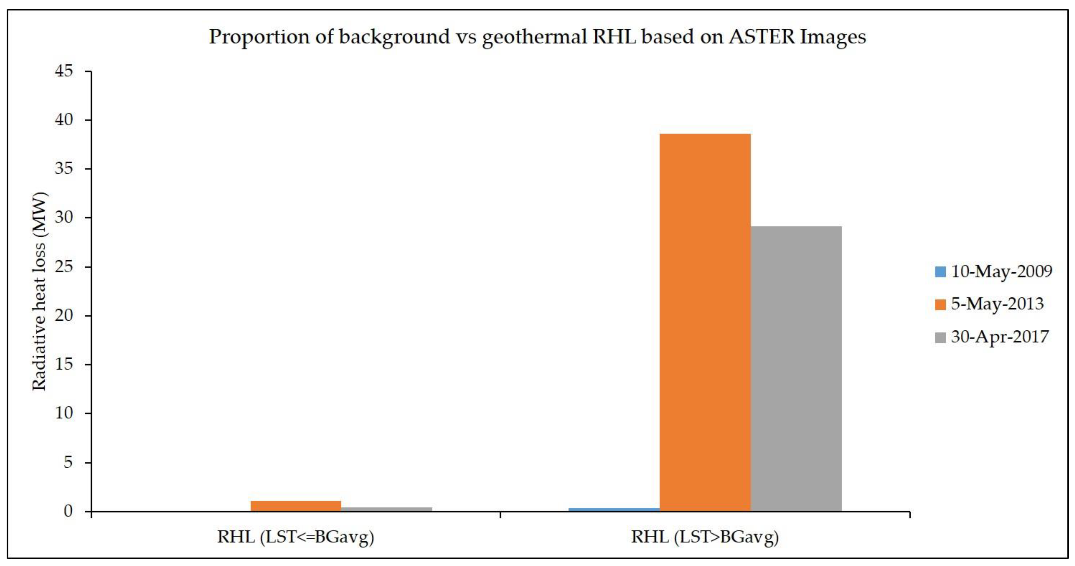
There is another source of uncertainty with the absorbed atmospheric temperature of land cover within the thermal ground in the case of the heat loss estimation, even with the nighttime thermal infrared data [40]. The background heat loss could be subtracted from the estimated heat loss of the study area, in order to derive the actual geothermal heat loss, but there were uncertainties or difficulties in selecting a similar topographic, altitude, land cover, and non-volcanic area as the background in and around the study area [40]. Moreover, our approach to evaluate the relative proportion of the RHL by pixels of background LST (average) on total RHL, may overestimate the geothermal RHL from total retrieved RHL. Based on the background LSTs (average), the contribution of the background was not so high on total the RHL, as the average background LSTs were less than expected (Figure 8 and Figure 21). Actually, if the background LST of any pixel is less than or equal to ambient, then the RHF value will be negative or zero, according to the Stefan–Boltzmann equation of RHF used in this study. As we added only the positive RHF, most of the background RHFs (mostly negative or zero) were not counted on the total RHL. Of course, some of the background pixels close to the geothermal area showed a higher LST than ambient, and resulted in RHL values more than the expected from the HO geothermal region. It seems that geothermal RHL still has some influence on the background, as we used the background average LST, which is much less than what is was originally in some of the pixels close to the HO geothermal area.

The variation of the thermal activity may be related to some of the reasons in this study area from 2009 to 2017, such as (1) the natural perturbation of geothermal system, (2) the impossibility of removing all of the background heat flux, and (3) the variation of heated water withdrawn from subsurface of the two geothermal power plants (i.e., Hatchobaru and Otake). It may possible to validate these results using the power plants information, such as the reservoir heated water temperature at well head, the water withdrawn volume, and the rate of electricity production during the period of the study, however, these data are not available to be used publicly from the authority of the power plants operating company.

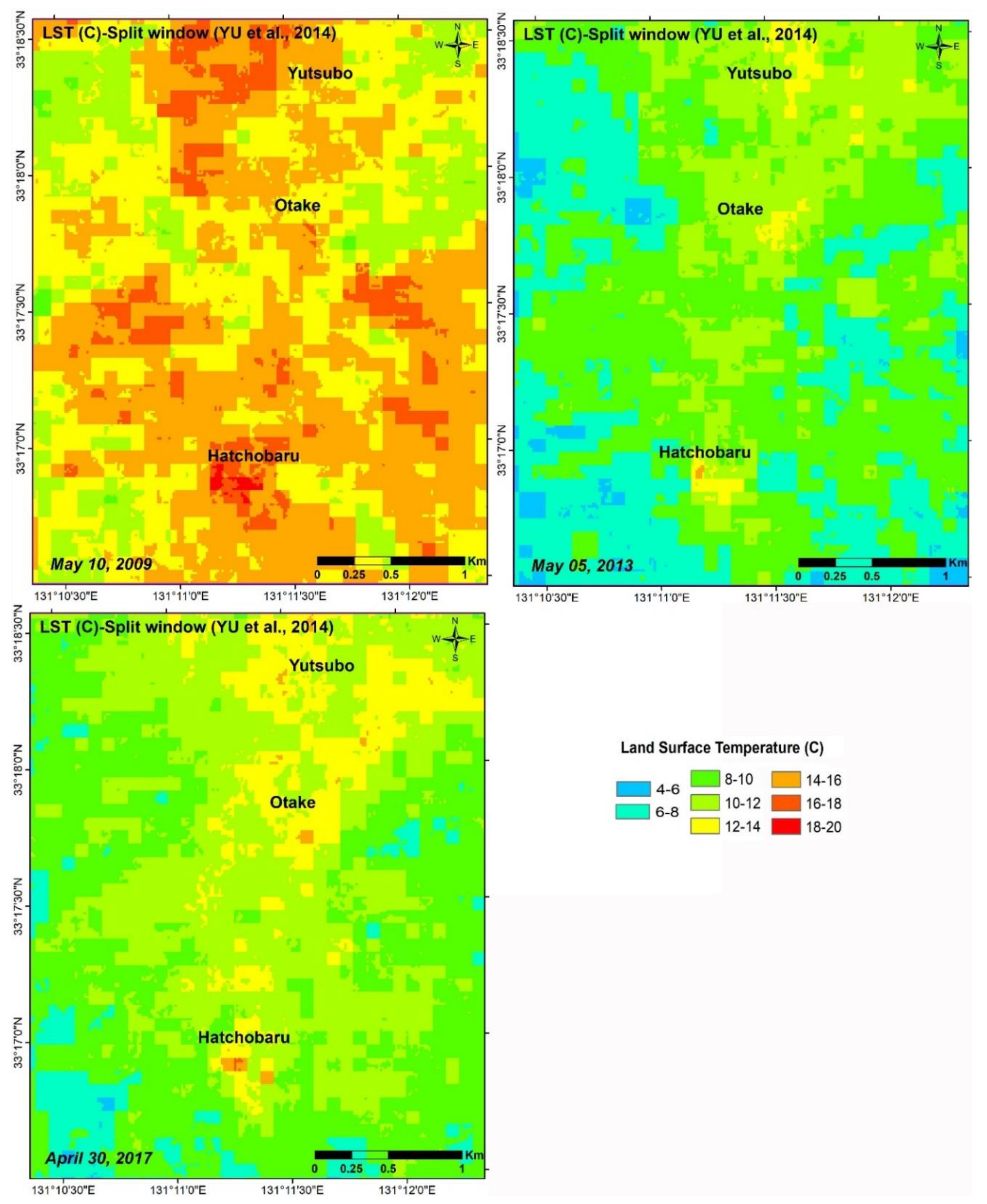
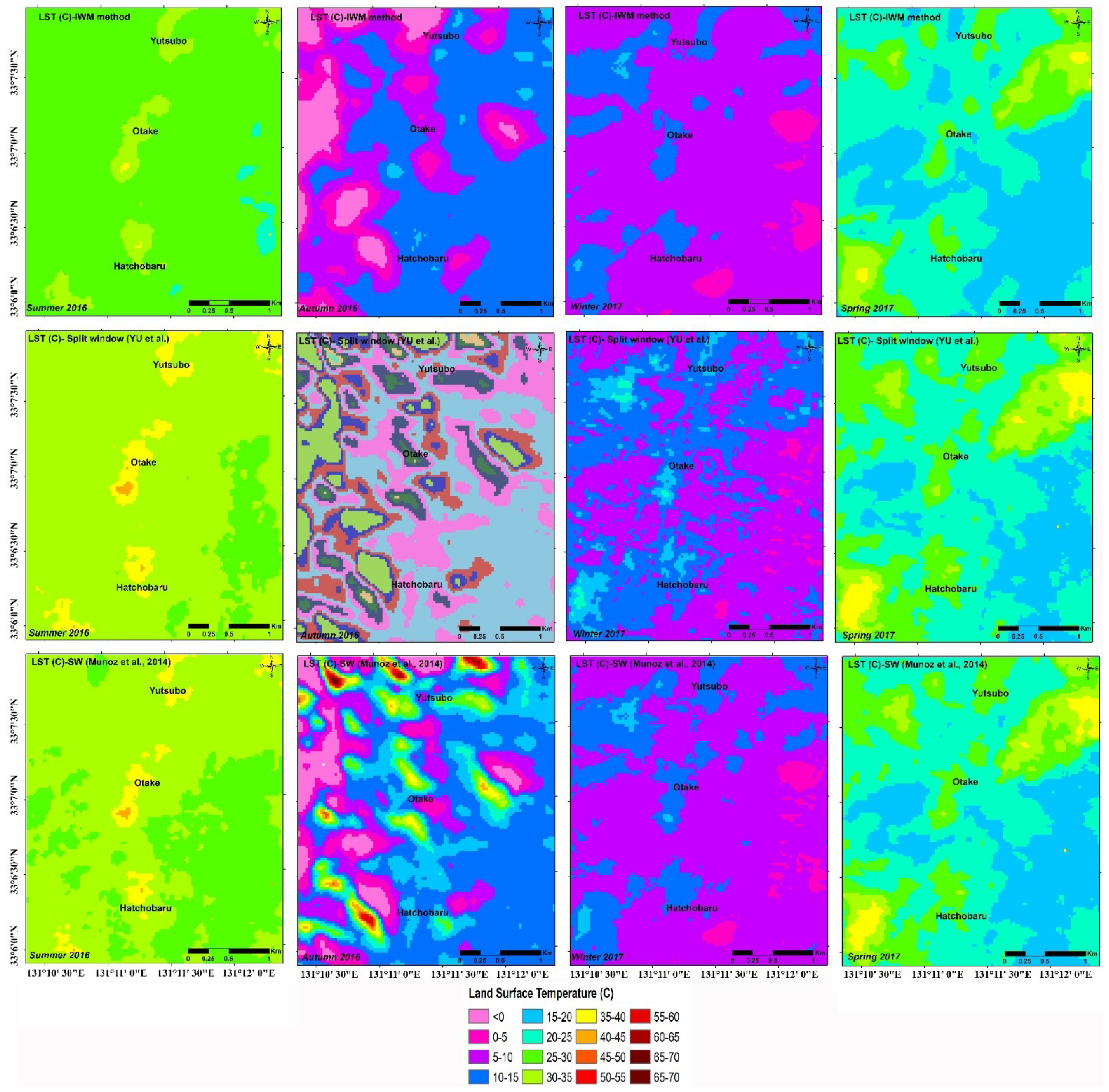
The day- and night-time LST results showed that much higher thermal anomalies or LSTs were established in the daytime than during the nighttime, reflecting the effect of solar insolation during the image acquisition. The autumn LST maps had high thermal anomalies related to cloud cover during the daytime. 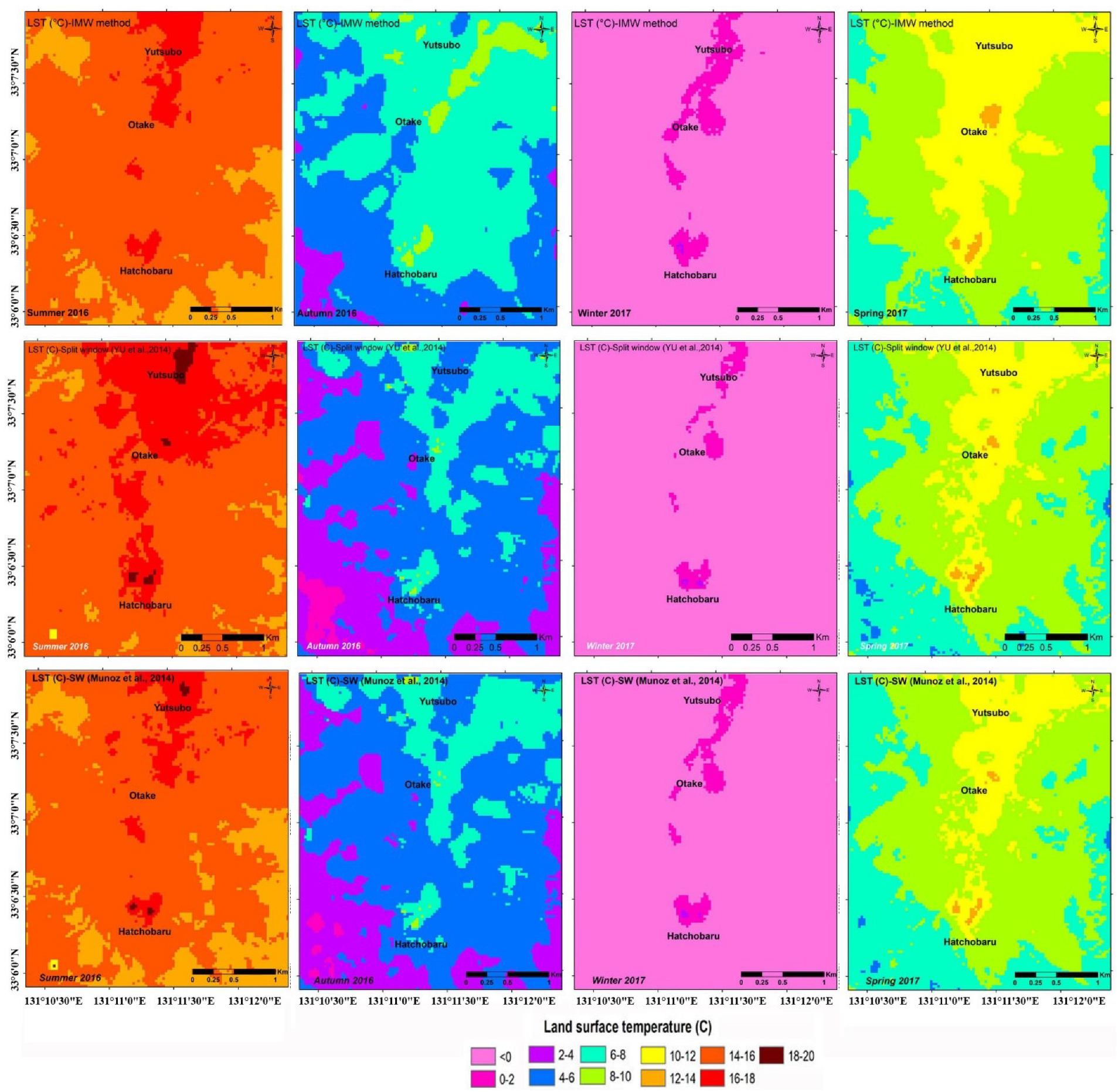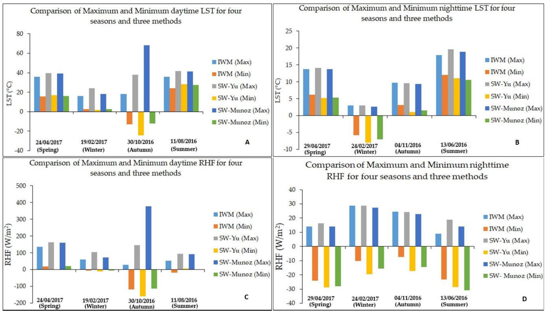This result coincided with a recent study of cloud effects on air temperature using MODIS TIR data, that is, clouds mainly influence the LST (max) estimation on the daytime image by affecting the relationship between the LST (max) and daytime LST, and hence, the error result of the LST (max) is larger in the daytime than in the nighttime [41]. The nighttime image analysis showed that higher thermal anomalies were associated with the HO geothermal system, with maximum LSTs recorded in the summer and the lowest ones recorded in the winter for all three conventional methods of the LST estimation using Landsat 8 TIRS data (Figure 13). The daytime maximum LSTs were about three, six to eight, two to seven, and two times that of the nighttime maximum LST, for the spring, winter, autumn, and summer seasons, respectively, with all three of the LST methods. 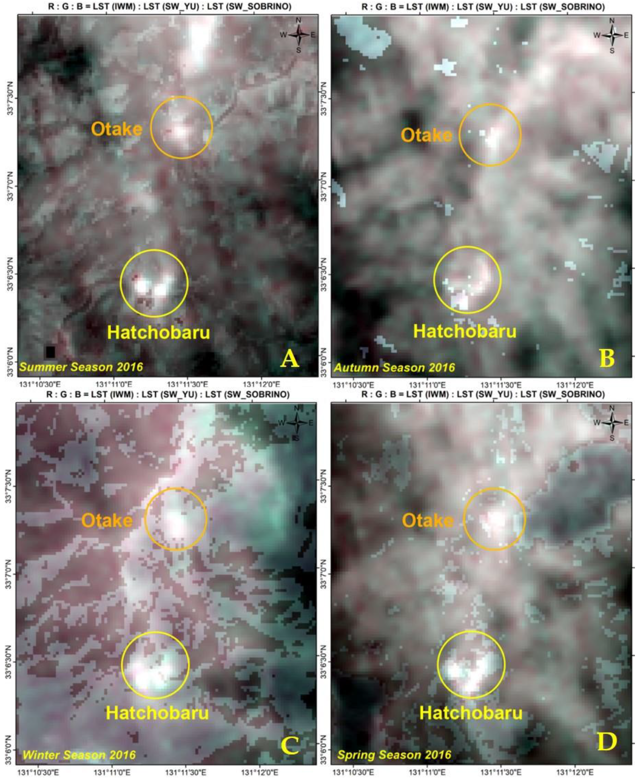All of the three methods showed a similar range of variations for the maximum LST during the day- and night-time in all of the seasons, except autumn (Table 5). The RGB combinations of LST values for all three of the methods showed high anomalies associated with the Hatchobaru, Otake, and Yutsubo hot spring areas. Although white pixels indicate the same LST for all three of the LST methods, different shades of color (R/G/B) indicate where one LST method is over- or under-estimated by the other LST methods, which might be due to the sensitivity of LST measurement of these methods (Figure 13). The IWM method shows a possible average error of about −0.05 K and a root mean square error (RMSE) of about 0.84 K, which is less than the single channel method (average error −2.86 K and RMSE 1.05 K) [21]. The possible source of the error in the case of a single channel or IWM method is the water vapor content in the atmospheric profile [21]. On the other hand, the RMSE of SW-Yu et al. is about 1.025 K, as the LST retrieval from band 11 has more uncertainty than band 10 [19]. In the case of SW, Jiménez-Muñoz et al., the average error is about 1.5–2.1 K, while the RMSE is below 1.5 K [20].

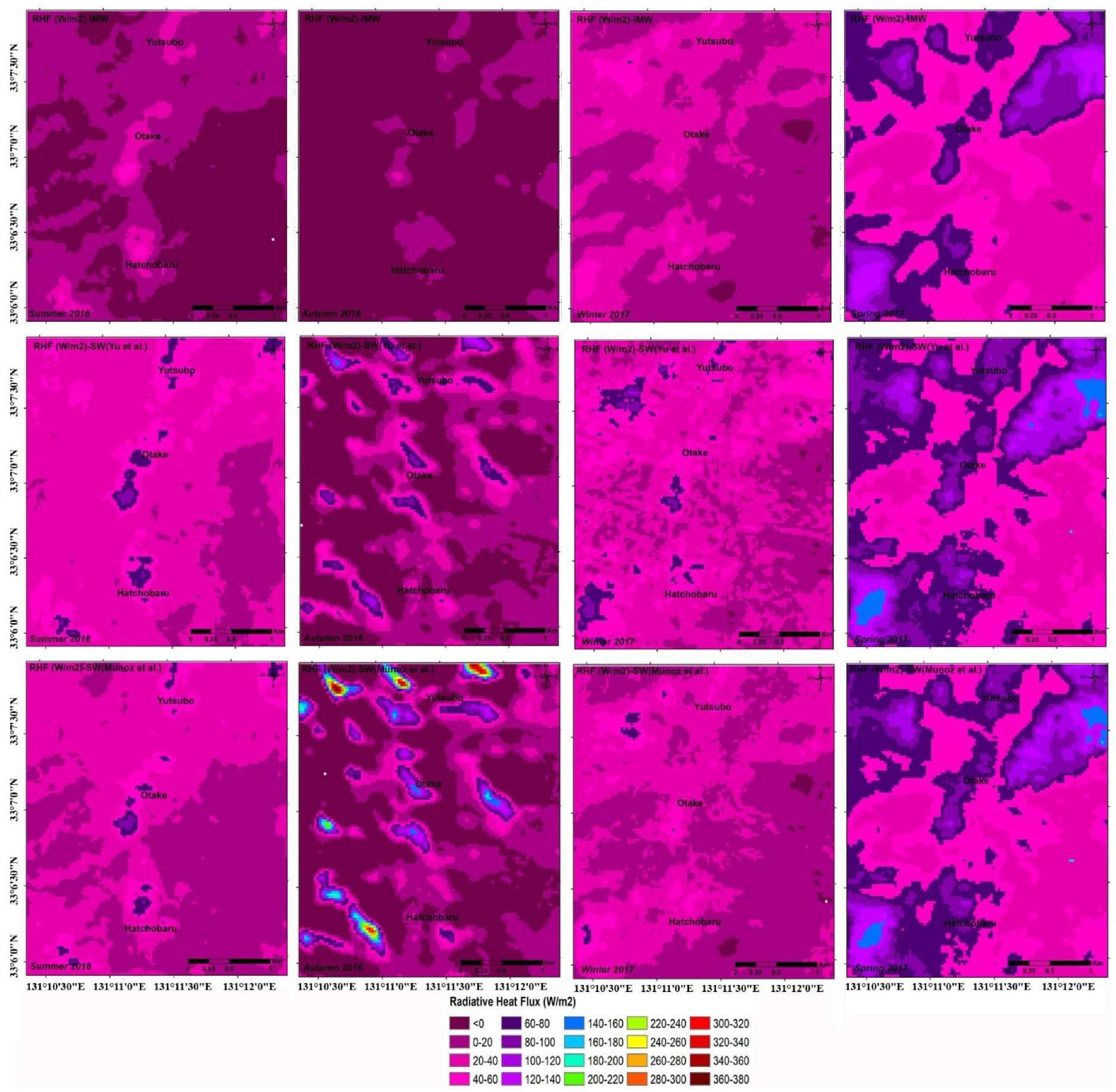
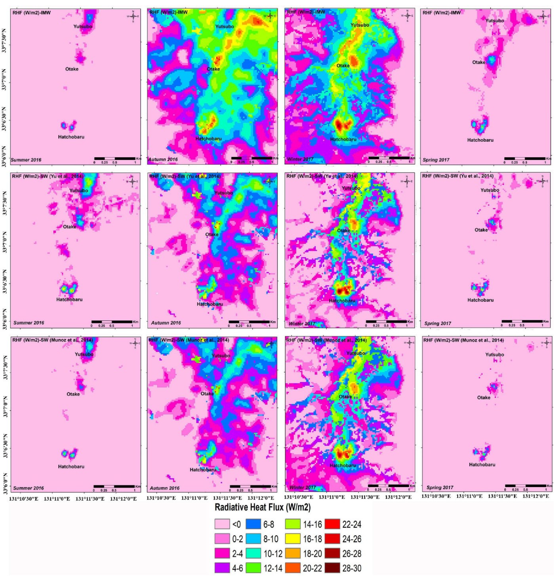
The daytime RHFs had high values in all seasons around the Hatchobaru and Otake hot spring areas, except in autumn, when the highest RHF values were related to cloud cover, especially in the LSTs derived from the SW algorithms. The nighttime radiative heat loss anomalies were linked to the OH geothermal area in all of the seasons. The daytime RHFs were much higher in all of the seasons because of the solar effects. The daytime maximum RHFs were about 10–11, 2–4, 1–17, and 5–7 times that of the nighttime maximum RHF, for the spring, winter, autumn, and summer seasons, respectively, with all three of the LST methods based the RHF. 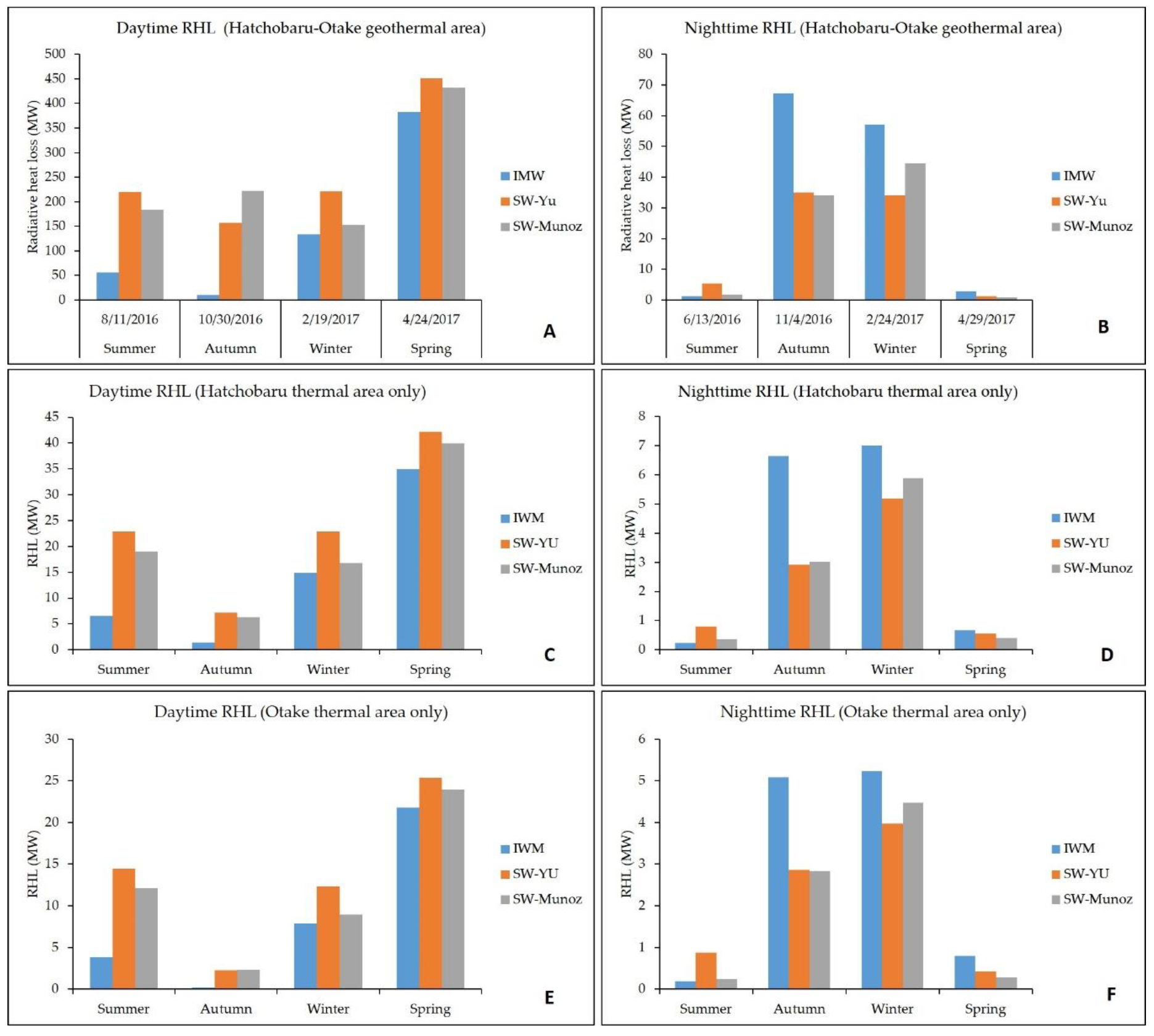These three methods showed a close range of variations of the maximum RHF during day- and night-time in all seasons, except autumn (Table 5). A comparison of all three of the LST estimation methods showed that the IMW algorithm derived maximum LSTs in all seasons, except summer. This may be due to the differences in the day- and night-time acquisition time, which are higher in summer (about two months) than in the other seasons (less than a month), resulting in the variation in emissivity. The result of IMW is quite different than the SW algorithm, as the SW method used band 10 as well as band 11, which is not recommended for LST, because of the light stray problem of the TIRS sensor of Landsat 8. Similar intra-seasonal trends were observed for all of the methods based on the 101-random point sampling of the nighttime LSTs of the study area. After using both the day- and night-time LSTs for estimating the total RHLs, we observed that the total RHLs derived using the SW-based LSTs were higher than those for the IMW-based LSTs in all seasons, except for summer (in daytime images). In the nighttime images, the IMW-based LSTs yielded total RHLs that were higher in all seasons, except for summer. 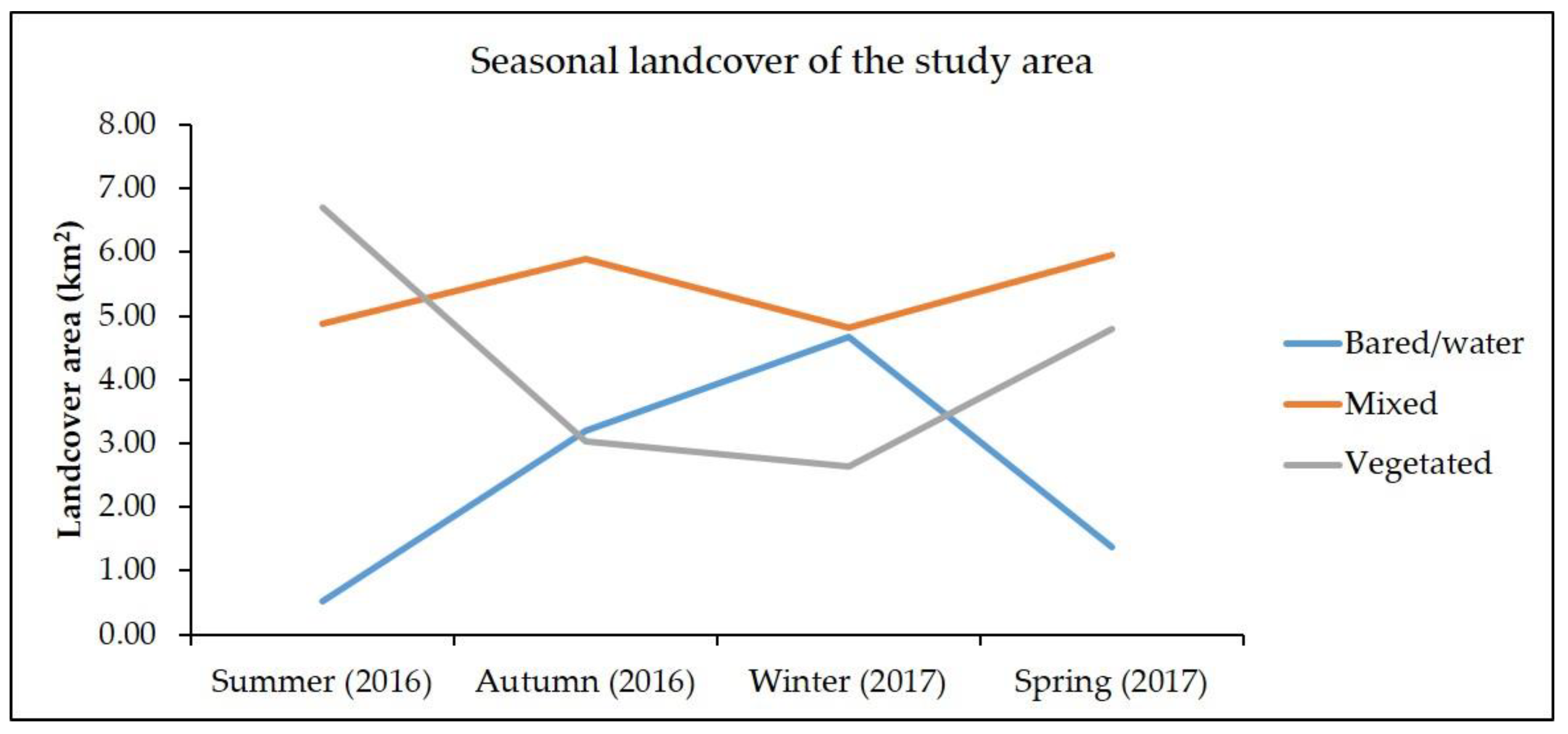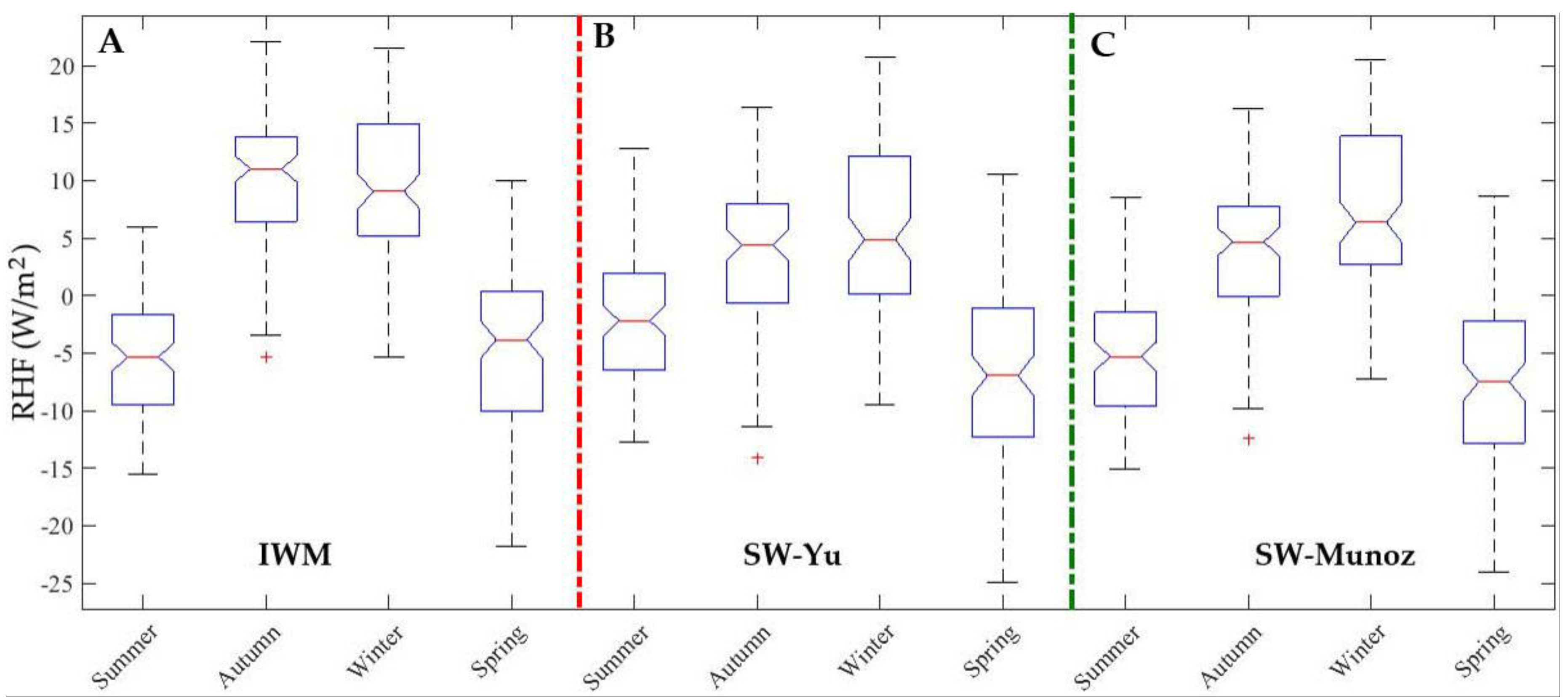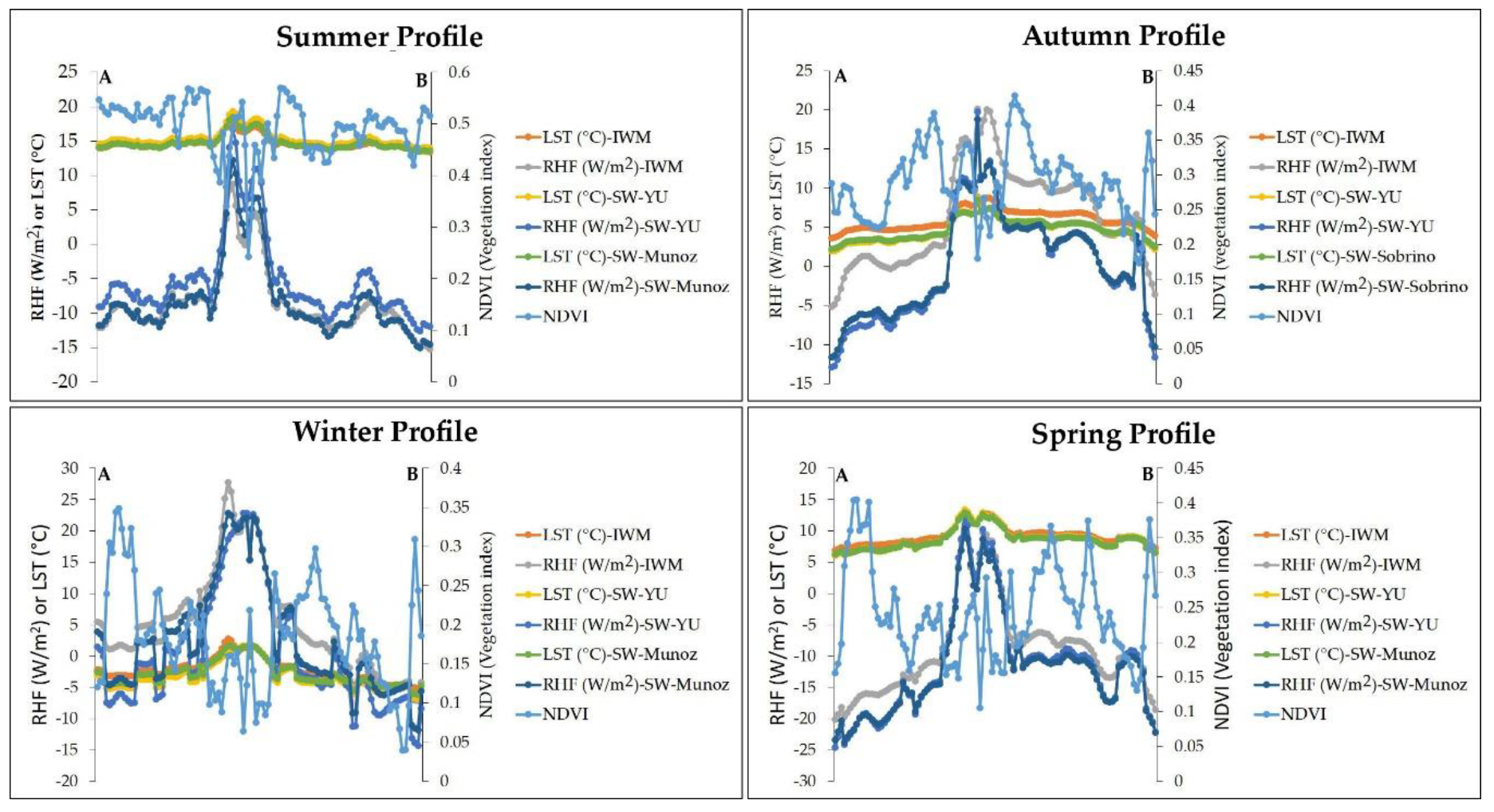The seasonal variations were significant in each season, with little variations in the applied three LST methods (Figure 18). Winter and autumn had higher RHFs, while summer and spring had lower RHFs in the nighttime TIR data, related to lower ambient temperatures. The RHFs were more or less similar in all three of the methods for the seasons of spring and summer. Exploring the relationships between RHF and LST against NDVI (or landcover) showed that the NDVI values of less than 0.5 (mixed or bare ground) were associated with higher LST and RHF values within the HO geothermal area.

The average heat flux of the continental crust is about 0.065 W/m² [40]. The heat flux is reported as about 21 W/m² (average) and about 37 W/m² (maximum) from an active thermal area of the Yellowstone national park, which is more than 300 times that of the continental heat flux [40]. In this study, we obtained a maximum heat flux of about 31 W/m², using nighttime ASTER TIR data, and about 29 W/m², using Landsat 8 TIRS data from the active HO geothermal area (Table 4 and Table 6).

We would like to suggest the IWM method for estimating LST using Landsat 8 TIRS data, considering the error of thermal band 11 as a result of the stray light problem of Landsat 8 TIRS sensor, the LST estimations accuracy (based on the source articles [19,20]), and the consistency of the LST results in three out of four seasons in this study. A significant limitation of this research is the lack of ground validation information due to the inaccessible fumaroles, and unavailable data of previous heat loss and power plants. However, we validated our retrieved RHL with ASTER standard products (AST_05, emissivity and AST_08, temperature), based on the results of total RHL in this study, with strong Pearson correlation coefficients. As a first study for thermal status monitoring with comparison of method, and solar and seasonal effects, continuous nighttime satellite thermal infrared data of same month or seasons could be worth it for the long-term monitoring of thermal activity at the HO geothermal area, so as to help with the sustainability of the geothermal resource.

6. Conclusions

To address the issue of spatial heat loss from the HO geothermal area, we used ASTER and Landsat 8 images to monitor the geothermal heat loss from 2009 to 2017, compared with the solar effects, seasonal variation, and LST measurement methods in this study. Our study of the nighttime ASTER TIR data indicates that the thermal activity has undergone both an increase and decrease within the HO geothermal area from 2009 to 2017, keeping an uncertainty of the limited numbers of data. The RHLs were more in the Otake than Hatchobaru thermal area in the year of 2013 (~31%) and 2017 (~78%). The daytime heat losses were much higher than nighttime ones, because of solar effects on daytime Landsat 8 satellite images. The heat losses in all four seasons were distinct in both the daytime and nighttime Landsat images. The highest heat losses were in winter and autumn, while the lowest losses were in spring and summer in the nighttime satellite images. The heat losses calculated using the IMW-based LSTs were slightly higher than those of the SW algorithms. The HO geothermal area had higher LSTs as well RHLs in all of the seasons, compared with its surrounding non-thermal areas. The total RHLs ranged from 10 to 451 MW (after removing RHL by pixels with background LST-average on total RHL) in the daytime over all four seasons, with the highest values in spring and the lowest ones in autumn. In contrast, at night, the RHLs ranged from 1 to 67 MW (after removing RHL by pixels with background LST-average on total RHL), with the highest values in autumn and the lowest ones in spring, based on the Landsat 8 TIRS images. Individually, during the day, the RHLs ranged from 1–42 MW and 0.19–25 MW over all four seasons, from the Hatchobaru and Otake thermal area, respectively, with the highest values in spring and the lowest in autumn. At night, the RHLs ranged from 0.23–7 MW and 0.19–5 MW over all four seasons, from the Hatchobaru and Otake thermal area, respectively, with the highest in winter and the lowest in summer. In this study, we applied limited numbers of ASTER TIR data to monitor the geothermal activity of the study area from 2009 to 2017, because of the unavailability of the data, while the Landsat 8 OLI/TIRS seasonal data were used to evaluate the solar, seasonal, and methodological effects on the LST and RHF estimations.

References

1. Nishijima, J.; Fujimitsu, Y.; Ehara, S.; Kouno, E.; Yamauchi, M. Micro-gravity monitoring and repeated GPS survey at Hatchobaru geothermal field, central Kyushu, Japan. In Proceedings of the World Geothermal Congress, Antalya, Turkey, 24–29 April 2005. [Google Scholar]
2. Sasada, M. Development of Permeable Fractures in Geothermal Systems in the Japanese Islands—Two Contrasting Types of Geothermal Reservoir. World Geotherm. Congr. 1995, 1315–1318. [Google Scholar]
3. Fujino, T.; Yamasaki, T. Geologic and geothermal structure of the Hatchobaru field, central Kyushu, Japan. Geotherm. Resour. Counc. Trans. 1984, 8, 425–430. [Google Scholar]
4. Fukuda, M.; Ushijma, K.; Aosaki, K.; Yamamuro, N. Some Geothermal Measurements at the Otake Geothermal Area. Geothermics 1970, 2, 148–157. [Google Scholar] [CrossRef]
5. Yamasaki, T.; Matsumoto, Y.; Hayashi, M. The geology and hydrothermal alteration of the Otake geothermal area, Kujyo volcano group, Kyushu, Japan. Geothermics 1970, 2, 197–207. [Google Scholar] [CrossRef]
6. Hirowatari, K. Development—Related changes in the Hatchobaru geothermal system, Japan. Geochem. J. 1991, 25, 283–299. [Google Scholar] [CrossRef]
7. Ishitsuka, K.; Tsuji, T.; Matsuoka, T.; Nishijima, J.; Fujimitsu, Y. Heterogeneous surface displacement pattern at the Hatchobarugeothermal field inferred from SAR interferometry time-series. Int. J. Appl. Earth Obs. Geoinf. 2016, 44, 95–103. [Google Scholar] [CrossRef]
8. Ishii, K.; Ejima, Y.; Shimoike, T. Present status of the Otake and Hatchobaru geothermal power plants(ii)—on the exploration and research. N. Z. Geotherm. Workshop 1988, 10, 317–320. [Google Scholar]
9. Mia, M.B.; Fujimitsu, Y.; Nishijima, J. Thermal activity monitoring of an active volcano using Landsat 8/OLI-TIRS sensor images: A case study at the Aso volcanic area in southwest Japan. Geosciences 2017, 7, 118. [Google Scholar] [CrossRef]
10. Mia, M.B.; Nishijima, J.; Fujimitsu, Y. Exploration and monitoring geothermal activity using Landsat ETM+ images-A case study at Aso volcanic area in Japan. J. Volcanol. Geotherm. Res. 2014, 275, 14–21. [Google Scholar] [CrossRef]
11. Van der Meer, F.; Hecker, C.; Van Ruitenbeek, F.; Van der Werff, H.; De Wijkerslooth, C.; Wechsler, C. Geologic remote sensing for geothermal exploration: A review. Int. J. Appl. Earth Obs. Geoinf. 2014, 33, 255–269. [Google Scholar] [CrossRef]
12. Mia, M.B.; Bromley, C.J.; Fujimitsu, Y. Monitoring heat flux using Landsat TM/ETM+ thermal infrared data—A case study at Karapiti (‘Crater of the Moon’) thermal area, New Zealand. J. Volcanol. Geotherm. Res. 2012, 235, 1–10. [Google Scholar] [CrossRef]
13. Qin, Q.; Zhang, N.; Nan, P.; Chai, L. Geothermal area detection using Landsat ETM+ thermal infrared data and its mechanical analysis—A case study in Tengchong, China. Int. J. Appl. Earth Obs. Geoinf. 2011, 13, 552–559. [Google Scholar] [CrossRef]
14. Savage, S.L.; Lawrence, R.L.; Custer, S.G.; Jewett, J.T.; Powell, S.L.; Shaw, J.A. Review of Alternative Methods for Estimating Terrestrial Emittance and Geothermal Heat Flux for Yellowstone National Park Using Landsat Imagery. GISci. Remote Sens. 2010, 47, 460–479. [Google Scholar] [CrossRef]
15. Harris, A.J.L.; Lodato, L.; Dehn, J.; Spampinato, L. Thermal characterization of the Vulcano field. Bull. Volcanol. 2009, 71, 441–458. [Google Scholar] [CrossRef]
16. Newson, J.A.; O’Sullivan, M.J. Computer modelling of heat and mass flow in steaming ground at Karapiti Thermal Area, New Zealand. In Proceedings of the 29th Workshop on Geothermal Reservoir Engineering, Stanford, CA, USA, 26–28 January 2004. [Google Scholar]
17. Seward, A.; Ashraf, S.; Reeves, R.; Bromley, C. Improved environmental monitoring of surface geothermal features through comparisons of thermal infra-red, satellite remote sensing and terrestrial calorimetry. Geothermics 2018, 73, 60–73. [Google Scholar] [CrossRef]
18. Qin, Z.; Dall’, O.G.; Karnieli, A.; Berliner, P. Derivation of split window algorithm and its sensitivity analysis for retrieving land surface temperature from NOAA-AVHRR data. J. Geophys. Res. 2001, 106, 22655–22670. [Google Scholar] [CrossRef]
19. Yu, X.; Guo, X.; Wu, Z. Land Surface Temperature Retrieval from Landsat 8 TIRS—Comparison between Radiative Transfer Equation-Based Method, Split Window Algorithm and Single Channel Method. Remote Sens. 2014, 6, 9829–9852. [Google Scholar] [CrossRef] [Green Version]
20. Jiménez-Muñoz, J.C.; Sobrino, J.A.; Skokovic, D.; Mattar, C.; Cristobal, J. Land surface temperature retrieval methods from Landsat-8 thermal infrared sensor data. IEEE Geosci. Remote Sens. Lett. 2014, 11, 1840–1843. [Google Scholar] [CrossRef]
21. Wang, F.; Qin, Z.; Song, C.; Tu, L.; Karnieli, A.; Zhao, S. An Improved Mono-Window Algorithm for Land Surface Temperature Retrieval from Landsat 8 Thermal Infrared Sensor Data. Remote Sens. 2015, 7, 4268–4289. [Google Scholar] [CrossRef] [Green Version]
22. Mia, M.B.; Bromley, C.J.; Fujimitsu, Y. Monitoring heat losses using Landsat ETM + thermal infrared data: A case study in Unzen geothermal field, Kyushu, Japan. Pure Appl. Geophys. 2013, 170, 2263–2271. [Google Scholar] [CrossRef]
23. Yuhara, K.; Akibayashi, S. Flow of reinjected water and transmissibility distribution estimated by a tracer test in Otake geothermal reservoir, Japan. J. Volcanol. Geotherm. Res. 1983, 16, 205–219. [Google Scholar] [CrossRef]
24. Taguchi, S.; Nakamura, M. Subsurface thermal structure of the Hatchobaru geothermal system, Japan, determined by fluid inclusion study. Geochem. J. 1991, 25, 301–314. [Google Scholar] [CrossRef]
25. Talay, T.A. Introduction to the Aerodynamics of Flight; Scientific and Technical Information Office, National Aeronautics and Space Administration: Washington, DC, USA, 1975.
26. Airbus, A.G. Getting to grips with aircraft performance. Cust. Serv. Blagnac 2002, 2, 11–16. [Google Scholar]
27. Qin, Z.; Li, W.; Gao, M.; Zhang, H.O. An algorithm to retrieve land surface temperature from ASTER thermal band data for agricultural drought monitoring. In Proceedings of the Remote Sensing for Agriculture, Ecosystems, and Hydrology VIII, Stockholm, Sweden, 11–13 September 2006. [Google Scholar]
28. Valor, E.; Caselles, V. Mapping Land Surface Emissivity from NDVI: Application to European, African, and South American Areas. Remote Sens. Environ. 1996, 57, 167–184. [Google Scholar] [CrossRef]
29. Van de Griend, A.A.; Owe, M. On the Relationship between Thermal Emissivity and the Normalized Difference Vegetation Index for Natural Surfaces. Int. J. Remote Sens. 1993, 14, 1119–1131. [Google Scholar] [CrossRef]
30. Sobrino, J.A.; Jimenez-Munoz, J.C.; Soria, G.; Romaguera, M.; Guanter, L.; Moreno, J.; Plaza, A.; Martincz, P. Land Surface Emissivity Retrieval from Different VNIR and TIR Sensors. IEEE Trans. Geosci. Remote Sens. 2008, 46, 316–327. [Google Scholar] [CrossRef]
31. Bromley, C.J.; van Manen, S.M.; Mannington, W. Heat flux from steaming ground: Reducing uncertainties. In Proceedings of the 36th Workshop on Geothermal Reservoir Engineering, Stanford, CA, USA, 31 January–2 February 2011. [Google Scholar]
32. Qin, Z.; Karnieli, A.; Berliner, P. A mono-window algorithm for retrieving land surface temperature from Landsat TM data and its application to the Israel–Egypt border region. Int. J. Remote Sens. 2001, 22, 3719–3746. [Google Scholar] [CrossRef]
33. Sobrino, J.A.; Li, Z.-L.; Stoll, M.P.; Becker, F. Multi-channel and multi-angle algorithms for estimating sea and land surface temperature with ASTR data. Int. J. Remote Sens. 1996, 17, 2089–2114. [Google Scholar] [CrossRef]
34. Jiménez-Muñoz, J.C.; Sobrino, J.A. Split-Window Coefficients for Land Surface Temperature Retrieval from Low-Resolution Thermal Infrared Sensors. IEEE Geosci. Remote Sens. Lett. 2008, 5, 806–809. [Google Scholar] [CrossRef]
35. Wessa, P.; Office for Research Development and Education. Pearson Correlation (v1.0.13) in Free Statistics Software (v1.2.1). 2017. Available online: https://www.wessa.net/rwasp_correlation.wasp (accessed on 19 August 2018).
36. Li, Z.-L.; Tang, B.-H.; Wu, H.; Ren, H.; Yan, G.; Wan, Z.; Trigo, I.F.; Sobrino, J.A. Satellite-derived land surface temperature: Current status and perspectives. Remote Sens. Environ. 2013, 131, 14–37. [Google Scholar] [CrossRef] [Green Version]
37. Ren, H.; Ye, X.; Liu, R.; Dong, J.; Qin, Q. Improving Land Surface Temperature and Emissivity Retrieval from the Chinese Gaofen-5 Satellite Using a Hybrid Algorithm. IEEE Trans. Geosci. Remote Sens. 2018, 56, 1080–1090. [Google Scholar] [CrossRef]
38. Gillespie, A.; Rokugawa, S.; Matsunaga, T.; Cothern, J.S.; Hook, S.; Kahle, A.B. A temperature and emissivity separation algorithm for Advanced Spaceborne Thermal Emission and Reflection Radiometer (ASTER) images. IEEE Trans. Geosci. Remote Sens. 1998, 36, 1113–1126. [Google Scholar] [CrossRef]
39. Gerace, A.; Montanaro, M. Derivation and validation of the stray light correction algorithm for the thermal infrared sensor onboard Landsat 8. Remote Sens. Environ. 2017, 191, 246–257. [Google Scholar] [CrossRef]
40. Vaughan, R.G.; Keszthelyi, L.P.; Lowenstern, J.B.; Jaworowski, C.; Heasler, H. Use of ASTER and MODIS thermal infrared data to quantify heat flow and hydrothermal change at Yellowstone National Park. J. Volcanol. Geotherm. Res. 2012, 233–234, 72–89. [Google Scholar] [CrossRef]
41. Zhang, H.; Zhang, F.; Zhang, G.; He, X.; Tian, L. Evaluation of cloud effects on air temperature estimation using MODIS LST based on ground measurements over the Tibetan Plateau. Atmos. Chem. Phys. 2016, 16, 13681–13696. [Google Scholar] [CrossRef] [Green Version]
Figure 1. Location of the Hatchobaru–Otake (HO) geothermal area. Background (hillshade) and contours (elevation in meters above mean sea level), prepared using Shuttle Radar Topography Mission digital elevation model values. Our study area was about 12 km2. The profile ‘A–B’ was used to compare the land surface temperature, radiative heat flux, and normalized difference vegetation index values of the study area. Heat loss was also monitored separately for the Hatchobaru and Otake geothermal area, shown as circles. The Aso-san meteorological station (AMeDAS, Automated Meteorological Data Acquisition System) is located near the crater of the Aso volcano, about 27 km southwest of the study area (32°52.8′N and 131°04.4′E; altitude is about 1142.3 m above mean sea level), shown with a rectangle in the index map of Kyushu Island.
Remotesensing 10 01430 g001
Figure 2. Geologic map of the Otake–Hatchobaru geothermal area (modified after the literature [24]). Crosshatched area = early Pleistocene Hohi volcanic rocks; others = middle–late Pleistocene Kujyu volcanic rocks.
Remotesensing 10 01430 g002
Figure 3. Satellite image processing flow chart used in this study. Daytime and nighttime images from both satellite sensors were used to calculate the emissivity and land surface temperatures using the various methods listed above. NIR—near infrared; TIR—thermal infrared; NDVI—normalised difference vegetation index; RHF—radiative heat flux; HDR—heat discharge rate.
Remotesensing 10 01430 g003
Figure 4. False colour composites of red/green/blue (RGB) visible bands of ASTER satellite data for the study area for 2009, 2013, and 2017 (top row). The bottom row shows the maps of the landcover types within the study area for 2009, 2013, and 2017. Locations of the Hatchobaru, Otake, and Yutsubo hot spring areas are shown on all of the images.
Remotesensing 10 01430 g004
Figure 5. Land surface temperatures (LSTs) for the study area for 2009, 2013, and 2017, derived from nighttime ASTER thermal infrared data, using the split-window method from the literature [19].
Remotesensing 10 01430 g005
Figure 6. Radiative heat flux (W/m2) maps derived from the ASTER thermal infrared images of the Hatchobaru–Otake geothermal area for 2009, 2013, and 2017.
Remotesensing 10 01430 g006
Figure 7. Changes in land surface temperatures (LST), radiative heat flux (RHF), and ambient temperature from 2009 to 2017 (A); RHF anomaly areas for 2009, 2013, and 2017 (C); and changes in total radiative heat loss (RHL) and heat discharge rate (HDR) from 2009 to 2017 for the Hatchobaru–Otake geothermal area (B).
Remotesensing 10 01430 g007
Figure 8. Plot shows the RHL contributed by the pixels with LST < or = background vs. LST < background, of the study area from 2009 to 2017. RHL—radiative heat loss; LST—land surface temperature; BGavg—background LST (average); BGmin—background LST (min); BGmax—background LST (max).
Remotesensing 10 01430 g008
Figure 9. High level ASTER standard product of the surface kinetic temperature (AST_08) of the HO geothermal area for the year of 2009, 2013, and 2017 ((top) row). RHFs are shown in the (bottom) row, retrieved from the ASTER standard products of surface emissivity (AST_05) and surface kinetic temperature (AST_08) of the study area for the year of 2009, 2013 and 2017.
Remotesensing 10 01430 g009
Figure 10. Scatter plot and histogram between the observed and standard ASTER products base RHL from the study area.
Remotesensing 10 01430 g010
Figure 11. False colour composites of near infrared/red/green bands of the Landsat 8 OLI images as red/green/blue (RGB) of the study area for each season (top row). The bottom row shows the land cover types in each season.
Remotesensing 10 01430 g011
Figure 12. Emissivity values for the study area in each season. The emissivity values derived from Landsat 8 band 10 are shown in the (top) row, while the emissivity values derived from Landsat band 11 are shown in the (bottom) row. The season is shown along the bottom of each image.
Remotesensing 10 01430 g012
Figure 13. Comparison of the areas of various land cover types within the study area for four seasons covering the period from June 2016 to April 2017.
Remotesensing 10 01430 g013
Figure 14. Seasonal land surface temperatures (LSTs) derived from nighttime Landsat 8 images using three different methods are shown as RGB composites. Panels (AD) show the LSTs for summer through spring, based on the improved mono-window and split-window algorithms of Yu et al. [19] and Jiménez-Muñoz et al., respectively, [20] for estimating the LSTs as red, green, and blue colour components of the composite. The white pixels identify the highest anomalies in the LST values, based on all of the methods. The circles are the thermal anomaly areas of Hatchobaru and Otake, used for the RHL estimation separately.
Remotesensing 10 01430 g014
Figure 15. Seasonal land surface temperatures (LST) within the study area derived from daytime Landsat 8 thermal infrared data. The LSTs of each season processed using the improved mono-window (IMW) algorithm are shown in the (top) row; the LSTs of each season processed using the split window (SW) algorithm of Yu et al. [19] are shown in the (middle) row; while the LSTs for each season processed using the SW algorithm of Jiménez-Muñoz et al. [20] are shown in the (bottom) row. Seasons are arranged in the order of summer, autumn, winter, and spring, in all of the rows.
Remotesensing 10 01430 g015
Figure 16. Seasonal land surface temperatures (LSTs) for the study area derived from nighttime Landsat 8 thermal infrared data. The LSTs for each season processed using the improved mono-window (IMW) algorithm are shown in the (top) row; LSTs for each season processed using the split-window (SW) algorithm of Yu et al. [19] are shown in the (middle) row; while the LSTs for each season processed using the SW algorithm of Jiménez-Muñoz et al. [20] are shown in the (bottom) row. The seasons are arranged in the order of summer, autumn, winter, and spring, in all of the rows.
Remotesensing 10 01430 g016
Figure 17. Seasonal radiative heat flux (RHF) within the study area for the daytime Landsat 8 thermal infrared data. The RHFs for each season processed using the improved mono-window (IMW) algorithm are shown in the (top) row; the RHFs for each season processed using the split-window (SW) algorithm of Yu et al. [19] are shown in the (middle) row; while the RHFs for each season processed using the SW algorithm of Jiménez-Muñoz et al. [20] are shown in the (bottom) row. The seasons are arranged in the order of summer, autumn, winter, and spring, in all of the rows.
Remotesensing 10 01430 g017
Figure 18. Seasonal radiative heat flux (RHF) in the study area for nighttime Landsat 8 thermal infrared data. The RHFs for each season processed using the improved mono-window (IMW) algorithm are shown in the (top) row; the RHFs for each season processed using the split-window (SW) algorithm of Yu et al. [19] are shown in the (middle) row; while the RHFs for each season processed using the SW algorithm of Jiménez-Muñoz et al. [20] are shown in the (bottom) row. The seasons are arranged in the order of summer, autumn, winter, and spring, in all of the rows.
Remotesensing 10 01430 g018
Figure 19. Comparison of the highest and lowest land surface temperatures (LSTs) and the radiative heat fluxes (RHFs) obtained from the day- and night-time thermal infrared images of the study area in each season, using three distinct methods of LST estimation (AD). The daytime LST and RHF for the autumn season shows the unrealistic value for SW-Muñoz method due to some cloud coverage of this image. IMW—improved mono-window algorithm; SW-Yu—split-window algorithm of Yu et al. [19]; SW-Muñoz—split-window algorithm of Jiménez-Muñoz et al. [20].
Remotesensing 10 01430 g019
Figure 20. Total radiative heat loss from the study area for both the day- and night-time Landsat 8 images, calculated using all three methods of the LST estimation are shown as the Hatchobaru–Otake geothermal area as a whole (A,B), the Hatchobaru thermal area only (C,D), and the Otake thermal area (E,F). The Hatchobaru and Otake thermal area were selected based on the higher thermal anomaly, shown in Figure 13 as circles. IMW—improved mono-window algorithm; SW-Yu—split-window algorithm of Yu et al. [19]; SW-Muñoz—split-window algorithm of Jiménez-Muñoz et al. [20].
Remotesensing 10 01430 g020
Figure 21. Plot shows RHL contributed by pixels with LST < or = to the background (average) vs. LST < background (geothermal) of the study area from the four seasons. RHL—radiative heat loss; LST—land surface temperature; BGavg—background LST (average); IMW—improved mono-window algorithm; SW-Yu—split-window algorithm of Yu et al. [19]; SW-Muñoz—split-window algorithm of Jiménez-Muñoz et al. [20].
Remotesensing 10 01430 g021
Figure 22. Intra-seasonal variation in land surface temperatures (LSTs) estimated using all three methods for each season. The variation was calculated using 101 random point samples of the study area. IMW—improved mono-window algorithm; SW-Yu—split-window algorithm of Yu et al. [19]; SW-Muñoz—split-window algorithm of Jiménez-Muñoz et al. [20].
Remotesensing 10 01430 g022
Figure 23. Seasonal variation in radiative heat flux (RHF) calculated using 101 random point samples of RHF, derived using three methods of land surface temperature (LST) estimation, namely: (A) RHFs based on LSTs derived from the improved mono-window algorithm (IMW); (B) RHFs based on LSTs derived from the split-window algorithm of Yu et al. [19] (SW-Yu); and (C) RHFs based on LSTs derived from the split-window algorithm of Jiménez-Muñoz et al. [20] (SW-Muñoz).
Remotesensing 10 01430 g023
Figure 24. Variation in land surface temperature (LST) and radiative heat flux (RHF) as a function of the normalised difference vegetation index (NDVI) along profile A–B, shown in Figure 1. The LSTs and RHFs were calculated using all three of the following methods: IMW—improved mono-window algorithm; SW-Yu—split-window algorithm of Yu et al. [19]; and SW-Muñoz—split-window algorithm of Jiménez-Muñoz et al. [20]. The panels show the variation in each season.
Remotesensing 10 01430 g024