Measuring Landscape Albedo Using Unmanned Aerial Vehicles


1
Yale-NUIST Center on Atmospheric Environment & Jiangsu Key Laboratory of Agriculture Meteorology, Nanjing University of Information Science & Technology, Nanjing 210044, China
2
School of Forestry and Environmental Studies, Yale University, New Haven, CT 06511, USA
3
WeRobotics, 1812 Bolton Street, Baltimore, MD 21217, USA
4
Center for Earth Observation, Yale University, New Haven, CT 06511, USA
5
Key Laboratory of Transportation Meteorology, China Meteorological Administration & Jiangsu Institute of Meteorological Sciences, Nanjing 210009, China
*
Authors to whom correspondence should be addressed.
Remote Sens. 2018, 10(11), 1812; https://0-doi-org.brum.beds.ac.uk/10.3390/rs10111812
Submission received: 11 September 2018
/
Revised: 11 November 2018
/
Accepted: 13 November 2018
/
Published: 15 November 2018
(This article belongs to the Special Issue Remotely Sensed Albedo)
Abstract
:Surface albedo is a critical parameter in surface energy balance, and albedo change is an important driver of changes in local climate. In this study, we developed a workflow for landscape albedo estimation using images acquired with a consumer-grade camera on board unmanned aerial vehicles (UAVs). Flight experiments were conducted at two sites in Connecticut, USA and the UAV-derived albedo was compared with the albedo obtained from a Landsat image acquired at about the same time as the UAV experiments. We find that the UAV estimate of the visibleband albedo of an urban playground (0.037 ± 0.063, mean ± standard deviation of pixel values) under clear sky conditions agrees reasonably well with the estimates based on the Landsat image (0.047 ± 0.012). However, because the cameras could only measure reflectance in three visible bands (blue, green, and red), the agreement is poor for shortwave albedo. We suggest that the deployment of a camera that is capable of detecting reflectance at a near-infrared waveband should improve the accuracy of the shortwave albedo estimation.
1. Introduction
Surface albedo is a key parameter in the surface energy balance, and it therefore plays an important role in land–climate interactions. As a key biophysical property of land ecosystems, surface albedo can change throughout the season, due to changes in the vegetation morphology, and it can also be affected by sky conditions [1]. Quantification of the surface albedo at the landscape scale is still subject to many sources of uncertainty, especially over urban land [1,2].
Satellite remote sensing has been widely used for the determination of land surface albedo [3,4,5,6]. An advantage of satellite monitoring is that it provides global coverage. New satellites can provide albedo measurements at reasonably high frequencies (2–3 days in the best case for Sentinel 2) and spatial resolutions (pixel size 10 m in the case of Sentinel 2, and several cm in the case of DigitalGlobe) to provide useful information for studies on ecosystem (tens of meters) to landscape (several kilometers to tens of kilometers) scales. However, all satellite measurements are biased towards cloud-free sky conditions. In urban landscapes with heavy haze pollution, retrieval of the true surface albedo from satellite imageries must remove signal contamination caused by particle scattering. Lightweight unmanned aerial vehicles (UAVs) as an alternative for albedo monitoring may be able to overcome these limitations. UAVs can cover areas ranging from 0.01 km2 to 100 km2, depending on battery life and type of UAV [7]. They provide measurements at sub-decimeter spatial resolutions, and they can be used to obtain data under both clear sky and cloudy conditions [8,9]. UAV experiments can be conducted at almost any time, and at any locations [10,11,12]. Furthermore, the labor and financial expense of UAVs are much lower than those of aircraft [13]. Finally, UAVs can measure albedos at locations that are not accessible by ground-based instruments, such as steep rooftops in cities.
In a typical UAV experiment, consumer-grade digital cameras are utilized as multispectral sensors, similar to their counterparts on board satellites, to measure the spectral radiance reflected by ground targets, typically in the red, green, and blue wavebands and occasionally with modification to include a near-infrared (NIR) waveband. These at-camera radiance data are stored as digital numbers (DN), usually with an 8-bit resolution ranging from 0 to 255, to represent the brightness of the targeted object [14]. Vegetation indices derived from the spectral information [15] allow for the monitoring of vegetation growth status [16,17,18], and the estimation of crop biomass [19]. Because the UAV flies below cloud layers, cloud interference is no longer a problem. Also, because of the low flight altitude in typical UAV missions, the at-sensor radiance is a direct measure of the actual surface reflected radiance, but this is not true for satellite monitoring (Even with UAVs flying at higher flight altitudes, atmospheric interference is still much less severe than with satellite monitoring). Alternatively, a UAV can be deployed as a platform to carry pyranometers to measure albedo. For example, Levy et al. measured surface albedo over vegetation using a ground-based pyranometer paired with a pyranometer mounted on a quadcopter [20].
Although increasingly being used to produce image mosaics and to construct 3D point clouds of surface features, consumer-grade cameras on board of UAVs have rarely been used to study land surface albedo. The land surface albedo here refers to blue sky albedo, which means that it is the albedo under ambient illumination conditions. By using a Finnish Geodetic Institute Field Goniospectrometer, which includes a fisheye camera on a fixed-wing drone, Hakala et al. [21] estimated the bidirectional reflectance distribution function (BRDF) of a snow surface. Ryan et al. [22] measured snow albedo in the Arctic region with pyranometers on board a fixed-wing UAV. Since consumer-grade digital cameras are not calibrated for radiance measurements, many internal factors, such as Gamma correction, color filter array interpolation (CFA), and the vignetting effect, can contribute to radiometric instability [23]. Gamma correction is a nonlinear transformation of the electro-photo signal received by the detector at the focal plane of the camera to a DN output. The DN values and their corresponding raw data are not exactly 1-to-1 matched [22]. Because there is only one band value (e.g., green) for each pixel on a charge-coupled device (CCD) or a complementary metal-oxide-semiconductor (CMOS), the other band values (i.e., red and blue) have to be estimated by using the CFA interpolation method. The vignetting effect refers to the phenomenon whereby objects farther away from the image center will appear darker. All of these factors must be accounted for if the DN value is to be converted to true reflectance. Some researchers argue that using raw images from the camera instead of the compressed JEPG or TIFF images can avoid the Gamma correction and CFA [22]. Applying a vignetting mask on the images can effectively alleviate the vignetting effect [24].
Determination of the albedo with UAV data consists of three steps. First, accurate albedo determination requires radiometric calibration of the camera’s DN values, to represent physically meaningful surface reflectance. Currently, radiometric calibration methods fall into two categories: absolute and relative. In absolute calibration, the calibration function that relates the DN value to the reflectance is based on the measurement of an accurately known, uniform radiance field [25]. Relative calibration is especially needed for sensors having more than one detector per band. By normalizing the outputs of different detectors, a uniform response can be obtained [25,26,27,28].
The next step after the radiometric correction involves the conversion of the spectral reflectance at the camera viewing angle to the hemispheric reflectance or spectral albedo [29,30], ideally using a BRDF of the target. Because the determination of the BRDF requires measurements at multiple illumination and viewing angles, a process that requires elaborate preparation and post-processing [21], it is commonly assumed that all the objects are Lambertian [22]. The albedo values that we retrieved in this study should be considered as “Lambertian-equivalent albedos”. Without the consideration of the BRDF effect, spectral reflectance is essentially the same as the spectral albedo [29,30].
The third step is to convert the spectral albedo of discrete bands to the broadband albedo, that is, the total reflectance in all directions in either the visible band (wavelength 380 nm to 760 nm) or the shortwave band (250 nm to 2500 nm). Wang et al. [30] have established an empirical method to convert the spectral albedo measured by Landsat 8 to the broadband albedo. Here, we propose that the same conversion equation can be applied to UAV albedo estimation.
The objective of this study is to develop a UAV method for determining the landscape albedo. The method was tested at two sites typical of urban landscapes, and consisting of impervious and vegetation surfaces. The visible and shortwave band albedo derived from our method were compared with those of Landsat 8. This method can save labor cost, and it can be applied to the landscape albedo estimation where direct field measurement may be difficult.
2. Materials and Methods
2.1. UAV Experiments
We conducted two UAV flights along predefined routes (Table 1). One took place in a playground on the Yale University campus (41.317°N, 72.928°W) on 30 September 2015, and the other in Brooksvale Recreational Park, in Hamden, Connecticut, USA (41.453°N, 72.918°W) on 9 October 2015. The sky condition was clear on 30 September, 2015, and overcast on 9 October, 2015. For the Yale Playground, a quad-rotor drone equipped with a GARMIN VIRB-X digital camera was used for the image acquisition (Figure 1a). A fixed-wing drone designed and assembled by CielMap [31] equipped with a Sony NEX-5N camera was used in the second experiment (Figure 1b). Both cameras had fixed aperture and automatic shutter speed. The spectral sensitivity of the Sony NEX 5N camera can be found in Ryan et al. [22]. However, the spectral sensitivity of GARMIN VIRB-X was not released by the manufacturer. Although Ryan et al. [22] used raw images for retrieving ice sheet reflectance, the study by Lebourgeois [23] showed little improvement from using the raw images over JPEG images. They demonstrated that JPEG and RAW imagery data have a linear relationship for the range of DN values needed for crop monitoring. In this study, we used the compressed JPEG images.
2.2. Image Processing
Agisoft Photoscan Professional Pro software 1.1.0 (Agisoft LCC, St. Petersburg, Russia) was used to generate ortho-mosaicked images for both experiments. The software has built-in structure-from-motion (SfM) and other multiview stereo algorithms. The general workflow involves aligning photos, placing ground control points, building dense points, building textures, generating orthomosaics and the digital elevation model. All of the photos underwent image quality estimation in Photoscan, and those with quality flag values under 0.5 were rejected from processing. The vignetting effect can be avoided to some degree; due to the mosaic mode of texture generation in Photoscanwe chose [32]. Instead of calculating the average value of all pixels from individual photos that overlapped on the same point, this mosaic mode only uses the value where the pixel in interest is located within the shortest distance from the image center [32].
The Environment for Visualizing Images software (ENVI, version 5.1, Harris Corporation, Melbourne, FL, USA) was utilized to conduct a classification of the mosaicked images, in order to distinguish non-vegetation and vegetation pixel types. The supervised classification scheme used for the Brooksvale Park was maximum likelihood, and for the Yale Playground, it was the spectral angle mapper. The Yale Playground was severely affected by shadows of trees and buildings because the solar elevation angle was low at the time of the experiment. The spectral angle mapper directly compares the spectra of images to known spectra, and creates vectors in order to calculate the spectral angle between them [33]. Therefore, this classifier is not sensitive to illumination conditions. The mosaicked images (Figure 2) were then used for the determination of landscape albedo.
2.3. Spectrometer Measurement of Ground Targets
A high resolution spectrometer (FieldSpec Pro FR, Malvern Panalyical Ltd., Malvern, UK) was used to record the reflectance spectra of ground targets, including non-vegetative features and ground vegetation. Before the measurement of each ground target, the spectrometer was calibrated using a white reference disc (Spectralon, Labsphere). The spectrometer field experiments were carried out under both overcast and clear sky conditions at each field site (Table 2). The UAV and spectrometer field experiments were not conducted on the same day, as the former were done in the autumn of 2015 and the latter in the spring of 2016, and therefore the vegetation conditions were different. However, the solar elevation angle did not differ much in the case of the Yale Playground. A pistol grip was used to measure the single point of each ground target five times. A typical standard deviation of the reflectance in the visible bands for each ground target was less than 0.02. The non-vegetation ground targets included a wide range of brightness, from black dustbins to white-paint markings (Figure S1). Vegetation ground targets were grass at both sites. The Lambertian assumption was adopted so that the spectral reflectance measured by the spectrometer was taken as the spectral albedo. The wavelength ranges for the red, green, and blue bands in this study were defined as 620–670 nm, 540–560 nm and 460–480 nm, respectively, coinciding with the three color wavebands of the cameras.
We used the spectrometer measurements for three purposes. The first purpose was to calibrate the mosaicked image. A calibration curve for each of the three wavebands was established by comparing the measured spectral albedo with the DN value of the same ground target identified in the mosaicked image. These curves were then used to convert the DN values of all the image pixels to a spectral albedo.
The second purpose was to determine the broadband (visible and shortwave) albedos of these ground targets. We used the Simple Model of Atmospheric Radiative Transfer of Sunshine program (SMART, version 2.9.5) developed by the National Renewable Energy Laboratory, United States of America Department of Energy [34], to simulate the spectral irradiance of solar radiation. In the SMART simulation, the U.S. standard atmosphere was chosen as the reference atmosphere, aerosol model was set as urban type, and the sky condition was either clear or overcast. The parameters used for the SMART calculations are given in Supplementary Table S1. The data from the SMART and spectrometer had a 1 nm spectral resolution. The broadband albedo (visible or shortwave) was computed as:
where is broadband albedo of the ground target, I(λ) is the solar spectral irradiance, λ is wavelength, ρ(λ) is the spectral reflectance recorded by the spectrometer at wavelength λ, and a and b denote the range of the waveband. For the visible band, a and b are 400 nm and 760 nm, respectively, and for the shortwave, they are 400 nm and 1750 nm, respectively. These albedo values were then compared with the albedo values estimated with the satellite algorithm. It should be noticed that our shortwave band (400–1750 nm), which represents the effective range of the spectrometer measurement, is narrower than the typical shortwave definition of 400–2500 nm, and therefore, our shortwave albedo that we derived here may lose a small contribution from energy at 1750–2500 nm.
The third purpose was to determine a factor for converting the visible band albedo to the shortwave band albedo. This conversion factor is needed in order to obtain an estimate of the landscape shortwave albedo from the drone mosaicked image, because the drone image consisted of only three visible bands. From the visible and shortwave band albedos for the ground targets, we determined a mean ratio of shortwave to visible band albedo for non-vegetation features, and a mean ratio for the vegetation features.
2.4. Landscape Albedo Estimation
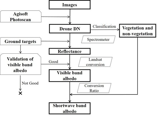
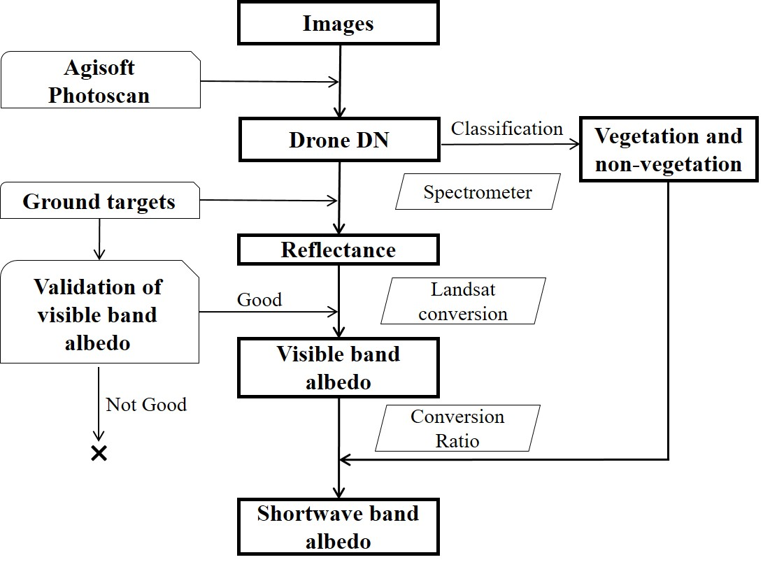
Figure 3 depicts the workflow of albedo estimation at the landscape scale. (i) A mosaicked image of the landscape was produced from the drone photographs using the Agisoft Photoscan software. (ii) The calibration functions based on the spectrometer measurement were used to convert the DN value of each pixel in the mosaicked image to spectral albedo in the three wavebands (red, green, and blue). (iii) The Landsat 8 visible band albedo algorithm (Equation (2) below) was validated with the visible band albedo of the ground targets. The validated Landsat 8 conversion algorithm was then used to determine the visible band albedo of each pixel in the whole image. The Landsat8 algorithm is given as [30]:
Here, α2, α3, and α4 represent blue, green, and red spectral albedos calculated from (ii), respectively. (iv) Pixels in the mosaicked image was classified as vegetation and non-vegetation types. (v) The shortwave albedo of the vegetation and non-vegetation pixels was obtained by multiplying their visible band albedo with the ratio of shortwave to visible band albedo obtained with the spectrometer for the vegetation ground targets and for the non-vegetation targets, respectively. (vi) The landscape shortwave albedo was calculated as the mean value of the pixels in the drone image mosaic. The visible and shortwave band albedo values were given as mean ± 1 standard deviation of all the pixel albedo values in the mosaic.
2.5. Retrieval of Landscape Albedo from the Landsat Satellite
Landsat 8 Operational Land Imager (OLI) surface reflectance products were used as a reference for evaluating the landscape visible and shortwave band albedo obtained with the drone images. These products have been atmospherically corrected from the Landsat 8 top of atmosphere reflectance by using the second simulation of the satellite signal in the Solar Spectrum Vectorial model [35]. They performed better than Landsat 5/7 products, by taking advantage of the new OLI coastal aerosol band (0.433–0.450 μm), which is beneficial for detecting aerosol properties [35]. The Landsat image was acquired on 6 October 2015 under clear sky condition and the WRS_PATH and Row were 13 and 31 respectively. The corresponding surface reflectance product can be ordered from https://earthexplorer.usgs.gov/. We used 72 pixels on the image that corresponded roughly to the drone image of the Brooksvale Park, and 16 pixels for the Yale Playground. The Landsat camera has a relatively small field of view (15°), and therefore, the BRDF correction is not considered in its surface reflectance product [36]. We used the Landsat 8 snow-free visible (Equation (2)) and shortwave band albedo coefficients (Equation (3)) to obtain the Landsat 8 validation values [30].
Here, α2, α3, α4, α5, α6, and α4 represent the spectral surface reflectances of six bands of Landsat 8 (450–510 nm, 530–590 nm, 640–670 nm, 850–880 nm, 1570–1650 nm, and 2110–2290 nm, respectively) [37]. Although it is possible to use the information retrieved from MODIS to make BRDF corrections to the Landsat albedo [29,30], this correction was not performed here, to be consistent with the drone methodology, which does not account for BRDF behaviors either.
3. Results
3.1. Relationship Between the DN Values and Spectral Reflectance
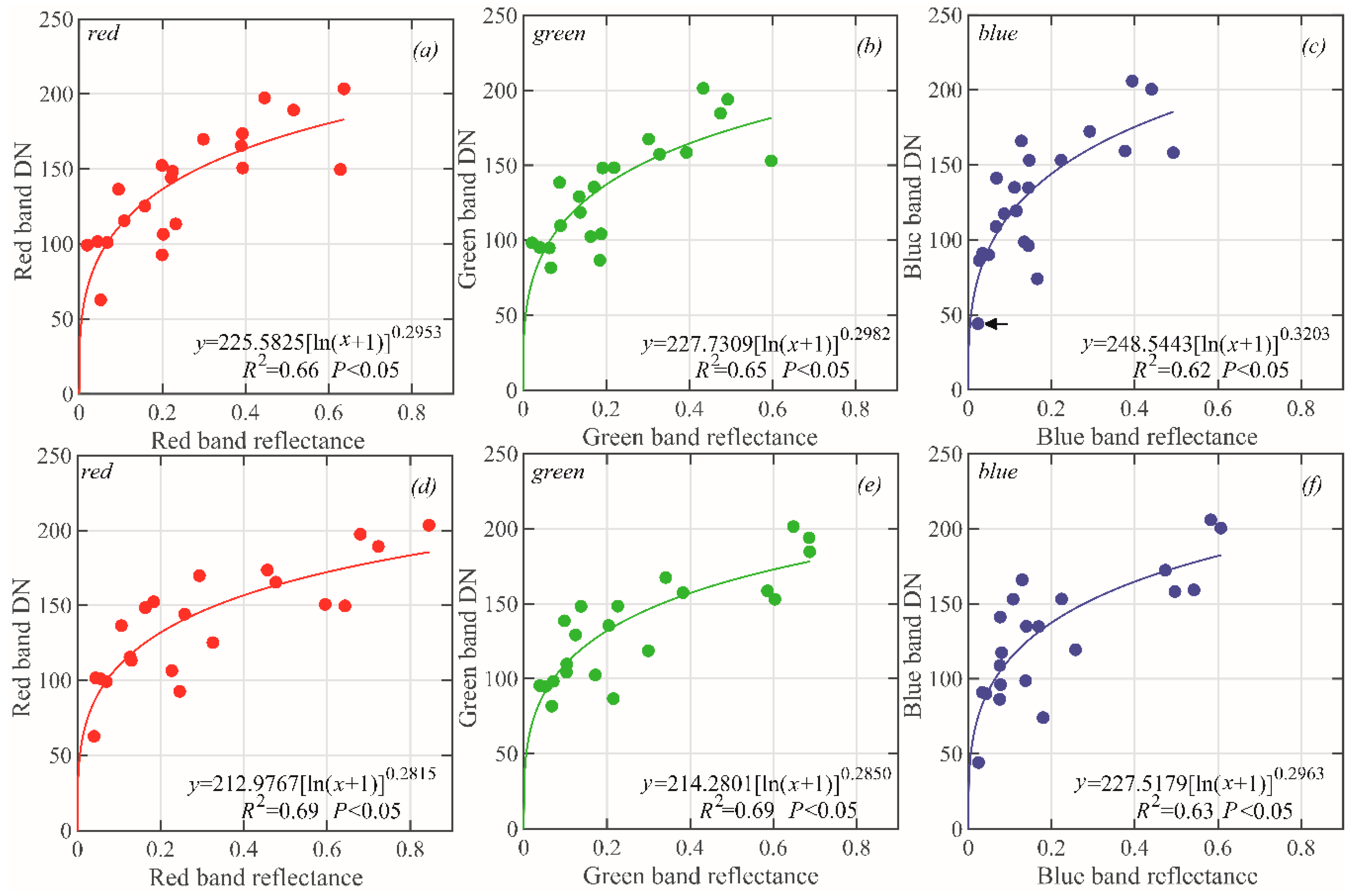
A desirable fitting function of the DN values and the spectral reflectance should meet two requirements: (1) when the reflectance reaches zero, the DN value should also reach zero, and (2) the relationship should be nonlinear because of gamma correction. In the study by Lebourgeois et al. [23], the relationship between the DN values in the raw and the compressed image format is logarithmic. Inspired by their result, we adopted the following fitting function for spectral calibration:
where x is the DN value of ground targets, y is spectral reflectance, and a and b are fitting coefficients. Equation (4) guarantees that the pixel reflectance is always positive.
y = a [ln(x + 1)] b
This function produced a robust regression fit to the spectral reflectance of the ground targets observed in the Brooksvale Park (Figure 4) and the Yale Playground (Figure 5). The coefficients of determination (R2) for Brooksvale Park were greater than 0.60 (p < 0.05) and those for the Yale Playground were greater than 0.40 (p < 0.05). For Brooksvale Park, all of the data points followed the fitting line closely. For the Yale Playground, there were two outliers: a yellow pavement mark, and a red brick (Figure 5). Such discrepancy may be indicative that these ground targets were not Lambertian reflectors. The view angle of the spectrometer was nadir. If the drone was relatively stable during the flight, the camera was levelled, and if only central pixels were used to form the mosaic, the camera angle would also be perfectly nadir. However, because the mosaic had pixels from other parts of the original photos, and because the camera position could deviate from the vertical, the actual camera angle viewing these targets may differ from the nadir. For this reason, a BRDF is required to correct for the non-Lamberstian behaviors, which is beyond the scope of this study.
3.2. Landscape Visible-Band and Shortwave Albedo
Applying the calibration functions (Figure 4d–f) obtained under overcast sky conditions to the pixels in Brooksvale Park, we obtained a landscape-level mean visible band albedo of 0.086 ± 0.110 (Table 3). The landscape visible band albedo of Yale Playground was 0.037 ± 0.063 according to the drone measurement. Here, the drone albedo was obtained using the clear-sky calibration functions (Figure 5a–c). The reader is reminded that the standard deviations here were computed from the albedo values of the pixels in the mosaics, and they therefore are indication of the variations across the landscapes, rather than uncertainties of our estimation.
The ratio of the shortwave to the visible band albedo of the non-vegetation and vegetation ground targets, are shown in Table 4. To estimate the shortwave albedo at the landscape scale, we first performed a classification of the mosaicked images. The results are illustrated in Figure S2. The vegetation and non-vegetation pixels occupied 61% and 39% of the land area in Brooksvale Park, respectively. Their visible band albedo values were multiplied by the conversion factors obtained for the vegetation and non-vegetation ground targets under overcast conditions, respectively, to obtain the shortwave albedo values. Averaging over the whole scene yielded a landscape shortwave albedo of 0.332 ± 0.527 under an overcast sky condition.
At the Yale Playground, a large portion of the pixels were in shadow, with low band reflectance. The spectral information in the three visible bands was insufficient for the classifier to identify which of these pixels were vegetation, and which were non-vegetation. Therefore for the Yale Playground, the image was divided into three classes: vegetation (25%), non-vegetation (50%), and shadow (25%). For the vegetation and non-vegetation pixels, the conversion factors obtained under clear sky conditions were used to estimate their shortwave albedo. For the pixels in shadow, the conversion factors obtained under overcast sky conditions were more appropriate. Since the pixels in shadows were not identifiable, we first assumed that all of them were vegetation (grass, SV), and by applying the conversion factor for vegetation (5.29), we arrived at an estimate of the landscape albedo of 0.061 ± 0.076. We then assumed that all of the pixels in shadows were non-vegetation (SN), obtaining a landscape albedo estimate of 0.054 ± 0.074. These two estimation did not differ by much. The actual albedo value of Yale Playground should fall between these two bounds.
4. Validation
4.1. Validation of LANDSAT Visible Band Albedo Conversion Algorithm
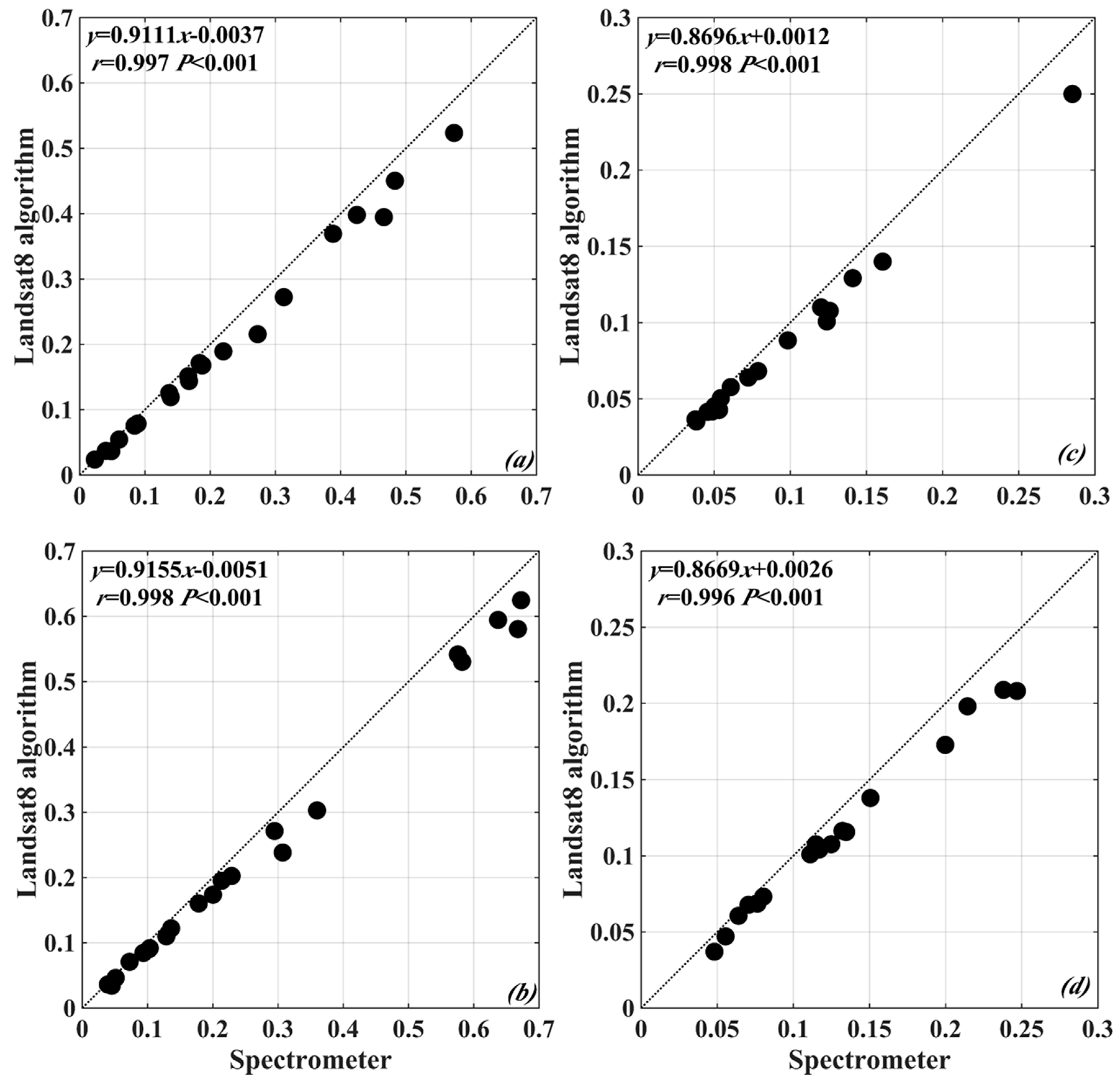
We used the spectrometer data to validate the Landsat albedo conversion algorithm (Equation (2)). As shown in Figure 6, the visible band albedo from the Landsat algorithm was highly correlated with the spectrometer measurement, with a linear correlation coefficient greater than 0.99, and a p value of less than 0.001. The mean bias error (Landsat minus spectrometer) was 0.01 under clear sky conditions. The linear correlation and the slope of the regression for the Yale Playground was slightly lower if the Landsat algorithm was applied to the band reference values obtained under overcast sky conditions (Figure 6d), but this was not a surprise because the Landsat algorithm was intended for clear skies.
The red, green, and blue bands defined for the ground targets were 620–670 nm, 540–560 nm, and 460–480 nm, respectively, in order to match those of the camera spectral sensitivity. These bands do not correspond precisely to the Landsat bands. Figure 6 shows that despite the slight mismatches, the Landsat algorithm can be used to convert camera-acquired reflectance to albedo.
4.2. Landscape Albedo Validation
For the Brooksvale Park, the drone-derived visible band albedo is 0.086 ± 0.110. For comparison, the Landsat visible band albedo is much lower, at 0.054 ± 0.0118. For the Yale Playground, the landscape visible band albedo was 0.037 ± 0.063 and 0.047 ± 0.012 according to the drone measurement and the Landsat measurement, respectively. Once again, because the standard deviations were computed from the individual pixel values in the scene for both the drone and the Landsat data, they indicated spatial variations of the albedo in the landscape, rather than uncertainties of estimation. The values of drone- and Landsat-derived visible band albedo for the Yale Playground were in much better agreement than those for the Brooksvale Park. We suggested that matching of sky conditions is the dominant factor for the different accuracies, as explained in the next section.
The Landsat-derived shortwave albedo is 0.103 ± 0.019 for the Brooksvale Park and 0.128 ± 0.013 for the Yale Playground. Compared with the landscape visible band albedo, the drone-derived shortwave albedo values (0.332 for Brooksvale Park and 0.054 to 0.061 for Yale Playground) are quite different from these reference values.
5. Discussion
5.1. Effect of Sky Conditions on Albedo Estimation
We conducted the spectrometer experiment under both clear sky and overcast sky conditions for the two drone field sites. The sky conditions had some effect on the regression statistics. The R2 values for Brooksvale Park were higher if the ground measurements were made under overcast sky conditions (Figure 4), the same conditions as when the UAV mission took place, than if the measurements were made under clear sky conditions. In contrast, R2 values for the Yale Playground were higher under clear sky conditions than under overcast sky conditions (Figure 5), keeping in mind that the UAV mission was conducted there under mostly clear sky conditions. These results indicate that the spectrometer calibration experiment should be conducted under the sky conditions that match those of the UAV experiment.
The Yale Playground flight was conducted at 14:30 on 30 September 2015 when the solar elevation angle was rather low. The long shadows due to the low elevation angle were a source of uncertainty for the albedo estimation. Choosing an appropriate flight time so that the shadow effect is minimized is very important, especially in an urban environment where tall structures are prominent features of the landscape.
The difference between the Landsat- and drone-derived visibleband albedo of the Brooksvale Park were larger than those of the Yale Playground. The main factor contributing to this discrepancy is also the sky condition. The UAV measurement was conducted under overcast conditions at Brooksvale Park, whereas the Landsat measurement was used for clear sky conditions. Generally, surface albedo is higher under cloudy skies than under clear skies [38]. At the Yale Playground, the sky conditions of the UAV experiment matched those of the Landsat observation, resulting in a much better agreement between the two albedo estimates.
5.2. Uncertainty in Landscape Shortwave Albedo
Low-cost consumer-grade cameras usually do not contain near-infrared spectral information, and therefore this may cause problems for estimating shortwave band albedo. In this study, shortwave band albedo was determined in a relatively arbitrary way. Brest and Goward [39] assigned weight factors to Landsat visible, near-infrared, and mid-infrared band reflectance, and linearly combined them to estimate the shortwave band albedo for vegetation. Similar to their method, we used the average ratio between the shortwave and visible band albedos of non-vegetation and vegetation ground targets to retrieve the landscape shortwave band albedo. The ratio for clear skies were lower than that for overcast skies for vegetation targets, suggesting that plants preferably absorb more visible radiation under clear skies than under overcast skies. For non-vegetation targets, the ratio did not differ by much between the two different sky conditions. Vegetation ground targets had higher ratios than the non-vegetation targets, due to the high near-infrared spectral reflectance of plant cell structures. The result from Brest’s [40] study may provide a useful reference here: They reported that urban downtown and high-density residential neighborhoods in Hartford, Connecticut, USA, had ratios of near-infrared to visible band reflectance between 1.29 and 1.38. Their ratio for evergreen and deciduous forests was between 2.53 and 3.63. From the shortwave and visible band albedos given in their study, we infer that their non-vegetation ratio of shortwave to visible band reflectance is 1.15 to 1.19, which is in good agreement with our non-vegetation ratios (1.18 to 1.24), and their vegetation (evergreen and deciduous trees) ratio is 1.77 to 2.32, which is much lower than our ratios (3.91 to 6.67). The main reason for the difference is that grass leaves (in this study the vegetation ground targets we chose was grass) have a higher spectral reflectance in the infrared waveband than tree leaves, which can increase shortwave albedo and therefore the ratio between shortwave and visible band reflectance [40].
Three modifications to our method can potentially improve the shortwave albedo accuracy. First, the addition of a light-weight NIRcamera can give a direct reflectance measurement to every ground pixel and therefore avoid the ratio method.
Second, in the current experiments, we were only able to perform a spectrometer measurement of the short grass targets. However, a large portion of the vegetation pixels are trees (Figure 2). Applying the NIR-to-visible band ratio obtained from the grass targets to these tree pixels will cause large errors. This is especially problematic for the Brooksvale Park where some trees started to become senescent (Figure 2a). Division of the vegetation pixels into three separate categories (grass, senescent tree leaf, and green tree leaf) and establishing the NIR to visible band for each category should improve the shortwave albedo accuracy.
Third, we deliberately selected the ground targets to cover a wide range of reflectivity to establish robust calibration curves, but we did not consider variations in BRDF signatures between grasses and trees, and between sands and tarmac. Currently only two training sets (vegetation versus non-vegetation) were used for conversions to shortwave albedo. Additional training sets accounting for BRDF variations may improve our results.
5.3. Potential Applications
Using cameras on-board a drone can provide timely estimation of the landscape albedo. For example, flying drone missions at different times of the day and season and in different weather and soil moisture conditions can provide information on the dynamic variations of albedo of the landscape. Such measurements may be especially useful in situations where monitoring with conventional radiometers is not feasible. For example, white roofs are proposed as a strategy to mitigate the urban heat island in the city landscape [41]. However, white paint on building roofs can suffer from erosion and dust deposition, and thus, its albedo can quickly decrease, from the original high values of 0.7 to 0.8 to values of 0.2 to 0.3 after a few years [42]. Direct measurement of roof albedo is challenging because roof spaces are generally not accessible by micrometeorological tower instruments. Drone flights conducted at different times can help to quantify the actual albedo and inform decisions on whether the roof needs cleaning or repainting. Another advantage of the drone methodology is its fine spatial resolution, as compared to satellite monitoring. Even with Sentinel 2 with a spatial resolution of 10 m, some landscape features (such as small fish ponds and small buildings) will become mixed satellite pixels.
6. Conclusions and Future Outlook
In this paper we tested a workflow for landscape albedo determination using images acquired by drone cameras. The key findings are as follows:
- (1)
- By adopting the method in this study, the landscape visible and shortwave band albedos of the Brooksvale Park were 0.086 and 0.332, respectively. For the Yale playground, the visible band albedo was 0.037, and shortwave albedo was between 0.054 and 0.061.
- (2)
- The Landsat satellite algorithm for converting the satellite spectral albedo to broadband albedo can also be used to convert spectral albedo that is acquired by drones to broadband albedo.
- (3)
- Data for spectral calibration using ground targets should be obtained under sky conditions that match those under which the drone flight take place. Because the relationship between the imagery DN value and the reflectivity is highly nonlinear, the ground targets should cover the range of reflectivity of the entire landscape.
- (4)
- In the current configuration, the drone estimate of the visible band albedo is more satisfactory than its estimate of shortwave albedo, when compared with the Landsat-derived values. We suggest that deployment of a camera with the additional capacity of measuring reflectance in a near-infrared waveband should improve the estimate of shortwave albedo. Future cameras with the capacity to detect mid-infrared reflectance will further improve the shortwave albedo detection. The BRDF effect, which was ignored in this study, should be taken into consideration when deciding the ground calibration targets and training data in future studies.
Supplementary Materials
The following are available online at https://0-www-mdpi-com.brum.beds.ac.uk/2072-4292/10/11/1812/s1, Figure S1: Pictures of some of the selected ground targets for Brooksvale Park and Yale Playground, Figure S2: Classification of the mosaicked image for Brooksvale Park (a) and Yale Playground (b), Figure S3: Visible (a), shortwave band albedo for the Yale Playground when all shadow were taken as non-vegetation (b) and vegetation (c) under clear sky conditions, Figure S4: Visible (a) and shortwave band albedo (b) for the Brooksvale Park under clear sky conditions, Figure S5: Landsat visible (a) and shortwave band albedo (b) for the Yale Playground, Figure S6: Landsat visible (a) and shortwave band albedo (b) for the Brooksvale Park, Table S1: Input parameters for the SMART model.
Author Contributions
Conceptualization, X.L. and C.C.; Methodology, J.M., N.T., G.T., C.C., J.X., and L.B.; Formal Analysis, C.C.; Writing—Original Draft Preparation, C.C.; Writing—Review & Editing, X.L.
Funding
This research was funded by the Startup Foundation for Introducing Talent of Nanjing University of Information Science and Technology (grant 2017r067), Natural Science Foundation of Jiangsu Province (grants BK20180796 BK20181100), National Natural Science Foundation of China (grant 41805022), the Ministry of Education of China (grant PCSIRT), the Priority Academic Program Development of Jiangsu Higher Education Institutions (grant PAPD), and a Visiting Fellowship from China Scholarship Council (to C.C.).
Acknowledgments
We would like to thank Nina Kantcheva Tushev and Georgi Tushev for their help in conducting the drone experiment at the Yale Playground.
Conflicts of Interest
The authors declare no conflict of interest.
References
- Liang, S. Narrowband to broadband conversions of land surface albedo I: Algorithms. Remote Sens. Environ. 2001, 76, 213–238. [Google Scholar] [CrossRef]
- Hock, R. Glacier melt: A review of processes and their modelling. Prog. Phys. Geogr. 2005, 29, 362–391. [Google Scholar] [CrossRef]
- Jin, Y.; Schaaf, C.B.; Gao, F.; Li, X.; Strahler, A.H.; Zeng, X.; Dickinson, R.E. How does snow impact the albedo of vegetated land surfaces as analyzed with MODIS data? Geophys. Res. Lett. 2002, 29, 1374. [Google Scholar] [CrossRef]
- Myhre, G.; Kvalevåg, M.M.; Schaaf, C.B. Radiative forcing due to anthropogenic vegetation change based on MODIS surface albedo data. Geophys. Res. Lett. 2005, 32, L21410. [Google Scholar] [CrossRef]
- Jin, Y.; Randerson, J.T.; Goetz, S.J.; Beck, P.S.; Loranty, M.M.; Goulden, M.L. The influence of burn severity on postfire vegetation recovery and albedo change during early succession in North American boreal forests. J. Geophys. Res. Biogeosci. 2012, 117, G01036. [Google Scholar] [CrossRef]
- Cescatti, A.; Marcolla, B.; Vannan, S.K.; Pan, J.Y.; Román, M.O.; Yang, X.; Ciais, P.; Cook, R.B.; Law, B.E.; Matteucci, G.; et al. Intercomparison of MODIS albedo retrievals and in situ measurements across the global FLUXNET network. Remote Sens. Environ. 2012, 121, 323–334. [Google Scholar] [CrossRef] [Green Version]
- Fernández, T.; Pérez, J.L.; Cardenal, J.; Gómez, J.M.; Colomo, C.; Delgado, J. Analysis of landslide evolution affecting olive groves using UAV and photogrammetric techniques. Remote Sens. 2016, 8, 837. [Google Scholar] [CrossRef]
- Watts, A.C.; Ambrosia, V.G.; Hinkley, E.A. Unmanned aircraft systems in remote sensing and scientific research: Classification and consideration of use. Remote Sens. 2012, 4, 1671–1692. [Google Scholar] [CrossRef]
- Salamí, E.; Barrado, C.; Pastor, E. UAV flight experiments applied to the remote sensing of vegetated areas. Remote Sens. 2014, 6, 11051–11081. [Google Scholar] [CrossRef] [Green Version]
- Nex, F.; Remondino, F. UAV for 3D mapping applications: A review. Appl. Geomat. 2014, 6, 1–15. [Google Scholar] [CrossRef]
- Laliberte, A.S.; Goforth, M.A.; Steele, C.M.; Rango, A. Multispectral remote sensing from unmanned aircraft: Image processing workflows and applications for rangeland environments. Remote Sens. 2011, 3, 2529–2551. [Google Scholar] [CrossRef]
- Stolaroff, J.K.; Samaras, C.; O’Neill, E.R.; Lubers, A.; Mitchell, A.S.; Ceperley, D. Energy use and life cycle greenhouse gas emissions of drones for commercial package delivery. Nat. Commun. 2018, 9, 409. [Google Scholar] [CrossRef] [PubMed]
- Yang, G.; Li, C.; Wang, Y.; Yuan, H.; Feng, H.; Xu, B.; Yang, X. The DOM generation and precise radiometric calibration of a UAV-mounted miniature snapshot hyperspectral imager. Remote Sens. 2017, 9, 642. [Google Scholar] [CrossRef]
- Sonnentag, O.; Hufkens, K.; Teshera-Sterne, C.; Young, A.M.; Friedl, M.; Braswell, B.H.; Milliman, T.; O’Keefe, J.; Richardson, A.D. Digital repeat photography for phenological research in forest ecosystems. Agric. For. Meteorol. 2012, 152, 159–177. [Google Scholar] [CrossRef]
- Saari, H.; Pellikka, I.; Pesonen, L.; Tuominen, S.; Heikkilä, J.; Holmlnd, C.; Mäkynen, J.; Ojala, K.; Antila, T. Unmanned Aerial Vehicle (UAV) operated spectral camera system for forest and agriculture applications. Proc. SPIE 2011, 8174, 466–471. [Google Scholar]
- Johnson, L.F.; Herwitz, S.; Dunagan, S.; Lobitz, B.; Sullivan, D.; Slye, R. Collection of ultra high spatial and spectral resolution image data over California vineyards with a small UAV. In Proceedings of the International Symposium on Remote Sensing of Environment, Beijing, China, 22–26 April 2003. [Google Scholar]
- Berni, J.A.J.; Suárez, L.; Fereres, E. Remote Sensing of Vegetation from UAV Platforms Using Lightweight Multispectral and Thermal Imaging Sensors. Available online: http://www.isprs.org/proceedings/XXXVIII/1_4_7-W5/paper/Jimenez_Berni-155.pdf (accessed on 21 March 2016).
- Zahawi, R.A.; Dandois, J.P.; Holl, K.D.; Nadwodny, D.; Reid, J.L.; Ellis, E.C. Using lightweight unmanned aerial vehicles to monitor tropical forest recovery. Biol. Conserv. 2015, 186, 287–295. [Google Scholar] [CrossRef] [Green Version]
- Bendig, J.; Yu, K.; Aasen, H.; Bolten, A.; Bennertz, S.; Broscheit, J.; Gnyp, M.L.; Bareth, G. Combining UAV-based plant height from crop surface models, visible, and near infrared vegetation indices for biomass monitoring in barley. Int. J. Appl. Earth Obs. 2015, 39, 79–87. [Google Scholar] [CrossRef]
- Levy, C.; Burakowski, E.; Richardson, A. Novel measurements of fine-scale albedo: Using a commercial quadcopter to measure radiation fluxes. Remote Sens. 2018, 10, 1303. [Google Scholar] [CrossRef]
- Hakala, T.; Suomalainen, J.; Peltoniemi, J.I. Acquisition of Bidirectional Reflectance Factor Dataset Using a Micro Unmanned Aerial Vehicle and a Consumer Camera. Remote Sens. 2010, 2, 819–832. [Google Scholar] [CrossRef] [Green Version]
- Ryan, J.; Hubbard, A.; Box, J.E.; Brough, S.; Cameron, K.; Cook, J.; Cooper, M.; Doyle, S.H.; Edwards, A.; Holt, T.; et al. Derivation of High Spatial Resolution Albedo from UAV Digital Imagery: Application over the Greenland Ice Sheet. Front. Earth Sci. 2017, 5. [Google Scholar] [CrossRef] [Green Version]
- Lebourgeois, V.; Bégué, A.; Labbé, S.; Mallavan, L.; Prévost, B.R. Can Commercial Digital Cameras Be Used as Multispectral Sensors? A Crop Monitoring Test. Sensors 2008, 8, 7300–7322. [Google Scholar] [CrossRef] [PubMed] [Green Version]
- Lelong, C.C.D.; Burger, P.; Jubelin, G.; Roux, B.; Labbé, S.; Baret, F. Assessment of Unmanned Aerial Vehicles Imagery for Quantitative Monitoring of Wheat Crop in Small Plots. Sensors 2008, 8, 3557–3585. [Google Scholar] [CrossRef] [PubMed] [Green Version]
- Markelin, L.; Honkavaara, E.; Peltoniemi, J.; Ahokas, E.; Kuittinen, R.; Hyyppä, J.; Suomalainen, J.; Kukko, A. Radiometric Calibration and Characterization of Large-format Digital Photogrammetric Sensors in a Test Field. Photogramm. Eng. Remote Sens. 2008, 74, 1487–1500. [Google Scholar] [CrossRef]
- Honkavaara, E.; Arbiol, R.; Markelin, L.; Martinez, L.; Cramer, M.; Bovet, S.; Chandelier, L.; Ilves, R.; Klonus, S.; Marshal, P.; et al. Digital Airborne Photogrammetry—A New Tool for quantitative remote sensing? A State-of-Art review on Radiometric Aspects of Digital Photogrammetric Images. Remote Sens. 2009, 1, 577–605. [Google Scholar] [CrossRef] [Green Version]
- Du, M.; Noguchi, N. Monitoring of Wheat Growth Status and Mapping of Wheat Yield’s within-Field Spatial Variations Using Color Images Acquired from UAV-camera System. Remote Sens. 2017, 9, 289. [Google Scholar] [CrossRef]
- Wang, M.; Chen, C.; Pan, J.; Zhu, Y.; Chang, X. A Relative Radiometric Calibration Method Based on the Histogram of Side-Slither Data for High-Resolution Optical Satellite Imagery. Remote Sens. 2018, 10, 381. [Google Scholar] [CrossRef]
- Shuai, Y.; Masek, J.; Gao, F.; Schaaf, C. An algorithm for the retrieval of 30-m snow-free albedo from Landsat surface reflectance and MODIS BRDF. Remote Sens. Environ. 2011, 115, 2204–2216. [Google Scholar] [CrossRef]
- Wang, Z.; Erb, A.M.; Schaaf, C.B.; Sun, Q.; Liu, Y.; Yang, Y.; Shuai, Y.; Casey, K.A.; Roman, M.O. Early spring post-fire snow albedo dynamics in high latitude boreal forests using Landsat-8 OLI data. Remote Sens. Environ. 2016, 185, 71–83. [Google Scholar] [CrossRef] [PubMed] [Green Version]
- Available online: http://www.cielmap.com/cielmap/ (accessed on 28 June 2016).
- Agisoft Photoscan User Manual. Available online: http://www.agisoft.com/pdf/photoscan-pro_1_2_en.pdf/ (accessed on 18 July 2016).
- Kruse, F.A.; Lefkoff, A.B.; Boardman, J.W.; Heidebrecht, K.B.; Shapiro, A.T.; Barloon, P.J.; Goetz, A.F.H. The spectral image processing system (SIPS)—Interactive visualization and analysis of imaging spectrometer data. Remote Sens. Environ. 1993, 44, 145–163. [Google Scholar] [CrossRef]
- Gueymard, C.A. The sun’s total and spectral irradiance for solar energy applications and solar radiation models. Sol. Energy 2004, 76, 423–453. [Google Scholar] [CrossRef]
- He, T.; Liang, S.; Wang, D.; Cao, Y.; Gao, F.; Yu, Y.; Feng, M. Evaluating land surface albedo estimation from Landsat MSS, TM, ETM+, and OLI data based on the unified direct estimation approach. Remote Sens. Environ. 2018, 204, 181–196. [Google Scholar] [CrossRef]
- Landsat8 Surface Reflectance Code (LaSRC) Product Guide. Available online: https://landsat.usgs.gov/sites/default/files/documents/lasrc_product_guide.pdf (accessed on 14 February 2018).
- Vermote, E.; Justice, C.; Claverie, M.; Franch, B. Preliminary analysis of the performance of the Landsat 8/OLI land surface reflectance product. Remote Sens. Environ. 2016, 185, 46–56. [Google Scholar] [CrossRef]
- Payne, R.E. Albedo of the sea surface. J. Atmos. Sci. 1972, 29, 959–970. [Google Scholar] [CrossRef]
- Brest, C.; Goward, S. Deriving surface albedo measurements from narrow band satellite data. Int. J. Remote Sens. 1987, 8, 351–367. [Google Scholar] [CrossRef]
- Brest, C. Seasonal albedo of an urban/rural landscape from satellite observations. J. Clim. Appl. Meteorol. 1987, 26, 1169–1187. [Google Scholar] [CrossRef]
- Zhao, L.; Lee, X.; Schultz, M. A wedge strategy for mitigation of urban warming in future climate scenarios. Atmos. Chem. Phys. 2017, 17, 9067–9080. [Google Scholar] [CrossRef] [Green Version]
- Akbari, H.; Kolokotsa, D. Three decades of urban heat islands and mitigation technologies research. Energy Build. 2016, 133, 834–842. [Google Scholar] [CrossRef]
Figure 1.
The unmanned aerial vehicles (UAVs) before launch. (a,b) are the fixed-wing and rotor wing UAVs for Brooksvale Park and Yale Playground, respectively.
Figure 1.
The unmanned aerial vehicles (UAVs) before launch. (a,b) are the fixed-wing and rotor wing UAVs for Brooksvale Park and Yale Playground, respectively.

Figure 2.
Mosaicked images of Brooksvale Park (a) and Yale Playground (b). The mosaicked images have a resolution of 4 cm per pixel.
Figure 2.
Mosaicked images of Brooksvale Park (a) and Yale Playground (b). The mosaicked images have a resolution of 4 cm per pixel.

Figure 3.
Workflow for estimating landscape visible and shortwave band albedo.

Figure 4.
Regression fit between the band DN value and band reflectance of ground targets in Brooksvale Park. Panels (a–c) are for clear sky conditions, and (d–f) are for overcast sky conditions under which the spectrometer measurement took place. Also shown are the regression equation, coefficient of determination (R2), and the confidence level (p).

Figure 5.
The description is the same as in Figure 4 except for the location being Yale Playground. Arrows indicate outliers discussed in the text.
Figure 5.
The description is the same as in Figure 4 except for the location being Yale Playground. Arrows indicate outliers discussed in the text.

Figure 6.
Comparison of visible band albedo measured with the spectrometer and derived with the Landsat conversion algorithm for the Brooksvale Park (a,b) and the Yale Playground (c,d). Panels (a,c) are for clear sky conditions and (b,d) are for overcast sky conditions.
Figure 6.
Comparison of visible band albedo measured with the spectrometer and derived with the Landsat conversion algorithm for the Brooksvale Park (a,b) and the Yale Playground (c,d). Panels (a,c) are for clear sky conditions and (b,d) are for overcast sky conditions.


Table 1.
Information about the study sites and the drone experiments. Here, image overlap is defined as the number of photos that were sampled in the same pixel. For example, an overlap of nine means that each pixel is seen by at least nine photos.
Table 1.
Information about the study sites and the drone experiments. Here, image overlap is defined as the number of photos that were sampled in the same pixel. For example, an overlap of nine means that each pixel is seen by at least nine photos.
| Brooksvale Recreation Park | Yale Playground | |
|---|---|---|
| Location | 41.453°N 72.918°W | 41.317°N 72.928°W |
| Drone experiment date | 9 October 2015 | 30 September 2015 |
| Drone flight time | 10:00 to 10:30 | 14:30 to 15:00 |
| Sky conditions | Overcast | Clear sky |
| Flight duration | 30 min | 20 min |
| Flight altitude (m) | 120 | 90 |
| Camera | Sony NEX-5N | GARMIN VIRB-X |
| UAV platform | Fixed-wing | Quad-rotor |
| Forward overlap | 80% | 80% |
| Side overlap | 60% | 60% |
| Image overlap Area (km2) | >9 0.065 | >9 0.014 |
Table 2.
Dates of the spectrometer field experiments.
| Sky Conditions | Brooksvale Park | Yale Playground |
|---|---|---|
| Clear | 28 April 2016 10:00 | 19 April 2016 14:30 |
| Overcast | 7 March 2016 10:00 | 28 April 2016 14:30 |
Table 3.
Comparison of drone-derived and Landsat 8 visible and shortwave band albedo under clear and overcast sky conditions for the Brooksvale Park and the Yale Playground. Refer to Supplementary Figures S3–S6 for the spatial distributions of these albedo values.
Table 3.
Comparison of drone-derived and Landsat 8 visible and shortwave band albedo under clear and overcast sky conditions for the Brooksvale Park and the Yale Playground. Refer to Supplementary Figures S3–S6 for the spatial distributions of these albedo values.
| Brooksvale Park | Yale Playground | |
|---|---|---|
| Drone-derived visible band albedo | c: 0.077 ± 0.091 | c: 0.037 ± 0.063 |
| o: 0.086 ± 0.110 | o: 0.054 ± 0.090 | |
| Landsat 8 visible band albedo | 0.054 ± 0.011 | 0.047 ± 0.012 |
| Drone-derived shortwave band albedo | c: 0.261 ± 0.395 | SN: 0.054 ± 0.074 |
| o: 0.332 ± 0.527 | SV: 0.061 ± 0.076 | |
| Landsat 8 shortwave band albedo | 0.103 ± 0.019 | 0.128 ± 0.013 |
c and o represent clear and overcast sky conditions, respectively; SN and SV represent that the shadow on the Yale Playground were taken as non-vegetation and vegetation, respectively.
Table 4.
Ratio between the shortwave and visible band albedo obtained with the spectrometer for the vegetation and non-vegetation targets of the Brooksvale Park and the Yale Playground.
Table 4.
Ratio between the shortwave and visible band albedo obtained with the spectrometer for the vegetation and non-vegetation targets of the Brooksvale Park and the Yale Playground.
| Sky Condition | Brooksvale Park | Yale Playground | ||
|---|---|---|---|---|
| Vegetation | Non-Vegetation | Vegetation | Non-Vegetation | |
| Clear | 5.08 | 1.18 | 3.91 | 1.24 |
| Overcast | 6.76 | 1.20 | 5.29 | 1.18 |
© 2018 by the authors. Licensee MDPI, Basel, Switzerland. This article is an open access article distributed under the terms and conditions of the Creative Commons Attribution (CC BY) license (http://creativecommons.org/licenses/by/4.0/).
Share and Cite
MDPI and ACS Style
Cao, C.; Lee, X.; Muhlhausen, J.; Bonneau, L.; Xu, J. Measuring Landscape Albedo Using Unmanned Aerial Vehicles. Remote Sens. 2018, 10, 1812. https://0-doi-org.brum.beds.ac.uk/10.3390/rs10111812
AMA Style
Cao C, Lee X, Muhlhausen J, Bonneau L, Xu J. Measuring Landscape Albedo Using Unmanned Aerial Vehicles. Remote Sensing. 2018; 10(11):1812. https://0-doi-org.brum.beds.ac.uk/10.3390/rs10111812
Chicago/Turabian StyleCao, Chang, Xuhui Lee, Joseph Muhlhausen, Laurent Bonneau, and Jiaping Xu. 2018. "Measuring Landscape Albedo Using Unmanned Aerial Vehicles" Remote Sensing 10, no. 11: 1812. https://0-doi-org.brum.beds.ac.uk/10.3390/rs10111812
Note that from the first issue of 2016, this journal uses article numbers instead of page numbers. See further details here.