Infrared Small Target Detection via Non-Convex Rank Approximation Minimization Joint l_2,1 Norm

Abstract

To improve the detection ability of infrared small targets in complex backgrounds, a novel method based on non-convex rank approximation minimization joint l_2,1 norm (NRAM) was proposed. Due to the defects of the nuclear norm and l₁ norm, the state-of-the-art infrared image-patch (IPI) model usually leaves background residuals in the target image. To fix this problem, a non-convex, tighter rank surrogate and weighted l₁ norm are instead utilized, which can suppress the background better while preserving the target efficiently. Considering that many state-of-the-art methods are still unable to fully suppress sparse strong edges, the structured l_2,1 norm was introduced to wipe out the strong residuals. Furthermore, with the help of exploiting the structured norm and tighter rank surrogate, the proposed model was more robust when facing various complex or blurry scenes. To solve this non-convex model, an efficient optimization algorithm based on alternating direction method of multipliers (ADMM) plus difference of convex (DC) programming was designed. Extensive experimental results illustrate that the proposed method not only shows superiority in background suppression and target enhancement, but also reduces the computational complexity compared with other baselines.

1. Introduction

Infrared search and track (IRST) systems have been widely used in many applications, especially in the military field. As a basic function of IRST systems, infrared small target detection plays an important role in early-warning, precision guidance, and long-range target detection. However, the lack of texture and structure information of the target under infrared conditions, coupled with the influence of long distance, complex background, and various clutter, means that the infrared small target is often spot-like, even submerged in the background, which makes it extremely difficult to detect. Therefore, it is a challenge to design a detection method that is effective and adaptable to various complex backgrounds.

Generally speaking, infrared small target detection methods can be divided into two categories: sequential-based and single-frame-based methods. Sequential-based methods need to join multiple frames to capture the target trajectory and avoid noise interference. When the background is homogeneous and the target moves slowly, sequential-based methods such as the Robinson Guard spatial filter [1], dynamic programming algorithm [2], 3D matched filtering [3], and so on can perform well. Nevertheless, in real applications, not only is it difficult to guarantee the homogeneity of the background, but the movement between the target and imaging sensor is fast, resulting in the rapid degrading of sequential-based methods. Meanwhile, high storage and hardware requirements make this approach unsuitable for large-scale engineering projects. Although there are still some studies on sequential methods [4,5], single-frame based methods are more popular and have attracted more research attention in recent years [6,7,8].

Conventional single-frame based detection approaches, like Tophat filter [9], Maxmean and Maxmedian filter [10] utilize filtering to suppress the background and enhance the target under the assumption of background consistency. These methods can achieve good performance with a uniform background and are easily implemented. Unfortunately, most backgrounds do not meet the ideal assumption, leading to a high false alarm ratio. Recently, approaches based on human visual system (HVS) [11] have been developed to improve the performance of infrared small target detection with the assumption that the target is the most salient object, most of which compute the saliency map in a manner of filtering [7,12,13,14,15,16,17,18] or transforming [19,20]. Actually, in many real scenes, the most prominent object is not the desired target while the highlight edges and salient non-target components can destroy the whole detection. Both of these methods are sensitive to noise and do not perform well when the size of the target varies within a large range.

Conventional detection methods based on simple assumptions merely consider either the background or the target. In order to overcome the limitations of the traditional methods, a state-of-the-art approach based on robust principal component analysis (RPCA) called the infrared patch-image (IPI) model was proposed [21]. Focusing on the non-local self-correlation configuration of the background, the assumption of the IPI model fits real scenes well. Unlike the general infrared image model, the IPI model reformulates it as follows:

$$D=B+T+N$$

(1)

where D, B, T, and N are the corresponding patch-images of the original infrared image, the background image, the target image, and the random noise image, respectively. Then, with the low-rank property of B and the sparsity of T, the conventional small target detection problem is converted to a RPCA optimization problem (RPCA is also called sparse and low rank matrix decomposition) as follows:

$$\begin{array}{l}\underset{B,T}{\min }{\Vert B\Vert }_{\ast }+\lambda {\Vert T\Vert }_1\\ \mathrm{s}.\mathrm{t}.D=B+T\end{array}$$

(2)

where ${\Vert •\Vert }_{\ast }$ denotes the nuclear norm of a matrix (i.e., the sum of singular values), ${\Vert •\Vert }_1$ is the l₁ norm (i.e., ${\Vert X\Vert }_1={\displaystyle {\sum }_{ij}\left|X_{ij}\right|}$), and λ is a positive weighting constant.

Convex problem (2) is efficiently solved in Reference [21] via the accelerated proximal gradient (APG) [22] approach. However, since nuclear norm minimization (NNM) treats all singular values equally, it may obtain suboptimal solutions [23]. The l₁ norm faces the same problem, which means that Equation (2) cannot recover the background and target image precisely. In other words, when facing complex infrared scenes, the performance of IPI is weak, namely, strong edge residuals remain in the recovered target image and the recovered background is blurry (poor edge retention). To approximate the rank more accurately, many non-convex surrogates have been introduced to RPCA one after another because of their flexibility including weighted nuclear norm minimization (WNNM) [24], truncated nuclear norm minimization (TNNM) [25], capped norm [26], the Schatten-p norm [27] and so forth. Similarly, weighted l₁ norm [28], capped l₁ norm [29], and l_2,1 norm [30] have also been proposed to improve the ability to represent sparsity.

Furthermore, alternating direction method of multipliers (ADMM) [31] has a faster convergence rate when compared with APG and its precision is also higher [32]. Hence, ADMM is a popular method to solve optimization problems in many fields, particularly in the computer vision and image processing field. For instance, Gu et al. [33] utilized ADMM to solve the non-convex weighted nuclear norm minimization (WNNM) problem efficiently, which was successfully applied to image inpainting. Xue et al. [34] proposed a non-convex low-rank tensor completion model using ADMM to obtain the best recovery result in color images. Based on total variation regularized tensor RPCA, Cao et al. [35] designed a non-convex and non-separable model to complete background subtraction with an ADMM solver.

In this paper, a novel approach based on non-convex rank approximation minimization (NRAM) joint l_2,1 norm was proposed to overcome the deficiencies of Equation (2). Additionally, a more accurate weighted l₁ norm was introduced to better depict the target component. By incorporating the structured sparse item, the strong non-target component, particularly borders, could be wiped out. To solve this non-convex optimization problem, a method using alternating direction method of multipliers (ADMM) plus difference of convex (DC) programming [36] is presented, which has a lower computation complexity.

The remainder of this paper is organized as follows. In Section 2, we give an overview of related works on infrared small target detection and briefly analyze the common existing problems. The proposed NRAM model is presented in Section 3. In Section 4, extensive experiments on various scenes and sequences are conducted to illustrate the efficiency of the proposed method. Analysis and comparisons are also given. A discussion and conclusions are presented in Section 5 and Section 6, respectively.

2. Related Works

Many algorithms have been proposed for infrared small target detection. The existing single-frame-based detection algorithms mainly fall into three main groups: methods of background-based assumption, methods of target-based assumption, and methods of target and background separating.

2.1. Methods of Background-Based Assumption

These methods utilize filtering to estimate the background under the assumption of background consistency. When the estimation is conducted, the target is enhanced by subtracting the background from the original image. Obviously, the selection of filters directly affects the accuracy of the detection. Tophat filter [9], Maxmean filter and Maxmedian filter [10] are three typical filters used in this detection field. By selecting different structural elements or sliding windows, targets can be caught easily in simple uniform scenes in real-time. In addition, the two-dimensional least mean square (TDLMS) filter [37] can automatically estimate the background by adaptive iteration with strong robustness compared with the above three filtering-based methods, yet does not perform in real-time. Subsequently, some improved methods, like the bilateral TDLMS (BTDLMS) filter [38], edge directional TDLMS (EDTDLMS) filter [39], and novel TDLMS filter [40] have been proposed for the sake of better performance. Unfortunately, they work well only if the background meets the simple assumption. Once the input infrared image becomes complex, the obtained residual image is frequently full of noise and background disturbance, leading to a huge challenge in identifying the true targets in post-processing. When considering complex input, they cannot handle strong target-like edges and, in fact, regard the edges as targets.

2.2. Methods of Target-Based Assumption

In recent years, human visual system (HVS) [11] with properties including size-adaptation, contrast mechanisms, and attention shift mechanisms have been developed to improve the performance of infrared small target detection with the assumption that the target is the most salient object. By means of filtering or transforming, the saliency map is calculated to make true targets as salient as possible, most of which are based on a single contrast mechanism such as the Laplacian of Gaussian (LoG) filter [12], and the difference of Gaussian (DoG) filter [13]. Obviously, how to define the contrast between the target and background is one of the key steps for HVS-based methods. The local contrast measure (LCM) [14] was first proposed to describe the dissimilarity between the current cell and its eight adjacent cells, which is calculated pixel by pixel and is very time consuming. For good performance in detection rate, false alarm rate and speed simultaneously, the improved LCM (ILCM) [15], the novel LCM (NLCM) [16], and the relative LCM (RLCM) [17] were provided to calculate the saliency map. The multiscale patch-based contrast measure (MPCM) [18] focuses on the multi-directional dissimilarity between the current patch and the surrounding patches. To improve the performance of MPCM, Li et al. [41] extended it to a speed-up version, and exploited density clustering to reduce the false alarm rate. From another perspective, Li et al. [19] and Tang et al. [20] analyzed visual saliency in the frequency domain. On the whole, HSV-based methods are sensitive to edges while the small targets fail to meet the requirements of the above assumption.

2.3. Methods of Target and Background Separating

Apart from concentrating merely on the single background or target, some recent methods can separate the target and background simultaneously. The typical approach, IPI [21] utilizes the non-local self-correlation of infrared background and the sparsity of the target to reveal the data structure, and experimental results show an obvious superiority when compared with the traditional methods. However, it is time consuming. Dai et al. [42] pointed out that IPI would either over-shrink the small targets or leave some residuals in the target image because of the limitation of the l₁ norm and fixed constant weighting parameter. To address such problems, the authors proposed a weighted IPI (WIPI) model via the column-wise weights. Focusing on the defect of the nuclear norm that leads to background residuals in the target image, Dai et al. [43] analyzed the reason for the remaining residuals resulting from the mismatching of the IPI model’s implicit assumption of a large amount of observations with the reality of deficient observations of strong cloud edges, and developed NIPPS exploiting partial sum minimization of singular values (PSSV) [44] to preserve the large singular values related to the observed noise data, not the whole input matrix. However, the accuracy of NIPPS depends on estimating the rank of the background matrix, whose performance degrades when facing complex backgrounds. ReWIPI [28] combines WNNM and the weighted l₁ norm to restrain low rank and sparsity, penalizing the larger singular values by smaller weights, so that the non-target sparse points could be efficiently suppressed.

Considering the fact that the original data were drawn from a union of low-rank subspaces, low-rank representation (LRR) [45] is used to recover background and target by a self-expressive dictionary with low-rank coefficients and the sparse noise. Based on LRR, low-rank and sparse representation (LRSR) [30] has been proposed, which adds the sparse representation of the special structure into the LRR with two additional input dictionaries. Liu et al. [46] utilized fractal background over-complete dictionary (FBOD) and generalized Gaussian target over-complete dictionary (GGTOD) together to suppress the heavy sky clutter in infrared images. Note that the projection onto the dictionary is applied to every overlapped patch, which takes lots of time, and it is difficult to generate the appropriate dictionaries. From another perspective, Wang et al. [47] presented a method named the stable multisubspace learning (SMSL) method that took into account the inner structure of actual images in heterogeneous scenes. Moreover, compared with IPI-based methods in general, multisubspace-based methods do not show superiority in terms of performance. To better recognize strong edges, Dai et al. [48] introduced structure tensor into a reweighted infrared patch-tensor model (RIPT), employing both the local and nonlocal priors. Nevertheless, it does not work well when the targets are close to or on the boundaries, leaving much noise. Worse still, this approach breaks down when the target is not sufficiently salient.

Table 1. Characteristics of typical methods based on target and background separation.

Methods	Advantages	Disadvantages
IPI	Works well with uniform scenes.	Over-shrinks the small targets, leaving residuals in the target image, time consuming.
NIPPS	Works well when strong edges and non-target interferences are few.	Difficult to estimate rank of data, fails to eliminate strong edges and non-target interference.
ReWIPI	Works well when background changes slowly.	Sensitive to rare highlight borders, performance degrading with the increasing of complexity.
LRR	Works well with simple scenes.	Cannot handle complex backgrounds.
LRSR	Works well with homogeneous backgrounds.	Difficult to choose two dictionaries simultaneously, leaving noise in target component.
FBOD + GGTOD	Work well with sky background clutter.	Difficult to choose two dictionaries simultaneously, cannot handle other scenes well.
SMSL	Works well when the target is salient and the background is clean.	Sensitive to boundaries, poor at background suppression, loses target easily.
RIPT	Works well when the target is salient.	Does not work well when the targets are close to or on the boundaries, leaving much noise, loses target totally when target is not sufficiently salient.

below shows a summary of the common approaches based on the separation of background and target image.

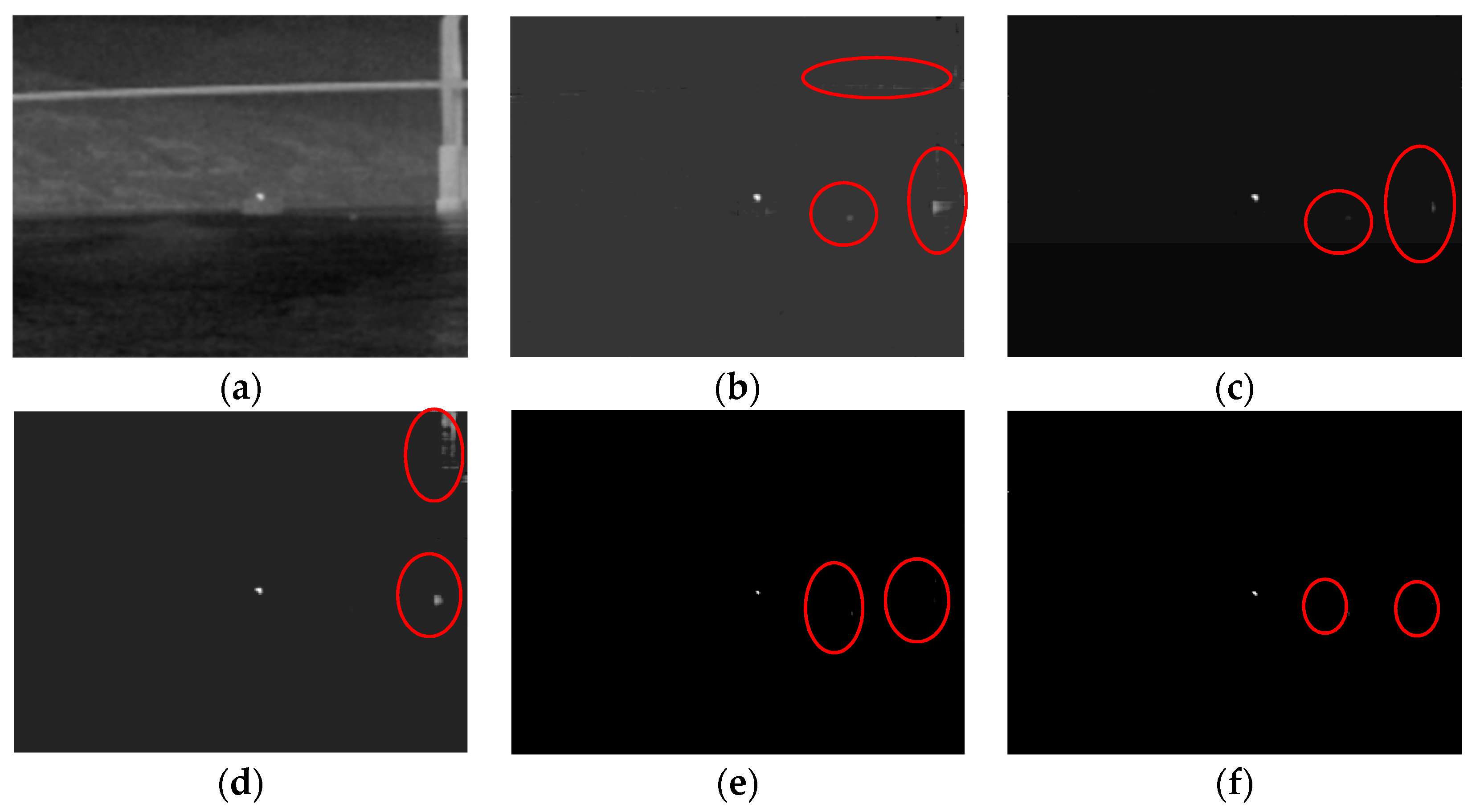
With simple homogenous scenes, most of the listed methods can achieve good results. Table 1 shows that almost all of the approaches had a poor performance when facing real complex scenes or strong edges generated by the non-target interference sources. To improve the detection ability in complex backgrounds with non-target interference sources, we proposed a novel approach based on non-convex rank approximation minimization (NRAM) and the weighted l₁ norm. Figure 1 shows the recovered target image of one typical scene via IPI, NIPPS, ReWIPI, SMSL, and RIPT, respectively. Considering the common challenge that most state-of-the-art methods currently face, which is the inability to completely sweep the strong edges and interferences as observed in Figure 1, the strong edges left in the target images are of linearly structured sparsity with respect to the whole image because of the streamlined appearance of real objects and the fact that most of the buildings contain perpendicular edges [49]. The l_2,1 norm can identify the sample outliers, most of which are related to sparse structures. Hence, to better suppress strong edges, we introduce an extra regularization term on residual strong edges utilizing the l_2,1 norm.

The main contributions of this paper are as follows:

(1).

We developed a novel infrared small target detection method based on non-convex rank approximation minimization and the weighted l₁ norm, which can approximate rank function and l₀ norm better, leading to a better ability to separate the target from the background than the state-of-the-art methods including IPI, NIPPS, ReWIPI, SMSL, and RIPT.

(2).

Considering that most of the existing approaches suffer from residual strong edges, we introduced an additional regularization term on the remaining edges utilizing the l_2,1 norm because of the linearly structured sparsity of most interference sources.

(3).

An optimization algorithm based on ADMM with DC programming was presented to solve the proposed model. Since the constraints are more powerful than the IPI-based methods, the proposed algorithm converged faster.

3. Proposed Method

On the whole, an infrared image with a small target can be regarded as

$$f_D=f_B+f_T+f_N$$

(3)

where $f_D$, $f_B$, $f_T$, $f_N$ are the original image, the background image, the target image and the noise image, respectively. As mentioned in Section 1, Gao et al. [21] presented a more general model to describe the original infrared image named IPI model based on the patch-image constructed by vectorizing the matrix within the sliding window, which is in the form of Equation (1). Since the infrared background changes slowly, this means the patches are highly correlated with both local and global patches. In other words, B is a low-rank matrix. Additionally, the small target only occupies a spot of pixels, so that T is a sparse matrix with respect to the whole image. To separate the background and target is to seek two solutions adapted to the original condition.

3.1. The Surrogate of Rank

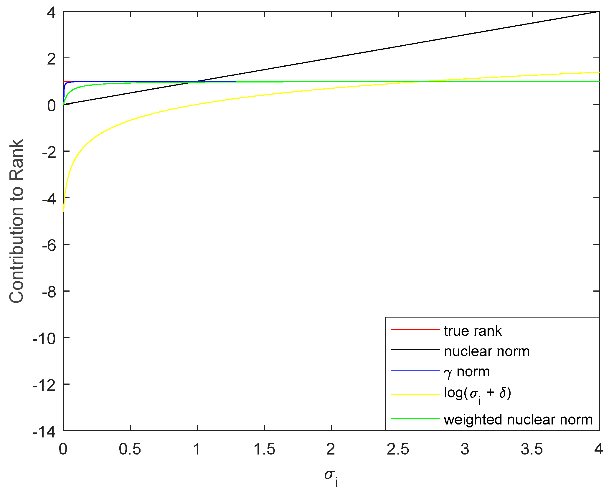
To provide a tighter approximation than the nuclear norm does, Zhao et al.[50] proposed a novel non-convex function to directly approximate the rank named as the γ norm. Note that the γ norm is actually a pseudo norm. The γ norm of matrix B is

$${\Vert B\Vert }_{\gamma }={\displaystyle \sum _i\frac{(1+\gamma ){\sigma }_i(B)}{\gamma +{\sigma }_i(B)}},\gamma >0$$

(4)

It can be observed that $\underset{\gamma \to 0}{\lim }{\Vert B\Vert }_{\gamma }=\mathrm{rank}(B)$ and $\underset{\gamma \to \infty }{\lim }{\Vert B\Vert }_{\gamma }={\Vert B\Vert }_{\ast }$. Furthermore, for any orthonormal $U\in R^{m\times m}$ and $V\in R^{n\times n}$, ${\Vert B\Vert }_{\gamma }={\Vert UB{V}^{\mathrm{T}}\Vert }_{\gamma }$, namely, the γ norm is unitarily invariant. Figure 2 indicates several surrogates of rank in the literature. Obviously, the γ norm is almost in line with the true rank (γ = 0.002 is used here), solving the imbalanced penalization by different singular values in a traditional convex nuclear norm, while the nuclear norm deviates considerably if the singular value is far away from 1 because of the equal treatment mechanism. The log-det heuristic [51] is poor at small singular values, especially those close to 0. As can be seen, the weighted nuclear norm fits the reality better than both the nuclear norm and log-det heuristic; however, every time the weight is determined, extra singular value decomposition (SVD) occurs (see more details in Reference [24]), which increases the running time of the algorithm. To maintain both accuracy and speed, the γ norm is the best candidate to describe the rank of a background patch-image.

3.2. The Surrogate of Sparsity

Given that dealing with the non-convex non-smooth l₀ norm is NP-hard, many methods [52,53,54] utilize the l₁ norm to depict the sparsity of the target patch-image. Similar to the nuclear norm, the l₁ norm gives every single element the same weight; this is a dilemma when there exist many strong edges and non-target sparse points. Taking into account that the brightness of most non-target sparse points is lower than that of small targets, a weighted l₁ norm [28] can be used to describe the target patch-image more accurately, which is given as

$${\Vert T\Vert }_{W,1}={\displaystyle \sum _{ij}{W}_{ij}}\left|T_{ij}\right|$$

(5)

$$W_{ij}=\frac{C}{\left|T_{ij}\right|+{\epsilon }_T}$$

(6)

where $W_{ij}$ is one element of the weight matrix $W$ at position $(i,j)$; C is a compromising constant and ${\epsilon }_T$ is a small positive number to avoid dividing by zero.

As analyzed in Section 2, many state-of-the-art approaches fail to address the strong edges well with complex backgrounds, leaving residuals in the target images. To deal with this problem and considering the strong edges left in the target image are of linearly structured sparsity with respect to the whole image, we introduced the l_2,1 norm to efficiently remove the residuals, which is defined as

$${\Vert E\Vert }_{2,1}={\displaystyle \sum _i\sqrt{{\displaystyle \sum _j{E}_{ij}^2}}}$$

(7)

where E denotes the sparse residual edges(w.r.t the whole patch-image).

Then, the proposed infrared patch-image model via non-convex rank approximation minimization (NRAM) is formulated as follows:

$$\begin{array}{l}\min {\Vert B\Vert }_{\gamma }+\lambda {\Vert T\Vert }_{w,1}+\beta {\Vert E\Vert }_{2,1}\\ s.t.X=B+T+E\end{array}$$

(8)

where $\lambda$ and $\beta$ are positive trade-off coefficients.

3.3. Solution of the NRAM Model

An alternating direction method of multipliers (ADMM)-based optimization algorithm was devised to solve Equation (8). By introducing a Lagrange multiplier Y and a penalty term, the constrained optimization problem becomes an unconstrained optimization problem and Equation (8) can be rewritten as the augmented Langrangian function:

$$\begin{array}{cc}\hfill L(D,B,T,E,Y,\mu )={\Vert B\Vert }_{\gamma }& +\lambda {\Vert T\Vert }_{w,1}+\beta {\Vert E\Vert }_{2,1}\hfill \\ & +\langle Y,D-B-T-E\rangle +\frac{\mu }{2}{\Vert D-B-T-E\Vert }_F^2\hfill \end{array}$$

(9)

where $\langle •\rangle$ denotes the inner product of two matrices; ${\Vert •\Vert }_F$ is the Frobenius norm. Based on ADMM, an efficient iterative approach was proposed to update $B$, $T$ and $E$, respectively. At the (k + 1)th step, update $B^{k+1}$, $T^{k+1}$ and $E^{k+1}$ by solving the following subproblems:

$$B^{k+1}=\underset{B}{\arg \min }{\Vert B\Vert }_{\gamma }+\frac{{\mu }^k}{2}{\Vert D-B-T^k-E^k-\frac{Y^k}{{\mu }^k}\Vert }_F^2$$

(10)

$$T^{k+1}=\underset{T}{\arg \min \lambda }{\Vert T\Vert }_{W,1}+\frac{{\mu }^k}{2}{\Vert D-B^{k+1}-T-E^k-\frac{Y^k}{{\mu }^k}\Vert }_F^2$$

(11)

$$E^{k+1}=\underset{E}{\arg \min }\beta {\Vert E\Vert }_{2,1}+\frac{{\mu }^k}{2}{\Vert D-B^{k+1}-T^{k+1}-E-\frac{Y^k}{{\mu }^k}\Vert }_F^2$$

(12)

Since the γ norm is a non-convex function and Equation (10) is a combination of non-convex and convex terms, it is appropriate to utilize difference of convex (DC) programming to solve Equation (10) (for details please see [50]). The DC algorithm regards the original non-convex problem as the difference of two convex functions and optimizes it iteratively by linearizing the concave term at each iteration. At the (t + 1)th inner iteration

$${\sigma }^{t+1}=\underset{\sigma \ge 0}{\arg \min }\langle {\omega }_t,\sigma \rangle +\frac{{\mu }^k}{2}{\Vert \sigma -{\sigma }_A\Vert }_2^2$$

(13)

which admits a closed-form solution

$${\sigma }^{t+1}=\max ({\sigma }_A-\frac{{\omega }_t}{{\mu }^k},0)$$

(14)

where $A=D-T^k-E^k-\frac{Y^k}{{\mu }^k}$, ${\omega }_t=\frac{(1+\gamma )\gamma }{{(\gamma +{\sigma }^t)}^2}$ and $U\mathrm{diag}\left\{{\sigma }_A\right\}{V}^{\mathrm{T}}$ is the SVD of $A$. After a few iterations (actually within two iterations), it converges to a local optimal point ${\sigma }^{\ast }$. Then, $B^{k+1}=U\mathrm{diag}\left\{{\sigma }^{\ast }\right\}{V}^{\mathrm{T}}$.

According to [55] and [28], Equations (11) and (12) can be solved as

$$T^{k+1}=S_{\lambda W/{\mu }^k}(D-B^{k+1}-E^k-\frac{Y^k}{{\mu }^k})$$

(15)

$${[E^{k+1}]}_{:,i}=\{\begin{array}{cc}\frac{{\Vert Q_{:,i}\Vert }_2-\frac{\beta }{{\mu }^k}}{{\Vert Q_{:,i}\Vert }_2}{Q}_{:,i}\hfill & \mathrm{if}{\Vert Q_{:,i}\Vert }_2>\frac{\beta }{{\mu }^k}\\ 0\hfill & \mathrm{otherwise}\end{array}$$

(16)

where $Q=D-B^{k+1}-T^{k+1}-\frac{Y^k}{{\mu }^k}$ and ${[E^{k+1}]}_{:,i}$ is the i-th column of $E^{k+1}$.

$Y$ and $\mu$ updates in the standard way:

$$Y^{k+1}=Y^k+{\mu }^k(D-B^{k+1}-T^{k+1}-E^{k+1})$$

(17)

$${\mu }^{k+1}=\rho {\mu }^k$$

(18)

where $\rho >1$. Finally, the whole process is described in Algorithms 1 and 2.

Algorithm 1: ALM/DC solver to the NRAM model

Input: Original patch-image D, λ, β, μ0, γ; Output: $B=B^k+E^k$, $T=T^k$; Initialize: $B^0=T^0=E^0=Y^0=0$, $\rho =1.1$, $\epsilon ={10}^{-7}$, $k=0$, $W^0=1\ast 1^{\mathrm{T}}$, ${\mathsf{\Lambda }}^0=0\in R^{\min (m,n)\times 1}$; While not converged do 1: Fix the others and update B by DC programming; 2: Fix the others and update T by $T^{k+1}=S_{\lambda W/{\mu }^k}(D-B^{k+1}-E^k-\frac{Y^k}{{\mu }^k})$; 3: Fix the others and update E by ${[E^{k+1}]}_{:,i}=\{\begin{array}{cc}\frac{{\Vert Q_{:,i}\Vert }_2-\frac{\beta }{{\mu }^k}}{{\Vert Q_{:,i}\Vert }_2}{Q}_{:,i}\hfill & \mathrm{if}{\Vert Q_{:,i}\Vert }_2>\frac{\beta }{{\mu }^k}\\ 0\hfill & \mathrm{otherwise}\end{array}$; 4: Fix the others and update Y by $Y^{k+1}=Y^k+{\mu }^k(D-B^{k+1}-T^{k+1}-E^{k+1})$; 5: Update W by $W_{ij}=\frac{C}{\left|T_{ij}\right|+{\epsilon }_T}$; 6: Update μ by ${\mu }^{k+1}=\rho {\mu }^k$; 7: Check the convergence conditions $\frac{{\Vert D-B^{k+1}-T^{k+1}-E^{k+1}\Vert }_F}{{\Vert D\Vert }_F}<\epsilon$; 8: Update k; $k=k+1$; End while

Algorithm 2: DC programming

Input:$B^k$, $\gamma$, $A=D-T^k-E^k-\frac{Y^k}{{\mu }^k}$, ${\mathsf{\Lambda }}^0$; Output:$B^{k+1}$, ${\mathsf{\Lambda }}^{t+1}$; Initialize:$t=0$, $[U,S,V]=\mathrm{svd}(A)$; While not converged do 1: Calculate ${\omega }_t=\frac{(1+\gamma )\gamma }{{(\gamma +{\mathsf{\Lambda }}^t)}^2}$, ${\mathsf{\Lambda }}^{t+1}=\max (S-\frac{{\omega }_t}{{\mu }^k},0)$; 2: Check the convergence conditions ${\Vert {\mathsf{\Lambda }}^{t+1}-{\mathsf{\Lambda }}^t\Vert }_2<\epsilon$; End while 3: $B^{k+1}=U{\mathsf{\Lambda }}^{t+1}V$;

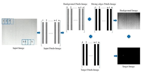
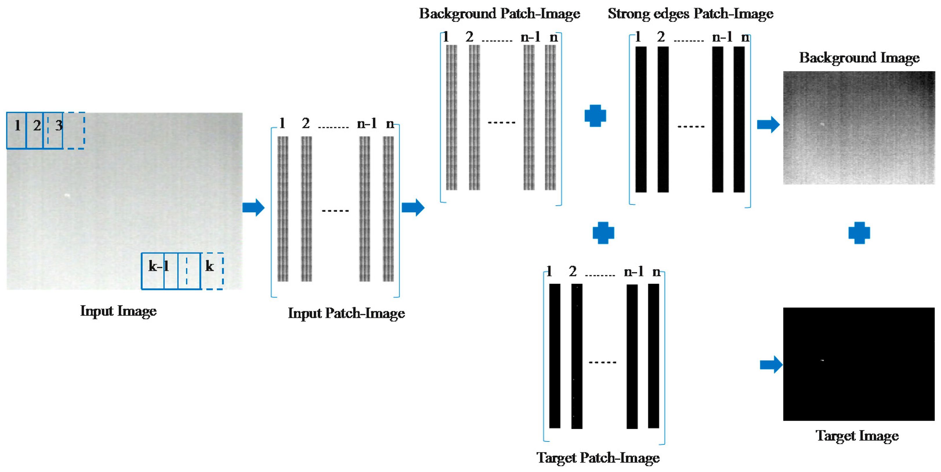
3.4. The Whole Process of the Proposed Method

Figure 3 shows the whole process of the proposed method in this paper, which can be summarized as follows:

(1).

Patch-image construction. By sliding a window of size $k\times k$ from top to bottom and from left to right to transform the original infrared image $I\in R^{m\times n}$ into a patch-image $D\in R^{k^2\times t}$, where t is the number of window slips, the matrix inside each matrix was vectorized as a column of the constructed patch-image D.

(2).

Target-background separation. The input patch-image D was decomposed into a low-rank matrix B, a sparse matrix T and a structural noise (strong edges) matrix E. Since the structural noise belongs to the background, we summed B and B as the final recovered background patch-image B.

(3).

Image reconstruction and target detection. Reconstruction is the inverse process of construction. For the position overlapped by several patches, we utilized the one-dimensional median filter to determine the value. Small targets were detected by adaptive threshold segmentation; the selection of the threshold was based on [21].

4. Experiment and Analysis

4.1. Experimental Preparation

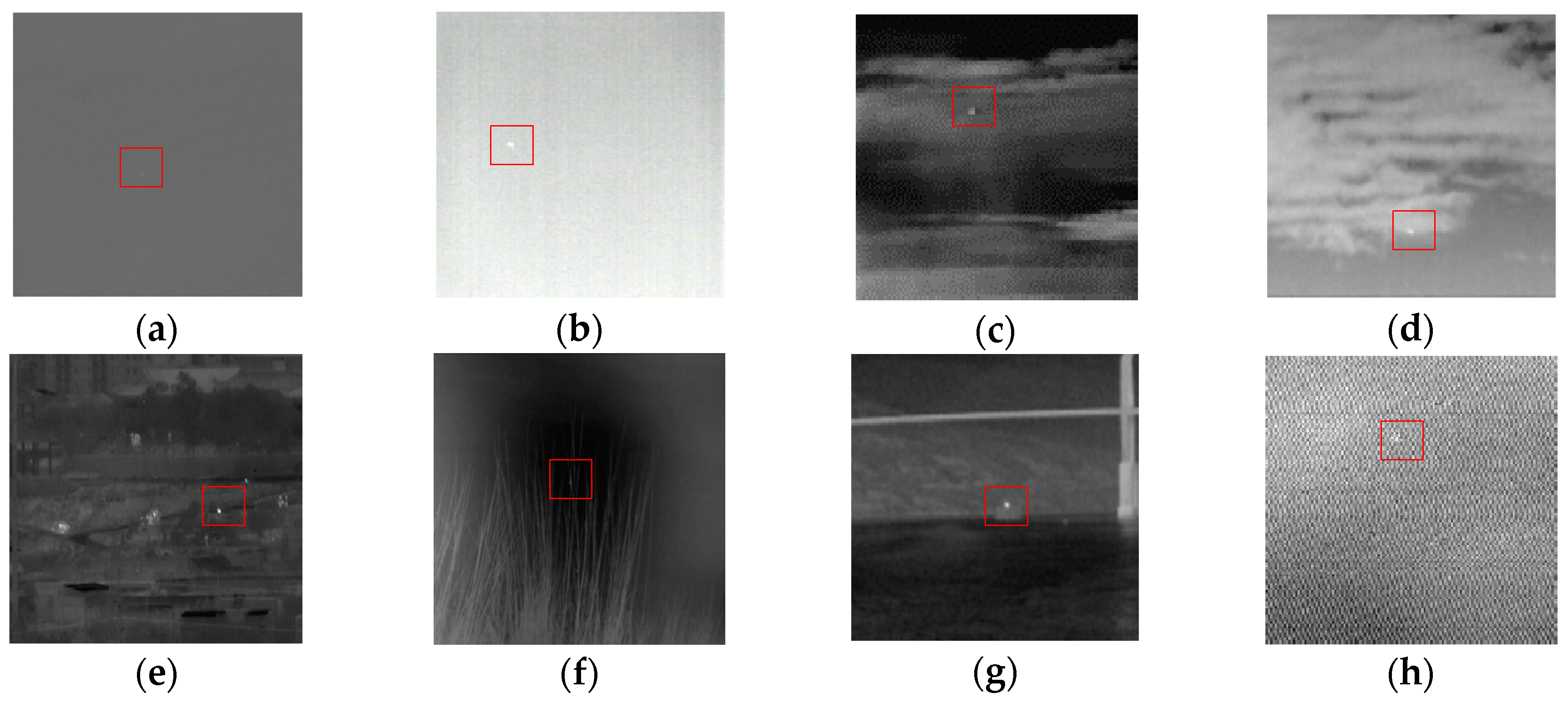
In this section, eight single practical scenes and six real sequences (the scene of each sequence was contained in the eight tested scenes) were used to test the validity of the proposed method. The eight scenes are shown in Figure 4. As most of the existing algorithms have a good effect on an infrared image with a salient target and clean background, the six sequences were not easy to deal with. Sequences 1–4 are characterized by complex backgrounds with salient strong edges and interference sources. Although both of the backgrounds were homogeneous and uniform, Sequences 5 and 6 are actually difficult because of the dim targets, which also shows the adaptability of the proposed method to different scenes. A detailed description is given in

Table 2. Detailed description of the eight real scenes.

Sequence	Frame Number	Size	Background Description	Target Description
Scene 1 (Sequence 1)	50	208 × 152	Homogenous with a highlight punctate disturbance	Small, very dim with low contrast
Scene 2 (Sequence 2)	67	320 × 240	Very bright, heavy noise	Moves fast with changing shape, brightness
Scene 3 (Sequence 3)	52	128 × 128	Sky scene with banded cloud	Tiny
Scene 4 (Sequence 4)	30	256 × 200	Heavy banded cloud and floccus	Small, size varies a lot
Scene 5 (Sequence 5)	200	252 × 220	Complex background with trees and buildings	Quite small size, changing slightly in the sequence
Scene 6 (Sequence 6)	185	252 × 213	Swinging plants that obscure the target frequently	Small, keeps moving in the sequence and changing brightness
Scene 7	—	320 × 240	Sea and mountain scene with obvious artificial structure	Ship target, bright, Gaussian shape
Scene 8	—	128 × 128	Low contrast with a lot of noise	Tiny and not so salient

. Meanwhile, eight other state-of-the-art methods including Tophat transformation [9], local contrast measure (LCM) [14], multiscale patch-based contrast measure (MPCM) [18], infrared patch-image model (IPI) [21], non-negative infrared patch-image model based on partial sum minimization of singular values (NIPPS) [43], reweighted IPI (ReWIPI) [28], stable multisubspace learning (SMSL) [47], reweighted infrared patch-tensor model (RIPT) [48] were employed as the baselines for the sake of comparison. All parameters of the seven approaches given by the authors were fine tuned for each specific sequence due to the lack of robustness of some of the approaches in addressing complex backgrounds. The final parameter settings are presented in

Table 3. Detailed parameter settings of the nine tested methods.

Method	Parameters
Tophat	Structure shape: disk, structure size: 3 × 3
LCM	Cell size: 3 × 3
MPCM	$N=3,5,7,9$, mean filter size: 3 × 3
IPI	Patch size: 50 × 50, sliding step: 10, $\lambda =1/\sqrt{\min (m,n)}$, $\epsilon ={10}^{-7}$
NIPPS	Patch size: 50 × 50, sliding step: 10, $\lambda =1/\sqrt{\min (m,n)}$ for sequence 3, $\lambda =2/\sqrt{\min (m,n)}$; for the rest, $\epsilon ={10}^{-7}$
ReWIPI	Patch size: 50 × 50, sliding step: 10, $\lambda =1/\sqrt{\min (m,n)}$ for sequence 3, $\lambda =2/\sqrt{\min (m,n)}$; for the rest, $\epsilon ={10}^{-7}$, ${\epsilon }_B={\epsilon }_T=0.08$
SMSL	Patch size: 30 × 30, sliding step: 10, $\lambda =3/\sqrt{\min (m,n)}$, ${\mu }^0=0.5\ast s_4$, $\overline{\mu }=0.05\ast s_5$, $\epsilon ={10}^{-7}$
RIPT	Patch size: 30 × 30, sliding step: 10, $\lambda =L/\sqrt{\min (m,n)}$, $L=0.7$, $h=1$, $\epsilon ={10}^{-7}$
NRAM	Patch size: 50 × 50, sliding step: 10, $\lambda =1/\sqrt{\min (m,n)}$, ${\mu }^0=3\sqrt{\min (m,n)}$, $\gamma =0.002$, $C=\sqrt{\min (m,n)}/2.5$, $\epsilon ={10}^{-7}$

. In addition, all experiments were performed with Matlab R2018a in Windows 7 based on an Intel Celeron 2.90 GHz GPU with 4 G RAM (The code is available at https://github.com/Lanneeee/NRAM).

4.2. Evaluation Metrics

For a comprehensive comparison, the whole evaluation process was based on qualitative and quantitative evaluations. All the separated target images obtained by the different methods were evaluated via several commonly used metrics to show the ability of background suppression and target enhancement, namely the signal-to-clutter ratio gain (SCRG), the background suppression factor (BSF) and the receiver operating characteristic (ROC) curve.

SCRG is the most widely used criterion whose definition is

$$\mathrm{SCRG}=\frac{\mathrm{SC}{{R}}_{\mathrm{out}}}{\mathrm{SC}{{R}}_{\mathrm{in}}}$$

(19)

where SCR is a measurement of detection difficulty and target saliency; the subscripts out and in denote the original image and the separated target image, respectively. SCR is defined as

$$\mathrm{SCR}=\frac{\left|{\mu }_t-{\mu }_b\right|}{{\sigma }_b}$$

(20)

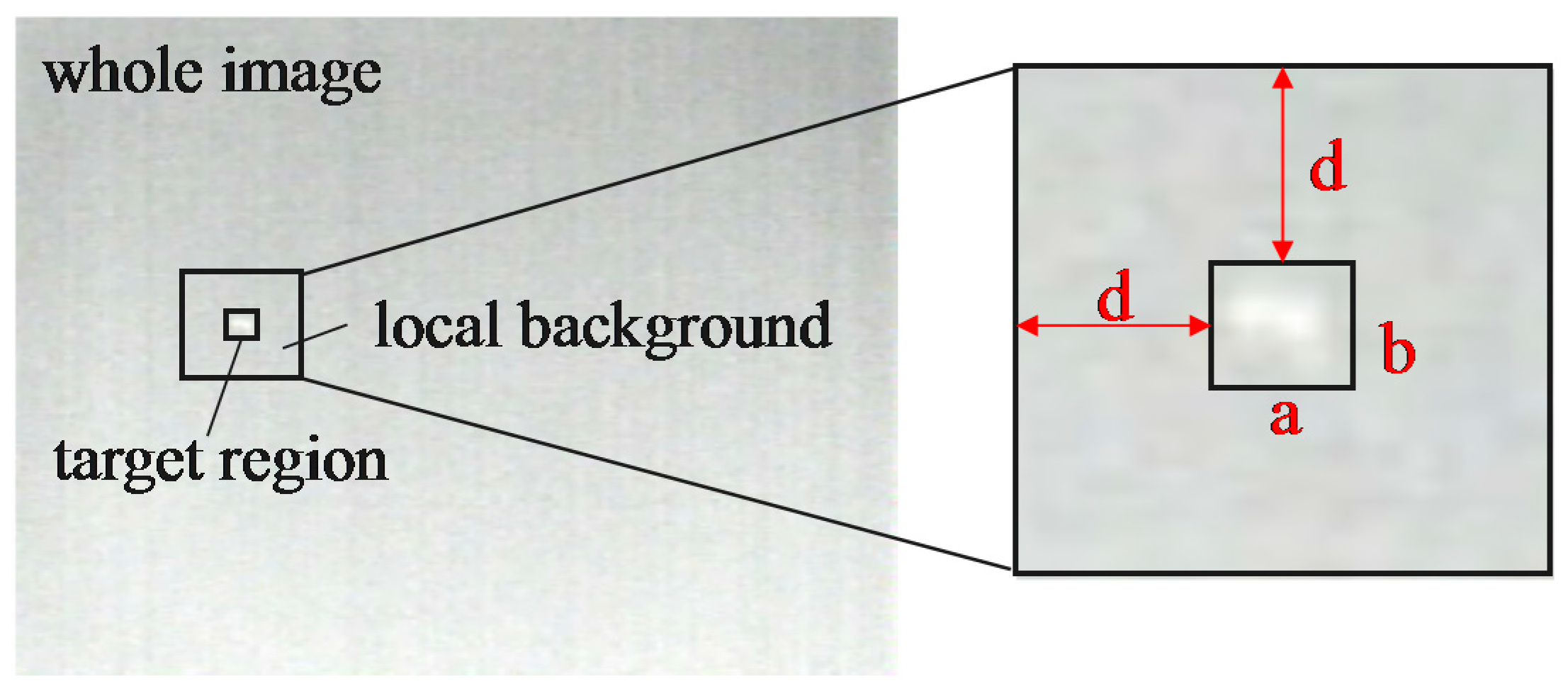
where ${\mu }_t$ and ${\mu }_b$ are the average pixel value of the target region and surrounding local neighborhood region and ${\sigma }_b$ is the standard deviation of the surrounding local neighborhood region. The local region used in the experiment is illustrated in Figure 5. The size of the target is $a\times b$, the local region size is $(a+2d)\times (b+2d)$, we set d = 40 in this paper.

Another widely used metric is BSF, showing the performance of background suppression, which is defined as

$$\mathrm{BSF}=\frac{{\sigma }_{in}}{{\sigma }_{out}}$$

(21)

where ${\sigma }_{in}$ and ${\sigma }_{out}$ represent the corresponding standard variances of the background neighborhood before and after processing. Higher SCRG and BSF values mean the better performance of an algorithm.

Besides these two metrics, the detection probability $P_d$ and false-alarm rate $F_a$ are a pair of indicators for comprehensive detection ability. $P_d$ and $F_a$ are defined as follows:

$$P_d=\frac{\mathrm{number}\mathrm{of}\mathrm{true}\mathrm{detections}}{\mathrm{number}\mathrm{of}\mathrm{actual}\mathrm{targets}}$$

(22)

$$F_a=\frac{\mathrm{number}\mathrm{of}\mathrm{false}\mathrm{detections}}{\mathrm{number}\mathrm{of}\mathrm{images}}$$

(23)

The ROC curve shows the trade-off between the true detections and false detections.

4.3. Parameter Analysis

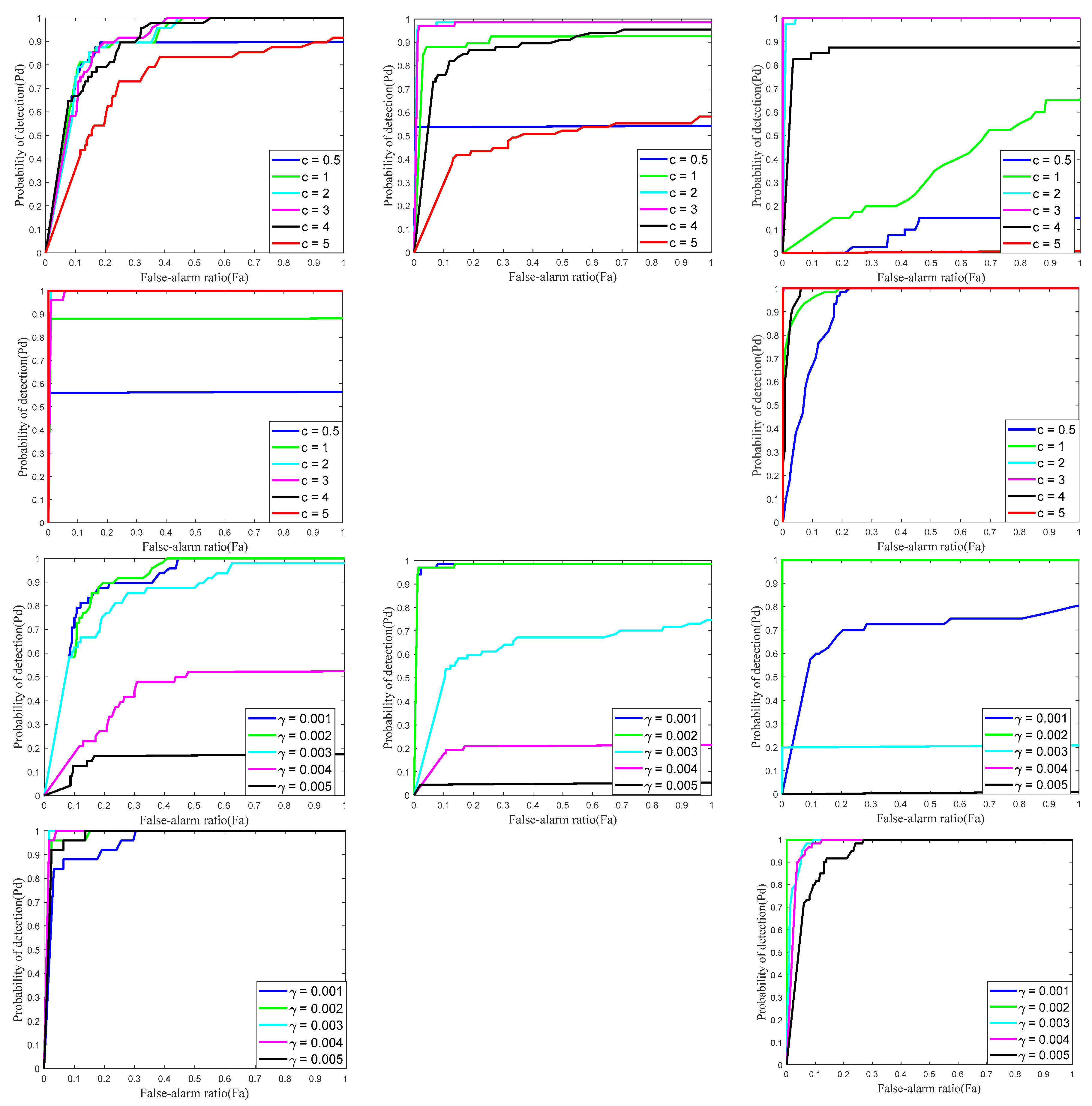
There are several vital parameters like the penalty factor $\mu$, the compromising constant C that determines the weight coefficient matrix and the norm factor $\gamma$ that affects the low-rank approximation. Hence, to obtain a better performance with real datasets, it is necessary to choose proper parameters. The ROC curves corresponding to different parameters are shown in Figure 6 for Sequences 1–5. It should be noted that the performances obtained by tuning one of the parameters with the others fixed may not be globally optimal.

4.3.1. Penalty Factor $\mu$

$\mu$ has a direct impact on the whole process, especially the soft-thresholding operator which determines the target component, thus one has to choose $\mu$ properly in order to ensure both optimality and fast convergence rate. A smaller $\mu$ would improve the ability of preserving details in the background image; however, the details of the target might also be recovered, leading to over-shrinking of the small target or no target in the target image. On the other hand, a larger $\mu$ can protect the target but would also leave more noise in the target image. In fact, the small singular value corresponds to the noise in the image, as illustrated in Figure 2; the γ norm fit the true rank well in most cases but when it came to the singular value that approached zero, the weight given to it dropped sharply until reaching zero, leading to an over-smooth background and a noisy target image. To address this problem, a larger $\mu$ is needed. Furthermore, a larger $\mu$ conducts a faster convergence. In order to change $\mu$ adaptively, we set $\mu =c\sqrt{\min (m,n)}$, where m and n are the length and width of patch image and $c$ is a positive constant. To figure out the influence of the penalty factor on Sequences 1–5, instead of changing $\mu$ directly, we varied $c$ from 0.5 to 5. For all 5 sequences, c = 2 or 3 achieved the best performance, while c = 0.5 or 5 performed the worst. This is because a smaller $\mu$ would lose the target and a too large $\mu$ would regard the salient non-target noise as the “true” target, also resulting in incorrect recovery in most cases, especially when the target was not so prominent. In fact, c = 2 shrank the target a little. We chose c = 3 as the best value.

4.3.2. Norm Factor $\gamma$

$\gamma$ is an important factor determining the ability of background recovery. With smaller $\gamma$, the rank surrogate $\gamma$ norm closely matches the true rank. However, if $\gamma$ is too small, the target would also be treated as a low-rank component. Apparently, $\gamma$ cannot be too large as that leads to deviation from the real rank, just as the nuclear-norm does. Thus, it is important to find an appropriate value for $\gamma$ to keep the balance between detection probability and the false-alarm ratio. We show the effects of $\gamma$ in the third and fourth rows of Figure 6. We varied the value of $\gamma$ from 0.001 to 0.005 with an interval of 0.001. It can be observed that even if $\gamma$ changes slightly, this change has a great impact on the results. $\gamma =0.002$ remained at a stable level while the rest had some fluctuations. The larger the $\gamma$, the worse the performance, thus the best choice for $\gamma$ was 0.002.

4.3.3. Compromising Constant C

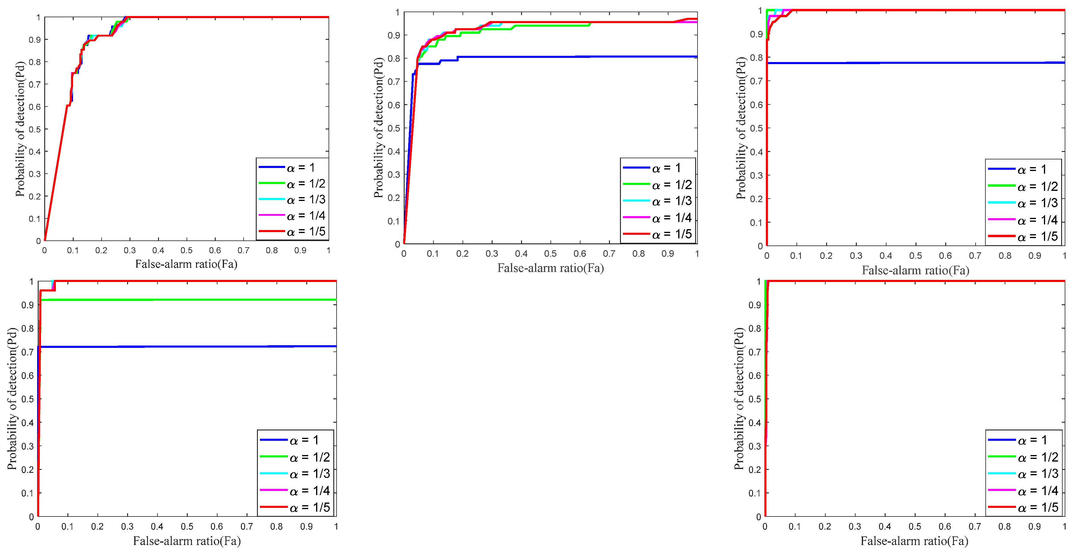
C plays an important role in controlling the adaptive weight value, which has to be chosen carefully. With reference to [24] with slight modification, we set C as $\alpha \sqrt{\min (m,n)}$ in our experiment for the sake of self-adaption. The performance of different α is shown in the last two rows of Figure 6, from which we can conclude that the algorithm was quite insensitive to the variation of C. Different C all performed well on Sequence 5 resulting from the target being easy to detect while the non-target noise was hard to suppress. Synthesizing the results of all sequences, we set $\sqrt{\min (m,n)}/2.5$ as the optimum value.

4.4. Qualitative Evaluation under Different Scenes

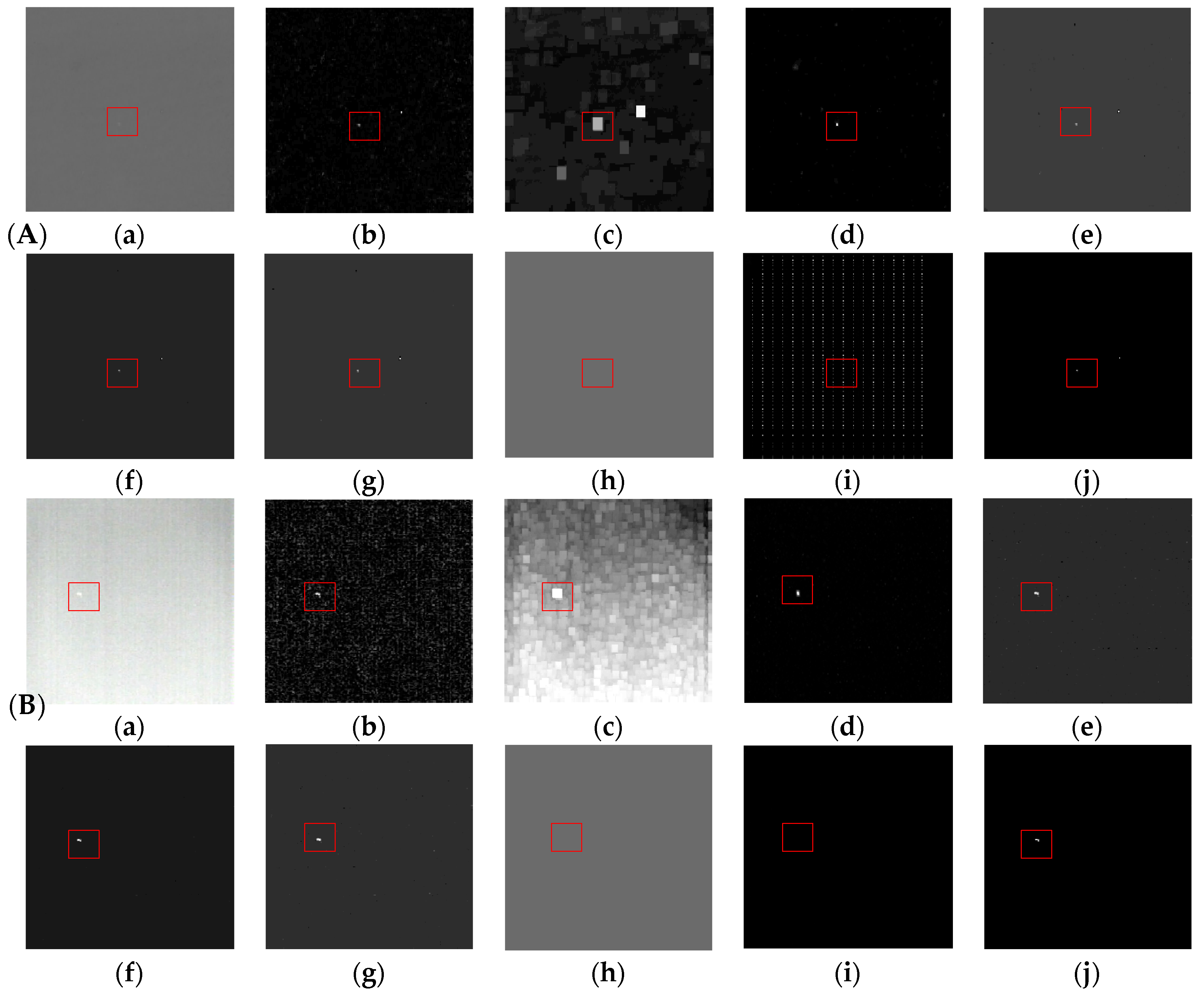
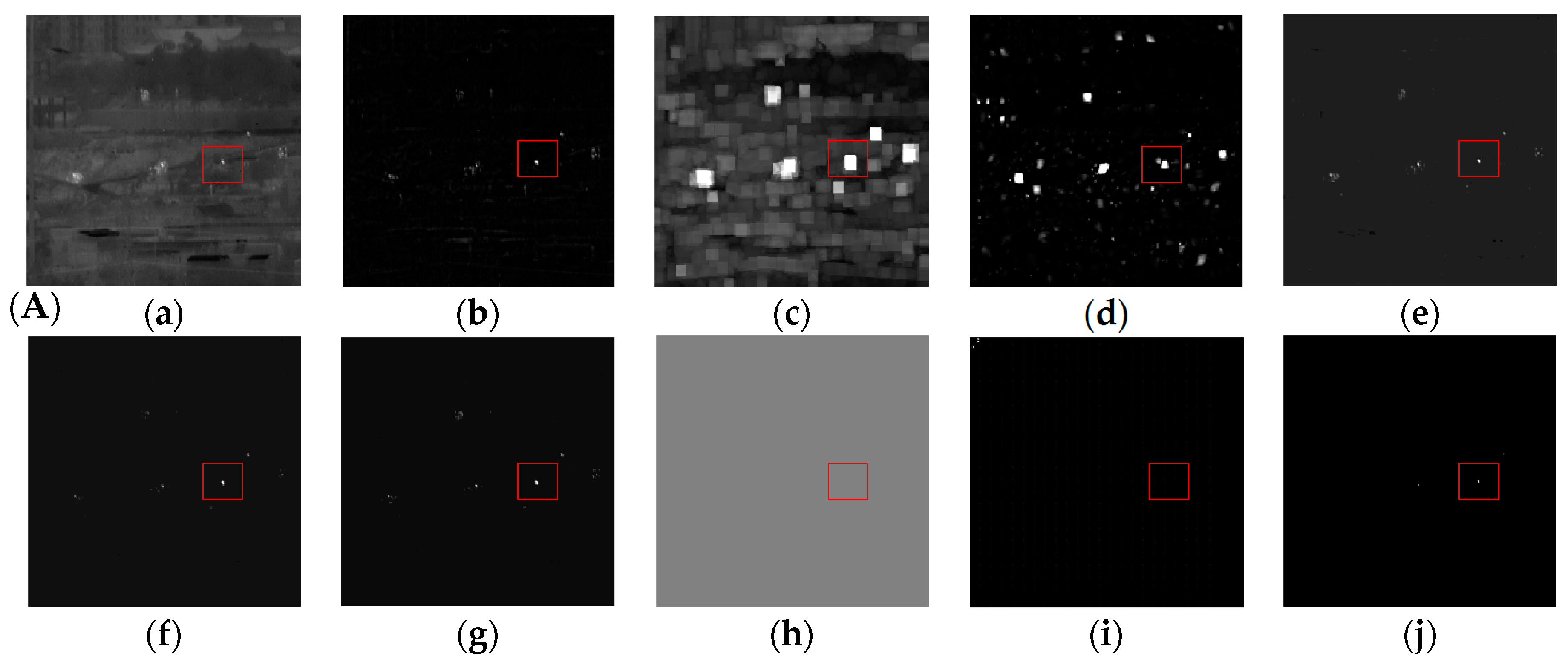
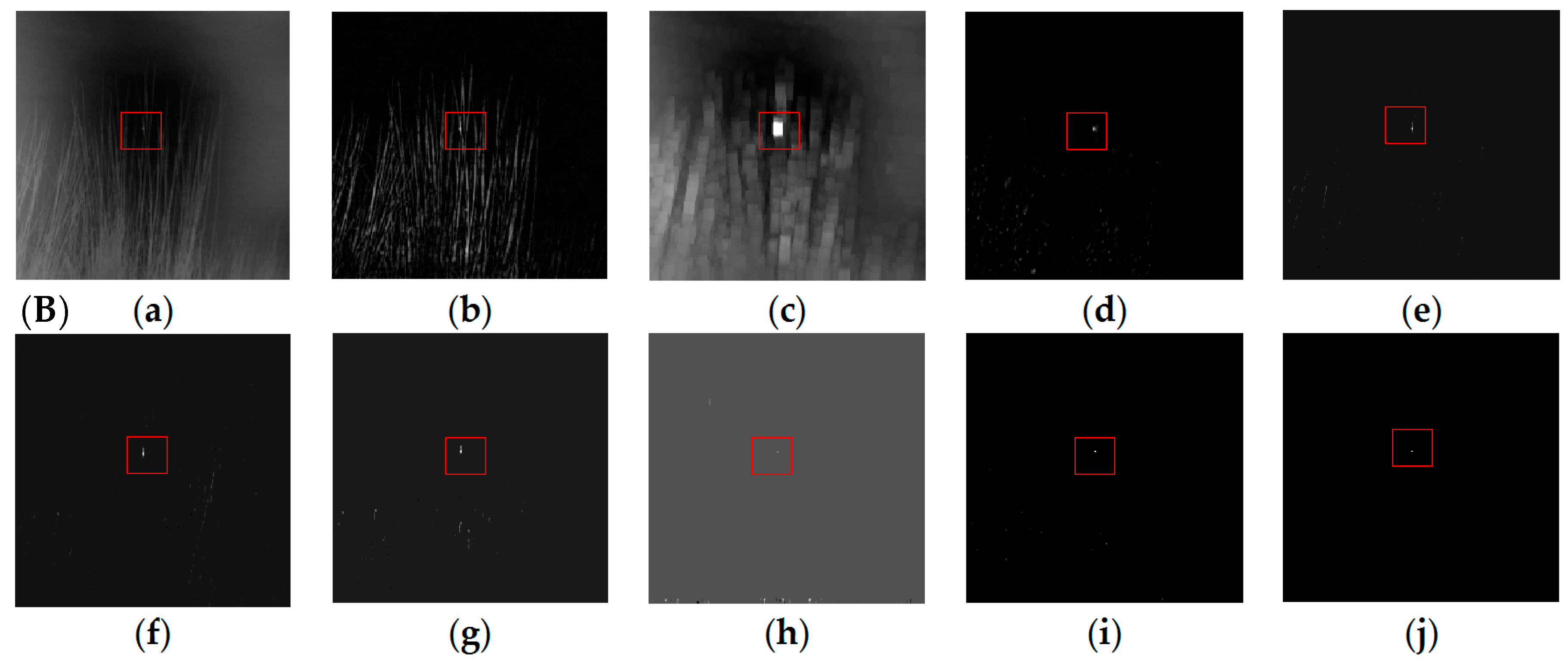
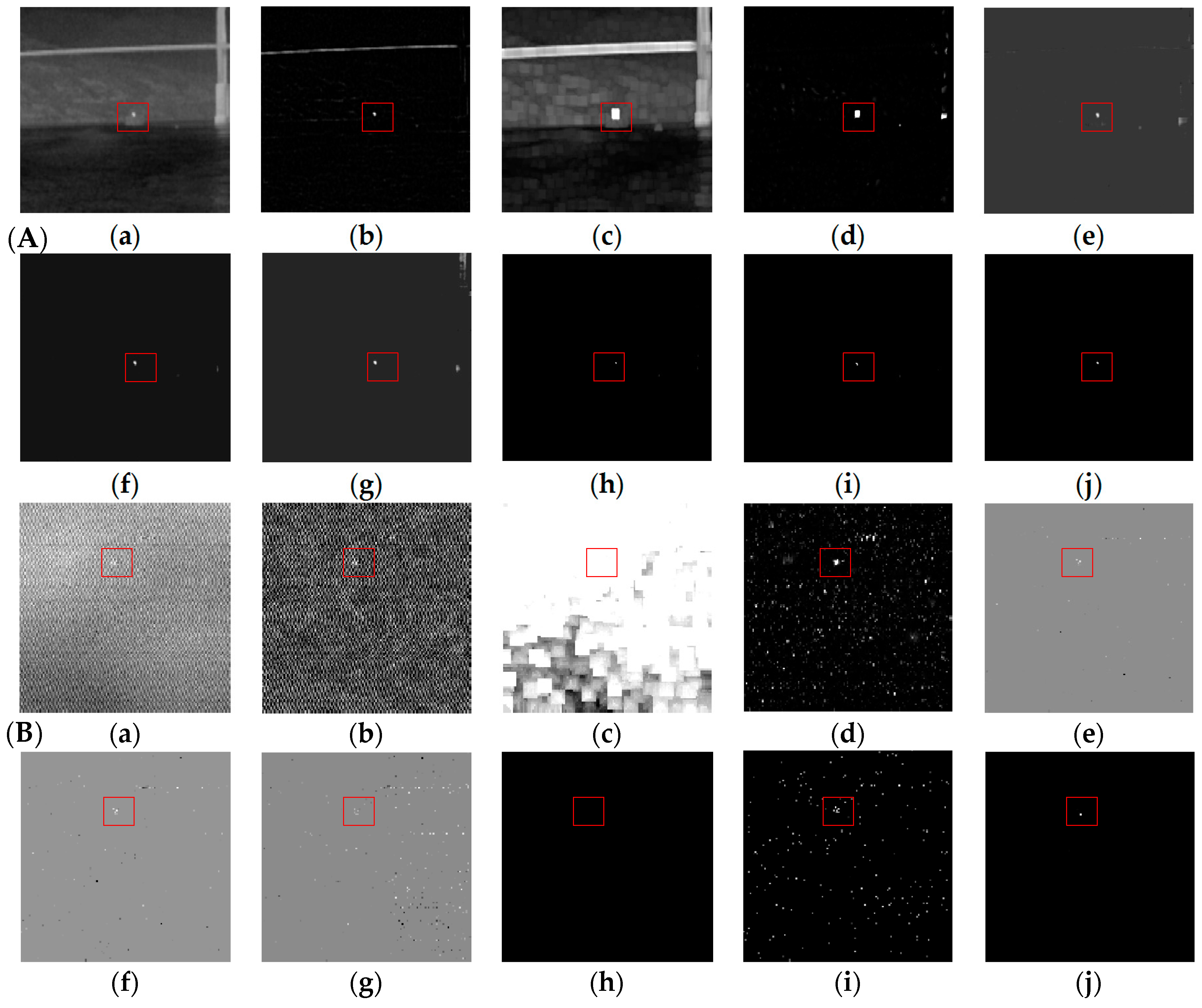
In this section, the proposed method was compared with eight state-of-the-art methods in background suppression performance. Figure 7, Figure 8 and Figure 9 are the results obtained by all the tested methods under different scenes. Note that the target has been marked with a red box.

The Tophat operator did enhance the target; however, it was extremely sensitive to edges and noise leading to a high false-alarm ratio, especially in the case of a complex background such as in Figure 8A, Figure 9B and Figure 10B. The main reason comes down to the fixed structure element and the hypothesis of smooth background. There is no doubt that the performance of the LCM was the worst among all results produced by the tested methods. This is because the contrast mechanism was not so applicable with a complex background. Moreover, when the local region of the target had low contrast, some other strong edges or brighter non-target components were highlighted instead. The worst was in Figure 10B because the contrast was almost uniform everywhere. Unlike LCM, another HSV-based approach, MPCM, defines the local contrast measure based on the difference between the reference patch and the background patches and not on the ratio of the maximum grayscale of the central cell to the average value of the surrounding cells. MPCM worked much better when facing different backgrounds, particularly in clean and uniform scenes such as in Figure 7 and showed more robustness when compared with LCM. Nevertheless, from Figure 8, Figure 9 and Figure 10, we can see that it still suffered from salient non-target objects caused by the inaccuracy of the local dissimilarity measure. In other words, the simple local dissimilarity measure or assumption based on background consistency cannot deal with various scenes.

The other five baselines aim at separating the background and target by solving optimization problems, which have relative superiority over conventional approaches. From the obtained target images, it was clear that IPI could recover the target well while also preserving the background residuals because of the deficiencies of both the nuclear norm and l₁ norm, as analyzed in Section 1. This phenomenon was most conspicuous when the target was very dim and the background edge was abundant such as in Figure 8A. NIPPS was better than IPI and could suppress most of the strong clutter and keep the shape of the target by minimizing the partial sum of singular values. Still, as observed in Figure 8, complex scenes including highlight interference sources and intensive noise is a challenge for NIPPS. By observing Figure 8, Figure 9 and Figure 10, it can be said with certainty that the NIPPS model does not satisfy scenario robustness. Furthermore, the rank estimation task was harder to address when salient clusters and non-target components exist, as shown in Figure 9A and Figure 10B. Based on the weighted nuclear norm minimization, ReWIPI applies weighted technology to restore background and target simultaneously. However, this method showed little improving effect given that, considering the backgrounds in Figure 9, the residual problem of sparse edges remained unsolved. Moreover, the convergence rate of ReWIPI was slow, resulting in high computation complexity, which will be further discussed later.

SMSL and RIPT had an unstable performance as concluded from their produced target image. From Figure 7, Figure 8A and Figure 9A, both approaches lost the target totally. For SMSL, when the target was so dim that it was difficult to distinguish the target from the background clearly, the learning mechanism would assign the target to a subspace of the background, thus the target would disappear. In addition, in Figure 8B, spot-like components lying on the boundaries would also bring about false detection because of the inaccuracy of the subspace construction. With the purpose of wiping out disturbance caused by complex backgrounds, RIPT utilizes the local structure tensor to suppress the salient background edges, which need an obvious structure. RIPT indeed achieved a good performance with some heterogeneous scenes such as in Figure 8B and Figure 10A, with the help of the structure tensor. Unfortunately, like in Figure 7, a dim target overwhelmed by background clutter did not meet the requirement and fuzzy edges even caused strange detection results. Merely using the single prior of background and not incorporating it with the target prior also explained the bad results.

Compared with all of the above baselines, it can be concluded that the proposed NRAM model provided satisfactory performances in various scenes not only in keeping the shape of the target but also in wiping out rare clutter, especially in Figure 8, Figure 9 and Figure 10 whose targets were dim and the disturbances were strong. In Figure 10B, when the target was seriously disturbed by noise, all baselines failed to detect the target and only the proposed NRAM worked relatively well even though the given target had been shrunk because of the overwhelming clutter. This demonstrates the strong scenario robustness that is lacking in the other state-of-the-art methods.

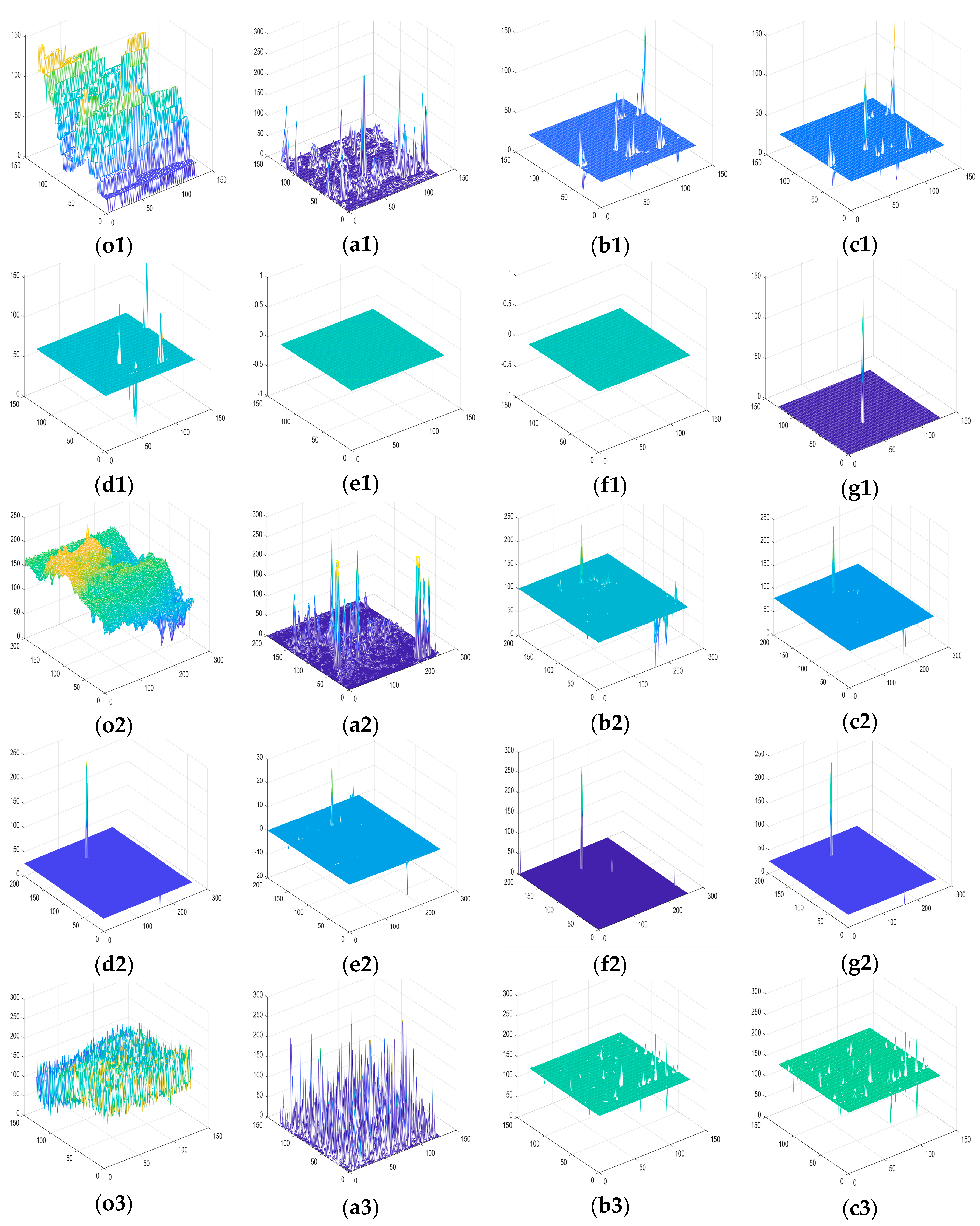
To visualize the complexity of the scenes and to compare the effectiveness of the other seven methods more intuitively, 3D gray maps of several representative tested images and obtained images (Figure 8A,B and Figure 10B) are displayed in Figure 11. It was obvious that the three scenes were all complex. From Figure 11, we can see that background components usually exist with a brightness close to or above the targets, which makes it more difficult to detect infrared dim targets accurately. MPCM enhanced the targets as well as the clutter, leaving a locating challenge. IPI, NIPPS and ReWIPI performed relatively well in most cases but there were two drawbacks: first, some strong clutter was not removed; and second, the degree of background suppression was not high (in other words, in the 3D gray maps, the minimum gray value did not reach 0). In contrast, the proposed NRAM model almost completely suppressed the background and clutter with fewer false alarms, showing strong robustness. Moreover, in the third scene, all but the proposed method were not successful. Hence, from a qualitative perspective, the NRAM model has huge advantages.

4.5. Quantitative Evaluation of Sequences

Aside from the qualitative evaluation based on different scenes, to evaluate the ability of background suppression and target enhancement in a quantitative way, evaluation indices including signal-to-clutter ratio gain (SCRG) and background suppression factor (BSF) were used to assess the performance. The experimental results of six actual sequences (Figure 7, Figure 8 and Figure 9) are shown in

Table 4. SCRG and BSF values of the nine methods.

Method	Seq 1 SCRG BSF	Seq 2 SCRG BSF	Seq 3 SCRG BSF	Seq 4 SCRG BSF	Seq 5 SCRG BSF	Seq 6 SCRG BSF
Tophat	4.92	2.09	1.54	2.29	3.78	0.53
	5.55	10.66	7.55	8.59	3.00	0.47
LCM	0.49	0.75	2.17	0.25	0.40	0.91
	0.69	0.93	1.18	0.69	0.96	0.95
MPCM	4.56	2.05	1.22	0.49	2.59	2.44
	5.49	8.20	6.85	1.96	2.50	3.76
IPI	7.36	7.64	2.59	4.24	2.10	3.25
	2.25	2.10	4.46	5.08	4.29	3.08
NIPPS	35.85	11.48	2.89	4.03	3.94	6.29
	14.32	4.42	7.30	5.61	11.84	3.95
ReWIPI	10.71	11.01	3.26	3.40	2.03	2.52
	6.72	2.93	8.36	3.18	3.93	2.58
SMSL	—	1.86	2.80	—	—	—
		10.34	2.99
RIPT	—	4.39	2.12	—	—	—
		23.39	11.5
NRAM	87.34	11.02	2.72	8.81	7.75	7.87
	60.30	50.01	21.29	25.70	32.58	59.21

NOTES: Red represents the highest value and blue represents the second highest value.

. Note that because SMSL and RIPT failed in most cases, the corresponding quantitative values were not calculated. It can be seen that the proposed method almost always achieved the highest values, showing great superiority in background suppression. In general, as before, the last six methods were better than the former simple assumption-based methods and there was no surprise that the LCM obtained the lowest scores.

To further demonstrate the advantages of the developed method, we provide the receiver operating characteristic (ROC) curves of the test sequences used in Table 4, whose horizontal axis was the false-alarm ratio of the sequence and whose vertical axis was the probability of detection of the sequence. The ROC curves are illustrated in Figure 12. Note that again, we did not consider the SMSL and RIPT for the same reason. Tophat always performed the worst since the simple structural elements could not handle the complex background. The performance of MPCM fluctuated greatly. For Sequences 1 and 2, MPCM worked very well but failed in the other sequences, which confirmed that MPCM is poor at addressing scenes filled with clutter and disturbances. IPI, NIPPS and ReWIPI achieved similar results, with the latter two performing slightly better than IPI on the whole. The biggest difference was in Sequence 3, which showed that ReWIPI performed the worst out of all methods. In general, the proposed method almost always reached the highest detection probability with respect to the same false-alarm ratio, implying that the proposed method outperformed the other state-of-the-art methods.

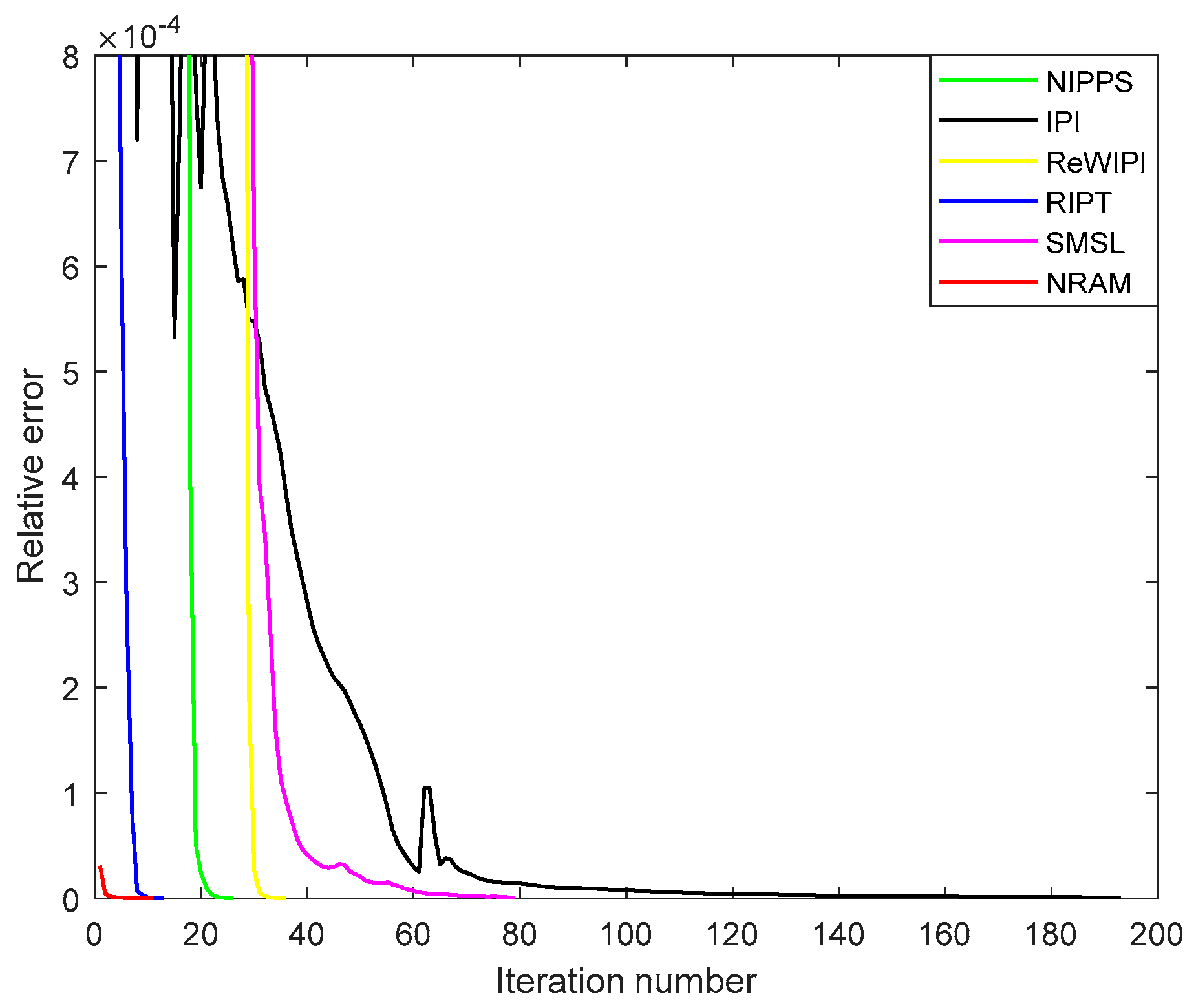
Figure 13 displays the convergence rates of the last six methods. For the sake of comparison, the maximum value of relative error was set to 0.0008. Meanwhile, the condition of stopping iteration was that the relative error was less than 10⁻⁷ for all of the used methods. The IPI model and SMSL model both had slow convergence rates resulting from time-consuming APG, while the rest were based on the faster ADMM. Compared with IPI, the number of iterations in the proposed method was about 1/20 that of the IPI model. The RIPT model converged as fast as the NRAM, however, it had trouble dealing with the very dim target.

Moreover, to compare the computational cost of the nine methods more clearly,

Table 5. Comparison of computational complexity and computing time of nine methods.

	Tophat	LCM	MPCM	IPI	NIPPS	ReWIPI	SMSL	RIPT	NRAM
Complexity	O(I2logI2MN)	O(K3MN)	O(K3MN)	O(mn2)	O(mn2)	O(kmn2)	O(lmn)	O(mn2)	O(mn2)
Time(s)	0.022	0.074	0.089	11.907	7.486	15.469	1.245	1.352	3.378

shows the algorithm complexity and computing time for Figure 8B. Suppose the image size is and m, n are the rows and columns of the patch-image. The computational cost of Tophat is O(I²logI²), where the I² is the size of the structure element. Considering the image size, the final cost of Top-Hat is O(I²logI²MN). For LCM and MPCM, it is obvious that the major time-consuming part is calculating the saliency map pixel by pixel. A sliding window of size is needed for computing the saliency value of the central pixel. Thus, k² to 8k² times mathematical operation per pixel is required, namely, in a single scale, the computational cost is O(k²MN). Therefore, the total cost in all scales is O(K³MN). For the rest of the methods, except for SMSL, the dominant factor is singular value decomposition (SVD), which has a computational complexity of O(mn²). Since an iterative reweighted scheme is used in ReWIPI, the cost of ReWIPI is O(kmn²). For SMSL, its complexity is determined by the subspace dimension and the matrix size, that is, O(lmn), where l denotes the subspace dimension.

It can be seen that the methods based on target and background separation (i.e., the last six methods) are generally slower than the filtering and HSV-based methods (i.e., the first three methods), resulting from the iterative procedure and singular value decomposition (SVD). However, considering the robustness and performance of each method, this sacrifice is acceptable. In addition, although SMSL and RIPT were faster than NRAM, their performances were not satisfactory in many cases. Therefore, there is no doubt that the developed NRAM model not only improves background suppression and target detection with complex backgrounds but also reduces the computational complexity compared with most baseline approaches.

5. Discussion

The separation of target and background utilizing optimization methods and sparse representation is widespread in the field of infrared small target detection based on the non-local self-correlation of infrared background and the sparsity of the target. The classic IPI exploits the nuclear norm to represent the low-rank patch-background matrix and when the infrared images are uniform, it works well. However, as discussed in Section 3, the larger the singular values, the farther the nuclear norm deviates. In fact, large singular values contain more details and information of the image. In other words, the nuclear norm cannot handle complex infrared scenes because of the rich details, which causes residuals and the reconstructed background is blurred. This is also the case with the l₁ norm. Unbalanced weights result in incomplete target reconstruction; that is the aforementioned over-shrink. NIPPS utilizes partial sum minimization of singular values (similar to the truncated nuclear norm) aiming to overcome the defect of the nuclear norm. One key step of NIPPS is to estimate the rank of the image, which is challenging. The small singular value of the image corresponds to the noise. Inaccurate estimation can easily minimize that part of the singular value, leading to the remaining components in the target image. ReWIPI and SMSL also make improvements to the nuclear norm and l₁ norm but still suffer from strong edges.

Currently, most state-of-the-art methods concentrate on the prior background and target, which is insufficient. RIPT introduces the structure tensor to address the problem of residuals. The performance with complex scenes is much better but unfortunately, RIPT ignores low SNR situations which lack structural information, resulting in loss of the target. Based on the IPI model, to overcome the existing problems, a tighter surrogate of rank named the γ norm with a weighted l₁ norm has been introduced to recover the background accurately. Motivated by the structural information of edges and remaining noise in the target images, the structured l_2,1 norm can handle the residuals well. Therefore, as well as the background and the target, a third component, which we called strong edges (actually not just edges), was developed. Namely, the γ norm only needs to recover a low-rank component of the background, so the weighted l₁ norm only has to reconstruct the target and the l_2,1 norm is in charge of the components that are sparse but belong to the background. A single recovery task for each component makes the problem easier to solve.

There are several vital parameters in the proposed NRAM model including the penalty factor μ, the norm factor γ and the compromising constant C. As analyzed in Section 4, the γ norm has some disadvantages but thanks to the penalty factor μ, we can overcome them. The norm factor γ, affecting how close the surrogate is to the true rank and the compromising constant C, is the key factor determining the recovery of the target image. We have discussed experiments around choosing the best value of them with self-adaption.

By comparing the performance of the proposed method with eight state-of-the-art methods from qualitative and quantitative perspectives, it is fair to say that the proposed NRAM model showed relative superiority in both background suppression and target enhancement. Furthermore, the robustness of the algorithm when faced with various scenes outperformed the baselines.

6. Conclusions

To improve the ability of background suppression with complex backgrounds, a novel method based on non-convex rank approximation minimization was proposed to reconstruct the low-rank component more accurately, namely the background. Furthermore, a more powerful sparse constraint item, the weighted l₁ norm, was exploited to enhance the target detection performance. Considering the common challenge that most state-of-the-art methods currently face, which is an inability to completely wipe out the strong edges and rare structures, an additional structured l_2,1 norm was employed to address this issue. By carefully choosing the vital parameters, an optimization algorithm combining ADMM and DC strategy was presented to solve this new model. Experimental results based on diverse scenes and sequences demonstrated that the proposed method outperformed the other state-of-the-art methods, showing more robustness and less computational complexity.

Several problems still need to be solved. For instance, if there are non-target elements at one of the four corners of the image (i.e., lower-left corner) that are much more salient than the target, all methods including the proposed NRAM model would incorrectly regard the non-target noise as the real target. Our plan is to utilize more features of targets to depict the target component better. Moreover, seeking the major dissimilarity between non-target components and targets also plays an important role. In addition, although our method reduced the computing time when compared with similar methods, it was still inferior to the traditional filtering method, which is a problem that needs to be solved.

References

- Luo, J.H.; Ji, H.B.; Liu, J. An algorithm based on spatial filter for infrared small target detection and its application to an all directional IRST system. Proc. SPIE 2007, 6279. [Google Scholar] [CrossRef]
- Tonissen, S.M.; Evans, R.J. Performance of dynamic programming techniques for Track-Before-Detect. IEEE Trans. Aerosp. Electron. Syst. 1996, 32, 1440–1451. [Google Scholar] [CrossRef]
- Reed, I.S.; Gagliardi, R.M.; Stotts, L.B.J.I.T.o.A.; Systems, E. Optical moving target detection with 3-D matched filtering. IEEE Trans. Aerosp. Electron. Syst. 1988, 24, 327–336. [Google Scholar] [CrossRef]
- Zhang, H.Y.; Bai, J.J.; Li, Z.J.; Liu, Y.; Liu, K.H. Scale invariant SURF detector and automatic clustering segmentation for infrared small targets detection. Infrared Phys. Technol. 2017, 83, 7–16. [Google Scholar] [CrossRef]
- He, Y.-J.; Li, M.; Zhang, J.; Yao, J.-P. Infrared target tracking via weighted correlation filter. Infrared Phys. Technol. 2015, 73, 103–114. [Google Scholar] [CrossRef]
- Wang, W.; Li, C.; Shi, J. A robust infrared dim target detection method based on template filtering and saliency extraction. Infrared Phys. Technol. 2015, 73, 19–28. [Google Scholar] [CrossRef]
- Zhang, H.; Zhang, L.; Yuan, D.; Chen, H. Infrared small target detection based on local intensity and gradient properties. Infrared Phys. Technol. 2018, 89, 88–96. [Google Scholar] [CrossRef]
- Wang, X.Y.; Peng, Z.M.; Zhang, P.; He, Y.M. Infrared Small Target Detection via Nonnegativity-Constrained Variational Mode Decomposition. IEEE Geosci, Remote Sens. 2017, 14, 1700–1704. [Google Scholar] [CrossRef]
- Tom, V.T.; Peli, T.; Leung, M.; Bondaryk, J.E. Morphology-based algorithm for point target detection in infrared backgrounds. In Proceedings of the Signal and Data Processing of Small Targets, Orlando, FL, USA, 22 October 1993; pp. 2–12. [Google Scholar]
- Deshpande, S.D.; Er, M.H.; Venkateswarlu, R.; Chan, P. Max-mean and max-median filters for detection of small targets. In Proceedings of the Signal and Data Processing of Small Targets, Denver, CO, USA, 4 October 1999; pp. 74–84. [Google Scholar]
- Kim, S.; Yang, Y.Y.; Lee, J.; Park, Y. Small Target Detection Utilizing Robust Methods of the Human Visual System for IRST. J. Infrared Millim. Terahertz Wave 2009, 30, 994–1011. [Google Scholar] [CrossRef]
- Shao, X.P.; Fan, H.; Lu, G.X.; Xu, J. An improved infrared dim and small target detection algorithm based on the contrast mechanism of human visual system. Infrared Phys. Technol. 2012, 55, 403–408. [Google Scholar] [CrossRef]
- Wang, X.; Lv, G.F.; Xu, L.Z. Infrared dim target detection based on visual attention. Infrared Phys. Technol. 2012, 55, 513–521. [Google Scholar] [CrossRef]
- Chen, C.L.P.; Li, H.; Wei, Y.T.; Xia, T.; Tang, Y.Y. A Local Contrast Method for Small Infrared Target Detection. IEEE Trans. Geosci. Remote Sens. 2014, 52, 574–581. [Google Scholar] [CrossRef]
- Han, J.H.; Ma, Y.; Zhou, B.; Fan, F.; Liang, K.; Fang, Y. A Robust Infrared Small Target Detection Algorithm Based on Human Visual System. IEEE Trans. Geosci. Remote Sens. 2014, 11, 2168–2172. [Google Scholar] [CrossRef]
- Qin, Y.; Li, B. Effective Infrared Small Target Detection Utilizing a Novel Local Contrast Method. IEEE Trans. Geosci. Remote Sens. 2016, 13, 1890–1894. [Google Scholar] [CrossRef]
- Han, J.H.; Liang, K.; Zhou, B.; Zhu, X.Y.; Zhao, J.; Zhao, L.L. Infrared Small Target Detection Utilizing the Multiscale Relative Local Contrast Measure. IEEE Trans. Geosci. Remote Sens. 2018, 15, 612–616. [Google Scholar] [CrossRef]
- Wei, Y.T.; You, X.G.; Li, H. Multiscale patch-based contrast measure for small infrared target detection. Pattern Recogn. 2016, 58, 216–226. [Google Scholar] [CrossRef]
- Li, J.; Duan, L.Y.; Chen, X.W.; Huang, T.J.; Tian, Y.H. Finding the Secret of Image Saliency in the Frequency Domain. IEEE Trans. Pattern Anal. 2015, 37, 2428–2440. [Google Scholar] [CrossRef] [PubMed]
- Tang, W.; Zheng, Y.B.; Lu, R.T.; Huang, X.S. A Novel Infrared Dim Small Target Detection Algorithm based on Frequency Domain Saliency. In Proceedings of the 2016 IEEE Advanced Information Management, Communicates, Electronic and Automation Control Conference (IMCEC 2016), Xi’an, China, 3–5 October 2016; pp. 1053–1057. [Google Scholar]
- Gao, C.Q.; Meng, D.Y.; Yang, Y.; Wang, Y.T.; Zhou, X.F.; Hauptmann, A.G. Infrared Patch-Image Model for Small Target Detection in a Single Image. IEEE Trans. Image Process. 2013, 22, 4996–5009. [Google Scholar] [CrossRef] [PubMed]
- Ganesh, A.; Lin, Z.C.; Wright, J.; Wu, L.Q.; Chen, M.M.; Ma, Y. Fast Algorithms for Recovering a Corrupted Low-Rank Matrix. In Proceedings of the 2009 3rd IEEE International Workshop on Computational Advances in Multi-Sensor Adaptive Processing (Camsap 2009), Aruba, Dutch Antilles, The Netherlands, 13–16 December 2009; pp. 213–216. [Google Scholar]
- Kim, H.; Choe, Y. Background Subtraction via Truncated Nuclear Norm Minimization. In Proceedings of the 2017 Asia-Pacific Signal and Information Processing Association Annual Summit and Conference (APSIPA ASC), Kuala Lumpur, Malaysia, 12–15 December 2017; pp. 447–451. [Google Scholar]
- Gu, S.H.; Zhang, L.; Zuo, W.M.; Feng, X.C. Weighted Nuclear Norm Minimization with Application to Image Denoising. In Proceedings of the 2014 IEEE Conference on Computer Vision and Pattern Recognition, Columbus, OH, USA, 23–28 June 2014; pp. 2862–2869. [Google Scholar] [CrossRef]
- Hu, Y.; Zhang, D.B.; Ye, J.P.; Li, X.L.; He, X.F. Fast and Accurate Matrix Completion via Truncated Nuclear Norm Regularization. IEEE Trans. Pattern Anal. 2013, 35, 2117–2130. [Google Scholar] [CrossRef] [PubMed]
- Sun, Q.; Xiang, S.; Ye, J. Robust principal component analysis via capped norms. In Proceedings of the 19th ACM SIGKDD International Conference on Knowledge Discovery and Data Mining, Chicago, IL, USA, 11–14 August 2013; pp. 311–319. [Google Scholar]
- Nie, F.; Huang, H.; Ding, C.H. Low-rank matrix recovery via efficient schatten p-norm minimization. In Proceedings of the Twenty-Sixth AAAI Conference on Artificial Intelligence, Toronto, ON, Canada, 22–26 July 2012; pp. 655–661. [Google Scholar]
- Guo, J.; Wu, Y.Q.; Dai, Y.M. Small target detection based on reweighted infrared patch-image model. IET Image Process. 2018, 12, 70–79. [Google Scholar] [CrossRef]
- Zhang, T. Analysis of Multi-stage Convex Relaxation for Sparse Regularization. J. Mach. Learn. Res. 2010, 11, 1081–1107. [Google Scholar]
- He, Y.J.; Li, M.; Zhang, J.L.; An, Q. Small infrared target detection based on low-rank and sparse representation. Infrared Phys. Technol. 2015, 68, 98–109. [Google Scholar] [CrossRef]
- Boyd, S.; Parikh, N.; Chu, E.; Peleato, B.; Eckstein, J.J.F.; Learning, T.i.M. Distributed optimization and statistical learning via the alternating direction method of multipliers. Found. Trends Mach. Learn. 2011, 3, 1–122. [Google Scholar] [CrossRef]
- Lin, Z.; Chen, M.; Ma, Y. The Augmented Lagrange Multiplier Method for Exact Recovery of Corrupted Low-Rank Matrices. ArXiv 2010, arXiv:1009.5055. [Google Scholar]
- Gu, S.H.; Xie, Q.; Meng, D.Y.; Zuo, W.M.; Feng, X.C.; Zhang, L. Weighted Nuclear Norm Minimization and Its Applications to Low Level Vision. Int. J. Comput. Vis. 2017, 121, 183–208. [Google Scholar] [CrossRef]
- Xue, S.; Qiu, W.; Liu, F.; Jin, X. Low-Rank Tensor Completion by Truncated Nuclear Norm Regularization. ArXiv 2017, arXiv:1712.00704. [Google Scholar]
- Cao, W.F.; Wang, Y.; Sun, J.; Meng, D.Y.; Yang, C.; Cichocki, A.; Xu, Z.B. Total Variation Regularized Tensor RPCA for Background Subtraction From Compressive Measurements. IEEE Trans. Image Process. 2016, 25, 4075–4090. [Google Scholar] [CrossRef] [PubMed]
- Tao, P.D.; An, L.T.H.J.A.M.V. Convex analysis approach to dc programming: Theory, algorithms and applications. Acta Math. Vietnam. 1997, 22, 289–355. [Google Scholar]
- Hadhoud, M.M.; Thomas, D.W.J.I.T.o.C.; Systems. The two-dimensional adaptive LMS (TDLMS) algorithm. IEEE Trans. Circuits Syst. 1988, 35, 485–494. [Google Scholar] [CrossRef]
- Zhao, Y.; Pan, H.; Du, C.; Peng, Y.; Zheng, Y. Bilateral two-dimensional least mean square filter for infrared small target detection. Infrared Phys. Technol. 2014, 65, 17–23. [Google Scholar] [CrossRef]
- Bae, T.W.; Zhang, F.; Kweon, I.S. Edge directional 2D LMS filter for infrared small target detection (vol 55, pg 137, 2012). Infrared Phys. Technol. 2012, 55, 220. [Google Scholar] [CrossRef]
- Bae, T.W.; Kim, Y.C.; Ahn, S.H.; Sohng, K.I. A novel Two-Dimensional LMS (TDLMS) using sub-sampling mask and step-size index for small target detection. IEICE Electron. Express 2010, 7, 112–117. [Google Scholar] [CrossRef] [Green Version]
- Li, Z.J.; Zhang, H.Y.; Bai, J.J.; Zhou, Z.J.; Zheng, H.H. A Speeded-up Saliency Region-based Contrast Detection Method for Small Targets. SPIE Proc. 2018, 10615. [Google Scholar] [CrossRef]
- Dai, Y.M.; Wu, Y.Q.; Song, Y. Infrared small target and background separation via column-wise weighted robust principal component analysis. Infrared Phys. Technol. 2016, 77, 421–430. [Google Scholar] [CrossRef]
- Dai, Y.M.; Wu, Y.Q.; Song, Y.; Guo, J. Non-negative infrared patch-image model: Robust target-background separation via partial sum minimization of singular values. Infrared Phys. Technol. 2017, 81, 182–194. [Google Scholar] [CrossRef]
- Oh, T.H.; Kim, H.; Tai, Y.W.; Bazin, J.C.; Kweon, I.S. Partial Sum Minimization of Singular Values in RPCA for Low-Level Vision. In Proceedings of the 2013 IEEE International Conference on Computer Vision, Sydney, Australia, 1–8 December 2013; pp. 145–152. [Google Scholar] [CrossRef]
- Li, M.; He, Y.-J.; Zhang, J. Small Infrared Target Detection Based on Low-Rank Representation. In Proceedings of the International Conference on Image and Graphics, Tianjin, China, 13–16 August 2015; pp. 393–401. [Google Scholar] [CrossRef]
- Liu, D.; Li, Z.; Liu, B.; Chen, W.; Liu, T.; Cao, L. Infrared small target detection in heavy sky scene clutter based on sparse representation. Infrared Phys. Technol. 2017, 85, 13–31. [Google Scholar] [CrossRef]
- Wang, X.Y.; Peng, Z.M.; Kong, D.H.; He, Y.M. Infrared Dim and Small Target Detection Based on Stable Multisubspace Learning in Heterogeneous Scene. IEEE Trans. Geosci. Remote Sens. 2017, 55, 5481–5493. [Google Scholar] [CrossRef]
- Dai, Y.M.; Wu, Y.Q. Reweighted Infrared Patch-Tensor Model With Both Nonlocal and Local Priors for Single-Frame Small Target Detection. IEEE J. Sel. Top. Appl. Earth Obs. Remote Sens. 2017, 10, 3752–3767. [Google Scholar] [CrossRef] [Green Version]
- Benedek, C.; Descombes, X.; Zerubia, J. Building Development Monitoring in Multitemporal Remotely Sensed Image Pairs with Stochastic Birth-Death Dynamics. IEEE Trans. Pattern Anal. 2012, 34, 33–50. [Google Scholar] [CrossRef] [PubMed] [Green Version]
- Kang, Z.; Peng, C.; Cheng, Q. Robust PCA via Nonconvex Rank Approximation. IEEE Data Min. 2015, 211–220. [Google Scholar] [CrossRef]
- Fazel, M.; Hindi, H.; Boyd, S.P. Log-det heuristic for matrix rank minimization with applications to Hankel and Euclidean distance matrices. In Proceedings of the 2003 American Control Conference, Denver, CO, USA, 4–6 June 2003; pp. 2156–2162. [Google Scholar]
- Wright, J.; Ganesh, A.; Rao, S.; Peng, Y.; Ma, Y. Robust principal component analysis: Exact recovery of corrupted low-rank matrices via convex optimization. In Proceedings of the Advances in Neural Information Processing Systems, Vancouver, BC, Canada, 7–10 December 2009; pp. 2080–2088. [Google Scholar]
- Peng, Y.; Suo, J.; Dai, Q.; Xu, W. Reweighted low-rank matrix recovery and its application in image restoration. IEEE Trans. Cybern. 2014, 44, 2418–2430. [Google Scholar] [CrossRef] [PubMed]
- Liu, Z.S.; Li, J.C.; Li, G.; Bai, J.C.; Liu, X.N. A New Model for Sparse and Low-Rank Matrix Decomposition. J. Appl. Anal. Comput. 2017, 7, 600–616. [Google Scholar] [CrossRef]
- Yuan, M.; Lin, Y. Model selection and estimation in regression with grouped variables. J. R. Stat. Soc. Stat. Methodol. Ser. B 2006, 68, 49–67. [Google Scholar] [CrossRef] [Green Version]
Figure 1.
The target image recovered by five state-of-the-art methods under one typical scene. The red circle represents the near-linear background residuals left behind. (a) Original image; (b) IPI; (c) NIPPS; (d) ReWIPI; (e) SMSL; (f) RIPT.
Figure 2.
The contribution of different surrogates to the rank with respect to a varying singular value. The true rank is 1 for a nonzero σi.
Figure 3.
The overall procedure of the roposed model in this paper.
Figure 4.
The eight real scenes used in the experiments. For the sake of visualization, all the images are changed to the same size. (a) Scene 1 (Sequence 1); (b) Scene 2 (Sequence 2); (c) Scene 3 (Sequence 3); (d) Scene 4 (Sequence 4); (e) Scene 5 (Sequence 5); (f) Scene 6 (Sequence 6); (g) Scene 7; (h) Scene 8.
Figure 5.
Local region of a small target in an infrared image.
Figure 6.
Detection performances under different parameters. Rows 1–2: ROC curves with respect to different penalty factors, Rows 3–4: ROC curves with respect to different norm factors, Rows 4–5: ROC curves with respect to different compromising constants.
Figure 7.
Results of the different approaches to Scenes 1 and 2. (A) Scene 1 (Sequence 1); (B) Scene 2 (Sequence 2); (a) Original image; (b) Tophat; (c) LCM; (d) MPCM; (e) IPI; (f) NIPPS; (g) ReWIPI; (h) SMSL; (i) RIPT; (j) NRAM.
Figure 8.
Results of different approaches to Scenes 3 and 4. (A) Scene 3 (Sequence 3); (B) Scene 4 (Sequence 4); (a) Original image; (b) Tophat; (c) LCM; (d) MPCM; (e) IPI; (f) NIPPS; (g) ReWIPI; (h) SMSL; (i) RIPT; (j) NRAM.
Figure 9.
Results of different approaches to Scene 5 and 6. (A) Scene 5 (Sequence 5); (B) Scene 6 (Sequence 6); (a) Original image; (b) Tophat; (c) LCM; (d) MPCM; (e) IPI; (f) NIPPS; (g) ReWIPI; (h) SMSL; (i) RIPT; (j) NRAM.
Figure 10.
Results of different approaches to Scenes 7 and 8. (A) Scene 7; (B) Scene 8; (a) Original image; (b) Tophat; (c) LCM; (d) MPCM; (e) IPI; (f) NIPPS; (g) ReWIPI; (h) SMSL; (i) RIPT; (j) NRAM.
Figure 11.
3D gray maps of three representative scenes and corresponding results. (a) Original image; (b) MPCM; (c) IPI; (d) NIPPS; (e) SMSL; (f) RIPT; (g) NRAM.
Figure 12.
ROC curves of detection results of six real sequences. (a) Sequence 1; (b) Sequence 2; (c) Sequence 3; (d) Sequence 4; (e) Sequence 5; (f) Sequence 6.
Figure 13.
Convergence rates of the IPI, NIPPS, ReWIPI, SMSL, RIPT and NRAM models.