A Fast Algorithm for Rail Extraction Using Mobile Laser Scanning Data


1
GNSS Research Center, Wuhan University, Wuhan 430079, China
2
School of Geodesy and Geomatics, Wuhan University, 129 Luoyu Road, Wuhan 430079, China
*
Author to whom correspondence should be addressed.
Remote Sens. 2018, 10(12), 1998; https://0-doi-org.brum.beds.ac.uk/10.3390/rs10121998
Submission received: 8 November 2018
/
Revised: 8 December 2018
/
Accepted: 8 December 2018
/
Published: 10 December 2018
(This article belongs to the Special Issue Inland Transport Networks Monitoring from Remote Sensing and Photogrammetry)
Abstract
:Railroads companies conduct regular inspections of their tracks to maintain and update the geographic data for railway management. Traditional railroad inspection methods, such as onsite inspections and semi-automated analysis of imagery and video data, are time consuming and ineffective. This study presents an automated effective method to detect tracks on the basis of their physical shape, geometrical properties, and reflection intensity feature. This study aims to investigate the feasibility of fast extraction of railroad using onboard Velodyne puck data collected by mobile laser scanning (MLS) system. Results show that the proposed method can be executed rapidly on an i5 computer with at least 10 Hz. The MLS system used in this study comprises a Velodyne puck/onboard GNSS receiver/inertial measurement unit. The range accuracy of Velodyne puck equipment is 2 cm, which fulfills the need of precise mapping. Notably, positioning STD is lower than 4 cm in most areas. Experiments are also undertaken to evaluate the timing of the proposed method. Experimental results indicate that the proposed method can extract 3D tracks in real-time and correctly recognize pairs of tracks. Accuracy, precision, and sensitivity of total test area are 99.68%, 97.55%, and 66.55%, respectively. Results suggest that in a multi-track area, close collaboration between MLS platforms mounted on several trains is required.
1. Introduction
Rail transport remains one of the most cost-effective and safe types of transportation compared to other types. Nowadays, it is still the first choice for citizens to travel in some areas [1]. Railroads conduct regular inspections of their track to meet the needs of safe transportation. Inspections of railway facilities, such as railroad tracks, contact wires, and other railway infrastructure, are vital. In this situation, existing geospatial database about railway infrastructure must be continuously updated. Among these data, the spatial data information of railroad tracks is important to railway shift arrangements, passenger comfort, and railway safety. Traditional railroad inspection methods, such as onsite inspections and semi-automated analysis of image and video data, are time consuming and ineffective. These methods can provide rich and accurate spatial information but require excellent lighting conditions (e.g., daylight and weather).
Recent years have seen the emergence of mobile laser scanning technology (MLS) [2]. Integrated with navigation sensors (e.g., Global Navigation Satellite systems (GNSS), Inertial Measure Unit (IMU)) and image acquisition sensors, MLS has remarkable performance in detection, extraction, and modeling of urban objects. MLS provides several benefits over conventional sources of data acquisition procedure in terms of accuracies, attributes, resolutions. Mapping with airborne laser scanning (ALS), terrestrial laser scanning (TLS), and MLS is common in recent years because laser scanners provide massive high-quality range measurements with intensity features in a fast manner. Many remarkable practices are made in MLS, ALS, and TLS. The ALS technology has been commercialized in the generation of high-precision digital elevation and surface models [3]. The first MMS [4] used onboard satellite receivers and stereo cameras to capture road images. At that time, precise point positioning [5] technology and differential positioning [6] technology were not introduced yet. IMUs are expensive and the application of mobile mapping systems (MMSs) is limited. Currently, Crucial high-end MMSs such as the Optech Lynx mobile mapping system, Trimble MX-9 MLS system, and RIGEL VMX-2HA MLS system could capture over millions of points every second. Commercial MMSs are applied to point cloud data acquisition of urban road networks and railroad corridors. However, commercial MMSs do not provide a user programming interface, which makes object detection and extraction applications based on them impossible. Consequently, previous studies were focused on the combined use of those devices [7].
In general terms, an MLS platform is a vehicle-mounted MMS that is integrated with multiple sensors (e.g., GNSS antenna, IMU, digital cameras) and equipped with a centralized computing system for data synchronization and management. Existing urban reconstruction algorithms using data from different source (e.g., ALS, TLS, MLS) obtain convincing results in urban object modeling and management. Data collected by vehicle-mounted MMSs can be used to detect on-road objects [8] and off-road objects. The on-road points occupy the biggest part of MLS points in road. Extraction methods [2,9,10,11,12,13,14] aimed at detecting and extracting on-road objects (e.g., driving lines, road boundaries, road cracks and road manholes) performed well both in accuracy and precision. The off-road points could be used to identify and extract traffic signs, trees, power lines and light poles, holes, and cracks in sidewalks. The fusion of multi-source data [15], including RGB cameras, LiDAR, GNSS, and IMU, is the current trend of high-precision point cloud research. In the field of object recognition, point cloud data for pedestrian detection have different attributes, colors, and depths [16]. The mapping accuracy of MMSs is constantly increasing and can be used to monitor the deformation of the tunnel profile [17]. Mobile mapping technology has been widely used in urban road traffic. Moreover, MMSs have been applied in railway mapping, mainly in the survey of railroad infrastructures and railroad tracks [18,19].
Although the ideas of processing point cloud data collected for road and railroad share similarities in certain aspects (e.g., railroad tracks and road edges). In this study, algorithms applied in a railroad environment will be discussed in detail. The first data consider the situation in railroad inspection field using imagery and video. High-speed cameras and artificial light are used to capture images. Computer vision [20] and machine learning techniques [21] are conducted for post-processing analysis, rail sections are detected, and possible distortions are reported to provide a basis for railway decision making. Subsequently, aerial and airborne imagery data [22,23] are used to extract railway road lines for obtaining convincing results. Automated rail extraction methods have been subsequently proposed and well validated. Typically, a sliding window method [24] that considers the railway geometry, proximity, and intensity has been proposed and achieves automatic rail extraction in complex multi-track situations. In addition, railroad infrastructures like tracks, wires, masses, towers, signs, bridges are of vital importance to railroad management and requires monitoring for safe transportation. Automated methods [25,26,27,28,29,30] to recognize railroad infrastructure such as overhead catenary systems from 3D LIDAR data, are later developed.
In terms of the real-time processing of MLS data, Simultaneous Localization and Mapping technology has developed rapidly in recent years. Considerable research has been made to extract features from raw point cloud to realize efficient and accurate scan matching. The V-LOAM [31] method, which extracts plain and sharp points as matching features, is tested in the KITTI Vision Benchmark Suite and performs well.
This study aims to use the point cloud collected by an MMS mounted on a railcar to perform the rapid extraction of rails. With a Velodyne puck, the single frame processing time is less than the single frame scanning time. The collected point cloud data are projected to the local navigation coordinate system using spatial information and transform angles generated by the GNSS/IMU data fusion. Then, the proposed single scan line height algorithm ranks the difference and uses the sliding window method to find the local maximum value. To this end, the rail points are extracted in consideration of the geometric characteristics of the rail and the intensity characteristics of the steel structure. The isolated point is filtered to obtain a three-dimensional point cloud of the rail.
In this study, the simulation environment is built using the robot operating system (ROS). The real-time playback of the collected data is used to simulate the real test scene, and the reliability of the proposed method is verified. The rapid extraction of rails indicates that traditional human-intensive inspections are improved, and the extracted rails can be imported into 3D processing software, such as AutoCAD, for quick modeling. The main contributions of this study are:
- This study presents an automated effective method to detect tracks on the basis of their physical shape, geometrical properties, and reflection intensity features. Results show that the proposed method can be executed rapidly on an i5 computer with at least 10 Hz.
- This study proposed a detailed workflow for rail extraction. It has been tested at no GNSS signal environment. Results suggest that for a multi-track area (e.g., 8 pairs and 16 pairs of tracks), close collaboration between MLS platforms mounted on several trains is required.
The rest of the paper is structured as follows. Section 2 briefly summarizes existing methods on rail extraction. Section 3 provides a detailed workflow. This section contains the algorithm structure description in detail, data preprocessing (Section 3.1), track point extraction (Section 3.2), and detected point verification (Section 3.3). Section 4 describes the test environment and data. Section 5 presents the results and discussion. Section 6 elaborates the conclusions.
2. Related Work
Due to huge data volumes, complex and incomplete rail structures, and occlusion of features caused by moving trains and incidence angles, automated algorithms for efficient extraction or condition monitoring of railroads and railroad infrastructure lag behind, compared with the advances in MLS systems.
In some previous research, data processing procedure was carried out manually by using commercial software. Lesler et al. [19] discussed employing an MLS system in the survey of railroad corridors. Soni et al. [32] used a TLS system to scan tracks and fit 3D CAD models to perform rail extraction using software. The processing of both requires a lot of tedious, manual work.
To automate the data processing, many researchers focused on traditional and learning based methods. Relevant works on the recognition of railroad infrastructure could be classified into three categories: data-driven and model-driven methods [25] using point features and geometry relationship [33]; learning based methods [2]; and multi-source data fusion methods [22,23,34].
The data-driven and model-driven methods of automatic extraction of rails from the point cloud data of the MMS without other sources can be classified into two categories, one uses local features and the other uses global statistical characteristics [2,25,27]. Yang et al. [24,33] used the high-difference fluctuations on the local scanning line considering the low-reflection characteristics of the steel structure. The sliding window method is used to extract the rail bed first and then the rail in accordance with the relative geometric relationship between the rail and the rail bed. The method of height difference variation often extracts other class points with similar characteristics that need to be further verified. For example, filtering can be based on the outlier characteristics of points and geometric relationships with other points. Arastounia et al. [26,29,30] proposed an approach based on the statistical method of the global map. The height difference of the track bed is small, and the standard deviation in the fixed neighborhood is calculated in accordance with the histogram statistical method, thereby obtaining the threshold for distinguishing the track bed from other targets. Pastucha et al. [27] used the MMS trajectory to limit the search area vertically and horizontally and extracted of catenaries. This method can effectively reduce the amount of search calculations but cannot provide a uniform threshold for railway segments in different situations. Basic assumptions for aforementioned algorithms are: rails are laid on relatively flat areas of railbeds; tracks that tend to have specific reflectance properties in the wavelengths used in the MLS systems; geometry and elevation features of tracks and railbeds make it easy to recognize. The above-mentioned methods usually require large-scale neighborhood computation and cannot be applied in real-time scenarios.
The studies focused on learning-based methods use imagery data and/or MLS point data. The machine vision system [35] for rail surface inspection developed by The Institute of Digital Image Processing (IDIP) in Austria, used spectral image differencing procedure (SIDP) to detect surface defects in rails. The system [36] for rail corrugation detection, developed by the Institute of Intelligent Systems for Automation (ISSIA) in Italy, classified texture to identify surface defects. Sawadisavi et al. [21] used the machine vision method to inspect rails using images. Jung et al. [37] used a supervised learning method to classify the Mobile Laser Scanning (MLS) data into ten target classes representing overhead wires, movable brackets, and poles. Image based methods cannot generate a high-precision railroad map but produce images with unique advantages in distortion detection. In addition, learning-based methods that use MLS data take a lot of time in the training process and may fail sometimes due to unpredictable noise.
This paragraph reviews relevant studies on railroad infrastructure using multi-source data. Beger et al. [22] and Neubert et al. [23] used high-resolution imagery and LiDAR data fusion methods to classify and extract rails. Zhu et al. [34] directly converted LiDAR point cloud data into images and classified them directly using image processing techniques. This method provides a new idea for LiDAR data processing, and its representation of data is closely related to the efficiency of processing algorithms. The combination of other data sources and MLS point data enables accuracy and precision enhancement of railroad extraction [22,23,34]. In the process of data acquisition, LiDAR data often shows that the scanned object is occluded and the scanning range is insufficient. In this case, images can play a key role in data assistance. Integrated with unmanned aerial vehicle (UAV) imagery and satellite imagery, the limitations of MLS point data, ALS and TLS data can be eliminated.
In terms of real-time processing of point cloud data, Zhang et al. [31,38] conducted many works in multi-platform collaborative mapping and multi-source data fusion. The effective features are extracted from the LIDAR data for position estimation, and the output of the sensors such as the camera and the IMU are combined. Their results showed that multi-source data fusion can be applied in precise mapping in real-time. However, these methods gradually decrease in positioning accuracy and cannot be used for high-precision mapping as time progresses. Consider the situation in railroad environment: a lack of features for scan matching in open area (any obstacles nearby will be removed, e.g., bushes, trees) is the main cause of failure in LiDAR scan matching based method.
This study aims to perform rapid extraction of rails with the MLS data collected by a Velodyne puck. Instead of integrating MLS data with images, this work performs rail extraction with MLS data only. The choice of MLS data is based on two conditions:
- Although images can play a key role in data assistance, to integrate with MLS data, it takes too much time in the preprocessing step.
- Since rail inspections are carried out at night, low quality images could not be used in the data processing step due to poor lighting conditions.
This work aims to propose a rail extraction approach for LiDAR data that is fast and easy to implement, and runs at 10 Hz. The following parts present a fast and effective method to detect tracks on the basis of their physical shape, geometrical properties, and reflection intensity feature.
3. Methodology
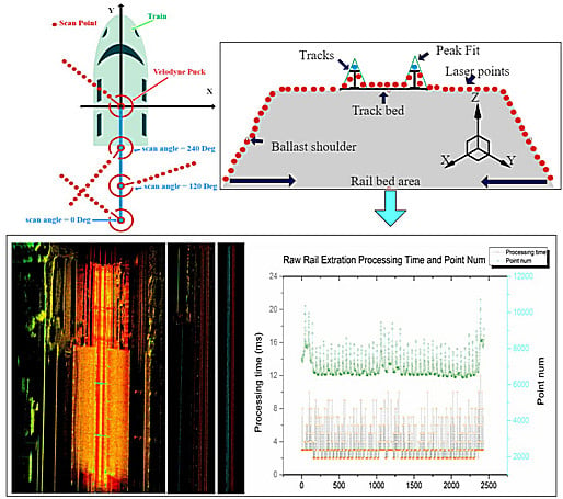
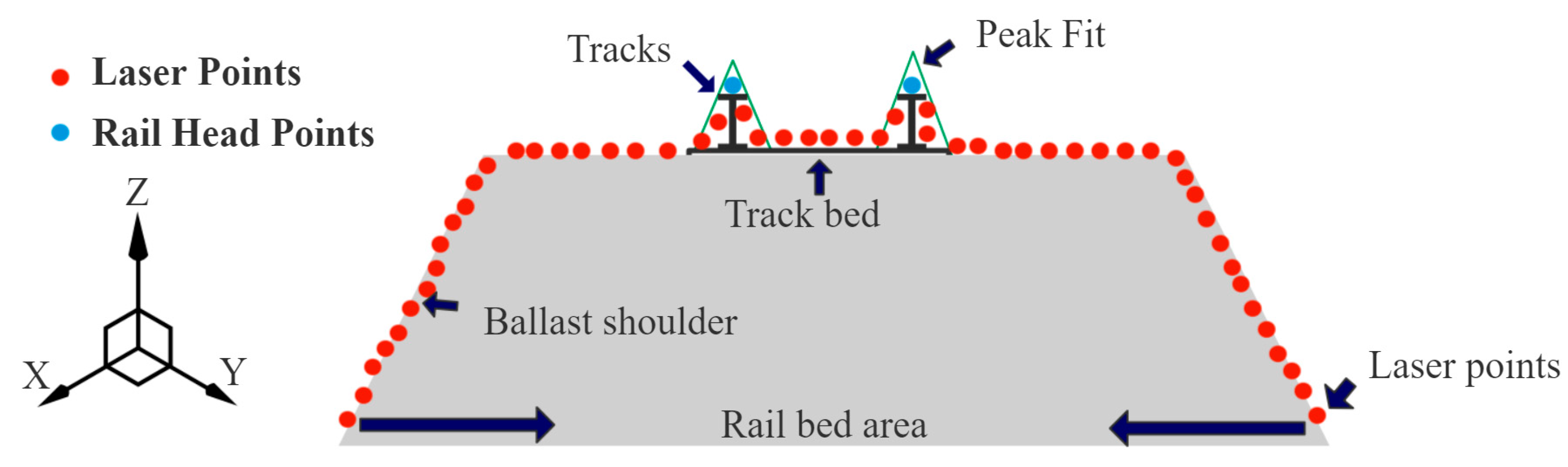
The tracks appear as thin and long lines in pairs in the MLS point cloud data. The tracks have low reflectivity to the laser used in the MLS system (usually infrared rays with a wavelength of around 905 nm), and the intensity value are generally small (regardless of measuring distance and angle of incidence). Thus, the tracks appear as a homogeneous strip [24]. The track is laid on relatively flat areas. The track bed is the surface below the track and topped with a ballast. The ballast comprises hard particles of uniform size and maintains the shape of the tracks (Figure 1).
In general, the rails have three major characteristics that distinguish them from other structures of the railway.
- The points on the rails show a protrusion on the scan line, which is similar to a mountain peak. In the local area of the mountain peak, the height difference is generally between 10 and 30 cm. The elevation rapidly increases and decreases in two main areas. Outside the two areas, the elevation changes are relatively flat.
- In the small circular area where the angle of incidence is approximately the same, the value of the intensity of the rail is smaller than that of the hard particle on the rail bed. This feature can be used in conjunction with the features mentioned in 1.
- Rails are generally located below the center of LiDAR, and the vertical distance from LiDAR is generally around 3–6 m (depending on the size of the scanning device and the train model on which the device is mounted).
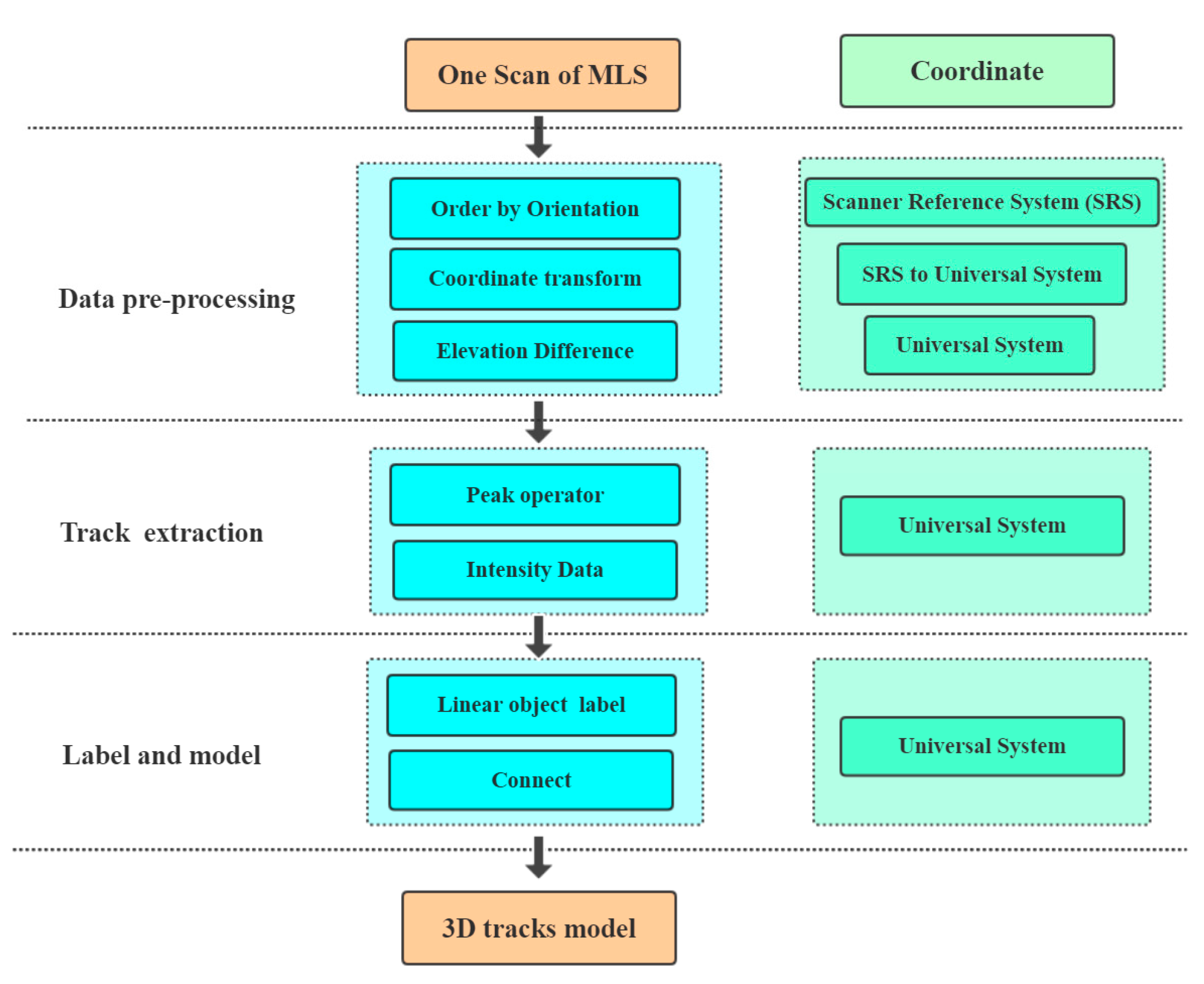
On the basis of the aforementioned information, we design a set of algorithms to achieve fast, automated extraction of rails, as shown in Figure 2.
The MMSs use the laser ranging principle to measure the distance. Combined with the orientation information generated inside the instrument, the coordinates of the measuring point in the LiDAR coordinate system can be obtained.
In different orientations, the distance between the detected object and LiDAR differs. The echo arrival times of the lasers previously emitted in chronological order cannot be maintained. As a result, the point cloud data are disorganized.
3.1. Data Preprocessing
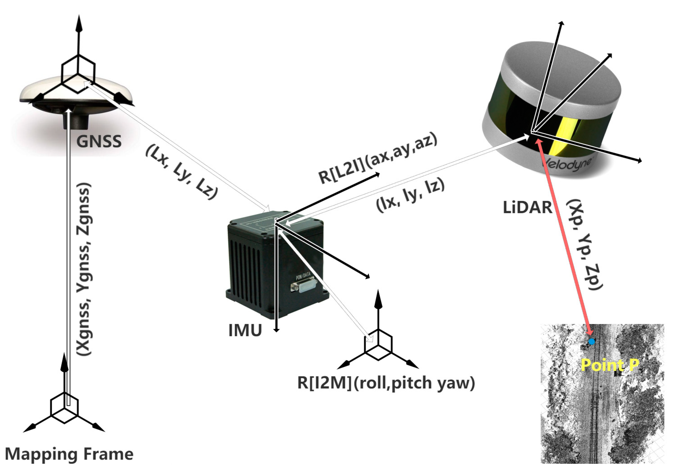
The data preprocessing section includes the following parts. The first part is the sorting of the original point cloud data. The points on each scan line are sorted according to the signal transmission time. This part is vital to avoid large-scale neighborhood calculations. Two coordinate systems are used in this step; one of them is the LiDAR coordinate system. Using the position, velocity, and attitude results (based on LiDAR Center) generated by the navigation unit (GNSS and IMU), coordinate transformation is performed to obtain the coordinates of each point in the local navigation coordinate (Easting, Northing, and Elevation) system, as shown in Figure 3. In this way, the elevation value of each point on the scan line can be obtained. On this basis, the sequence of elevation differences on the scan line can be derived.
A Velodyne puck is used for scanning. First, the vertical azimuth calculation for each point is performed on the basis of its coordinates in the LiDAR coordinate system, and which the scanning line Li {i = 0, 1, … 15} each point belongs to is determined depending on the azimuth angle. Then, the invalid points will be excluded (the distance measurement is infinity or 0). Vertical azimuth of every point Pi {xi, yi, zi} is calculated using Equation (1). This value is compared with the azimuth value of each scan line Ai {i = 0, 1, … 15} (provided in Velodyne specifications) to determine which line the point belongs to.
Thereafter, horizontal angle value HAi of every single point Pi {xi, yi, zi} will be calculated to determine the order in every scan line using Equation (2).
When the Point Cloud Data Are Sorted According to the Horizontal Angle, Coordinate Transformation Is Performed on Each Point in the Point Cloud to Obtain the Coordinates in the Geographic Reference Coordinate System [39].
The specific coordinate transformation formula is expressed as follows:
In Equation (3), [Xp, Yp, Zp]T presents the coordinate of target point P in certain mapping coordinate; [XGNSS, YGNSS, ZGNSS]T denotes the coordinate of GNSS antenna in the same mapping coordinate; denotes the rotation matrix from IMU frame to mapping frame; roll, pitch, and yaw are angles between IMU and mapping frames; presents the rotation matrix from LiDAR frame to IMU frame; ax, ay, and az are angles between LiDAR and IMU frames. The specific information is described in detail in Table 1.
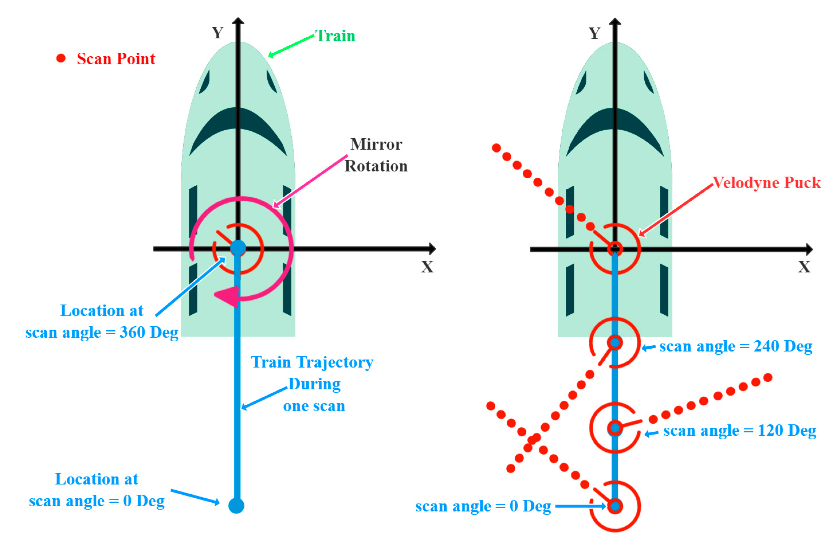
Although all parameters have been given, there is one more problem that should be taken into consideration. Laser scanners continuously emit laser pulses and digitize return pulses. In practice, compared to the speed of light, the moved distance of the laser scanner at a given scan angle could be neglected (e.g., assume the distance between object and laser scanner is 100 m, the moving speed of laser scanner is 20 m/s, then the calculated movement during light travel time will be 0.000013 m). However, Figure 4 presents that the movement of a laser scanner between different scan angles could cause oversampling [40,41] and distortion in point cloud data.
GNSS/INS trajectory is used to remove motion-based distortion [42] within the scan. According to Equation (2), start angle and end angle could be calculated for the first and last return point in one scan, respectively. Then, trajectory of GNSS antenna [XGNSS, YGNSS, ZGNSS]T is interpolated in accordance with given location at start scan angle and end scan angle. Besides, the rotation matrix is calculated in accordance with angles from IMU output. [XGNSS, YGNSS, ZGNSS]T and update in Equation (3) at every scan angle. By means of that, the corrected scan could be transferred to next step for track extraction. This procedure is based on two conditions: one is no relative movement between the GNSS and laser scanner at one quick scan; the other is that the train trajectory is a straight line during one scan.
When the aforementioned sorting and coordinate transformation steps are completed, the elevation difference value on each scan line will be calculated using Equation (4).
Notably, in many rail areas, the train will change direction. To meet the speed requirements of the train, the elevations on the sides of the rails appearing in pairs will be different; one side is slightly higher, whereas one side is slightly lower. In this case, the sliding window method proposed by Yang et al. [24] may fail because the track bed will also have a corresponding elevation change.
3.2. Track Extraction
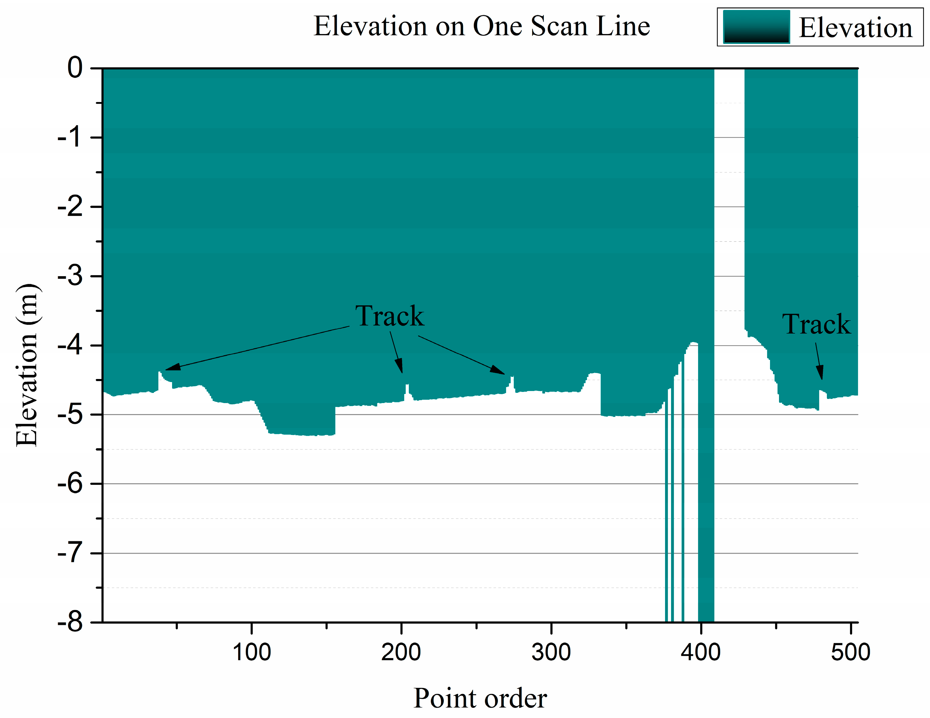
To vividly describe the process of rail extraction, an elevation map above a scan line will be given and sorted according to the orientation in which it appears.
In Figure 5, the example data are acquired on a bridge, with the elevation of the coordinate origin of the LiDAR coordinate system being 0 and that below the origin of the coordinate being negative. The figure shows four peaks raise up and jump suddenly. The four peaks have two major characteristics that distinguish them from other points.
- Notably, standard rail height is 15.9 cm. In Figure 6, cumulative elevation differences at four peaks on both sides is between 30 and 40 cm.
- Elevation changes at left and right neighbor of these peaks are slight.
As shown in Figure 6, the point above the track has three characteristics:
- The height difference between the point above the track and the adjacent sampling point is between 10 and 30 cm, and the height difference of the track bed is between 1 and 2 cm. Equation (5) is used to determine whether the point Pi {Xi, Yi, Zi} belongs to the track point set .
- After the MLS is installed, the difference in elevation between the track and the scanner center is roughly determined. In this experiment, the set thresholds Eup and Edown are −3 and −6 m, respectively. Equation (6) is used to decide whether the previous point should be excluded from the point set .
- The track candidate point is the center, and the elevation changes on the left and right sides show a pattern of increase and decrease, which is similar to a peak. The number n of points used is 10 in calculating the cumulative difference of the elevations on both sides. The accumulated difference value is less than the limit value R. The threshold R used in this case is 155 mm, which is consistent with that adopted by Yang et al. [24].
When the point meets the above-mentioned conditions, it must be adjusted according to the value of intensity. The points of misjudgment can be eliminated because steel and rail beds exhibit different reflection characteristics. The main practice is to perform the same calculation above for the difference sequence of intensity. is the accumulated difference value of intensity. Otherwise, points can be excluded from the point set .
However, apart from stones of uniform size, steels are present on the track bed. The intensity values of these materials are similar to those of tracks, and some exhibit similar geometries to those of the rails. The scanning line has a wide scanning range, and the features in the plain area are false negatives, which require further filtering. The specific operation is described in detail in the following subsection.
3.3. Label and Model
After the above steps, the extracted points are mostly the points above the rails, except for some outlier points whose geometry and reflection modes are similar to those of the rails.
Ideally, if the rails are sampled evenly, principal component analysis (PCA) could be applied to the point cloud for each frame. Then the largest eigenvector determines the perpendicular projection direction, and each point is projected into the direction. The projection length can be used to cluster the points to realize the distinction between the rails.
However, due to the uncertainty of noise, the projection direction is poor when principal component analysis is performed. As far as the projection length is concerned, the point clouds from different rails are mixed and cannot be quickly distinguished.
In the case of a Velodyne puck at 10 Hz, two pairs of rails are assumed to be present, and each frame can capture up to 64 rail track head points. To ensure that the point cloud is sufficiently dense, the candidate points collected above are clustered in accordance with the Euclidean distance analysis rule after accumulating 10 scans of point clouds P. Specific steps are listed as follows:
- Create a Kd-tree representation for the input point cloud dataset P.
- Set up an empty list of clusters C and a queue of the points that need to be checked Q.
- For every point pi that belongs to P, perform the following steps:
- Add pi to the current queue Q.
- For every point pi that belongs to Q, search for the point neighbor set of pi in a sphere with radius r < 0.7. For every neighbor point in the set, check if the point has already been processed; if not, add it to Q.
- When the list of all points in Q has been processed, add Q to the list of clusters C and reset Q to an empty list.
- The algorithm terminates when all points pi in P have been processed and are now part of the list of point clusters C.
The radius threshold of neighbors r is selected considering the track gauge (1.435 m) to exclude points from adjacent rail tracks. For every cluster ci in C, we perform the following steps to detect rail track and filter outliers.
- ci with fewer than 10 points will be filtered, which will rule out most of the false negatives.
- For points pi = [xi, yi, zi]T i = 1, 2, …, k in ci, 3D PCA is used to obtain local covariance matrix M.
- M is symmetric positive semi-definite [24], and has non-negative eigenvalues. The three eigenvalues of M are positive and ordered as . Those clusters with no dominant direction can be detected . Those planes will be filtered according to . Those clusters with will be detected as linear features. This step is called PCA filter, as shown in Figure 7. Using mentioned in previous work [26] where
These linear clusters are connected using the region growing method, and this step produces many lines that are parallel to one another. A track may comprise multiple discrete lines due to occlusion during the acquisition process.
The final extraction goal is to achieve object level identification. That is, each pair of rails will be distinguished as the final unit of identification.
This step is accomplished in accordance with the Euclidean distance analysis rule, whereas the radius threshold of neighbors r1 = 1.435 is selected considering the track gauge (1.435 m). In this way, points belonging to the same pair of rails will be extracted, thereby realizing the extraction of the rails.
4. Environment and Data Description
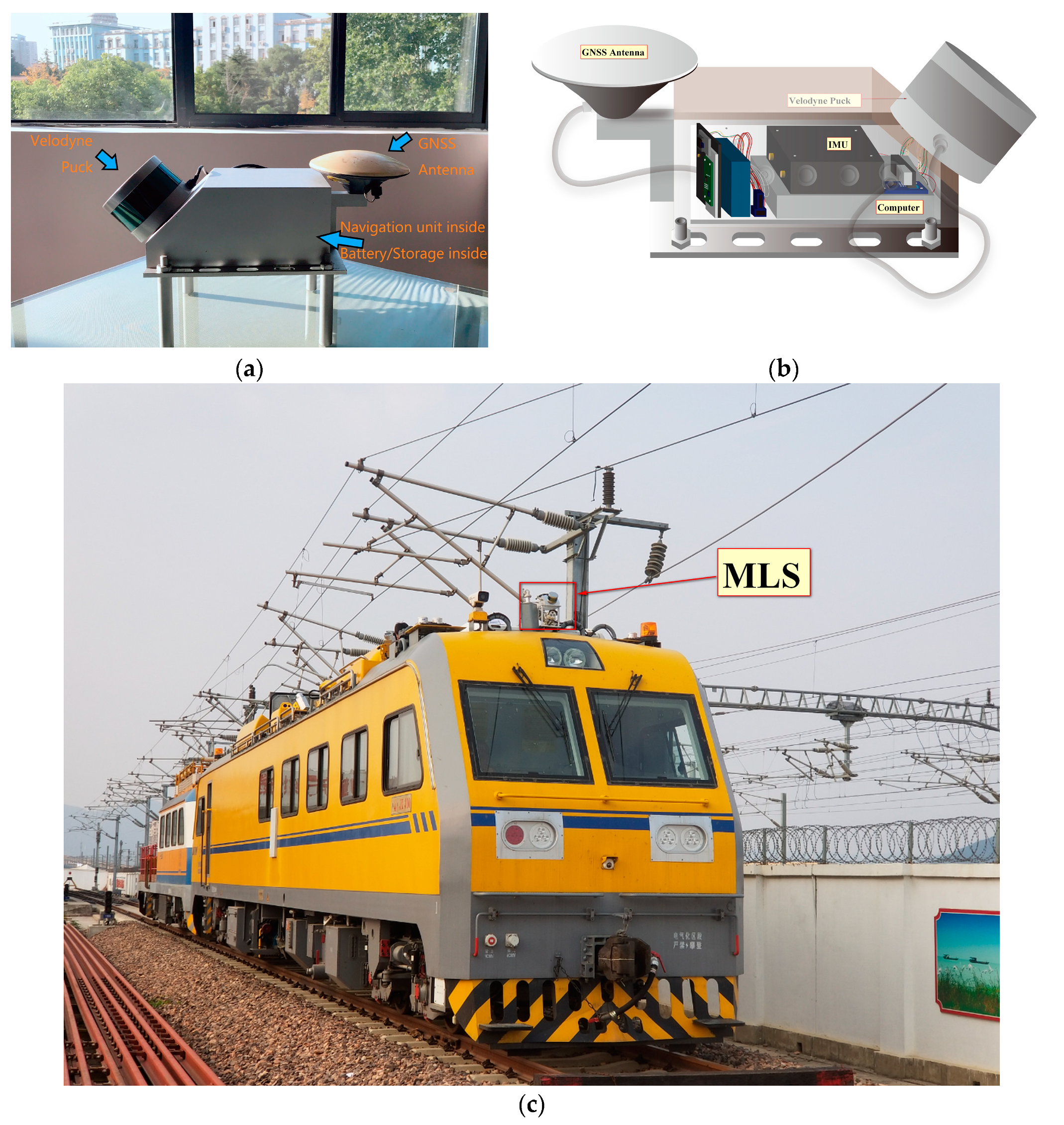
The experiments are conducted with one hour observation data collected on the midnight of 28 May 2018 (started at 15:30 UTC). Data acquisition equipment includes the Velodyne puck, navigation unit, GNSS receiver, and data storage computer, as shown in Figure 8a,b. Travel length is 40 km. The data acquisition device is mounted on top of the railcar with an open top view, as shown in Figure 8c.
The navigation unit of this MLS contains an integrated GNSS/INS system. Table 2 shows the specifications of the product in detail.
The parameters used to describe the relative relationship between the GNSS/IMU/LiDAR sensors of the system are explained in detail in Table 1 and Figure 3.
As shown in Figure 8, LiDAR equipment is not placed horizontally to increase the number of echo points. Specification of LiDAR used in this study is provided in Table 3.
4.1. Position Accuracy Description
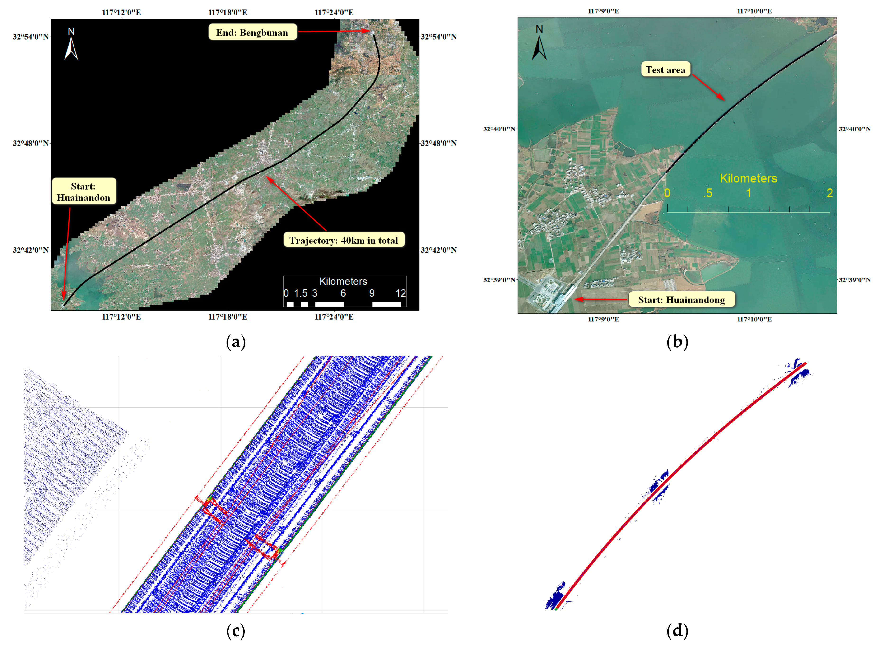
We use a satellite image with no offset as the base map to intuitively illustrate the general test area. The calculated position is plotted on the base map, as shown in Figure 9.
In Figure 9a, the train trajectory, starting point, and end point are marked with a total length of 40 km. In this paper, the MLS system was initialized outside the train station before the experiment began. The train then entered the train station and stayed for a while. Later, the train left the platform and traveled 40 km in the open area to another train station. The portion for rail extraction and statistical analysis is shown in Figure 9b. In addition, to examine the applicability of the proposed method in a poor GNSS observation environment (e.g., satellite numbers less than four and no GNSS signals), a rail extraction experiment was performed using the data collected by the MLS system when the train just entered the station.
The start point is near one railway station, as shown in the lower left side in Figure 9a.
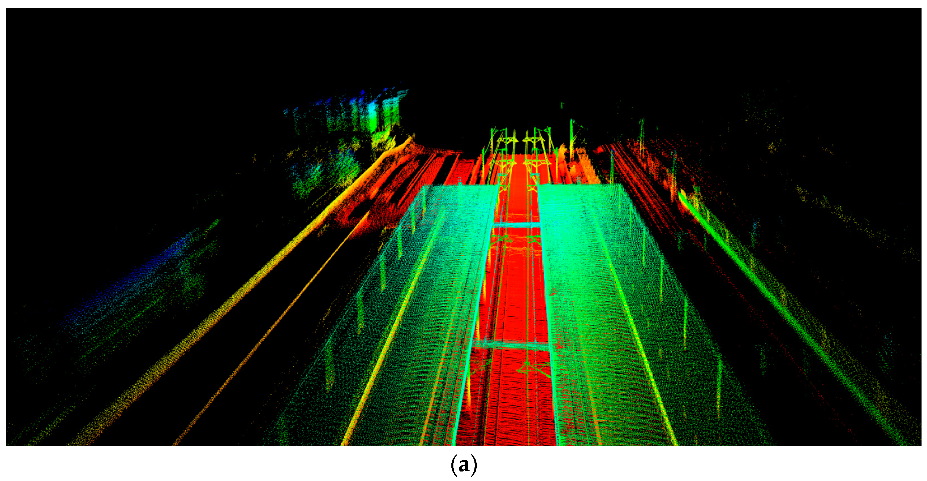
Inside the train station, the GNSS antenna cannot receive the satellite signal due to the obstruction at the top of the platform. Therefore, the MLS system cannot obtain the GNSS antenna position information. In the absence of GNSS observations, only the observations of the IMU can be used for dead reckoning, and the position accuracy is worse than the GNSS/INS combination result. Until the GNSS antenna receives a reliable GNSS signal, the MLS system uses GNSS and IMU observation data for comprehensive processing. As a general rule, when the positional accuracy is below the threshold, the MLS system stops recording data [43] or records the data but does not process it. Figure 10a–b shows the point cloud results of the MLS system output when the train just entered the station, colored by elevation and intensity, respectively.
As shown in Figure 10a,b, the train station has four pairs of rails. The GNSS signal was blocked when the train entered the station. Rail extraction results without GNSS signals are given in Figure 10c–f. Figure 10c presents the top view of the point cloud in the train station area. The outputs of track extraction step, label and model step are shown in Figure 10d,e, respectively. Figure 10f presents that two pairs of tracks are correctly recognized. Results show that our method is capable of extracting rail data with several seconds of loss of the GNSS signals.
However, the other two pairs of rails are not extracted. Reasons and suggestions are given in Section 5.2.
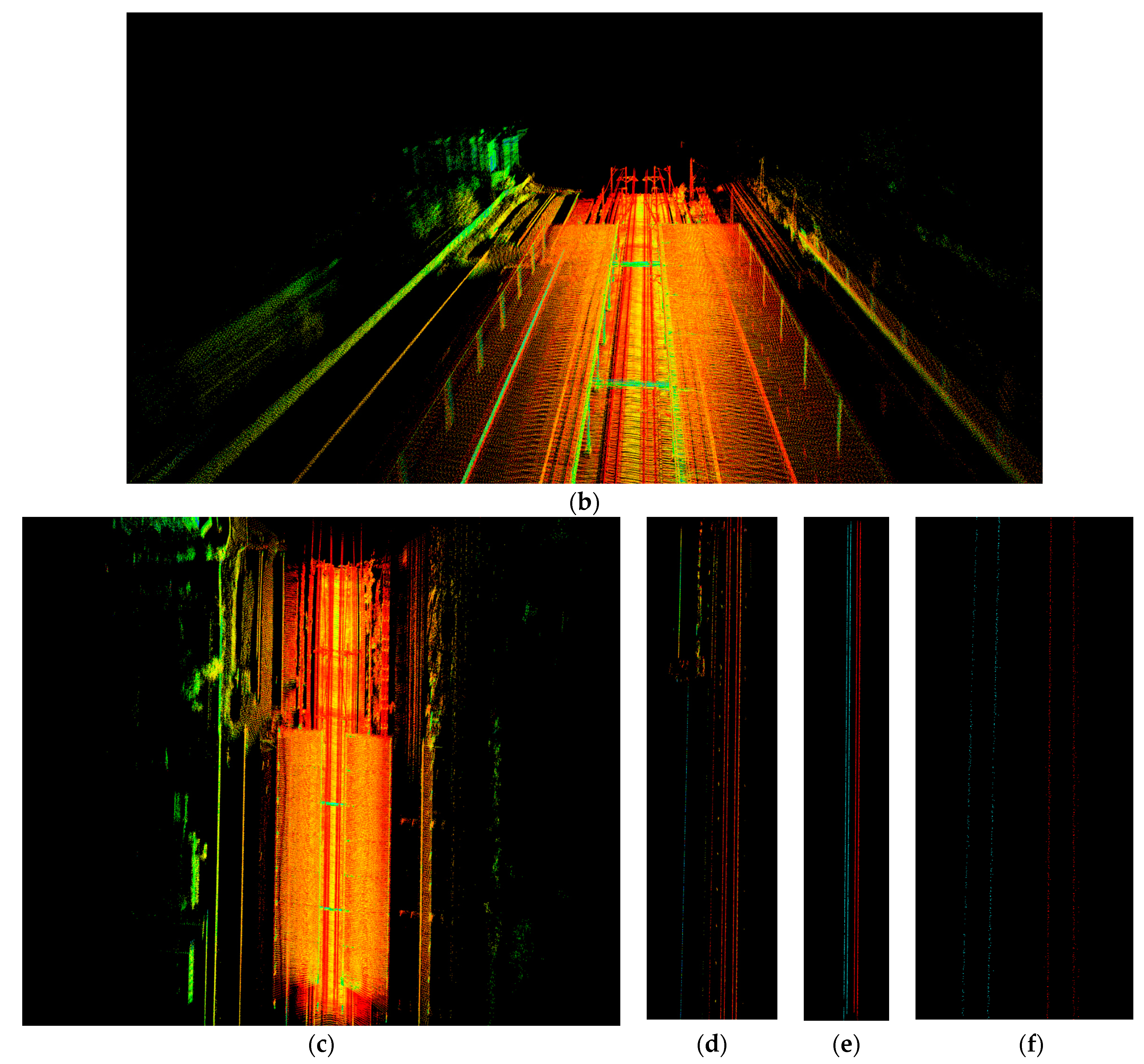
Through processing, the GNSS/INS data collected in the open area are statistically analyzed. Figure 11 shows that the positioning STD results in centimeter level in all three directions.
The following is a brief introduction to the test area (Shown in Figure 9b–d) for rail extraction and analysis.
4.2. Test Area Information
The planimetric size of the test rail extraction area is 1618 m × 1651 m with a height variation of 96.06 m. Test trajectory length is 2.21 km. Figure 9d demonstrates an overview of the test data, and Figure 9c provides a close-up top view of a portion of the data, which is colored by elevation. The data contains spatial information and the intensity field. Given that the data collection began at 15:30 UTC, and the artificial light source is insufficient to meet the requirements of the RGB camera. Therefore, the MLS data records only contain 3D coordinates and intensity. The test data contain 17 million points in total with a mean point density of approximately 490 points per square meter. The proposed method is implemented as a tool for fast, automated rail extraction.
The real-time feasibility evaluation of the test algorithm is completed in the simulation environment, which is built based on the ROS. Test data are also processed using an i5 computer. The outputs of the tool are exported in Terrasolid and a PCL [44] viewer for decent visualization.
5. Results and Discussion
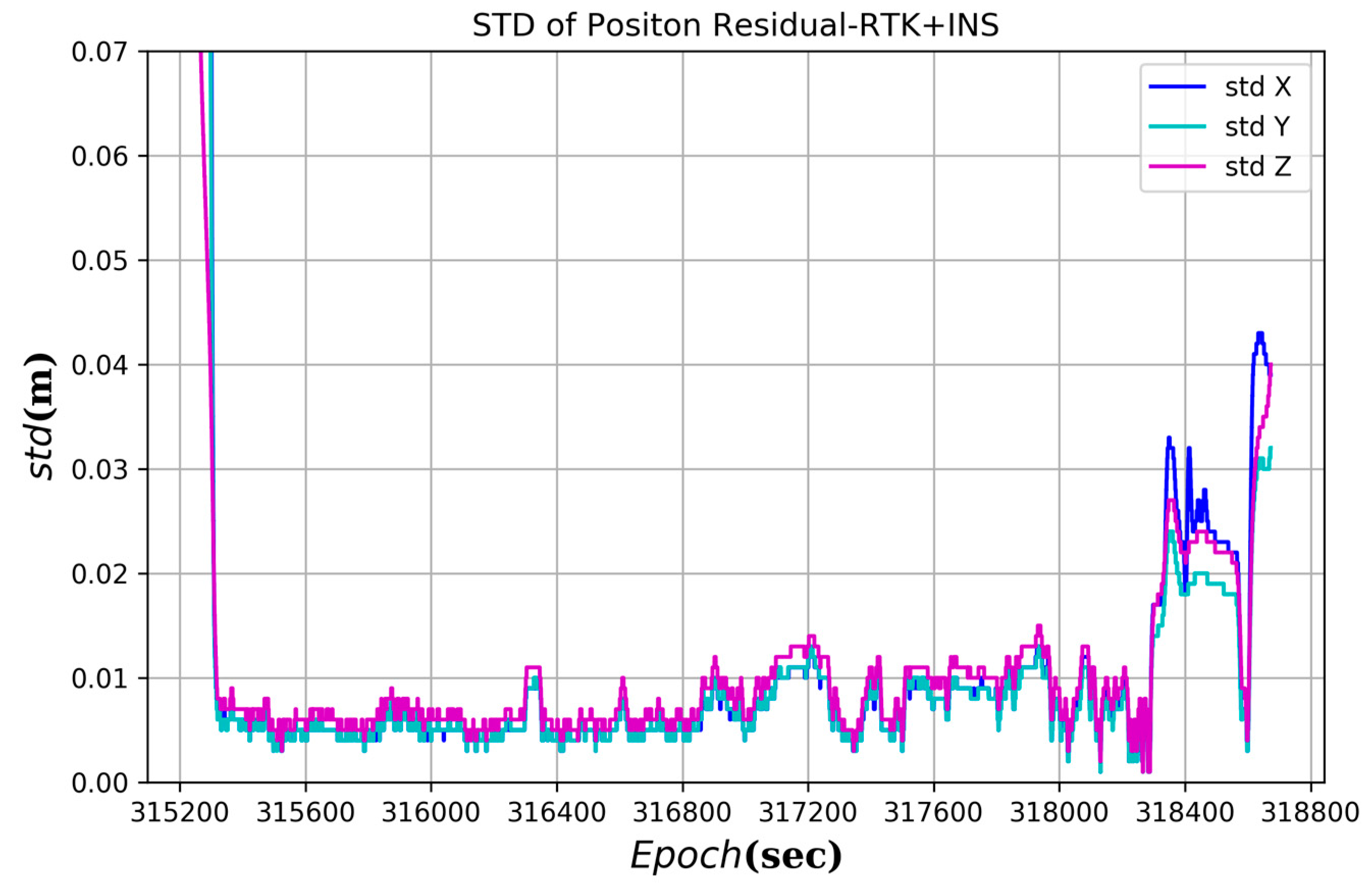
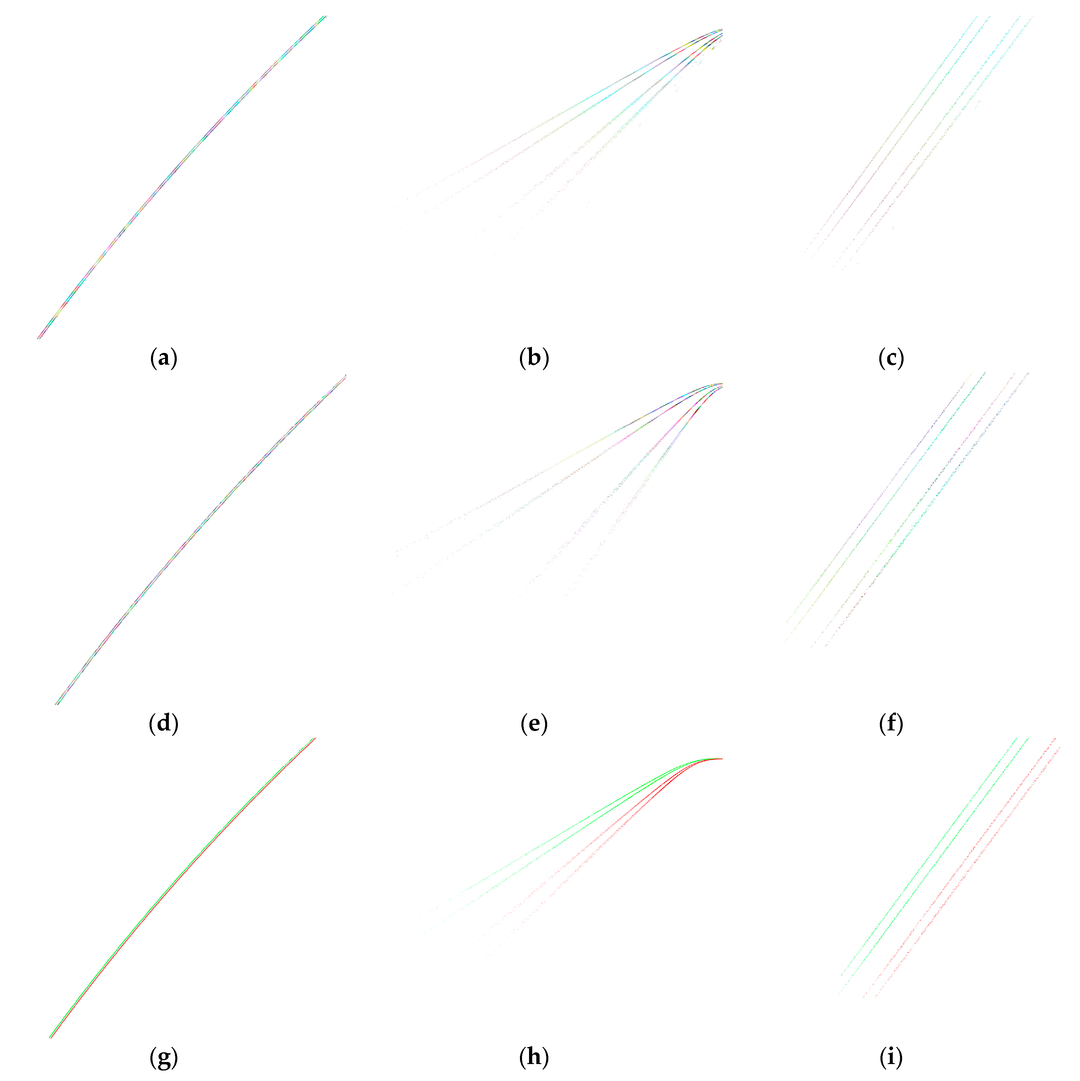
The simulation environment is built using the robot operating system (ROS). The raw data captured by the MLS platform are played back at 10 Hz. In each scan line, points are ordered by the orientation in the LiDAR coordinate. For each scan, points from local LiDAR coordinate systems are transformed to a local navigation coordinate (Easting, Northing, and Elevation) system by using the provided GNSS/INS solution. Thus, their height differences are calculated for rail head extraction, as shown in Figure 12a–c (random color for points). Results show that the proposed method works well in rail head raw extraction.
The standard track gauge is 1.435 m. The MLS system is approximately 3 m higher than the rail bed. Notably, the railway in the experimental area is designed to be curved. To meet the centrifugal force required for the train to turn, a certain height difference is applied on both sides of the same pair of tracks. In line with the aforementioned information, certain parameter thresholds are empirically selected for the proposed method, as listed in Table 4. Most rail head points in one scan are detected using the peak geometric patterns and the intensity difference.
Some false positives, such as structure points of mass, are in scattered distribution. For 10 scans in 1 s, the candidate points are clustered using the region growing method, and the number of points in the cluster less than 10 will be filtered out. After PCA is performed for each cluster, the scattered cluster will be deleted. The processed result after the PCA filter is shown in Figure 12d–f (random color for points). The results show that scatter points are discarded, and rails with linear distribution in every second are correctly labeled.
The ultimate goal of rail extraction is to obtain pairs of rail tracks. The region growth method is again used with a different neighbor radius r1, and rails that belong to the same pair will be connected and labeled. Figure 12g–i (color by track index) shows different views of recognized pairs of the test area.
5.1. Timing for Key Extraction Steps
This work aims to propose a rail extraction approach for LiDAR data that is fast and easy to implement, runs at 10 Hz, and provides high-quality results. Experiments are designed to show the capabilities of the proposed method and support key claims that this method can be executed fast even on a simple i5 computer with at least 10 Hz for a Velodyne puck.
In assessing the time consumption of each critical step in the rail extraction, the entire extraction process is divided into two parts. The first part is the preliminary extraction process of the track as discussed in Section 3.2; this step is the raw rail extraction. The other part is the Euclidean distance cluster and a PCA filter, as discussed in Section 3.3; this step is the PCA filter.
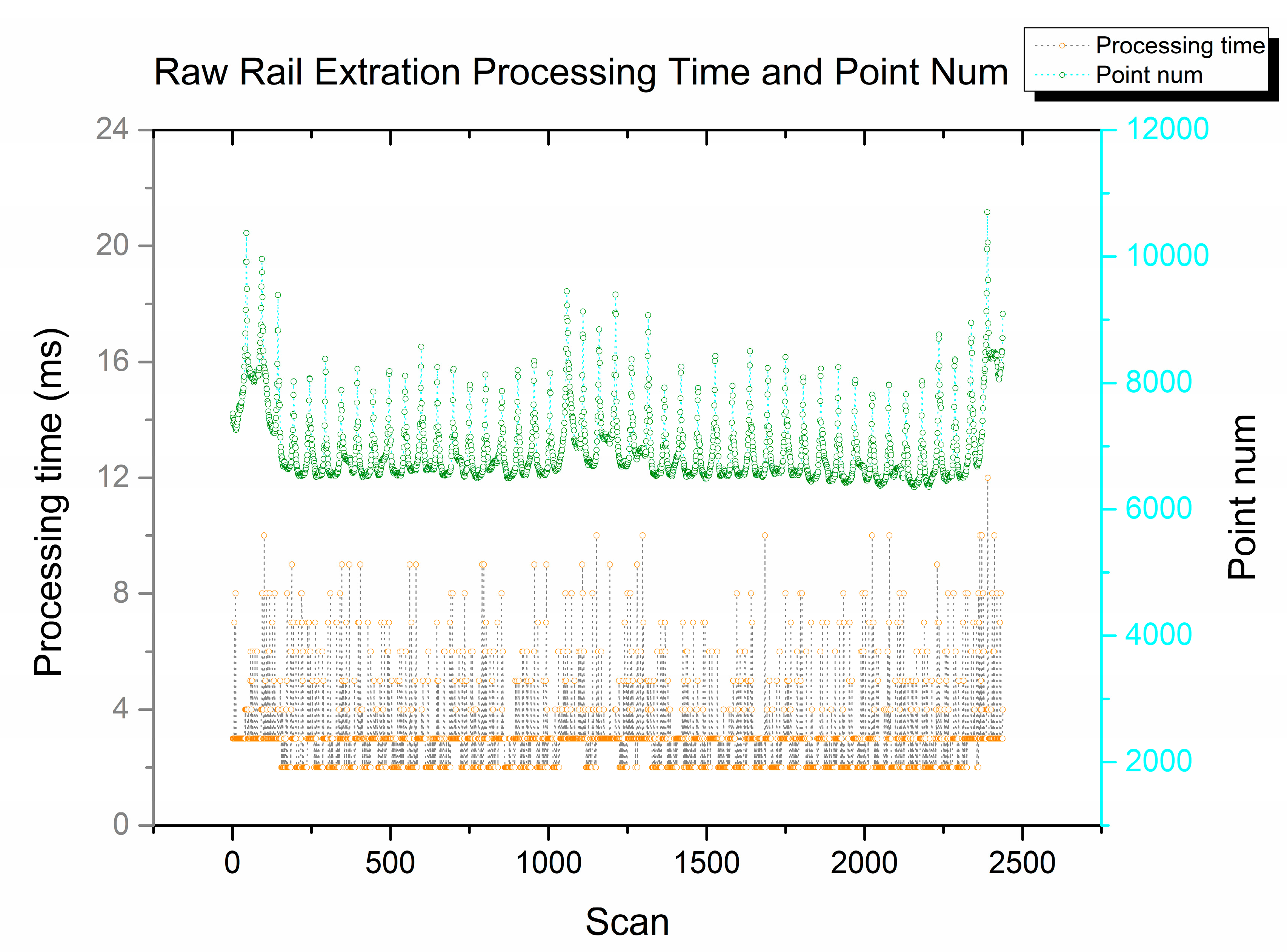
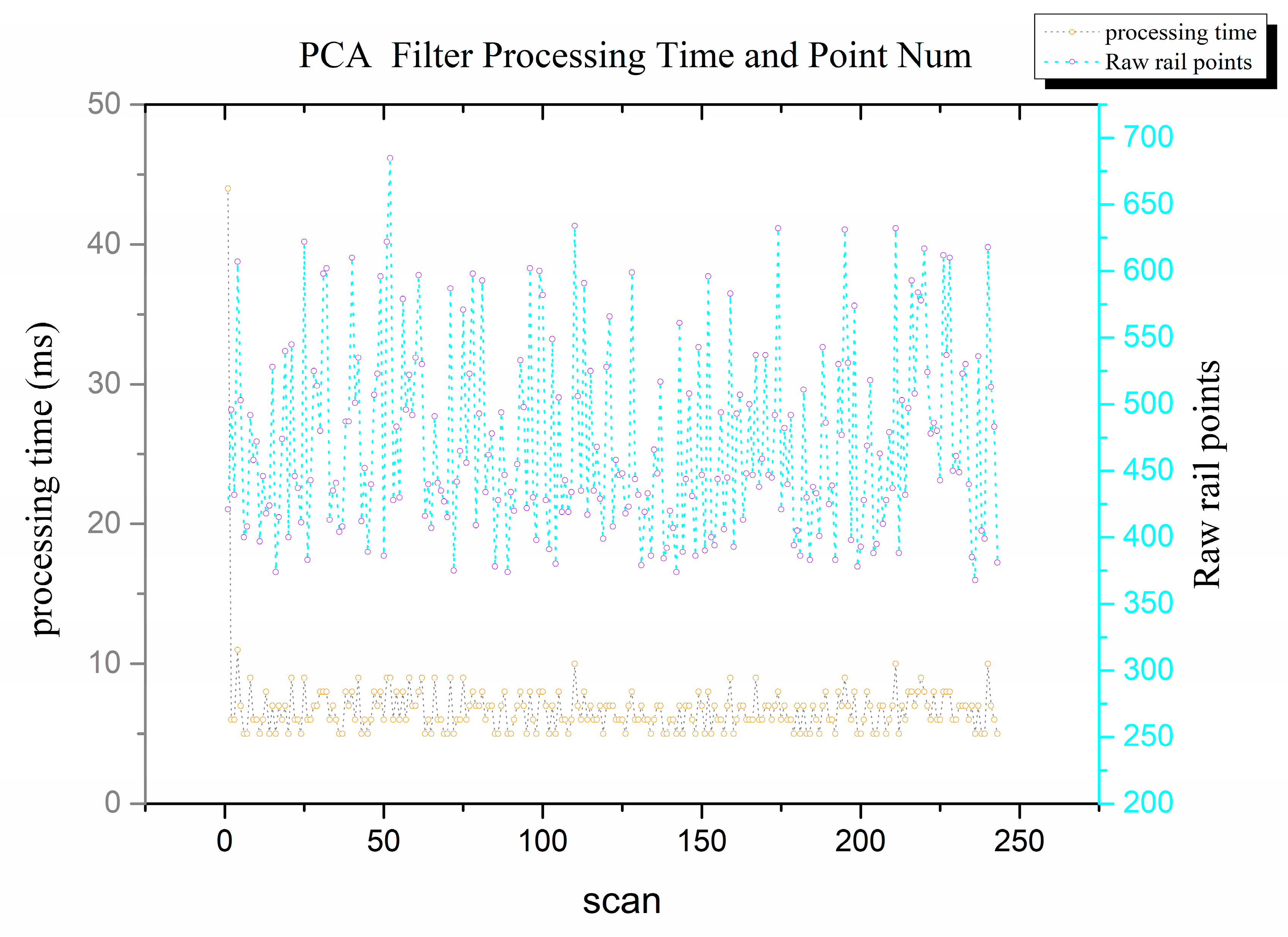
With the provided GNSS/INS solution, the raw data captured by the LiDAR under the ROS are played back and run at a frame rate of 10 Hz. The time spent in each of the two steps and the total number of points processed are counted. Double Y-axis graphs are plotted for processing time and a number of points in each step, as shown in Figure 13 and Figure 14, respectively.
The raw rail extraction step consumes less than 12 ms per scan while processing more than 6000 points on average. For an interval of 100 ms per scan, the processing time is approximately equal to one-tenth. Therefore, as long as the GNSS/INS provides accurate positions and pose information within 90 ms, the track can be initially extracted for further processing.
In the PCA filter step, 10 scans in 1 s will be processed simultaneously while discrete points and false positives are removed. Clustering and PCA consume 10 ms. After the previous step, the number of extracted rail points is greater than 350 points.
In summary, the proposed approach can be used in fast rail extraction when GNSS/INS solutions are provided. In the following subsection, the quality of the extracted tracks is evaluated.
5.2. Quantitative Evaluation of Rail Extraction
The resolution of high-quality satellite image for civil use is limited to only up to 0.6 m per pixel due to national policies. This condition indicates that decent visual comparison cannot be presented given that the standard track gauge is 1.435 m per 2 pixels in Google Earth imagery.
The achieved results are assessed by manual delineation of rails (reference data). The basic traits of the standard rail are 140 mm in width at the foot, 70 mm in width at the rail head in test area. We created the buffer zones with width of 35 mm around the manually digitized lines (considered as ground truth), and then we compared the extract rails with reference data. Figure 12g presents the recognition results, which indicate that two pairs of tracks are recognized correctly. The assessment is carried out at point cloud level. Analysis results are shown in Table 5, at the point cloud level, precision, accuracy and sensitivity are computed using Equations (12)–(14).
where denotes the number of true positive points, which is the number of rail points found in both ground truth and detected data. is the number of true negative points, which is the number of points that were in neither ground truth nor detected data. is the number of false positive points, which is the number of points that were detected but did not exist in ground truth. denotes the number of false negative points, which is the number of rail points found in ground truth but were not found in detected data.
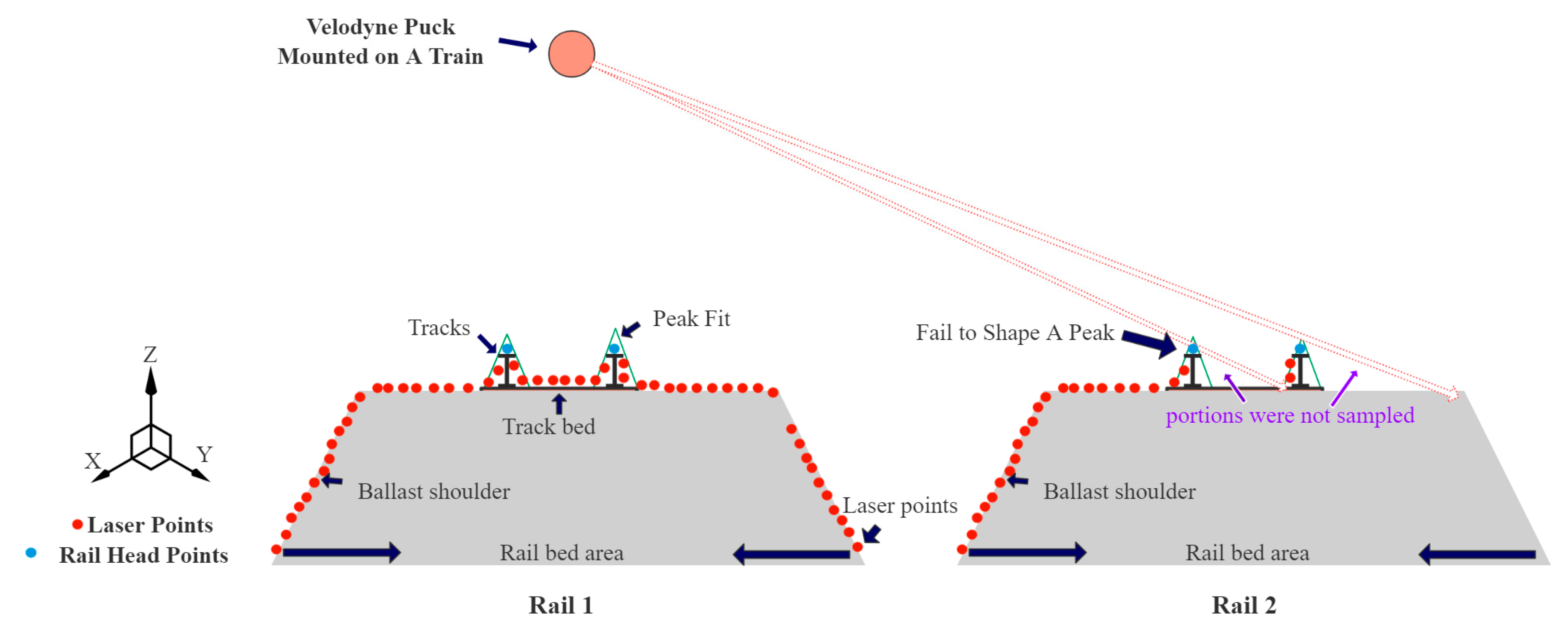
Accuracy, precision, and sensibility of the total test area are 99.68%, 97.55% and 66.55%, respectively. Many rail points are undetected in Pair 2 because the rail car runs at Pair 1, as shown in Figure 15. In this case, occlusion is the main cause for failure (same in Section 4.1) at some portions. The peak shape of Pair 2 is unrecognizable, which contributes to most false negatives in Pair 2. Therefore, at a multi-track area (e.g., 8 pairs and 16 pairs of tracks), a close collaboration between MMSs mounted on several trains is required.
6. Conclusions
The spatial data information of railroad tracks is important to railway shift arrangements, passenger comfort, and railway safety. This study presents a method for fast fully-automated recognition of rail pairs using LiDAR data collected by MLS system. The data are acquired by MMS developed by the authors, which is mounted on a railcar operating at 40 km/h. The results show that positioning STD is lower than 4 cm in most areas. Test data contain 17 million points in total with a mean point density of approximately 490 points per square meter.
We perform several experiments at key steps of rail extraction by using ROS as a simulation environment. When geometric pattern and intensity characteristics of rail tracks are combined, extracting raw rail head points per scan from greater than 6000 points consumes less than 12 ms using an i5 computer with a sampling rate of 10 Hz. At PCA filter step, which will be executed every second, scattered clusters are removed in less than 10 ms. These results imply that the proposed method can be run in real-time at 10 Hz for a common MLS system if GNSS/INS solutions are provided in time. The proposed method correctly recognizes two pairs of rail tracks and performs well in no GNSS signal environment. At the point cloud level, accuracy, precision, and sensitivity of the total test area are 99.68%, 97.55% and 66.55%, respectively. Occlusion is the main cause of failure at some portion. Thus, at a multi-track area (e.g., 8 pairs and 16 pairs of tracks), close collaboration between MMSs mounted on several trains is required.
This study demonstrates the feasibility of extracting rail tracks in real time from MLS data. Consequently, we will investigate the application of spatial rail data in the inspection and maintenance of rails. According to conventional wisdom, 3D models can provide a user-friendly interface and require less storage. Thus, we will explore the modeling of railway infrastructures in real time.
Author Contributions
Conceptualization, Y.L., T.Z. and J.T.; Methodology, Y.L. and T.Z.; Software, T.Z.; Validation, Y.L., T.Z. and W.S.; Formal analysis, Y.Z.; Resources, Y.L., J.T. and W.S.; Data curation, L.C.; writing—original draft preparation, Y.L. and T.Z.; Writing—review and editing, Y.L., T.Z., J.T. and W.S.; visualization, T.Z.; Supervision, Y.L. and W.S.; Project Administration, Y.L. and W.S.
Funding
This research was partially supported by State Key Research and Development Program of China (Grant No. 2017YFB0503401, Grant No. 2016YFB0501802), National Natural Science Funds of China (Grant No. 41704026, Grant No. 41374034, Grant No. 41404010), and also by Open Research Fund of State Key Laboratory of Information Engineering in Surveying, Mapping and Remote Sensing (Grant No. 15P01).
Acknowledgments
Yongfeng Zhang and Yuhan Qin from Wuhan University, China are highly appreciated for collecting the data.
Conflicts of Interest
The authors declare no conflict of interest.
References
- Yu, X.; Lang, M.; Gao, Y.; Wang, K.; Su, C.; Tsai, S.; Huo, M.; Yu, X.; Li, S. An Empirical Study on the Design of China High-Speed Rail Express Train Operation Plan—From a Sustainable Transport Perspective. Sustainability 2018, 10, 2478. [Google Scholar] [CrossRef]
- Ma, L.; Li, Y.; Li, J.; Wang, C.; Wang, R.; Chapman, M. Mobile Laser Scanned Point-Clouds for Road Object Detection and Extraction: A Review. Remote. Sens. 2018, 10, 1531. [Google Scholar] [CrossRef]
- Genderen, J.L.V. Airborne and terrestrial laser scanning. Int. J. Digit. Earth 2010, 4, 183–184. [Google Scholar] [CrossRef]
- Novak, K. Integration of a GPS-receiver and a stereo-vision system in a vehicle. In Proceedings of the SPIE—The International Society for Optical Engineering, Zurich, Switzerland, 3–7 September 1990; pp. 16–23. [Google Scholar]
- Zumberge, J.F.; Heflin, M.B.; Jefferson, D.C.; Watkins, M.M.; Webb, F.H. Precise point positioning for the efficient and robust analysis of GPS data from large networks. J. Geophys. Res. 1997, 102, 5005–5017. [Google Scholar] [CrossRef] [Green Version]
- Parkinson, B.W.; Enge, P.; Axelrad, P.; Spilker, J.J., Jr. Global Positioning System: Theory and Applications, Volume II; American Institute of Aeronautics and Astronautics: Washington, DC, USA, 1996. [Google Scholar]
- Barreiro, J.B.; García, F.A.V.; Mora, P.M.V.; González, R.C.L. Aplicación de Sistemas GNSS y SIG a Infraestructuras de Transporte: Estudio Sobre la Conducción Naturalista; Universidade da Coruña: Galicia, Spain, 2015. [Google Scholar]
- Guan, H.; Li, J.; Cao, S.; Yu, Y. Use of mobile LiDAR in road information inventory: A review. Int. J. Image Data Fusion 2016, 7, 219–242. [Google Scholar] [CrossRef]
- Wang, H.; Luo, H.; Wen, C.; Cheng, J.; Li, P.; Chen, Y.; Wang, C.; Li, J. Road Boundaries Detection Based on Local Normal Saliency From Mobile Laser Scanning Data. IEEE Geosci. Remote. Sens. Lett. 2015, 12, 2085–2089. [Google Scholar] [CrossRef]
- Kumar, P.; Lewis, P.; McElhinney, C.P.; Boguslawski, P.; McCarthy, T. Snake Energy Analysis and Result Validation for a Mobile Laser Scanning Data-Based Automated Road Edge Extraction Algorithm. IEEE J. Sel. Top. Appl. Earth Obs. Remote Sens. 2017, 10, 763–773. [Google Scholar] [CrossRef]
- Kumar, P.; McElhinney, C.P.; Lewis, P.; McCarthy, T. An automated algorithm for extracting road edges from terrestrial mobile LiDAR data. ISPRS J. Photogramm. Remote Sens. 2013, 85, 44–55. [Google Scholar] [CrossRef] [Green Version]
- Zai, D.; Li, J.; Guo, Y.; Cheng, M.; Lin, Y.; Luo, H.; Wang, C. 3-D Road Boundary Extraction From Mobile Laser Scanning Data via Supervoxels and Graph Cuts. IEEE Trans. Intell. Transp. Syst. 2018, 19, 802–813. [Google Scholar] [CrossRef]
- Chen, X.; Li, J. A Feasibility Study on Use of Generic Mobile Laser Scanning System for Detecting Asphalt Pavement Cracks. In Proceedings of the ISPRS—International Archives of the Photogrammetry, Remote Sensing and Spatial Information Sciences, Prague, Czech Republic, 12–19 July 2016; pp. 545–549. [Google Scholar]
- Guan, H.; Yu, Y.; Li, J.; Liu, P.; Zhao, H.; Wang, C. Automated extraction of manhole covers using mobile LiDAR data. Remote Sens. Lett. 2014, 5, 1042–1050. [Google Scholar] [CrossRef]
- Campos-Taberner, M.; Romero-Soriano, A.; Gatta, C.; Camps-Valls, G.; Lagrange, A.; Le Saux, B.; Beaupere, A.; Boulch, A.; Chan-Hon-Tong, A.; Herbin, S. Processing of extremely high-resolution LiDAR and RGB data: Outcome of the 2015 IEEE GRSS data fusion contest—Part a: 2-D contest. IEEE J. Sel. Top. Appl. Earth Obs. Remote Sens. 2016, 9, 5547–5559. [Google Scholar] [CrossRef]
- González, A.; Villalonga, G.; Xu, J.; Vázquez, D.; Amores, J.; López, A.M. Multiview Random Forest of Local Experts Combining Rgb and Lidar Data for Pedestrian Detection; IEEE: Washington, DC, USA, 2015; pp. 356–361. [Google Scholar]
- Han, J.; Guo, J.; Jiang, Y. Monitoring tunnel profile by means of multi-epoch dispersed 3-D LiDAR point clouds. Tunn. Undergr. Space Techchol. 2013, 33, 186–192. [Google Scholar] [CrossRef]
- Morgan, D. Using mobile LiDAR to survey railway infrastructure. Lynx mobile mapper. Proc. FIG Comm. 2009, 5, 32–40. [Google Scholar]
- Leslar, M.; Perry, G.; McNease, K. Using mobile LiDAR to survey a railway line for asset inventory. In Proceedings of the ASPRS 2010 Annual Conference, San Diego, CA, USA, 30 July 2010; pp. 26–30. [Google Scholar]
- Kaleli, F.; Akgul, Y.S. Vision-based railroad track extraction using dynamic programming. In Proceedings of the International IEEE Conference on Intelligent Transportation Systems, St. Louis, MO, USA, 4–7 October 2009. [Google Scholar]
- Sawadisavi, S.; Edwards, J.R.; Hart, J.M.; Barkan, C.P.L.; Ahuja, N. Machine-Vision Inspection of Railroad Track. In Proceedings of the 2008 AREMA Conference, Salt Lake City, UT, USA, 21–24 September 2009; pp. 1–6. [Google Scholar]
- Beger, R.; Gedrange, C.; Hecht, R.; Neubert, M. Data fusion of extremely high resolution aerial imagery and LiDAR data for automated railroad centre line reconstruction. ISPRS J. Photogramm. Remote. Sens. 2011, 66, S40–S51. [Google Scholar] [CrossRef]
- Neubert, M.; Hecht, R.; Gedrange, C.; Trommler, M.; Herold, H.; Krüger, T.; Brimmer, F. Extraction of railroad objects from very high resolution helicopter-borne LiDAR and ortho-image data. Int. Arch. Photogramm. Remote Sens. Spat. Inf. Sci. 2008, 38, 25–30. [Google Scholar]
- Yang, B.; Fang, L. Automated Extraction of 3-D Railway Tracks from Mobile Laser Scanning Point Clouds. IEEE J. Sel. Top. Appl. Earth Obs. Remote Sens. 2015, 7, 4750–4761. [Google Scholar] [CrossRef]
- Arastounia, M. Automatic Classification of Lidar Point Clouds in a Railway Environment; University of Twente Faculty of Geo-Information and Earth Observation (ITC): Enschede, The Netherlands, 2012. [Google Scholar]
- Arastounia, M. Automated Recognition of Railroad Infrastructure in Rural Areas from LIDAR Data. Remote. Sens. 2015, 7, 14916–14938. [Google Scholar] [CrossRef] [Green Version]
- Pastucha, E. Catenary system detection, localization and classification using mobile scanning data. Remote. Sens. 2016, 8, 801. [Google Scholar] [CrossRef]
- Arastounia, M. Automated As-Built Model Generation of Subway Tunnels from Mobile LiDAR Data. Sensors 2016, 16, 1486. [Google Scholar] [CrossRef]
- Arastounia, M.; Elberink, S.O. Application of Template Matching for Improving Classification of Urban Railroad Point Clouds. Sensors 2016, 16, 2112. [Google Scholar] [CrossRef]
- Arastounia, M. An Enhanced Algorithm for Concurrent Recognition of Rail Tracks and Power Cables from Terrestrial and Airborne {LiDAR} Point Clouds. Infrastructures 2017, 2, 8. [Google Scholar] [CrossRef]
- Zhang, J.; Singh, S. Visual-lidar odometry and mapping: Low-drift, robust, and fast. In Proceedings of the 2015 IEEE International Conference on Robotics and Automation (ICRA), Seattle, WA, USA, 26–30 May 2015. [Google Scholar]
- Soni, A.; Robson, S.; Gleeson, B. Extracting Rail Track Geometry from Static Terrestrial Laser Scans for Monitoring Purposes. Int. Arch. Photogramm Remote. Sens. 2014, 50, 4053–4055. [Google Scholar] [CrossRef]
- Yang, B.; Fang, L.; Li, J. Semi-automated extraction and delineation of 3D roads of street scene from mobile laser scanning point clouds. ISPRS J. Photogramm. Remote. Sens. 2013, 79, 80–93. [Google Scholar] [CrossRef]
- Zhu, L.; Hyyppa, J. The Use of Airborne and Mobile Laser Scanning for Modeling Railway Environments in 3D. Remote Sens. 2014, 6, 3075–3100. [Google Scholar] [CrossRef] [Green Version]
- Deutschl, E.; Gasser, C.; Niel, A.; Werschonig, J. Defect detection on rail surfaces by a vision based system. In IEEE Intelligent Vehicles Symposium; IEEE: Washington, DC, USA, 2004. [Google Scholar]
- Mandriota, C.; Nitti, M.; Ancona, N.; Stella, E.; Distante, A. Filter-based feature selection for rail defect detection. Mach. Vis. Appl. 2004, 15, 179–185. [Google Scholar] [CrossRef]
- Jung, J.; Chen, L.; Sohn, G.; Luo, C.; Won, J. Multi-Range Conditional Random Field for Classifying Railway Electrification System Objects Using Mobile Laser Scanning Data. Remote Sens. 2016, 8, 1008. [Google Scholar] [CrossRef]
- Zhang, J.; Singh, S. Aerial and Ground-Based Collaborative Mapping: An Experimental Study; Springer International Publishing: Cham, Switzerland, 2018; pp. 397–412. [Google Scholar]
- Guan, H.; Li, J.; Yu, Y.; Chapman, M.; Wang, H.; Wang, C.; Zhai, R. Iterative tensor voting for pavement crack extraction using mobile laser scanning data. IEEE Trans. Geosci. Remote 2015, 53, 1527–1537. [Google Scholar] [CrossRef]
- Balsa-Barreiro, J.E. Airborne light detection and ranging (LiDAR) point density analysis. Sci. Res. Essays 2012, 7, 3010–3019. [Google Scholar] [CrossRef]
- Balsa-Barreiro, J.E.; Lerma, J.E.L. A new methodology to estimate the discrete-return point density on airborne lidar surveys. Int. J. Remote Sens. 2014, 35, 1496–1510. [Google Scholar] [CrossRef]
- Merriaux, P.; Dupuis, Y.; Boutteau, R.E.M.; Vasseur, P.; Savatier, X. LiDAR point clouds correction acquired from a moving car based on CAN-bus data. arXiv, 2017; arXiv:1706.05886. [Google Scholar]
- Balsa-Barreiro, J.E.; Valero-Mora, P.M.; Pareja-Montoro, I. Proposal of geographic information systems methodology for quality control procedures of data obtained in naturalistic driving studies. IET Intell. Transp. Syst. 2015, 9, 673–682. [Google Scholar] [CrossRef]
- Rusu, R.B.; Cousins, S. 3D is here: Point Cloud Library (pcl). In Proceedings of the 2011 IEEE International Conference on Robotics and Automation, Shanghai, China, 9–13 May 2011. [Google Scholar]
Figure 1.
One profile of track bed represented by laser scan points.

Figure 2.
Data processing framework and changes of coordinate reference systems.

Figure 3.
Principle of coordinate transform.

Figure 4.
Velodyne puck scan distortions introduced by the train motion.

Figure 5.
Elevation on one scan line.

Figure 6.
Elevation difference on one scan line.

Figure 7.
Euclidean distance cluster and principal component analysis (PCA) filter.

Figure 8.
(a) Mobile laser system in this experiment; (b) Inside of the MLS system; (c) Experiment trains used in this study and MLS system is mounted on the top of it.
Figure 8.
(a) Mobile laser system in this experiment; (b) Inside of the MLS system; (c) Experiment trains used in this study and MLS system is mounted on the top of it.

Figure 9.
(a) Trajectory of experiment; (b) Rails extraction experiment section; (c) Portion of test data near start point, top view; (d) LiDAR scan results of rail extraction test area.
Figure 9.
(a) Trajectory of experiment; (b) Rails extraction experiment section; (c) Portion of test data near start point, top view; (d) LiDAR scan results of rail extraction test area.

Figure 10.
(a) Output map with weak/no GNSS signals, colored by elevation; (b) Output map with weak/no GNSS signals, colored by intensity; (c) Rail station, top view; (d) Raw rail extract results; (e) Final results; (f) Zoom in view of final results.
Figure 10.
(a) Output map with weak/no GNSS signals, colored by elevation; (b) Output map with weak/no GNSS signals, colored by intensity; (c) Rail station, top view; (d) Raw rail extract results; (e) Final results; (f) Zoom in view of final results.


Figure 11.
STD of Position 1[sigma].

Figure 12.
(a) Raw rail extraction results, top view; (b) view from start point; (c) view of start point; (d) PCA filter results, top view; (e) view from start point; (f) view of start point; (g) Label and connect results of two pairs of tracks, red lines indicate pair 1 and green lines are pair 2, top view; (h) view from start point; (i) view of start point.

Figure 13.
Timing of raw rail extraction step and point number of every scan.

Figure 14.
Timing of PCA and raw point number of every second.

Figure 15.
Failure at some portions caused by occlusion.


Table 1.
Specific parameter description.
| Parameter | Description | Source |
|---|---|---|
| [Xp, Yp, Zp] | Coordinate of target point P in the mapping frame | Mapping frame |
| Rotation matrix from IMU frame to mapping frame | IMU | |
| Rotation matrix from LiDAR frame to IMU frame | System Calibration | |
| [lX, lY, lZ] | Offsets between IMU and LiDAR origins | System Calibration |
| [LX, LY, LZ] | Offsets between GNSS and IMU origins | System Calibration |
| [xp, yp, zp] | Coordinate of target point P in the LiDAR frame | LiDAR |
| [XGNSS, YGNSS, ZGNSS] | Coordinate of GNSS antenna in the mapping frame | GNSS |
Table 2.
Specific parameter description of navigation unit.
| Parameter | Description | Values |
|---|---|---|
| Position Accuracy | Horizontal (with GNSS signal) | 0.05–0.3 m |
| Vertical (with GNSS signal) | 0.1–0.5 m | |
| Velocity Accuracy | Post processing (with GNSS signal) 1[sigma] | 0.05 m/s |
| Angle Accuracy | Post processing (with GNSS signal) 1[sigma] | 0.02–0.05 deg |
| Yaw Accuracy | Post processing (with GNSS signal) 1[sigma] | 0.1–0.2 deg |
| Gyro | Gyro Bias Repeatability (±deg/h) 1[sigma] | ≤10 deg/h |
| Random walk 1[sigma] | 0.15 deg/√h | |
| Accelerometer | Bias Repeatability (mg) 1[sigma] | ≤2 mg |
| Random walk 1[sigma] | 0.06 m/s/√h | |
| IMU Data Rate | Date output rate | 100 Hz |
| General Info | Size | 81.8 × 68 × 70 (mm)3 |
| Weight | ≤0.5 kg | |
| Typical Power Consumption (W) | ≤4 W |
Table 3.
Specific parameter description of LiDAR.
| Parameter | Values |
|---|---|
| Range | 100 m |
| Measurement Rate | 300,000 points per second |
| Horizontal FOV | 360° |
| Vertical FOV | ±15° |
| Range Accuracy | 2 cm |
Table 4.
Parameters used in the proposed method for fast rail extraction.
| Parameter | Description | Value |
|---|---|---|
| Hup | Max height difference threshold for track and track bed | 30 cm |
| Hdown | Min height difference threshold for track and track bed | 10 cm |
| Eup | Max elevation threshold for track | −3 m |
| Edown | Min elevation threshold for track | −6 m |
| n | Points for cumulative difference calculation of the elevations on both sides | 10 |
| R | Accumulated height difference threshold | 155 mm |
| r | Radius of point neighbors for PCA | 0.7 m |
| r1 | Radius of Euclidean distance analysis for rail pair region growth | 1.435 m |
Table 5.
Recognition accuracy and precision at point cloud level.
| Object | Accuracy (%) | Precision (%) | Sensitivity (%) |
|---|---|---|---|
| Pair 1 | 99.90 | 97.98 | 79.67 |
| Pair 2 | 99.78 | 96.92 | 53.43 |
| Total | 99.68 | 97.55 | 66.55 |
© 2018 by the authors. Licensee MDPI, Basel, Switzerland. This article is an open access article distributed under the terms and conditions of the Creative Commons Attribution (CC BY) license (http://creativecommons.org/licenses/by/4.0/).
Share and Cite
MDPI and ACS Style
Lou, Y.; Zhang, T.; Tang, J.; Song, W.; Zhang, Y.; Chen, L. A Fast Algorithm for Rail Extraction Using Mobile Laser Scanning Data. Remote Sens. 2018, 10, 1998. https://0-doi-org.brum.beds.ac.uk/10.3390/rs10121998
AMA Style
Lou Y, Zhang T, Tang J, Song W, Zhang Y, Chen L. A Fast Algorithm for Rail Extraction Using Mobile Laser Scanning Data. Remote Sensing. 2018; 10(12):1998. https://0-doi-org.brum.beds.ac.uk/10.3390/rs10121998
Chicago/Turabian StyleLou, Yidong, Tian Zhang, Jian Tang, Weiwei Song, Yi Zhang, and Liang Chen. 2018. "A Fast Algorithm for Rail Extraction Using Mobile Laser Scanning Data" Remote Sensing 10, no. 12: 1998. https://0-doi-org.brum.beds.ac.uk/10.3390/rs10121998
Note that from the first issue of 2016, this journal uses article numbers instead of page numbers. See further details here.