Soil Salinity Mapping Using SAR Sentinel-1 Data and Advanced Machine Learning Algorithms: A Case Study at Ben Tre Province of the Mekong River Delta (Vietnam)

Abstract

Soil salinity caused by climate change associated with rising sea level is considered as one of the most severe natural hazards that has a negative effect on agricultural activities in the coastal areas in most tropical climates. This issue has become more severe and increasingly occurred in the Mekong River Delta of Vietnam. The main objective of this work is to map soil salinity intrusion in Ben Tre province located on the Mekong River Delta of Vietnam using the Sentinel-1 Synthetic Aperture Radar (SAR) C-band data combined with five state-of-the-art machine learning models, Multilayer Perceptron Neural Networks (MLP-NN), Radial Basis Function Neural Networks (RBF-NN), Gaussian Processes (GP), Support Vector Regression (SVR), and Random Forests (RF). For this purpose, 63 soil samples were collected during the field survey conducted from 4–6 April 2018 corresponding to the Sentinel-1 SAR imagery. The performance of the five models was assessed and compared using the root-mean-square error (RMSE), the mean absolute error (MAE), and the correlation coefficient (r). The results revealed that the GP model yielded the highest prediction performance (RMSE = 2.885, MAE = 1.897, and r = 0.808) and outperformed the other machine learning models. We conclude that the advanced machine learning models can be used for mapping soil salinity in the Delta areas; thus, providing a useful tool for assisting farmers and the policy maker in choosing better crop types in the context of climate change.

1. Introduction

Soil salinity, which has significantly affected on agricultural activities worldwide, is considered as one of the major environmental hazards caused by natural or human-induced processes. This phenomenon has become increasingly more severe due to the climate change impacts associated with the rising sea level [1,2]. Globally, it is estimated that approximately 230 million ha of irrigated land and 45 million hectares of farmland are affected by salinization processes [2,3]. Therefore, careful monitoring and mapping of the soil salinity is required to secure sustainable land-use and to support the management practices undertaken reclamation and rehabilitation, especially in the tropical and semi-tropical areas, where climate change is forecasted more intensification together with an increase population density.

The literature review shows that a number of approaches for mapping and assessing soil salinity have been used and proposed. The conventional methods such as field-based measurements and laboratory analysis are commonly utilized; however, these approaches are costly, laborious, and inappropriate to the soil salinity change analysis [4,5]. Therefore, remote sensing technologies have been intensively used to characterize and to map soil salinity in the last two decades. Various studies have successfully employed remote sensing data to map soil salinity using multispectral optical sensors and hyperspectral data based on the correlation between several indices information derived from spectrum bands and soil reflectance spectra [4,5,6,7,8,9]. Optical remotely sensed data have been widely employed to map and to estimate soil salinity in arid and semi-arid regions. For instance, Douaoui, Nicolas, and Walter [6] observed a weak correlation between vegetation indices i.e., NDVI derived from the SPOT XS imagery and soil salinity whereas El Harti, Lhissou, Chokmani, Ouzemou, Hassouna, Bachaoui, and El Ghmari [8] used multi-temporal Landsat TM and OLI images from 2000 to 2013 to monitor salinity in soil in central Morocco. Several studies employed very high spatial resolution (VHS) i.e., the QuickBird and the IKONOS imageries to assess soil salinity using a variety of vegetation indices. They pointed out that high spatial resolution data often produce better results compared to medium spatial resolution in mapping soil salinity [5,7]. Additionally, hyperspectral data, i.e., Hyperion EO-1, has become a promising source of data in mapping soil salinity as it provides large spectral resolution and is able to quantify soil salinity [9,10]. However, a limited and very few available hyperspectral data resources have resulted in difficulties in mapping soil salinity in large areas.

Although some progress was made for mapping soil salinity using vegetation indices derived from different optical satellite remote sensing images; however, to date, surprisingly, no research has assessed the soil salinity in the tropical and semi-tropical areas, especially in Delta regions where soil salinization has become more severe due to the climate change impacts associated with rising sea level. This is because clouds occur most often over the tropics, resulted in the systematic difficulty in using the optical remotely sensed data for mapping soil salinity [11]; therefore, radar (radio detection and ranging) images have been considered [2,12,13].

The key issue of using the radar images for the soil salinity mapping is that the radar backscattering is sensitive to dielectric constant [14]. Thus, in radar remote sensing, radar sensors transmit microwave energy, and then, measure the amount of energy backscattered from the soil without being effects of climatic and temporal conditions. The backscattered energy is transformed to intensity and phase images as complex numbers. The dielectric constant is also presented in a complex number, which consists of the real part and the imaginary part. The first part presents the degree of polarization of the soil under the effect of the radar wave energy and called the permittivity. The second part relates to the degree of energy absorption of the soil and called the loss factor [15]. High values of the loss factor cause the energy absorption which result in low backscattering coefficient; therefore, loss factor can be used for soil salinity mapping. Lasne, et al. [16] confirm that, at microwave frequency range 1–7 GHz (Sentinel-1 with C-band and central frequency of 5.404 GHz), the imaginary part is sensitive to soil salinity, whereas the real part is more related to the moisture content. Consequently, radar images have used successfully for soil salinity mapping in several areas. Bell, et al. [17] employed the fused AirSAR/TM image and the combined perturbation and Dubois models to assess salinity levels for the coastal area of Kakadu National Park (Australia) with the conclusion that the saltwater intrusion could be identified. Barbouchi, Abdelfattah, Chokmani, Aissa, Lhissou, and El Harti [12] investigated statistical relationships of field salinity measurement and Radarsat-2 data for two semi-arid areas in Morocco and Tunisia with the report that temporal change in soil salinity could be estimated with the use of SAR images.

To improve the quality of soil salinity mapping, several machine learning algorithms were used in combination with radar data. Metternicht [18] used Japanese earth resource satellite (JERS-1) SAR data (L-band) and fuzzy classification to detect salinity-alkalinity affected areas with accuracy of 81%. Partial least squares regression (PLSR) has been used to map the salt concentrations in soils [7,19] with a conclusion that PLSR provides better prediction accuracy than stepwise multiple regression (SMR) method. Nurmemet, et al. [20] used machine learning algorithms (Support vector classification and decision tree) and fused data (Landsat ETM+, PALSAR, and Radarsat-2) for soil salinity monitoring in Northwestern China. They pointed out that machine learning and the fused data are an effective tool in detecting soil salinization. In more recent research, Nurmemet, et al. [21], reported that wrapper-based support vector machine can be used together with PolSAR Data for soil salinity mapping at semi-arid areas. In a newly research, Taghadosi, et al. [22] showed that soil salinity mapping is viable for semi-arid areas with the used of Sentinel-1 SAR data (VV, VH, and their derived texture) and support vector regression.

Overall, despite the availability and freely access of SAR data (i.e., Sentinel-1 SAR C-band data) captured for the tropical areas (i.e., in the Mekong River Delta of Vietnam); however, to the best our knowledge, no study has been conducted to map soil salinity using the SAR data for the tropical areas, resulting in the limited up-to-date information on salinity in soil using the remote sensing data. In addition, although ML techniques can handle high dimensionality problems and are able to deal with a small dataset and to achieve reasonable prediction accuracies; however, to date, study has investigated the usability of machine learning techniques for mapping soil salinity is still rare with very few cases mentioned above. More importantly, no study has investigated the effectiveness of advanced machine learning techniques and the SAR data for assessing soil salinity. Therefore, this research attempted to fill this gap in the current literature by investigating five state-of-the-art machine learning techniques, Multilayer Perceptron Neural Networks, Radial Basis Function Neural Networks, Gaussian Processes, Support Vector Regression, and Random Forests, to map soil salinity using the Sentinel-1 C-band data in Ben Tre province located on the Mekong River Delta, Vietnam.

2. Material and Methods

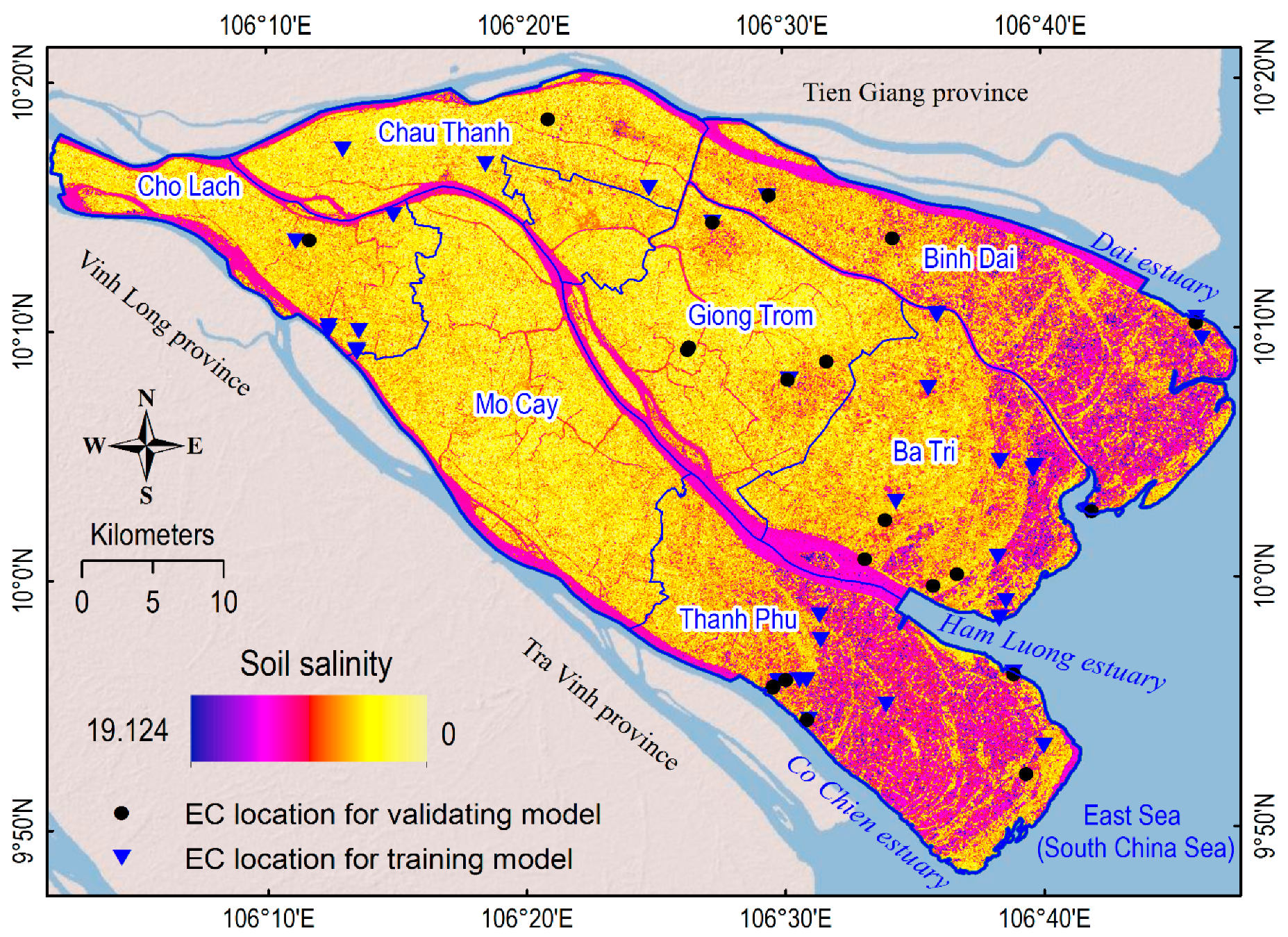
2.1. Description of the Study Area

The study area is the Ben Tre province, which is located in the Mekong river delta in the Southern Vietnam (Figure 1). It lies between longitudes 106°1′30″ and 106°47′35″, and between latitudes 9°48′26″ and 10°19′56″, covering an area of 2360.2 km². Average elevation of the province is 1–2 m above the sea level. The population of the province is 1,267,060 people in 2017 and the distribution is uneven. More than 90.3% of the population reside in rural areas where agriculture and aquaculture are the main economics sectors. Around 75.4% of the total area is the agricultural land (around 178,000 ha), which includes the rice land (45.5%), the vegetable land (3.0%), the sugar cane land (3.3%), the aquaculture land (18.0%), and other [23].

Climate patterns are characterized by a tropical monsoon with two separated seasons, a rainy season from May through November and a dry season lasting from December to April [24]. The average rainfall is from 1200 mm–1500 mm and the rainfall is mostly distributed in the rainy season (>75% the total yearly rainfall). Temperature is quite stable throughout the year with an average temperature of 27 °C. The hottest month is May where the temperature may reach to 29 °C, whereas the coolest month is December the temperature could down to 25 °C [23].

Soil in the province is characterized by high in sediments driven by the annual flood events in the low Mekong River Delta [24] and can be classified by three main types, alluvial, acid sulfate, and saline [25]. In the province, salinity intrusion is a naturally problem where the saline water intrudes the land when tide rises through the three rivers, the Dai river, the Ham Luong river, and the Co Chien river (Figure 1). In recent years, this problem, which has seriously influenced to the rice production and other agricultural activities, is seemed to be severe due to groundwater extractions, dam operations at the upstream of the Mekong river, and climate change [26]. The salinity intrusion problem is particularly severe in the dry season (January to April) due to very low discharges of the river system. Therefore, study on soil salinity and its intrusion for land-use management and finding prevention measures in this province is an urgent task in Vietnam.

2.2. Data Used

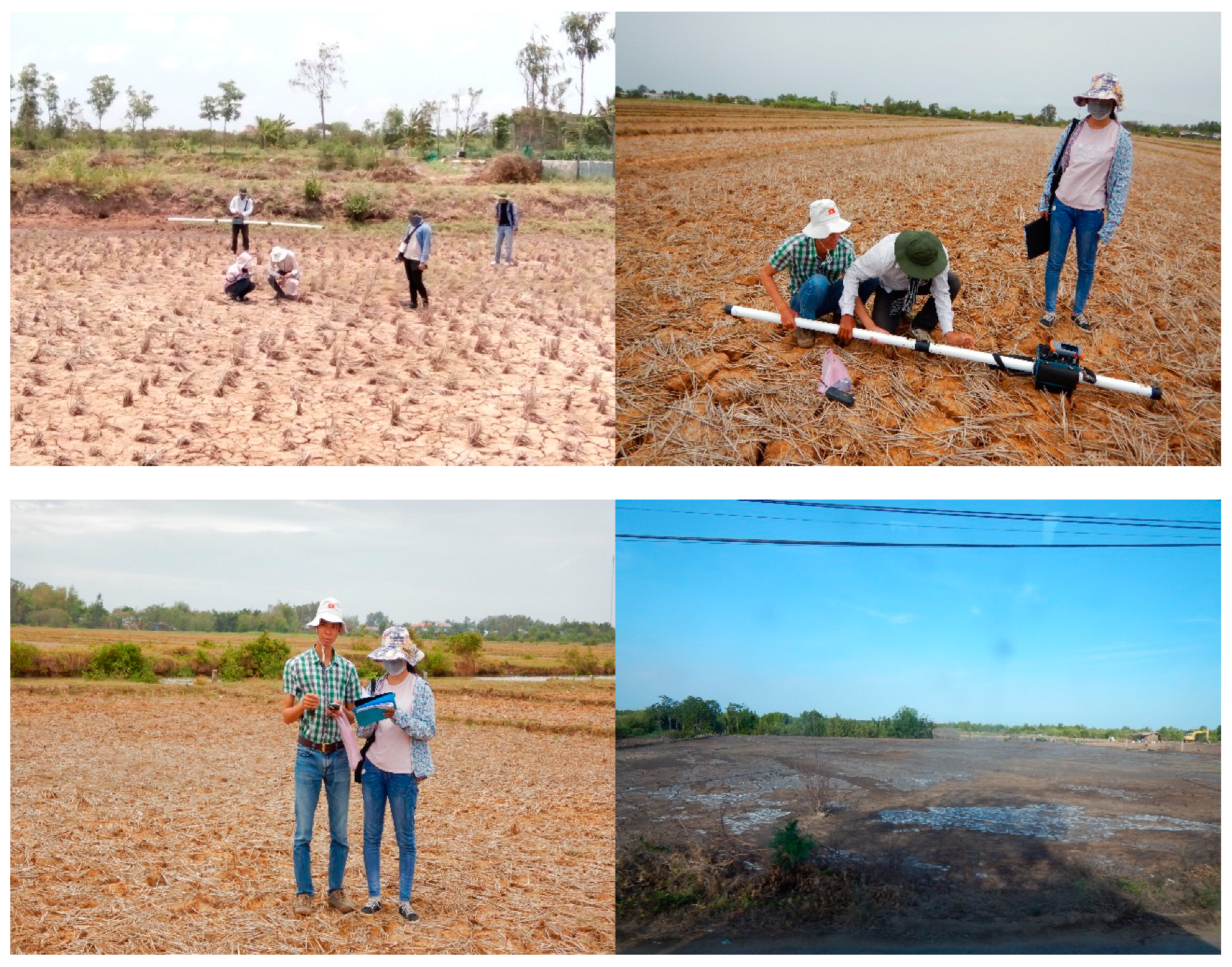
2.2.1. Soil Sample Collection and Processing

Because the salinity intrusion problem is particularly severe from January through April, especially in April every year; therefore, field surveys were carried out from 4–6 April 2018 to correspond to the Sentinel-1 SAR imagery acquired. A total of 63 sites were investigated and collected soil samples. These sites were selected by hand based on the land-use status map 1:25,000 which was provided by the local authority of the province. However, this map was produced on 2015; therefore, it was only a very coarse guidance for selecting these sites. Coordinates of the investigated sites in the national reference system (VN-2000, UTM map projection, Zone 48) were identified using a handhold GNSS (Global Navigation Satellite System). The depth of the collected soil was from 0–30 cm, and as a result, 63 soil samples were collected. Figure 2 shows photos of two sample site at the Ben Tre province.

When the collected samples arrived at the laboratory, they were kept in the enamel tray, where the temperature of the laboratory room was controlled to be not exceeding 35 °C. Subsequently, pieces of material in the samples such as stone, wood, and roots were removed before being finely ground with an agate mortar and pestle until they were passed through a 2 mm sieve. In the next step, the electrical conductivity (EC) was measured from an unfiltered 1:5 soil/deionized water suspension [27] at 25 °C. Soil suspensions were prepared using 35 mL of distilled water and 7 g of soil into 50 mL plastic centrifuge tubes (No. 06-443-20, Fisherbrand), and then, they were shaken continuously using a mechanical shaker (132 rpm) for 60 min and at 25 °C to dissolve soluble salts. Finally, EC was determined using a conductivity probe (Sension 378; Hach Co., Loveland, CO, USA). It is noted that the EC meter was calibrated by KCl standard solution (1.413 dS/m) (Cat. No. 2974326, Hach Company, Loveland, CO, USA) prior to soil suspensions measurement.

2.2.2. Sentinel-1 SAR Data

In this research, a Sentinel-1B SAR Interferometric Wide-Swath Mode (IW) image for the study area was obtained from the European Space Agency (ESA) Copernicus Sentinels Science hub (https://scihub.copernicus.eu/). In the IW, the Sentinel-1B acquires images over a 250 km swath at 5 m by 20 m spatial resolution [28]. It should be noted that the Sentinel-1 mission consists of two satellites, Sentinel-1A (launched on 3 April 2014) and Sentinel-1B (launched on 25 April 2016), which carry the C-band SAR instrument (3.75–7.5 cm wavelength and central frequency of 5.404 GHz) onboard, providing a revisit cycle of 6-day [29,30]. We selected the Sentinel-1B SAR data acquired at 6 April 2018 because it matched to the dates of the field surveys of this project. The image was acquired in the descending direction and processed to the standard Level-1 ground range detected format (10 m resolution) and in two dual-polarized, VV and VH. The incidence angle ranges from 30.85° to 45.97°.

2.3. Machine Learning Algorithms Used

Because the accuracy of soil salinity mapping is dependent on method used and no method is the best for all region [22,31]; therefore, in this research, five advanced machines learning algorithms were considered, Multilayer perceptron neural network, Radial Basis Function neural networks, Gaussian Processes, Support Vector Regression, and Random Forests. Since detailed descriptions of these algorithms are well-presented in literature i.e., in [32]; therefore, in this section, some of the main salient features of these algorithms were outlined.

2.3.1. Neural Networks

Neural Network (NN) is one of the popular machine learning algorithms and has proven its efficiency in estimating various biophysical parameters using satellite images, such as soil moisture [33], soil salinity [31], and digital soil mapping [31]. The main advantages of NN is that it is flexible and works well for complex problems with high prediction accuracy, with both large and small samples. The performance of NN is influenced by its structure and algorithms used to optimize its weights. Although many NNs have been proposed, however, for regression problems, Multilayer perceptron NN (MLP-NN) and Radial Basis Function NN (RBF-NN) are considered as the most widely used [34]; therefore, they were selected for this analysis.

For MLP-NN, this model has typically three layers, input, hidden, and output. The number of input neuron is equal to number of input variables, whereas the number of hidden neuron must be computed, whiles, the number of output neuron is one presenting the values of EC in this research. Behavior of the MLP-NN model is characterized by synoptic weights between the three layers. These weights are initiated, and then, updated using the back-propagation algorithm [35] through iteration processes.

For RBF-NN, this model also consists of three layers as in MLP-NN; however, it differs from the hidden layer carried out computations [36]. Thus, the hidden layer of RBF-NN is alluded to the RBF units, which cluster the input neurons into new space using the K-means algorithm. For build the RBF-NN model only number of cluster is required.

2.3.2. Gaussian Process

Gaussian Process regression (GP) belongs to powerful state-of-the art machine learning algorithms, which have widely used for estimating biophysical parameters using satellite imagery i.e., chlorophyll concentration [37], soil moisture [38], and forest aboveground biomass [39]. Using a Bayesian statistics, GP formulates the regression model where its parameters are assumed to follow a Gaussian distribution. The main advantage of GP is possibility to automatically optimize its parameters [40] to derive high performance models.

Consider a soil salinity dataset D = ([X_i, y_i], i = 1, 2, …, m) with X_i ∈ R_n is a matrix of m input variables with n observation, whereas y_i ∈ R is the output value, i.e., electrical conductivity (EC) in this research, the relation of the input and output variables is formulated via GP by using the equation as follow:

$$\mathsf{ŷ}=f\left(x\right)={\displaystyle \sum }_{i=1}^n{\alpha }_{i}K\left(X_i,X\right)$$

(1)

where α_i is the weight and K is the Radial Basis kernel function (RBF) (Equation (2)) [41].

$$K\left(X_i,X\right)=\beta exp\left(-{\displaystyle \sum }_{i=1}^m\frac{{\left(X_i^{\left(m\right)}-X^{\left(m\right)}\right)}^2}{2{\sigma }^2}\right)$$

(2)

where β is the scaling factor and σ is the kernel parameter.

The performance of the GP model is dependent on the parameters β and weights α_i and they could be automatically turned and optimized through maximizing the marginal likelihood [42]. Whereas, the parameters σ was determined based on the data at hand.

2.3.3. Support Vector Regression

Support vector regression (SVR) is a regression version of support vector machines, which was developed based on the statistical learning theory [43]. This is considered one of the most powerful technique advanced machine learning techniques for computing biophysical parameters from remote sensing data [44], such as, soil organic carbon [45], soil salinity [46], and biomass [47]. The advantage of using SVR is that only two parameters are needed to optimize and SVR works well with small training samples [48].

Several versions of SVR are available, i.e., Epsilon-SVR, Nu-SVR, and Sequential minimal optimization-RVR [49,50], however for soil salinity mapping in this research, Nu-SVR was selected due to the ability to derive high performance models. Thus, the process of building the SMO-SVR model is aiming to generate the following regression function

$$f\left(x\right)={{\displaystyle \sum }}_{i=1}^n\left({\lambda }_i-{\lambda }_i^{*}\right)k\left(x_i,x\right)+b$$

(3)

where ${\lambda }_i,{\lambda }_i^{*}$ denote Lagrange multipliers and $k\left(x_i,x\right)$ is the RBF kernel function.

Overall, performance of the SVReg model is controlled by three parameters C, σ, and nu; therefore, they should be carefully selected.

2.3.4. Random Forests

Random Forests (RF), which was proposed by Breiman [51], is an ensemble based algorithm where the RF model is constructed from sub-decision trees. Thus, using the training dataset D, subsets are generated using bootstrap aggregating algorithm [52], and then, each subset is used to construct a sub-decision tree using the CART (Classification And Regression Trees) algorithm. At last, a committee is formed by aggregating all sub-decision trees and the RF model is derived.

The RF is reported its efficiency various remote sensing-based applications i.e., mapping of soil properties [53], retrieving chemical properties of trees [54], and soil organic carbon [55]. Overall, RF is a fast algorithm and works well with noise variables. In addition, RF is capable to quantify the contribution of input variables to the constructed model, and thus, the relative importance of the input variables could be derived [53]. When building a RF model, two parameters must be properly determined, the number of input variables the number of sub-decision trees used for constructing these sub-decision trees.

3. Propose Methodology Used

This section describes the proposed methodological flow chart used in this project to derive the soil salinity map for the study area (Figure 3). The preprocessing of the Sentinel-1B SAR data was carried out using the ESA’s Sentinel Application Platform (SNAP) toolbox version 6.0, which is available at http://step.esa.int/main/toolboxes/snap. The rescaling and sampling data were carried out using ArcGIS 10.5 software (ESRI Inc., Redlands, CA, USA, 2018), whereas the modeling process was carried out in Matlab environment using machine learning WEKA API tool [56]. In addition, a python script, which was programmed by the authors, was used to convert the modeling result to a raster format to open in the ArcGIS software.

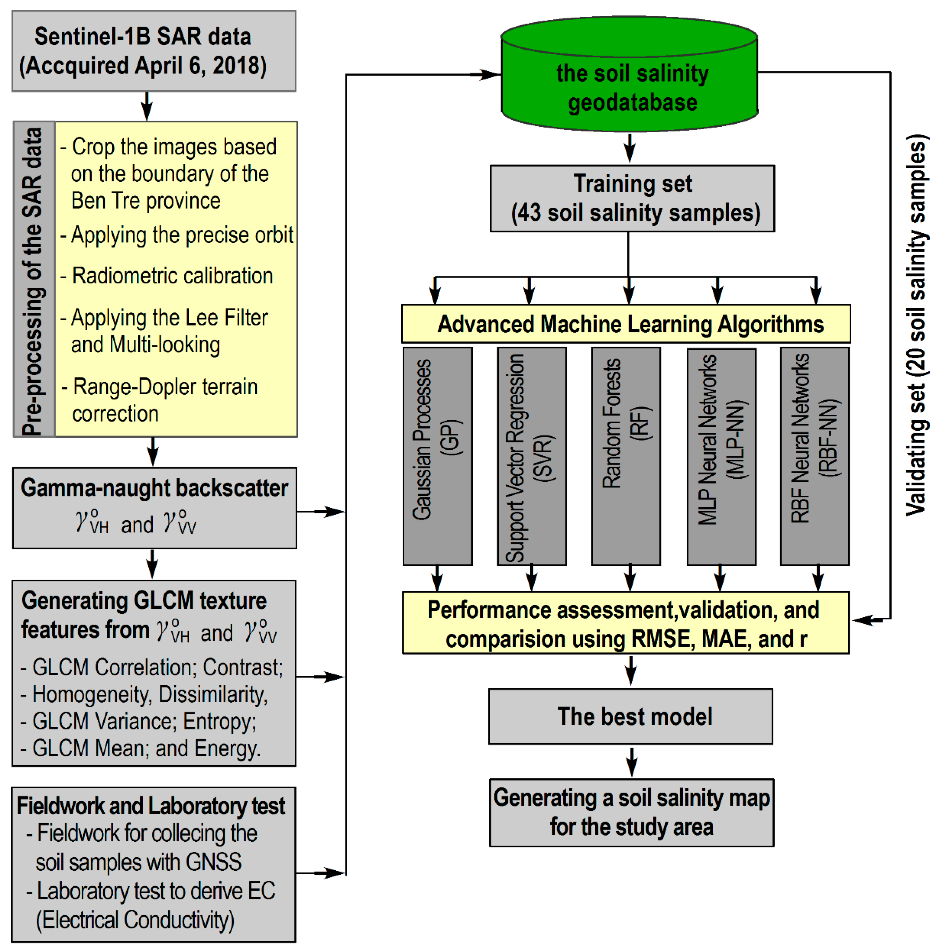
3.1. Preprocessing of the Sentinel-1 SAR Data

The pre-processing of the Sentinel-1B IW GRDH (Ground Range Detected in High resolution) data was carried out through the following steps [57]: first, application of the precise Sentinel-1B orbit, which helps to improve the geolocation accuracy, was carried out using the Sentinel Application Platform (SNAP) software [58]. Subsequently, the raw amplitude bands, VV and VH, were radiometrically calibrated to gamma-naught backscatter, ${\gamma }_{VV}^o$ and ${\gamma }_{VH}^o$. The purpose of this calibration was to derive reliable radar backscattering coefficients. It is emphasis that we used the gamma-nought in this study instead of the sigma-nought, a common backscattering coefficient used in the soil salinity mapping [22,31,59], because the gamma-nought backscattering coefficient is less sensitive to the undesirable effects of incidence angles on brightness values [60,61]. In the next step, the two calibrated ${\gamma }_{VV}^o$ and ${\gamma }_{VH}^o$ bands were filtered by applied the Median filter [62] using a 5 × 5 window [63] to reduce speckles and preserve edges [64], and then, the multi-looking process was applied. Next, the Range-Doppler geometric correction task was carried out to remove terrain induced distortions using NASA’s SRTM DEM (Shuttle Radar Topography Mission Digital Elevation Model) [65]. Finally, the resulting image bands were re-projected to the national reference system (VN-2000, UTM map projection, Zone 48) using the Bilinear resampling technique and clipped to the boundary of the study area (the Ben Tre province).

3.2. Soil Salinity Geodatabase, the Training Set, and the Validation Set

Once the image was successfully preprocessed, the final ${\gamma }_{VV}^o$ and ${\gamma }_{VH}^o$ bands were derived, and they were used as the first two input variables for the soil salinity modeling. In addition, texture features deriving from the two bands, ${\gamma }_{VV}^o$ and ${\gamma }_{VH}^o$, were considered for the soil salinity mapping. This is because textures relate to structures and physical properties of the terrain surface, which have proven their efficiency in salt-affected soil mapping [66]. To derive texture features, the Grey Level Co-occurrence Matrix (GLCM) method proposed by Haralick, et al. [67] was used. GLCM provides radar brightness values that may be considered as key information of structural characteristics of surfaces and their correlations to the neighboring environment. According to Ren, et al. [68], there is existed linear relationships between salt-affected soils and GLCM based texture features.

In this research, eight GLCM based texture features, which were extracted from the final ${\gamma }_{VV}^o$ and ${\gamma }_{VH}^o$ bands, were used for soil salinity. They are correlation texture, contrast texture, homogeneity texture, dissimilarity texture, variance texture, entropy texture, energy texture, and mean texture. The detailed formulas for computing these feature can be found in Taghadosi, Hasanlou, and Eftekhari [22]. To compute these GLCM texture features, values at ${\gamma }_{VV}^o$ and ${\gamma }_{VH}^o$ were quantized into 32 bins and a window size of 5 × 5 was used. The computation was carried out using the ESA SNAP toolbox. As a result, a total of 18 input variables (

Table 1. Importance of the input variables using the Random Forests (RF) measured by the average impurity decreased. MSE: mean squared error.

Input Variable	Permutation-Based MSE Reduction	Number of Nodes Used in the RF Model	Variable Importance Ranked
$GLCMVariance({\gamma }_{VH}^o)$	135.33	584	1
$GLCMMean({\gamma }_{VH}^o)$	133.32	677	2
${\gamma }_{VH}^o$	115.98	1089	3
$GLCMVariance({\gamma }_{VV}^o)$	81.23	314	4
$GLCMCorrelation({\gamma }_{VH}^o)$	53.39	591	5
${\gamma }_{VV}^o$	50.98	457	6
$Dissimilarity({\gamma }_{VV}^o)$	49.29	347	7
$GLCMMean({\gamma }_{VV}^o)$	47.82	351	8
$Homogeneity({\gamma }_{VH}^o)$	44.48	349	9
$Energy({\gamma }_{VH}^o)$	42.98	731	10
$GLCMCorrelation({\gamma }_{VV}^o)$	42.04	294	11
$Energy({\gamma }_{VV}^o)$	40.13	414	12
$Entropy({\gamma }_{VV}^o)$	39.70	343	13
$Entropy({\gamma }_{VH}^o)$	35.52	538	14
$Homogeneity({\gamma }_{VV}^o)$	33.08	346	15
$Contrast({\gamma }_{VV}^o)$	32.14	440	16
$Dissimilarity({\gamma }_{VH}^o)$	27.33	611	17
$Contrast({\gamma }_{VH}^o)$	27.26	736	18

), which were in a raster format with a grid size of 10 m, were prepared for soil salinity mapping in this research.

Since the soil salinity modeling using machine learning techniques required input values in the rank 0–1 [32], all input variables (maps) were normalized using Equation (4) in ArcGIS. Finally, a sampling process was carried out between the 63 soil samples and 18 input variables to build a soil salinity database.

$$Ip.norm=\frac{Ip-Ip.min}{Ip.max-Ip.min}$$

(4)

where Ip.norm is the normalized value; Ip is the actual value; Ip.max and Ip.min are the maximum value and minimum value.

In the next step, the soil salinity database was randomly separated into two subsets, the first one was a training set, which consists of 43 samples, was used to train soil salinity models, whereas the second one was a validating set (20 samples), which was used to check the prediction performance of these models and confirm their accuracy.

3.3. Feature Selection

Because 16 variables were generated from the two gamma-naught backscatter bands, ${\gamma }_{VV}^o$ and ${\gamma }_{VH}^o$; therefore, it is necessary to check if some of them may be redundant due to having similar values [22] or existed noises, which reduce performance of the resulting soil salinity models. For this task, in this research, the Random Forests algorithm (RF) was used for feature selection due to its ability to take into accounts both the impact of each variable individually and the interaction among all variables used [69]. It is noted that the RF was at first developed for classification and regression issues, but later the RF was employed for feature selection. According to Genuer, et al. [70] and Grömping [71], the RF based variable importance can be efficiently used for problems with both standard and high numbers of input variables, low numbers of samples used, and for both regression and classification.

In the RF, the bootstrap aggregating algorithm was used to generate bootstrap sets from the soil salinity training set, however, it is still around one-third of the training samples are not used [71] and they are called ‘out-of-bag’ (OOB) samples, which are used to assess the prediction performance of the RF model. Thus, the importance of an input variable can be measured by the permutation-based mean squared error (MSE) reduction [70] as follow:

Firstly, with the decision tree t, which was constructed from a bootstrap set, MSE was calculated as below:

$$MS{E}_{OOB}^t=\frac{1}{nOOB\left(t\right)}{\displaystyle \sum }_{i=1}^{nOOB}(y_i-{\mathsf{ŷ}}_{iOOB,t})$$

(5)

where $MS{E}_{OOB}$ is mean squared error; nOOB is the total OOB samples; $y_i$ is the measure EC value; and ${\mathsf{ŷ}}_{iOOB,t}$ is the predicted EC of the i-th sample from the decision tree t, in which this sample has been OOB.

Secondly, for input variable x_i, which was permuted, MSE was calculated using the following equation:

$$MS{E}_{OOB}^t\left[x_{i}permuted\right]=\frac{1}{nOOB\left(t\right)}{\displaystyle \sum }_{i=1}^{nOOB}(y_i-{\mathsf{ŷ}}_{iOOB,t}\left[x_{i}permuted\right])$$

(6)

Finally, variable importance of x_i was computed using the following equation [70]

$$\mathrm{VI}(x_i)=\frac{1}{Ttree}{{\displaystyle \sum }}_{t=1}^{Ttree}(MS{E}_{OOB}^t\left[x_{i}permuted\right]-MS{E}_{OOB}^t)$$

(7)

where Ttree is the total sub-decision trees of the RF model.

It could be seen that the difference between $MS{E}_{OOB}$ and $MS{E}_{OOB}\left[x_{i}permuted\right]$ in the entire forest model was used to assess the importance of this input variable x_i. In other words, an input variable has no predictive value for the EC when no difference between $MS{E}_{OOB}$ and $MS{E}_{OOB}\left[x_{i}permuted\right]$.

3.4. Model Configurating and Training

Using the training dataset, the five machine learning models were configured and trained. For the Gaussian Processes (GP) model, the best kernel parameter σ was determined based on a trial-and-test analysis. Thus, by varying values for the parameter σ, and then, computed three statistical metrics (RMSE, MAE, and r), σ = 1.205 is the best for the study area. For the Support Vector Regression (SVR) model, three parameters, nu, C, and gamma must be determined using the grid search method and nu = 0.579, C = 1.971, and gamma = 3.77 were the best for the soil salinity data. Regarding the Random Forests (RF) model, for this research, all input variables of the soil salinity were used for generating these sub-decision trees and 1000 sub-trees [72,73] were used to prevent the model from a problem of poor diversity. To construct the MLP-NN model for soil salinity mapping in this research, the logistic sigmoid was selected as the activation function and the linear function was used as the transfer functions, whereas the learning rate of 0.3 and the momentum of 0.2 were used, whereas the maximum iteration is 500 [73]. The best MLP-NN model with 6 hidden neuron was determined via a trial-and-test analysis presented in [45] (see result in Section 4.2). For building the RBF-NN model for the soil salinity mapping, number of cluster is determined by using the above trial-and-test analysis by varying cluster numbers versus computed r and MAE. As a result, the RBF-NN model with 20 clusters is the best for the study areas (see result in Section 4.2).

3.5. Performance Assessment

The performance of the soil salinity models is assessed and compared using three statistical metrics, RMSE (Root Mean Square Error), MAE (Mean Absolute Error), and r (correlation coefficient).

$$\mathrm{RMSE}=\sqrt{{{\displaystyle \sum }}_{i=1}^n\frac{\left({\mathsf{ŷ}}_i-y_i\right)2}{n}}$$

(8)

$$\mathrm{MAE}=\frac{1}{n}{{\displaystyle \sum }}_{i=1}^n\left|{\mathsf{ŷ}}_i-y_i\right|$$

(9)

$$r=\frac{{{\displaystyle \sum }}_{i=1}^n\left(y_i-\overline{y}\right)\left({\mathsf{ŷ}}_i-\overline{\mathsf{ŷ}}\right)}{\sqrt{{{\displaystyle \sum }}_{i=1}^n{\left(y_i-\overline{y}\right)}^2{\left({\mathsf{ŷ}}_i-\overline{\mathsf{ŷ}}\right)}^2}}$$

(10)

where $\widehat{\mathrm{y}}$_i and y_i are the computed and measured EC values the i-th sample, respectively; $\overline{\mathrm{y}}$ and $\overline{\widehat{\mathrm{y}}}$ are the mean values of the measured EC values and the predicted EC values; and n is the total number of sample used.

3.6. Final Trained Model and Generating Soil Salinity Maps

Once the five soil salinity models were successfully trained, they were validated and compared using the validation set to determine the best model for the study area. The best model was then used to compute soil salinity values for all pixels of the study area. The result was finally exported to a raster format and open in ArcGIS 10.5 software.

4. Results

4.1. Variable Importance Assessment

Variable importance of the 18 input variables in this research was measured using the average MSE impurity reduction as described in Section 3.3 and the result was shown in Table 1. It could be seen that $GLCMVariance({\gamma }_{VH}^o)$ has the highest permutation-based MSE reduction value (135.33) indicating that it is the most important variable for the study area. It is followed by $GLCMMean({\gamma }_{VH}^o)$ (133.32), ${\gamma }_{VH}^o$ (115.98),$GLCMVariance({\gamma }_{VV}^o)$(81.23), $GLCMCorrelation({\gamma }_{VH}^o)$ (53.39), and ${\gamma }_{VV}^o$ (50.98). In contrast, $Dissimilarity({\gamma }_{VH}^o)$ (27.33) and $Contrast({\gamma }_{VH}^o)$ (27.26) have the smallest permutation-based MSE reduction values, indicating that they are the lowest important variables to the soil salinity in this research. Overall, all input variables had a certain predictive value to the soil salinity (EC); therefore, all of them were selected for developing soil salinity models for this study area.

4.2. Model Training and Their Performances

The result of the trial-and-test analysis to determine the best network structure for the MLP-NN model is shown in

Table 2. Performance of multilayer perceptron NN (MLP-NN) versus its hidden neurons (IN: Input neuron; HN: Hidden neuron; OP: Output).

No	MLP-NN (IN × HN × OP)	Training Set			Validating Set
		RMSE	MAE	r	RMSE	MAE	r
1	18 × 1 × 1	3.925	2.998	0.848	4.226	3.077	0.523
2	18 × 2 × 1	3.919	2.994	0.848	4.214	3.074	0.525
3	18 × 3 × 1	3.923	3.008	0.847	4.207	3.068	0.526
4	18 × 4 × 1	3.704	2.864	0.845	3.846	2.929	0.553
5	18 × 5 × 1	3.724	2.893	0.841	3.792	2.892	0.56
6	18 × 6 × 1	3.744	2.936	0.839	3.450	2.646	0.624
7	18 × 7 × 1	3.775	2.969	0.838	3.484	2.687	0.620
8	18 × 8 × 1	4.246	3.457	0.831	4.103	3.45	0.354
9	18 × 9 × 1	3.910	3.002	0.846	4.147	3.036	0.532
10	18 × 10 × 1	4.567	3.736	0.834	4.286	3.372	0.513
11	18 × 11 × 1	4.563	3.699	0.837	4.332	3.363	0.504
12	18 × 12 × 1	4.413	3.840	0.818	4.030	3.579	0.558
13	18 × 14 × 1	4.637	3.821	0.829	4.354	3.439	0.507
14	18 × 16 × 1	4.030	3.219	0.836	3.891	3.162	0.562
15	18 × 18 × 1	4.618	3.825	0.833	4.388	3.561	0.481
16	18 × 20 × 1	4.581	3.823	0.830	4.327	3.620	0.479
17	18 × 22 × 1	2.413	1.829	0.904	4.643	3.615	0.320
18	18 × 24 × 1	2.206	1.519	0.913	4.427	3.079	0.565
19	18 × 26 × 1	2.251	1.592	0.912	4.079	3.019	0.558
20	18 × 28 × 1	2.512	1.878	0.901	4.423	3.052	0.542
21	18 × 30 × 1	2.211	1.523	0.912	4.070	2.862	0.551

, where the number of hidden neurons was varied from 1 to 30, and then, RMSE, MAE, and r were estimated on both the training set and the validation set. Overall, the degree-of-fit of the MLP-NN model with the training set raised when the number of the hidden neurons was increased. However, the prediction performance the MLP-NN model increased from the structure 18 × 1 × 1 (RMSE = 4.226, MAE = 3.077, and r = 0.523) to the structure 18 × 6 × 1 (RMSE = 3.450, MAE = 2.646, and r = 0.624), and then, the prediction performance was decreased with the increasing hidden neurons; therefore, the best structure of the MLP-NN model was 18 × 6 × 1 (

Table 3. Performance of RBF-NN versus its clusters (IN: Input neuron; CL: Number of clusters; OP: Output).

No	RBF-NN (IN × CL × OP)	Training Set			Validating Set
		RMSE	MAE	r	RMSE	MAE	r
1	18 × 2 × 1	5.302	3.247	0.005	4.136	3.022	0.121
2	18 × 3 × 1	5.247	3.068	0.144	4.211	3.096	−0.051
3	18 × 4 × 1	5.160	2.962	0.230	4.308	3.134	0.006
4	18 × 5 × 1	5.043	2.829	0.309	3.747	2.608	0.431
5	18 × 6 × 1	4.649	2.691	0.481	5.011	3.309	−0.226
6	18 × 7 × 1	4.663	2.741	0.476	4.730	3.012	−0.115
7	18 × 8 × 1	4.663	2.736	0.476	4.823	3.223	−0.114
8	18 × 9 × 1	4.640	2.744	0.484	4.339	3.092	0.187
9	18 × 10 × 1	4.680	2.684	0.470	4.112	2.832	0.291
10	18 × 11 × 1	4.554	2.517	0.512	4.324	2.836	0.218
11	18 × 12 × 1	4.299	2.539	0.585	4.103	2.855	0.301
12	18 × 14 × 1	4.217	2.452	0.606	4.775	3.123	0.045
13	18 × 16 × 1	4.402	2.414	0.557	4.556	3.052	0.178
14	18 × 17 × 1	3.833	2.096	0.691	2.981	1.924	0.729
14	18 × 18 × 1	3.833	2.087	0.691	3.210	2.074	0.692
15	18 × 19 × 1	3.825	2.08	0.693	3.187	2.008	0.707
16	18 × 20 × 1	3.760	1.934	0.705	3.249	2.059	0.698
17	18 × 21 × 1	3.702	1.822	0.716	2.732	1.586	0.772
18	18 × 22 × 1	3.510	1.655	0.750	7.225	3.417	0.327
19	18 × 24 × 1	3.508	1.612	0.750	7.142	3.362	0.323
20	18 × 26 × 1	3.344	1.492	0.776	7.130	3.382	0.191
21	18 × 28 × 1	3.370	1.489	0.772	7.353	3.593	0.118
22	18 × 30 × 1	3.330	1.364	0.778	7.558	3.746	0.072

).

Regarding the RBF-NN model, the same procedure, which was used for the MLP-NN model, was employed to determine the best number of clusters for the network structure. In general, the degree-of-fit of the RBF-NN model with the training set increased when we increased the cluster numbers. However, with the validation set, the prediction performance increased from the RBF-NN model with 2 clusters (RMSE = 4.136, MAE = 3.022, and r = 0.121) to the RBF-NN model with 21 clusters, and then, the prediction performance was deceased with the increasing the cluster number (Table 3); therefore, the best structure of the RBF-NN model was 18 × 21 × 1 (RMSE = 2.732, MAE = 1.586, and r = 0.772).

Regarding the other three models, as indicated in Section 3.4, σ = 1.205 was the best for the GP model with the soil salinity data, whereas with the SVR model, nu = 0.579, C = 1.971, and gamma = 3.77 were the most suitable and for the RF model, 500 trees were used.

The final training and validating results of the five soil salinity models were shown in

Table 4. Performance of the five soil salinity models using both the training set and the validation set in this research. RMSE: root mean squared error.

Soil Salinity Model	Training Set			Validation Set
	RMSE	MAE	r	RMSE	MAE	r
Multilayer Perceptron Neural Networks (MLP-NN)	3.744	2.936	0.836	3.450	2.646	0.624
Radial Basis Function Neural Networks (RBF-NN)	3.702	1.822	0.716	2.732	1.586	0.772
Gaussian Processes (GP)	3.170	1.860	0.839	2.885	1.897	0.808
Support Vector Regression (SVR)	4.784	1.868	0.685	3.946	2.091	0.664
Random Forests (RF)	2.008	1.252	0.949	3.417	2.269	0.581

and Figure 4 and Figure 5. It could be seen that only four models (RF, GP, RBF-NN) had satisfactory goodness-of-fit to the training set. The highest fit was found for the RF model (RMSE = 2.008, MAE = 1.252, and r = 0.949), followed by the GP model (RMSE = 3.170, MAE = 1.860, and r = 0.839), the MLP-NN model (RMSE = 3.744, MAE = 2.936, and r = 0.836), and the RBF-NN model (RMSE = 3.702, MAE = 1.822, and r = 0.716). In contrast to these models, the SVR model had a low fit to the training set (RMSE = 4.784, MAE = 1.868, and r = 0.685).

Regarding the validating result, the GP model had the highest prediction performance (RMSE = 2.885, MAE = 1.897, and r = 0.808), followed by the RBF-NN model (RMSE = 2.732, MAE = 1.586, and r = 0.772). The other three models, the SVR model (RMSE = 3.946, MAE = 2.091, and r = 0.664), the MLP-NN model (RMSE = 3.450, MAE = 2.646, and r = 0.624), and the RF model (RMSE = 3.417, MAE = 2.269, and r = 0.581), had somewhat low prediction performance.

4.3. Soil Salinity Map

Based on the above analysis, it could be concluded that the GP model is the best for soil salinity mapping of the study area; therefore, the GP model was used to compute soil salinity value for each of all pixels of the Ben Tre province, and then, a soil salinity was generated (Figure 6). Aerial interpretation of the map shows that areas at three districts, Thanh Phu, Ba Tri, and Binh Dai have high degrees of salinity. This is because the three districts are near the East Sea (South China Sea) where the saline water intrudes the land when tide rises through the Dai river, the Ham Luong river, and the Co Chien river. In contrast, areas at the Cho Lach district, the Chau Thanh district, and the Mo Cay district have lower salinity values due to the geographic positions, which are far from the East Sea.

5. Discussion

Soil salinization is still a serious problem worldwide, which affects the natural environment, causes losses of agricultural productivity, and food safety [74]; therefore, soil salinity mapping is important, providing useful information of soil salinity level, which may be useful for land-use planning and management [75]. This study addressed the above issue through evaluating the potential of Sentinel-1 SAR imagery for estimating soil salinity using the five state-of-the-art machine learning algorithms. The key issue of using radar images in the soil salinity mapping in this research is that soil moisture content and salinity relating to the soil dielectric properties which are sensitive with radar signals [12]. Also, for soils with dark colored surface layers and over coastal areas where the soil surface is highly affected by moisture content, optical remote sensing imagery provides inaccurate results [38].

It should be noted that due to lack of a suitable scattering model for modeling SAR backscatter of soil based on salt content, fewer studies have been done in radar remote sensing for salinity estimating, and most of related studies have been dedicated in investigating the spectral behavior of salt affected soils in the visible range of the electromagnetic spectrum. However, determining and assessing the contingency of using Sentinel-1 imagery to map soil salinity and create a relationship between EC measuring and Sentinel-1 data have importance, supporting to cover the weakness of the proposed modeling in this field. Therefore, attention in this paper is to investigate the relationship between measured salinity (EC) and radar images, provided by the Sentinel-1 SAR satellite.

In this regard, due to less sensitivity of incidence angles on brightness values, the gamma-nought of two polarizations, VV and VH, were used as backscattering coefficients and as input data. By using two gamma-nought images, eighteen image-based texture features were generated and used as input variables of the five machine learning algorithms, MLP-NN, RBF-NN, GP, SVR, and RF. Also, as part of this study, to evaluate the value and rank of each feature, the RF feature selection method was used. Evaluating the performed analysis and the predicted EC results, we can observe the following results:

• Overall, it is still difficult to establish accurately relationships between the soil salinity and radar signals though several attempts have been carried out [22]. The result in this research showed that the direct correlation of each of the radar bands (${\gamma }_{VV}^o$ and ${\gamma }_{VH}^o$) to the soil salinity is low indicating that empirical model of soil salinity using single radar is not feasible and this finding is in agreement with Jiang, Rusuli, Amuti, and He [31]. Therefore, combination of various factors is suggested to derive more accuracy models. As a result, 16 texture features derived from the two bands, ${\gamma }_{VV}^o$ and ${\gamma }_{VH}^o$ were considered.
• Feature selection was carried out for the 18 input features using RF and the permutation-based MSE reduction value of them varies from 27.26 to 135.33. This indicates that the 18 input features offer certain predictive values to the soil salinity. Further tests were carried out by removing features with low permutation-based MSE reduction values, and then, checking if with the reducing the feature set, the performance of the five regression models may be improved; however, no performance improvement was found. Therefore, it could be concluded that all the incorporated features used for modeling are appropriate and suitable for soil salinity modeling with machine learning methods.
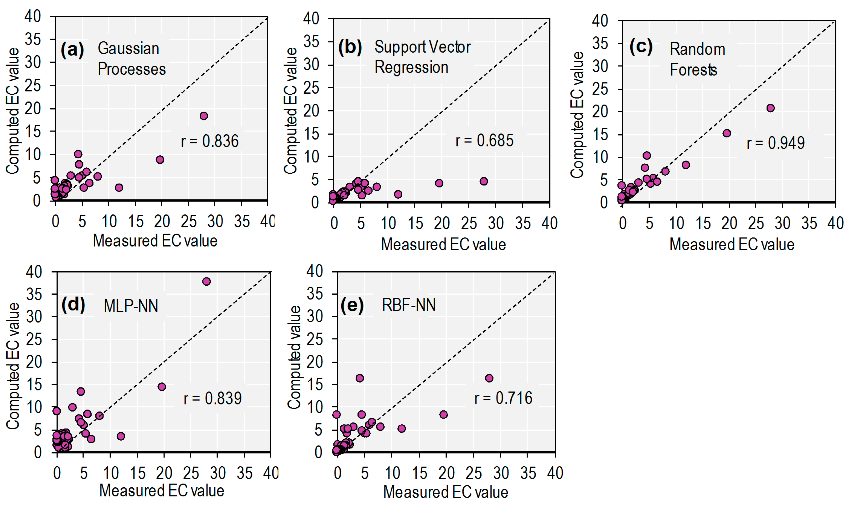
• Performance of the five regression models (the MLP-NN, the RBF-NN, the GP, the SVR, and the RF) used in this study continues confirming that soil salinity mapping is dependent on methods and techniques used [22,31]. Among the five models, the GP with RBF kernel function shows the most accuracy (r = 0.808, RMSE = 2.885, and MAE = 1.897). Although the RBF-NN model has lower MAE (1.586) and RMSE (2.732) compared to the GP model; however, correlation coefficient (r = 0.772) of the RBF-NN model is clear lower than that of the GP model. Therefore, GP is a powerful tool, which should be used for soil salinity mapping. The other three models (the MLP-NN, the SVR, and the RF) provide poorly prediction performance though they fit quit well with the training data, indicating that these models exist some degrees of over-fitting. This is because this research has a relatively small number of samples. In addition, both the training and validating set exist samples with extremely high EC values, which are difficult for these models to learn and predict.
• Evaluation of the predicted salinity values, which were obtained from the MLP-NN and the RBF-NN, reveals that the RBF-NN model has better prediction performance comparing to the MLP-NN. In RBF-NN model, the best setting achieved by using 18 as input neuron and 21 as number of clusters. In other side, the MLP-NN reach to EC map by incorporating 18 as input neuron and 6 as hidden neurons with the r = 0.624 and the lowest RMSE of 3.450 (when using all features). Nevertheless, both MLP-NN and RBF-NN provided poorly accuracy results in this research; therefore, newer neural network structures i.e., deep learning neural networks should be investigated.
• For the SVR model, this model had difficulties in learning with extremely high values of EC (three samples with EC values >12 in the training set). In other words, these samples caused a low degree-of-fit of the model. Consequently, the SVR model lacks sensitivities to samples with high EC values in the validating set. More specifically, three samples with EC values >7.9 were predicted as being below 4. In addition, the performance of the SVR model is influenced by its three parameters (C, σ, and nu) and although the grid search algorithm was used to determine the best values for the three parameters; however, it is difficult to conclude that these are the optimal values. Therefore, new machine learning optimization algorithms should be considered to find the optimized values for the three parameters.
• Regarding the RF model, although this model showed excellent goodness-of-fit, but it provided lowest prediction result. This is due to the natural limitation of this algorithm which usually predicted poor results then values in the validating set are outside those in the training sets that the RF was used to trained [76].
• Overall, the result in this research shows that the incorporating machine learning methods and the Sentinel-1 radar imagery for produce soil EC map with good accuracy is viable. Now, it is possible to estimate salinity for each 10 m × 10 m area at very short intervals of about 6 days. This represents the Radar remotely sensed data as a useful tool for land management studies and soil reclamation programs.

6. Conclusions

This research has evaluated the potential of Sentinel-1 SAR imagery and the five state-of-the-art machine learning algorithms (the MLP-NN, the RBF-NN, the GP, the SVR, and the RF) to map soil salinity intrusion in the Ben Tre province located on the Mekong River Delta of Vietnam. Based on the obtained results, the following conclusions are derived:

• Although the optical remote sensing images, i.e., Landsat 8 OLI and Sentinel-2 have proven their efficiency in the soil salinity mapping on other areas; however, they are not suitable for the tropical province of Ben Tre due to cloud cover problems.
• Sentinel-1 SAR data, which are not affected by weather conditions, have enough capability to separate saline soils directly by using machine learning methods. It can be concluded that it is conceivable to map soil salinity at short intervals of about 6 days for each 10 m × 10 m area, using the potential of the Sentinel-1 satellite image data and the GP method. This confirms remote sensing as a powerful technology for salinity mapping.
• Texture features derived from the two bands, ${\gamma }_{VV}^o$ and ${\gamma }_{VH}^o$ and Random Forest with Permutation-based MSE reduction are useful for soil salinity modeling.
• Incorporating the potential of full polarized SAR images in different frequency bands (P, L, C, and X) and applying various target decomposition methods to SAR image data for generating salinity models is recommended for future studies.

References

1. Metternicht, G.; Zinck, A. Remote Sensing of Soil Salinization: Impact on Land Management; CRC Press: Boca Raton, FL, USA, 2008. [Google Scholar]
2. Metternicht, G.I.; Zinck, J.A. Remote sensing of soil salinity: Potentials and constraints. Remote Sens. Environ. 2003, 85, 1–20. [Google Scholar] [CrossRef]
3. FAO. FAO Soils Portal. 2016. Available online: http://www.fao.org/soils-portal/soil-management/management-of-some-problem-soils/salt-affected-soils/more-information-on-salt-affected-soils/en/ (accessed on 15 November 2018 ).
4. Allbed, A.; Kumar, L.; Sinha, P. Mapping and Modelling Spatial Variation in Soil Salinity in the Al Hassa Oasis Based on Remote Sensing Indicators and Regression Techniques. Remote Sens. 2014, 6, 1137–1157. [Google Scholar] [CrossRef] [Green Version]
5. Allbed, A.; Kumar, L.; Aldakheel, Y.Y. Assessing soil salinity using soil salinity and vegetation indices derived from IKONOS high-spatial resolution imageries: Applications in a date palm dominated region. Geoderma 2014, 230–231, 1–8. [Google Scholar] [CrossRef]
6. Douaoui, A.E.K.; Nicolas, H.; Walter, C. Detecting salinity hazards within a semiarid context by means of combining soil and remote-sensing data. Geoderma 2006, 134, 217–230. [Google Scholar] [CrossRef]
7. Sidike, A.; Zhao, S.; Wen, Y. Estimating soil salinity in Pingluo County of China using QuickBird data and soil reflectance spectra. Int. J. Appl. Earth Obs. Geoinf. 2014, 26, 156–175. [Google Scholar] [CrossRef]
8. El Harti, A.; Lhissou, R.; Chokmani, K.; Ouzemou, J.-E.; Hassouna, M.; Bachaoui, E.M.; El Ghmari, A. Spatiotemporal monitoring of soil salinization in irrigated Tadla Plain (Morocco) using satellite spectral indices. Int. J. Appl. Earth Obs. Geoinf. 2016, 50, 64–73. [Google Scholar] [CrossRef]
9. Mashimbye, Z.E.; Cho, M.A.; Nell, J.P.; De Clercq, W.P.; Van Niekerk, A.; Turner, D.P. Model-Based Integrated Methods for Quantitative Estimation of Soil Salinity from Hyperspectral Remote Sensing Data: A Case Study of Selected South African Soils. Pedosphere 2012, 22, 640–649. [Google Scholar] [CrossRef]
10. Weng, Y.-L.; Gong, P.; Zhu, Z.-L. A Spectral Index for Estimating Soil Salinity in the Yellow River Delta Region of China Using EO-1 Hyperion Data. Pedosphere 2010, 20, 378–388. [Google Scholar] [CrossRef]
11. Lu, D. The potential and challenge of remote sensing-based biomass estimation. Int. J. Remote Sens. 2006, 27, 1297–1328. [Google Scholar] [CrossRef]
12. Barbouchi, M.; Abdelfattah, R.; Chokmani, K.; Aissa, N.B.; Lhissou, R.; El Harti, A. Soil salinity characterization using polarimetric InSAR coherence: Case studies in Tunisia and Morocco. IEEE J. Sel. Top. Appl. Earth Obs. Remote Sens. 2015, 8, 3823–3832. [Google Scholar] [CrossRef]
13. Shao, Y.; Hu, Q.; Guo, H.; Lu, Y.; Dong, Q.; Han, C. Effect of dielectric properties of moist salinized soils on backscattering coefficients extracted from RADARSAT image. IEEE Trans. Geosci. Remote Sens. 2003, 41, 1879–1888. [Google Scholar] [CrossRef]
14. Engman, E.T. Applications of microwave remote sensing of soil moisture for water resources and agriculture. Remote Sens. Environ. 1991, 35, 213–226. [Google Scholar] [CrossRef]
15. Horikoshi, S.; Schiffmann, R.F.; Fukushima, J.; Serpone, N. Microwave Chemical and Materials Processing; Springer: Berlin, Germany, 2018. [Google Scholar]
16. Lasne, Y.; Paillou, P.; Freeman, A.; Farr, T.; McDonald, K.C.; Ruffie, G.; Malezieux, J.-M.; Chapman, B.; Demontoux, F. Effect of salinity on the dielectric properties of geological materials: Implication for soil moisture detection by means of radar remote sensing. IEEE Trans. Geosci. Remote Sens. 2008, 46, 1674–1688. [Google Scholar] [CrossRef]
17. Bell, D.; Menges, C.; Bartolo, R.; Ahmad, W.; VanZyl, J. A multistaged approach to mapping soil salinity in a tropical coastal environment using airborne SAR and Landsat TM data. In Proceedings of the IEEE 2001 International Geoscience and Remote Sensing Symposium, IGARSS’01, Sydney, NSW, Australia, 9–13 July 2001; IEEE: Piscataway, NJ, USA, 2001; pp. 1309–1311. [Google Scholar]
18. Metternicht, G. Fuzzy classification of JERS-1 SAR data: An evaluation of its performance for soil salinity mapping. Ecol. Model. 1998, 111, 61–74. [Google Scholar] [CrossRef]
19. Farifteh, J.; Van der Meer, F.; Atzberger, C.; Carranza, E.J.M. Quantitative analysis of salt-affected soil reflectance spectra: A comparison of two adaptive methods (PLSR and ANN). Remote Sens. Environ. 2007, 110, 59–78. [Google Scholar] [CrossRef]
20. Nurmemet, I.; Ghulam, A.; Tiyip, T.; Elkadiri, R.; Ding, J.-L.; Maimaitiyiming, M.; Abliz, A.; Sawut, M.; Zhang, F.; Abliz, A. Monitoring soil salinization in Keriya River Basin, Northwestern China using passive reflective and active microwave remote sensing data. Remote Sens. 2015, 7, 8803–8829. [Google Scholar] [CrossRef]
21. Nurmemet, I.; Sagan, V.; Ding, J.-L.; Halik, Ü.; Abliz, A.; Yakup, Z. A WFS-SVM Model for Soil Salinity Mapping in Keriya Oasis, Northwestern China Using Polarimetric Decomposition and Fully PolSAR Data. Remote Sens. 2018, 10, 598. [Google Scholar] [CrossRef]
22. Taghadosi, M.M.; Hasanlou, M.; Eftekhari, K. Soil salinity mapping using dual-polarized SAR Sentinel-1 imagery. Int. J. Remote Sens. 2018, 1–16. [Google Scholar] [CrossRef]
23. Le, A.; Du, L.; Tristan, S. Rapid integrated and ecosystem-based assessment of climate change vulnerability and adaptation for Ben Tre Province, Viet Nam. J. Sci. Technol. 2014, 52, 287–293. [Google Scholar]
24. Kontgis, C.; Schneider, A.; Ozdogan, M. Mapping rice paddy extent and intensification in the Vietnamese Mekong River Delta with dense time stacks of Landsat data. Remote Sens. Environ. 2015, 169, 255–269. [Google Scholar] [CrossRef]
25. Vo, T.B.T.; Wassmann, R.; Tirol-Padre, A.; Cao, V.P.; MacDonald, B.; Espaldon, M.V.O.; Sander, B.O. Methane emission from rice cultivation in different agro-ecological zones of the Mekong river delta: Seasonal patterns and emission factors for baseline water management. Soil Sci. Plant Nutr. 2018, 64, 47–58. [Google Scholar] [CrossRef]
26. Renaud, F.G.; Le, T.T.H.; Lindener, C.; Guong, V.T.; Sebesvari, Z. Resilience and shifts in agro-ecosystems facing increasing sea-level rise and salinity intrusion in Ben Tre Province, Mekong Delta. Clim. Chang. 2015, 133, 69–84. [Google Scholar] [CrossRef]
27. Sharma, R.; Bell, R.; Wong, M. Dissolved reactive phosphorus played a limited role in phosphorus transport via runoff, throughflow and leaching on contrasting cropping soils from southwest Australia. Sci. Total Environ. 2017, 577, 33–44. [Google Scholar] [CrossRef] [PubMed]
28. ESA. SENTINEL-1 SAR User Guide Introduction. 2016. Available online: https://sentinel.esa.int/web/sentinel/user-guides/sentinel-1-sar (accessed on 14 October 2018).
29. Rucci, A.; Ferretti, A.; Guarnieri, A.M.; Rocca, F. Sentinel 1 SAR interferometry applications: The outlook for sub millimeter measurements. Remote Sens. Environ. 2012, 120, 156–163. [Google Scholar] [CrossRef]
30. Peter, H.; Jäggi, A.; Fernández, J.; Escobar, D.; Ayuga, F.; Arnold, D.; Wermuth, M.; Hackel, S.; Otten, M.; Simons, W.; et al. Sentinel-1A—First precise orbit determination results. Adv. Space Res. 2017, 60, 879–892. [Google Scholar] [CrossRef]
31. Jiang, H.; Rusuli, Y.; Amuti, T.; He, Q. Quantitative assessment of soil salinity using multi-source remote sensing data based on the support vector machine and artificial neural network. Int. J. Remote Sens. 2018, 1–23. [Google Scholar] [CrossRef]
32. Bishop, C.M. Pattern Recognition and Machine Learning; Information Science and Statistics; Springer. Inc.: Secaucus, NJ, USA, 2006. [Google Scholar]
33. Rodríguez-Fernández, N.J.; Aires, F.; Richaume, P.; Kerr, Y.H.; Prigent, C.; Kolassa, J.; Cabot, F.; Jiménez, C.; Mahmoodi, A.; Drusch, M. Soil moisture retrieval using neural networks: Application to SMOS. IEEE Trans. Geosci. Remote Sens. 2015, 53, 5991–6007. [Google Scholar] [CrossRef]
34. Tien Bui, D.; Tuan, T.A.; Klempe, H.; Pradhan, B.; Revhaug, I. Spatial prediction models for shallow landslide hazards: A comparative assessment of the efficacy of support vector machines, artificial neural networks, kernel logistic regression, and logistic model tree. Landslides 2016, 13, 361–378. [Google Scholar] [CrossRef]
35. Haykin, S. Neural Networks: A Comprehensive Foundation, 2nd ed.; Prentice Hall: Upper Saddle River, NJ, USA, 1998; 842p. [Google Scholar]
36. Witten, I.H.; Frank, E.; Mark, A.H. Data Mining: Practical Machine Learning Tools and Techniques, 3rd ed.; Morgan Kaufmann: Burlington, VT, USA, 2011; 558p. [Google Scholar]
37. Blix, K.; Camps-Valls, G.; Jenssen, R. Gaussian process sensitivity analysis for oceanic chlorophyll estimation. IEEE J. Sel. Top. Appl. Earth Obs. Remote Sens. 2017, 10, 1265–1277. [Google Scholar] [CrossRef]
38. Stamenkovic, J.; Guerriero, L.; Ferrazzoli, P.; Notarnicola, C.; Greifeneder, F.; Thiran, J.-P. Soil Moisture Estimation by SAR in Alpine Fields Using Gaussian Process Regressor Trained by Model Simulations. IEEE Trans. Geosci. Remote Sens. 2017, 55, 4899–4912. [Google Scholar] [CrossRef]
39. Vafaei, S.; Soosani, J.; Adeli, K.; Fadaei, H.; Naghavi, H.; Pham, T.D.; Tien Bui, D. Improving accuracy estimation of forest aboveground biomass based on incorporation of ALOS-2 PALSAR-2 and sentinel-2A imagery and machine learning: A case study of the Hyrcanian forest area (Iran). Remote Sens. 2018, 10, 172. [Google Scholar] [CrossRef]
40. Rasmussen, C.E. Gaussian processes in machine learning. In Advanced Lectures on Machine Learning; Springer: Berlin, Germany, 2004; pp. 63–71. [Google Scholar]
41. Campos-Taberner, M.; García-Haro, F.J.; Camps-Valls, G.; Grau-Muedra, G.; Nutini, F.; Crema, A.; Boschetti, M. Multitemporal and multiresolution leaf area index retrieval for operational local rice crop monitoring. Remote Sens. Environ. 2016, 187, 102–118. [Google Scholar] [CrossRef]
42. Rasmussen, C.E.; Williams, C.K. Gaussian Processes for Machine Learning; MIT Press: Cambridge, MA, USA, 2006; Volume 1. [Google Scholar]
43. Vapnik, V.N. Statistical Learning Theory; Wiley-Interscience: Hoboken, NJ, USA, 1998; 736p. [Google Scholar]
44. Ali, I.; Greifeneder, F.; Stamenkovic, J.; Neumann, M.; Notarnicola, C. Review of machine learning approaches for biomass and soil moisture retrievals from remote sensing data. Remote Sens. 2015, 7, 16398–16421. [Google Scholar] [CrossRef]
45. Were, K.; Bui, D.T.; Dick, Ø.B.; Singh, B.R. A comparative assessment of support vector regression, artificial neural networks, and random forests for predicting and mapping soil organic carbon stocks across an Afromontane landscape. Ecol. Indic. 2015, 52, 394–403. [Google Scholar] [CrossRef]
46. Aldabaa, A.A.A.; Weindorf, D.C.; Chakraborty, S.; Sharma, A.; Li, B. Combination of proximal and remote sensing methods for rapid soil salinity quantification. Geoderma 2015, 239–240, 34–46. [Google Scholar] [CrossRef]
47. Garcia, M.; Saatchi, S.; Casas, A.; Koltunov, A.; Ustin, S.; Ramirez, C.; Garcia-Gutierrez, J.; Balzter, H. Quantifying biomass consumption and carbon release from the California Rim fire by integrating airborne LiDAR and Landsat OLI data. J. Geophys. Res. Biogeosci. 2017, 122, 340–353. [Google Scholar] [CrossRef] [Green Version]
48. Zhu, K.; Song, X.; Xue, D. A roller bearing fault diagnosis method based on hierarchical entropy and support vector machine with particle swarm optimization algorithm. Measurement 2014, 47, 669–675. [Google Scholar] [CrossRef]
49. Chang, C.-C.; Lin, C.-J. Training v-support vector regression: Theory and algorithms. Neural Comput. 2002, 14, 1959–1977. [Google Scholar] [CrossRef]
50. Platt, J. Sequential Minimal Optimization: A Fast Algorithm for Training Support Vector Machines. 1998. Available online: https://www.microsoft.com/en-us/research/publication/sequential-minimal-optimization-a-fast-algorithm-for-training-support-vector-machines/ (accessed on 10 January 2019).
51. Breiman, L. Random forests. Mach. Learn. 2001, 45, 5–32. [Google Scholar] [CrossRef]
52. Friedman, J.; Hastie, T.; Tibshirani, R. The Elements of Statistical Learning; Springer Series in Statistics; Springer: New York, NY, USA, 2001; Volume 1. [Google Scholar]
53. Forkuor, G.; Hounkpatin, O.K.; Welp, G.; Thiel, M. High resolution mapping of soil properties using remote sensing variables in South-Western Burkina Faso: A comparison of machine learning and multiple linear regression models. PLoS ONE 2017, 12, e0170478. [Google Scholar] [CrossRef]
54. Ferreira, M.P.; Féret, J.-B.; Grau, E.; Gastellu-Etchegorry, J.-P.; Shimabukuro, Y.E.; de Souza Filho, C.R. Retrieving structural and chemical properties of individual tree crowns in a highly diverse tropical forest with 3D radiative transfer modeling and imaging spectroscopy. Remote Sens. Environ. 2018, 211, 276–291. [Google Scholar] [CrossRef]
55. Wang, B.; Waters, C.; Orgill, S.; Gray, J.; Cowie, A.; Clark, A.; Liu, L. High resolution mapping of soil organic carbon stocks using remote sensing variables in the semi-arid rangelands of eastern Australia. Sci. Total Environ. 2018, 630, 367–378. [Google Scholar] [CrossRef] [PubMed]
56. Witten, I.H.; Frank, E.; Hall, M.A.; Pal, C.J. Data Mining: Practical Machine Learning Tools and Techniques; Morgan Kaufmann: Burlington, MA, USA, 2016. [Google Scholar]
57. Stewart, C. Exercise Sentinel-1 Processing, Course Materials. In Proceedings of the 8th ESA Training Course on Radar and Optical Remote Sensing, Cesis, Latvia, 5–9 September 2016. [Google Scholar]
58. Foumelis, M. ESA Sentinel-1 Toolbox Generation of SAR Backscattering Mosaics, Course Materials. In Proceedings of the 6th ESA Advanced Training Course on Land Remote Sensing, Bucharest, Romania, 14–18 September 2015. [Google Scholar]
59. Poenaru, V.; Badea, A.; Cimpeanu, S.M.; Irimescu, A. Multi-temporal multi-spectral and radar remote sensing for agricultural monitoring in the Braila Plain. Agric. Agric. Sci. Procedia 2015, 6, 506–516. [Google Scholar] [CrossRef]
60. Small, D. Flattening gamma: Radiometric terrain correction for SAR imagery. IEEE Trans. Geosci. Remote Sens. 2011, 49, 3081–3093. [Google Scholar] [CrossRef]
61. Scharien, R.K.; Segal, R.; Nasonova, S.; Nandan, V.; Howell, S.E.L.; Haas, C. Winter Sentinel-1 Backscatter as a Predictor of Spring Arctic Sea Ice Melt Pond Fraction. Geophys. Res. Lett. 2017, 44, 12262–12270. [Google Scholar] [CrossRef]
62. Rizzoli, P.; Bello, J.L.B.; Pulella, A.; Sica, F.; Zink, M. A Novel Approach to Monitor Deforestation in the Amazon Rainforest by Means of Sentinel-1 and Tandem-X Data. In Proceedings of the IGARSS 2018—2018 IEEE International Geoscience and Remote Sensing Symposium, Valencia, Spain, 22–27 July 2018; IEEE: Piscataway, NJ, USA, 2018; pp. 192–195. [Google Scholar]
63. Bioresita, F.; Puissant, A.; Stumpf, A.; Malet, J.-P. A Method for Automatic and Rapid Mapping of Water Surfaces from Sentinel-1 Imagery. Remote Sens. 2018, 10, 217. [Google Scholar] [CrossRef]
64. Torres, L.; Sant’Anna, S.J.; da Costa Freitas, C.; Frery, A.C. Speckle reduction in polarimetric SAR imagery with stochastic distances and nonlocal means. Pattern Recognit. 2014, 47, 141–157. [Google Scholar] [CrossRef] [Green Version]
65. Tachikawa, T.; Kaku, M.; Iwasaki, A.; Gesch, D.B.; Oimoen, M.J.; Zhang, Z.; Danielson, J.J.; Krieger, T.; Curtis, B.; Haase, J. ASTER Global Digital Elevation Model Version 2—Summary of Validation Results; NASA: Washington, DC, USA, 2011.
66. Cai, S.; Zhang, R.; Liu, L.; Zhou, D. A method of salt-affected soil information extraction based on a support vector machine with texture features. Math. Comput. Model. 2010, 51, 1319–1325. [Google Scholar] [CrossRef]
67. Haralick, R.M.; Shanmugam, K.; Dinstein, I.H. Textural features for image classification. IEEE Trans. Syst. Man Cybern. 1973, 3, 610–621. [Google Scholar] [CrossRef]
68. Ren, J.; Li, X.; Zhao, K.; Fu, B.; Jiang, T. Study of an on-line measurement method for the salt parameters of soda-saline soils based on the texture features of cracks. Geoderma 2016, 263, 60–69. [Google Scholar] [CrossRef]
69. Matin, S.S.; Farahzadi, L.; Makaremi, S.; Chelgani, S.C.; Sattari, G. Variable selection and prediction of uniaxial compressive strength and modulus of elasticity by random forest. Appl. Soft Comput. 2018, 70, 980–987. [Google Scholar] [CrossRef]
70. Genuer, R.; Poggi, J.-M.; Tuleau-Malot, C. Variable selection using random forests. Pattern Recognit. Lett. 2010, 31, 2225–2236. [Google Scholar] [CrossRef] [Green Version]
71. Grömping, U. Variable importance assessment in regression: Linear regression versus random forest. Am. Stat. 2009, 63, 308–319. [Google Scholar] [CrossRef]
72. Peters, J.; De Baets, B.; Verhoest, N.E.; Samson, R.; Degroeve, S.; De Becker, P.; Huybrechts, W. Random forests as a tool for ecohydrological distribution modelling. Ecol. Model. 2007, 207, 304–318. [Google Scholar] [CrossRef]
73. Behnamian, A.; Millard, K.; Banks, S.N.; White, L.; Richardson, M.; Pasher, J. A systematic approach for variable selection with Random Forests: Achieving stable variable importance values. IEEE Geosci. Remote Sens. Lett. 2017, 14, 1988–1992. [Google Scholar] [CrossRef]
74. Nawar, S.; Buddenbaum, H.; Hill, J.; Kozak, J. Modeling and mapping of soil salinity with reflectance spectroscopy and landsat data using two quantitative methods (PLSR and MARS). Remote Sens. 2014, 6, 10813–10834. [Google Scholar] [CrossRef]
75. Shepherd, K.D.; Shepherd, G.; Walsh, M.G. Land health surveillance and response: A framework for evidence-informed land management. Agric. Syst. 2015, 132, 93–106. [Google Scholar] [CrossRef]
76. Bui, K.-T.T.; Tien Bui, D.; Zou, J.; Van Doan, C.; Revhaug, I. A novel hybrid artificial intelligent approach based on neural fuzzy inference model and particle swarm optimization for horizontal displacement modeling of hydropower dam. Neural Comput. Appl. 2016, 1–12. [Google Scholar] [CrossRef]
Figure 1. Location of the Ben Tre province and the soil sample (electrical conductivity—EC) for training and validating models.
Remotesensing 11 00128 g001
Figure 2. Photo of four sample sites at the Ben Tre province (these photos were taken on April 2018 by Pham Viet Hoa).
Remotesensing 11 00128 g002
Figure 3. Proposed methodological flow chart for this research. GLCM: Grey Level Co-occurrence Matrix; RMSE: root-mean-square error; MAE: mean absolute error; SAR: Synthetic Aperture Radar; GNSS: Global Navigation Satellite System.
Remotesensing 11 00128 g003
Figure 4. Correlation coefficient (r) of the measure EC and the computed EC using the training set.
Remotesensing 11 00128 g004
Figure 5. Correlation coefficient (r) of the measure EC and the computed EC using the validation set.
Remotesensing 11 00128 g005
Figure 6. Soil salinity map for the Ben Tre province using the Gaussian Processes (GP) model.
Remotesensing 11 00128 g006