Estimating Land Surface Temperature from Landsat-8 Data using the NOAA JPSS Enterprise Algorithm

Abstract

Land surface temperature (LST) is one of the key parameters in hydrology, meteorology, and the surface energy balance. The National Oceanic and Atmospheric Administration (NOAA) Joint Polar Satellite System (JPSS) Enterprise algorithm is adapted to Landsat-8 data to obtain the estimate of LST. The coefficients of the Enterprise algorithm were obtained by linear regression using the analog data produced by comprehensive radiative transfer modeling. The performance of the Enterprise algorithm was first tested by simulation data and then validated by ground measurements. In addition, the accuracy of the Enterprise algorithm was compared to the generalized split-window algorithm and the split-window algorithm of Sobrino et al. (1996). The validation results indicate the Enterprise algorithm has a comparable accuracy to the other two split-window algorithms. The biases (root mean square errors) of the Enterprise algorithm were 1.38 (3.22), 1.01 (2.32), 1.99 (3.49), 2.53 (3.46), and −0.15 K (1.11 K) at the SURFRAD, HiWATER_A, HiWATER_B, HiWATER_C sites and BanGe site, respectively, whereas those values were 1.39 (3.20), 1.0 (2.30), 1.93 (3.48), 2.53 (3.35), and −0.35 K (1.16 K) for the generalized split-window algorithm, 1.45 (3.39), 1.08 (2.41), 2.16 (3.67), 2.52 (3.58), and 0.02 K (1.12 K) for the split-window algorithm of Sobrino, respectively. This study provides an alternative method to estimate LST from Landsat-8 data.

1. Introduction

Land surface temperature (LST) is one of the key parameters in land–surface physical processes on regional and global scales and has been widely applied to hydrology, meteorology, and the surface energy balance [1,2,3]. Remote sensing is a unique way of obtaining the LST at regional and global scales. Various LST products produced from different satellite data have been widely used in the urban ecological environment, water management, and natural disasters [4,5,6,7].

Landsat 8 (formerly the Landsat Data Continuity Mission, LDCM) was launched in 2013. Combined with other Landsat series, it provides continuity with the more than 40-year-long Landsat land imaging data set [8]. The thermal infrared sensor (TIRS) with two thermal infrared channels was added to the Landsat 8 payload to support the detection of the urban heat island, volcanoes, and forest fires. Researchers have developed many algorithms to retrieve the LST from Landsat 8 data, for example, the single-channel algorithm [9,10,11,12,13], the split-window algorithm [12,14,15], and the temperature and emissivity separation method [16]. Meanwhile, some verification work is also underway. According to a study by Meng et al. [9], the average bias and root mean square error (RMSE) of the estimated LST derived by the radiative transfer equation (RTE) method are 0.09 K and 2.20 K for band 10, respectively. The study by Cook et al. [17] indicated that the RTE-estimated LST under cloud-free conditions has a bias (standard deviation) of −0.56 K (0.76 K) for band 10 and −2.16 K (1.64 K) for band 11. The study by Parastatidis et al. [18] indicated the bias and RMSE were 0.1 K and 1.31 K, respectively, for Landsat 8 LST retrieved using the single-channel algorithm (SCA) proposed by Jiménez-Muñoz et al. [19]. Wang et al. [20] found that the RMSEs lie between 1.7 K and 4.7 K and 3.3 K and 8.9 K for LST retrieved by the RTE and SCA from band 10, respectively.

Unfortunately, stray light from far out-of-field has affected the absolute calibration of the Landsat 8 TIRS since its launch. Barsi et al. [21] found a large error in two TIRS bands, −2.1 K (−4.4 K) at 300 K in band 10 (band 11). Vicarious calibration of Landsat 8 TIRS bands by Sobrino et al. [22] indicated that a bias (RMSE) of 0.01 (0.12) and −0.16 (0.25) $\mathrm{W}/\left(m^2·\mathrm{sr}·\mathsf{\mu }\mathrm{m}\right)$ existed in bands 10 and 11, respectively. Li et al. [23] used the Infrared Atmospheric Sounding Interferometer (IASI) /Metop-B hyperspectral channels to intercalibrate against two Landsat 8 TIRS bands, and the intercalibration biases of the brightness temperature are −0.54 $\pm$ 1.21 K and −1.52 $\pm$ 1.35 K for bands 10 and 11, respectively. Much effort has been taken to develop an algorithm to remove this stray light. For example, Montanaro et al. [24] determined the cause of stray light artifacts in 2014, and Gerace et al. [25] developed an algorithm that was implemented into the processing system in 2017. Through stray light correction, errors were reduced from 2.1 K to 0.3 K at 300 K for band 10 and from 4.4 K to 0.19 K for band 11 (https://landsat.usgs.gov/april-25-2017-tirs-stray-light-correction-implemented-collection-1-processing). From then on, scholars have carried out some work on the verification of those developed algorithms using corrected data. According to the validation of Duan et al. [26], the biases (RMSEs) of RTE-derived LST are approximately −0.2 (1.2) and −0.5 K (1.0 K) at the 1 km pixel scale over sand and grassland, respectively. García-Santos et al. [27] have compared the accuracy of RTE, SCA, and the split-window algorithm proposed by Jiménez-Muñoz et al. [12] (JMS) and Du et al. [14] (Du). The results indicated the biases (RMSEs) of LST are −1.4 (2.0) and 0.4 K (1.6 K) for Du and JMS, respectively. The estimated LSTs have a bias and RMSE of −0.1 (2.0) and 2.3 K (3.6 K) when the RTE method was applied to bands 10 and 11, respectively. When SCA applied to TIRS band 10 proposed by Jiménez-Muñoz et al. [12] and Wang et al. [13], the biases and RMSEs are 0.8 (0.7) and 2.2 K (2.3 K).

Unlike the single-channel algorithm, the split-window algorithm does not require high-precision atmospheric profiles [28], and it has been demonstrated that using the split-window algorithm for atmospheric correction can minimize errors in LST retrieval [15,29]. Moreover, as pointed out by Jiménez-Muñoz et al. [12], the split-window algorithm performs well over global conditions and with better results than the single-channel algorithm in theory. Therefore, the split-window algorithm was selected in this paper. Although some split-window algorithms have been proposed [12,14,15], which algorithm is more suitable for Landsat 8 LST estimates remains unknown. Therefore, there are still two problems that need to be resolved. First, the validations were almost always done though simulated datasets, lacking validation with ground-measured data [12,14,15]. Second, the general accuracy of split-window algorithms in real applications remains unclear. Therefore, comprehensive investigations are needed to validate the accuracy of Landsat 8 LST derived from the split-window algorithm.

Recently, the National Oceanic and Atmospheric Administration (NOAA) Joint Polar Satellite System (JPSS) Land Environmental Data Records (EDR) team is developing an enterprise LST algorithm that will be used for both the JPSS and Geostationary Operational Environmental Satellite-R (GOES-R) satellite missions [30,31]. This provides an alternative method to retrieve land surface temperature from Landsat 8 TIRS data. Meanwhile, more field campaigns have been conducted to collect the flux measurements, which makes the comprehensive validation of LST possible. This study aims to adapt the enterprise algorithm to the estimate of Landsat 8 LST and evaluate its performance use in situ measurements. The structure of this paper is organized as follows. We will describe the enterprise algorithm, land surface emissivity estimation, and ground LST estimation in Section 2. The results and analysis are presented in Section 3. The discussion and conclusions are presented in Section 4 and Section 5.

2. Methods

2.1. The NOAA JPSS Enterprise Algorithm

According to the split-window algorithm, two TIR channel measured radiance differences are used to determine the radiance attenuation due to atmospheric absorption and further, land surface temperatures. As described in the enterprise algorithm, the theoretical basis document for Visible Infrared Imaging Radiometer Suite (VIIRS) land surface temperature production, the enterprise algorithm can be expressed as [30,31]:

$$LST=C_0+C_1{T}_{10}+C_2(T_{10}-T_{11})+C_3\epsilon +C_4\epsilon (T_{10}-T_{11})+C_5\Delta \epsilon$$

(1)

where $T_{10}$ and $T_{11}$ are the Landsat 8 brightness temperatures of the channels 10 and 11, respectively; $\epsilon$ and $\Delta \epsilon$ are the mean and difference of the channel emissivity, respectively. $\epsilon =({\epsilon }_{10}+{\epsilon }_{11})/2$, $\Delta \epsilon ={\epsilon }_{10}-{\epsilon }_{11}$. $C_i$ (i = 0~5) are the algorithm coefficients to be determined from simulated data. Provided with land surface emissivity (LSE) and two brightness temperatures, the LST calculation is straightforward. To evaluate the performance of the enterprise algorithm, the generalized split-window algorithm (hereafter referred to as Wan) designed by Wan and Dozier [1] and the split-window designed by Sobrino et al. [32] and developed by Jiménez-Muñoz et al. [12] (hereafter referred to as Sobrino), were selected for comparison. Their expressions are list below,

$$LST=C_0+(C_1+C_2\frac{1-\epsilon }{\epsilon }+C_3\frac{\Delta \epsilon }{{\epsilon }^2})\frac{T_{10}+T_{11}}{2}+(C_4+C_5\frac{1-\epsilon }{\epsilon }+C_6\frac{\Delta \epsilon }{{\epsilon }^2})\frac{T_{10}-T_{11}}{2}+C_7{(T_{10}-T_{11})}^2$$

(2)

$$LST=T_{10}+C_0+C_1(T_{10}-T_{11})+C_2{(T_{10}-T_{11})}^2+(C_3+C_4\mathrm{w})(1-\epsilon )+(C_5+C_6\mathrm{w})\Delta \epsilon$$

(3)

2.2. Simulation Dataset

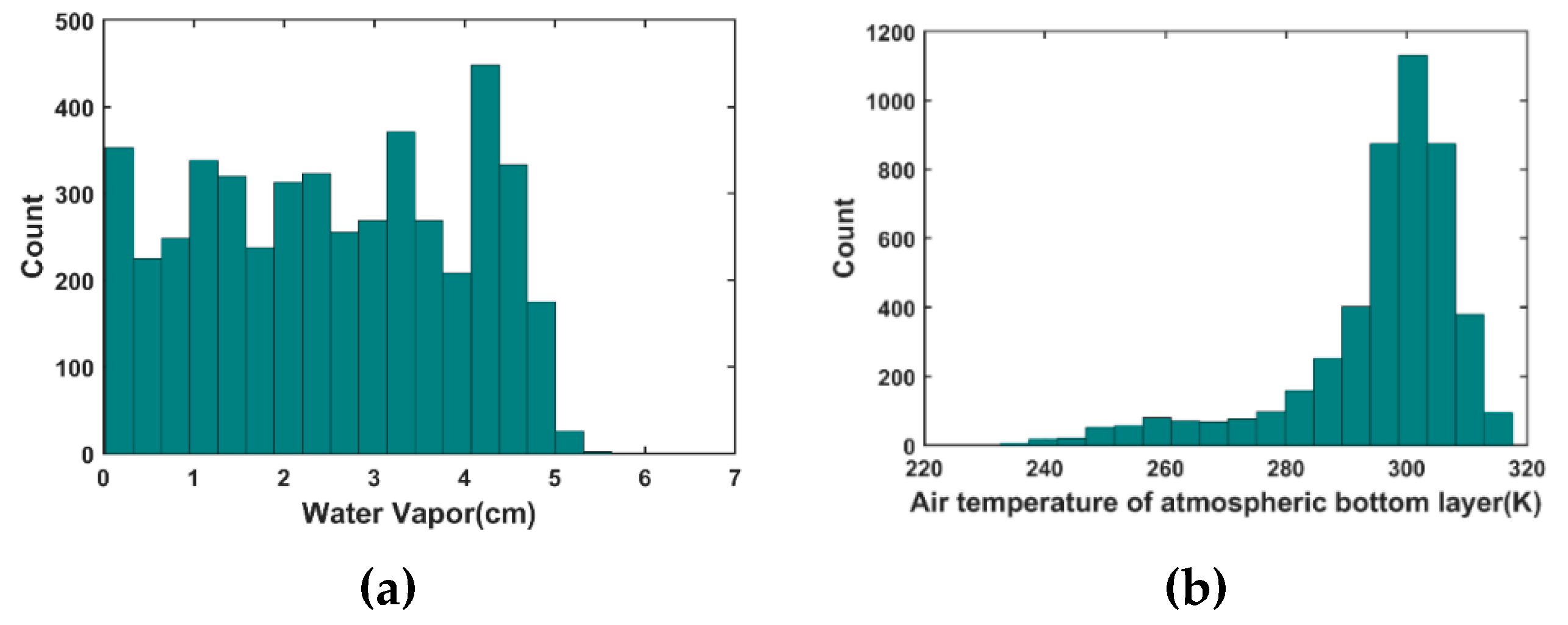
To obtain the coefficients, the Global Atmospheric Profiles from Reanalysis Information (GAPRI) [33] are used as the input to the moderate spectral resolution atmospheric transmittance model version 5 (MODTRAN 5.0) to generate the brightness temperature of Landsat 8 TIR channels. According to the research of Jiménez-Muñoz et al. [12], 4714 GAPRI atmospheric profiles over land were choose for simulation. The distribution of the total water vapor content (TWV) and the air temperature at the first layer of atmospheric profiles (T0) are shown in Figure 1. The water vapor is evenly distributed in the range of 0–5 cm, which indicates that the atmospheric profiles used are highly representative. For a realistic simulation using limited atmospheric profiles, we followed Jiménez-Muñoz et al. [12,34] and set the LSTs as: T0 − 5, T0, T0 + 5, T0 + 10, T0 + 15, and T0 + 20. Moreover, 110 emissivity spectra from the Advanced Spaceborne Thermal Emission and Reflection Radiometer (ASTER) [35] and Moderate Resolution Imaging Spectroradiometer (MODIS) spectral library [36] were also selected. Among them, there are 19 vegetation types, 39 soil types, 5 snow/water types, 35 rock types, and 12 manmade material types. In total, 3, 111, and 240 different groups of simulated data are obtained (4714 profiles × 110 emissivity spectra × 6 temperatures). Finally, the coefficients $C_i$ (I = 0–7) in Equations (1)–(3) were determined by a least squares regression.

2.3. Land Surface Emissivity Estimation

The empirical relationships between thermal infrared parameters and optical parameters were established long before. For example, Menenti et al. [37] reported a linear relationship between field-measured surface temperature and reflectance over nonhomogeneous surface types. Van De Griend and Owe [38] found that emissivity has a good logarithmic relationship with the normalized difference vegetation index (NDVI). Cheng et al. [39] proposed the method of predicting broadband emissivity of non-vegetated surfaces with spectral albedos. Recently, the study of Cheng et al. [40] indicated that there is a physical linkage between land surface emissive and reflective variables over non-vegetated surfaces, which provides a theoretical perspective on estimating land surface emissivity for sensors with only one or two thermal infrared channels. Thus, the improved NDVI-based threshold method proposed by Tang et al. [41] was selected to estimate the Landsat 8 LSE of the non-vegetated area. According to the research of Emami et al. [42], the performance of this linear relationship is better than the constant assumption or a linear function fitting the red reflectance adopted by the NDVI threshold. For vegetated area, the vegetation cover method of Valor and Caselles [43] was selected. The expression for calculating LSE is provided as below:

$${\mathsf{\epsilon }}_i=\{\begin{array}{c}{a}_{1i}+{\displaystyle {\displaystyle \sum }_{j=2}^7}{a}_{ji}{\rho }_j NDVI<NDV{I}_s\\ {\epsilon }_{vi}{P}_v+{\epsilon }_{si}\left(1-P_v\right)+4d\epsilon P_v\left(1-P_v\right) NDV{I}_s\le NDVI\end{array}$$

(4)

where ${\mathsf{\epsilon }}_i$ is the LSE in band 10 or band 11; ${\epsilon }_{vi}$ and ${\epsilon }_{si}$ are the vegetation component emissivity and background component emissivity, respectively; ${\rho }_j$ is the surface reflectance of the Operational Land Imager (OLI)band j; $a_{ji}$ is coefficient (j = 1~7); and $P_v$ is the fractional vegetation cover, which can be expressed by [44]:

$$P_v={\left[\frac{NDVI-NDV{I}_s}{NDV{I}_v-NDV{I}_s}\right]}^2$$

(5)

where $NDV{I}_v$ and $NDV{I}_s$ are the NDVI for the bare soil pixels and fully vegetated pixels, respectively. To maintain the spatial consistency, $NDV{I}_s=0.2$ and $NDV{I}_v=0.86$ are assigned [45,46]. Moreover, $d\epsilon$ represents the emissivity increment from the cavity effect caused by the multiple scattering in the pixel, and can be expressed by [47]:

$$d\epsilon =\{\begin{array}{l}\frac{{\epsilon }_{vi}\left(-0.435{\epsilon }_{si}+0.4343\right)}{0.985} {\epsilon }_{vi}\ne 0.985\\ -0.435{\epsilon }_{si}+0.4343 {\epsilon }_{vi}=0.985\end{array}$$

(6)

2.4. Ground LST Estimation

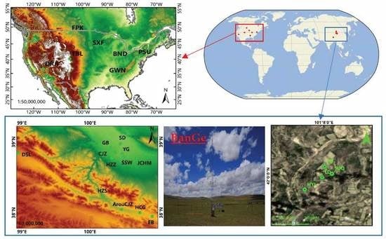
To test the accuracy of the enterprise algorithm, a total of twenty four in situ sites of Surface Radiation Budget Monitoring (SURFRAD) [48,49] in the USA or Heihe Watershed Allied Telemetry Experimental Research (HiWATER) [50,51] in China were chosen to validate the estimated LST. Those sites contain seven SURFRAD sites, four sites in HiWATER downstream (hereafter refered to as HiWATER_A), seven sites in HiWATER midstream, and one Da Sha Long (DSL) site (hereafter refered to as HiWATER_B), four sites in HiWATER upstream (hereafter referred to as HiWATER_C). Ground-measurements from SURFRAD and HiWATER have been widely used to validate LST products [52,53,54]. In addition, one in situ site (BanGe) in the Third Tibetan Plateau Atmospheric Scientific Experiment (TIPEX-III) [55] was selected for validation. TIPEX-III has eleven in situ sites, we only obtained matched Landsat 8 data over the GanGe site. The geographic locations of the twenty-four in situ sites are presented in Figure 2.

Table 1. In-situ sites’ information and the corresponding path/row of Landsat 8.

	Site	Name	Latitude	Longitude	Land Cover	Period	Path/Row
SURFRAD	BND	Bondville	40.0519	−88.3731	cropland	2013~2018	23/32
	GWN	Goodwin Creek	34.2547	−89.8729	grassland	2013~2018	23/36
	PSU	Penn. State	40.7201	−77.9309	cropland	2013~2018	16/32
	SXF	Sioux Falls	43.7343	−96.6233	grassland	2013~2018	29/30
	FPK	Fort Peck	48.3079	−105.1018	grassland	2013~2018	35/26
	TBL	Table Mountain	40.1256	−105.2378	sparse grassland	2013~2018	33/32
	DRA	Desert Rock	36.6232	−116.0196	arid shrubland	2013~2018	40/35
HiWATE_A	HYL	Hu Yang Lin	41.9932	101.1239	populus forest	2013~2015	133/031
	LD	Luo Di	41.9993	101.1326	barren-land	2013~2015
	NT	Nong Tian	42.0048	101.1338	cropland	2013~2015
	SDQ	Si Dao Qiao	42.0012	101.1374	tamarix	2013~2017
HiWATER_B	GB	Ge Bi	38.9150	100.3042	gobi desert	2013~2015	133/033
	SSW	Shen Sha Wo	38.7892	100.4933	sand dune	2013~2015
	JCHM	Ji Chang Huang Mo	38.7781	100.6967	desert steppe	2013~2015
	SD	Shi Di	38.9751	100.4464	reed wetland	2013~2017
	CJZ	Chao Ji Zhan	38.8555	100.3722	corn	2013~2017
	HZZ	HuaZhaiZi	38.7659	100.3201	desert steppe	2013~2017
	YG	YaoGan	38.8270	100.4756	artificial grass	2015~2017
	DSL	Da Sha Long	38.8399	98.9406	marsh	2013~2017	134/033
HiWATER_C	ArouCJZ	Arou Chao Ji Zhan	38.0473	100.4643	alpine meadow	2013~2017	133/034
	EB	Er Bao	37.9492	100.9151	alpine meadow	2013~2016
	HZS	Huang Zang Si	38.2254	100.1918	wheat	2013~2015
	HCG	Huang Cao Gou	38.0033	100.7312	alpine meadow	2013~2015
TIPEX-III	BG	BanGe	31.4200	90.0300	alpine meadow	20140712~20140903	138/038 139/038

SURFRAD: Surface Radiation Budget Monitoring sites; HiWATER_A: Heihe Watershed Allied Telemetry Experimental Research (HiWATER) downstream sites; HiWATER_B: HiWATER midstream sites and Da Sha Long (DSL) site; HiWATER_C: HiWATER upstream sites; TIPEX-III: BanGe site in the Third Tibetan Plateau Atmospheric Scientific Experiment.

shows the in-situ sites’ information (e.g., latitude, longitude, land cover type) and the corresponding path/row of Landsat 8.

For the Ji Chang Huang Mo (JCHM) site, the radiation temperatures measured by the SI-111 radiometer were used to calculate the in-situ LSTs, and the formula is given by Equation (6). The effects of emissivity and the downward sky irradiance were corrected.

$$B(T_{\mathrm{s}})=\left[B(T_r)-(1-\epsilon )L_{\mathrm{sky}}\right]/\epsilon$$

(7)

where $T_{\mathrm{s}}$ is the LST, $T_r$ is the radiation temperature, $B$ is the plank function, $\epsilon$ is the emissivity of SI-111 channel, $L_{\mathrm{sky}}$ is the downwelling atmospheric radiance.

For other sites, the LST was estimated from the upwelling and downwelling longwave radiation using the following equation:

$$T_s={\left[\frac{F^{\uparrow }-\left(1-{\epsilon }_b\right)F^{\downarrow }}{{\epsilon }_b\sigma }\right]}^{0.25}$$

(8)

where T_s is the LST, $F^{\uparrow }$ is the measured surface upwelling longwave radiation, ${\epsilon }_b$ is the surface broadband emissivity (BBE), σ is the Stefan–Boltzmann’s constant (5.67 × 10⁻⁸ Wm⁻²K⁻⁴), and $F^{\downarrow }$ is the measured atmospheric downwelling longwave radiation. The BBE is estimated from the ASTER GED product using the following linear equation according to Cheng et al. [56]:

$${\epsilon }_b=0.197+0.025{\epsilon }_{10}+0.057{\epsilon }_{11}+0.237{\epsilon }_{12}+0.333{\epsilon }_{13}+0.146{\epsilon }_{14}$$

(9)

where ${\epsilon }_b$ is the surface broadband emissivity, and ${\epsilon }_{10}$–${\epsilon }_{14}$ are the ASTER narrowband emissivities of five channels.

3. Results and Analyses

3.1. Algorithm Coefficients

As described in Section 2.2, GAPRI atmospheric profiles were used to derive the coefficients of the algorithms, whereas the Cloudless Land Atmosphere Radiosounding (CLAR) [57] with 382 profiles, Thermodynamic Initial Guess Retrieval (TIGR) [58] with 946 profiles, and 2762 SeeBor V5.0 global profiles (hereafter SeeBor) [59] were used for validation purposes. All the profiles are restricted to land under clear sky conditions [60] based on the method of Galve et al. [57]. To improve the inversion accuracy of the land surface temperature, the coefficients of the enterprise algorithm were fitted based on the water vapor content, as shown in

Table 2. Coefficients and uncertainty of the Enterprise algorithm, Wan, and Sobrino under different water vapor content subranges.

TWV(cm)	Method	C0	C1	C2	C3	C4	C5	C6	C7	RMSE(K)
0.0–2.5	Wan	−1.56	1.007	0.162	−0.288	3.179	6.864	−11.209	0.165	0.44
	Enterprise algorithm	54.95	1.01	1.557	−57.805	0.147	−103.52	-	-	0.481
	Sobrino	−0.39	2.116	−0.045	64.386	−3.7	−147.522	21.065	-	0.431
2.0–3.5	Wan	−0.099	0.998	0.148	−0.252	5.236	5.488	−5.455	0.02	0.57
	Enterprise algorithm	50.035	1.006	5.377	−52.801	−3.16	−87.906	-	-	0.589
	Sobrino	−1.631	2.681	-0.054	67.827	−3.213	-204.953	41.441	-	0.503
3.0–4.5	Wan	9.622	0.961	0.121	−0.175	6.611	5.747	−9.262	0	0.709
	Enterprise algorithm	45.395	0.968	8.09	−37.955	−5.312	−70.798	-	-	0.723
	Sobrino	−2.767	3.171	−0.05	51.397	−0.151	−210.415	37.574	-	0.691
4.0–5.5	Wan	15.209	0.937	0.092	−0.104	8.228	8.091	−13.697	−0.064	0.688
	Enterprise algorithm	32.395	0.942	12.365	−17.99	−9.291	−58.571	-	-	0.716
	Sobrino	−4.399	3.969	-0.113	34.649	2.335	−200.753	32.846	-	0.728
5.0–7.0	Wan	7.239	0.962	0.065	−0.054	7.942	8.838	−15.162	−0.001	0.71
	Enterprise algorithm	17.191	0.968	11.816	−11.396	−8.402	−47.408	-	-	0.722
	Sobrino	−5.096	3.932	−0.044	−4.701	8.634	−219.875	33.98	-	0.743
0.0–7.0	Wan	−2.64	1.012	0.142	−0.201	2.844	−0.569	−7.6	0.263	0.844
	Enterprise algorithm	67.297	0.985	−6.916	−63.855	9.548	−90.919	-	-	1.075
	Sobrino	−0.717	1.988	0.121	70.148	−7.006	−143.246	19.247	-	0.72

. The water vapor content was divided into five subranges: 0.0–2.5, 2.0–3.5, 3.0–4.5, 4.0–5.5, and 5.0–7.0 cm, with an overlap of 0.5 cm. We derived the coefficients using the samples in each subrange. In addition, the coefficients were also fitted for the entire water vapor content. We also derived the coefficients of Wan and Sobrino with the same method and data.

The RMSE of the estimated LST derived from the Enterprise algorithm were all between 0.48 and 0.72 K under five water vapor subranges, whereas those values were between 0.44 (0.43) and 0.71 K (0.74K) for Wan (Sobrino). Under full water vapor range, RMSEs were 1.08, 0.84, and 0.72 K for the Enterprise algorithm, Wan, and Sobrino, respectively. The uncertainty of the algorithm of Sobrino is slightly lower than that of Wan and the enterprise algorithm in low water vapor content subrange. For high water vapor content subrange, the uncertainty of the algorithm of Wan is slightly lower than that of the enterprise algorithm and Sobrino.

The bias and RMSE of the Enterprise algorithm, Wan, and Sobrino tested by three independent simulated datasets are shown in

Table 3. The bias and RMSE of three split-window algorithms when tested by three independent atmospheric profiles. W1–W6 is the atmospheric water vapor range (W1 = 0.0–2.5 cm; W2 = 2.0–3.5 cm; W3 = 3.0–4.5 cm; W4 = 4.0–5.5 cm; W5 = 5.0–7.0 cm, and W6 = 0.0–7.0 cm).

	Data	Method	W1	W2	W3	W4	W5	W6
bias(K)	CLAR	WAN	0.057	−0.008	−0.029	0.107	−0.307	−0.022
		Enterprise algorithm	0.142	0.058	−0.017	−0.075	−0.051	−0.031
		Sobrino	0.193	0.065	−0.040	−0.167	−0.249	−0.140
	TIGR	WAN	−0.121	−0.035	0.034	−0.04	−0.180	−0.085
		Enterprise algorithm	−0.055	0.028	0.049	−0.158	0.078	−0.155
		Sobrino	0.138	0.032	0.013	−0.261	−0.106	0.058
	SeeBor	WAN	0.129	0.164	0.284	0.430	−0.085	0.150
		Enterprise algorithm	0.197	0.230	0.299	0.263	0.174	−0.005
		Sobrino	0.228	0.283	0.330	0.236	0.006	0.177
RMSE(K)	CLAR	WAN	0.430	0.527	0.651	0.739	0.920	1.007
		Enterprise algorithm	0.498	0.544	0.662	0.742	0.874	1.417
		Sobrino	0.540	0.479	0.607	0.762	0.922	1.022
	TIGR	WAN	0.357	0.608	0.735	0.945	1.205	0.724
		Enterprise algorithm	0.420	0.619	0.757	0.930	1.202	0.923
		Sobrino	0.594	0.513	0.762	0.997	1.175	0.810
	SeeBor	WAN	0.429	0.621	0.753	0.925	1.132	0.750
		Enterprise algorithm	0.523	0.659	0.765	0.866	1.143	1.038
		Sobrino	0.578	0.628	0.762	0.863	1.139	0.779

CLAR: Cloudless Land Atmosphere Radiosounding; TIGR: Thermodynamic Initial Guess Retrieval; SeeBor: SeeBor V5.0 global profiles.

. When tested by the CLAR atmospheric profile, the biases (RMSEs) of the Enterprise algorithm were between −0.08 (0.50) and 0.14 K (1.42 K). For Wan and Sobrino, the biases (RMSEs) were between −0.31(0.43) and 0.19 K (1.01 K). When tested by TIGR atmospheric profile, the biases (RMSEs) of the Enterprise algorithm were between −0.16 (0.42) and 0.08 K (1.20 K). For Wan and Sobrino, the biases (RMSEs) were between −0.26 (0.36) and 0.14 K (1.21 K). Regarding the SeeBor atmospheric profile, the biases (RMSEs) of Enterprise algorithm were between −0.01 (0.52) and 0.30 K (1.14 K), whereas the biases (RMSEs) were between −0.09 (0.43) and 0.43 K (1.13 K) for Wan, and 0.01 (0.58) and 0.33 K (1.14 K) for Sobrino. According to the test results, we are convinced that the coefficients are accurate and can be used to retrieve LSTs using the split-window algorithms.

3.2. Sensitivity Analysis

As noted by Wan and Dozier [1], the sensor noise, land surface emissivity, and water vapor content are three primary uncertainties that cause errors in LST estimates using the split-window algorithm. Therefore, we evaluated the algorithms’ sensitivity to the above three variables.

3.2.1. Sensor Noise

The effect of sensor noise on LST uncertainty $\delta T_S$ can be expressed by the following equation:

$$\begin{array}{l}\delta T_{S-Y\mathrm{u}}=\sqrt{{((C_1+C_2+C_4\epsilon )\delta B{T}_{10})}^2+{((-C_2-C_4\epsilon )\delta B{T}_{11})}^2}\\ \delta T_{S-\mathrm{wan}}=\sqrt{{(0.5(C_1+C_2\frac{1-\epsilon }{\epsilon }+C_3\frac{△\epsilon }{{\epsilon }^2})\delta BT)}^2+{((0.5(C_4+C_5\frac{1-\epsilon }{\epsilon }+C_6\frac{△\epsilon }{{\epsilon }^2})+2C_7△BT)\delta (△BT))}^2}\\ \delta T_{S-\mathrm{Sobrino}}=\sqrt{{((1+C_1+2C_2△BT)\delta B{T}_{10})}^2+{((-C_1-2C_2△BT)\delta B{T}_{11})}^2}\end{array}$$

(10)

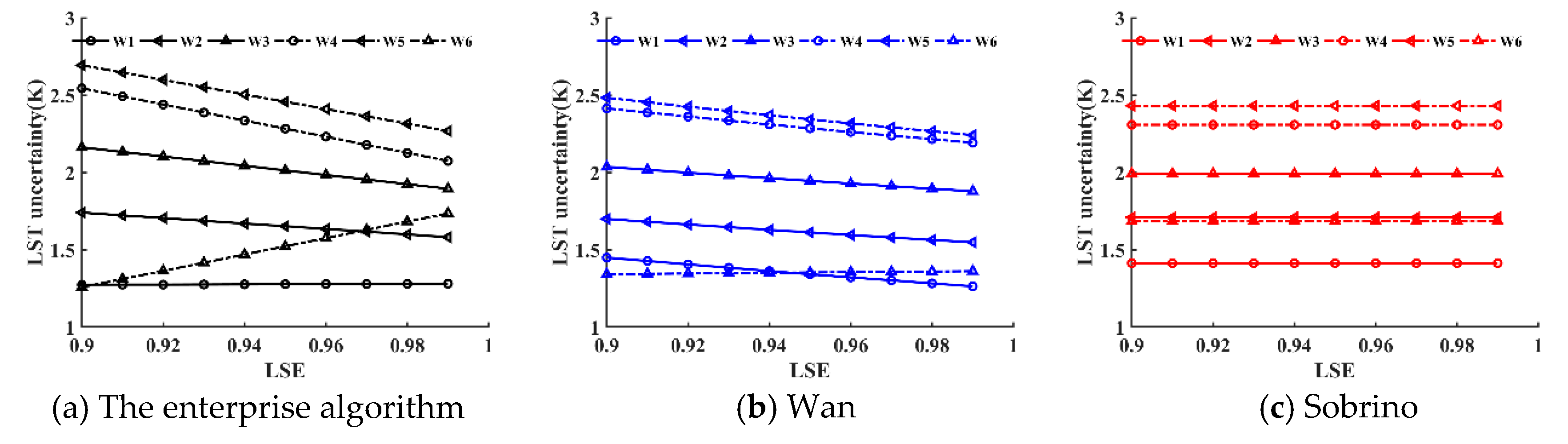
where $\delta B{T}_{10}$ and $\delta B{T}_{11}$ are the noise-equivalent-change-in-temperature ($NE\Delta T$). According to the description of Irons et al. [61], the $NE\Delta T$ of the TIRS instrument onboard the Landsat-8 satellite was designed as 0.4 K at 300 K for band 10 and band 11; therefore, $\delta B{T}_{10}$ and $\delta B{T}_{11}$ are set as 0.4 in this study. $\delta BT=\delta (△BT)=\sqrt{\delta B{T}_{{}_{10}}^2+\delta B{T}_{{}_{11}}^2}$ [62]. $\epsilon$ is the mean emissivity of band 10 and band 11. The mean emissivity was set from 0.9 to 0.99 with a step of 0.01. $C_{\mathrm{i}}$ are the algorithm coefficients in Table 2.

The LST uncertainty attributed to the sensor noise at six water vapor content subranges (W1–W6) is shown in Figure 3. The results indicate that three split-window algorithms have similar LST uncertainty under various water vapor content subranges. The LST uncertainty of the Enterprise algorithm and Wan decreases with the increase of average emissivity under five water vapor content subranges (W1–W5), but LST uncertainty of Sobrino remain unchanged. For example, LST uncertainty incurred by 0.4K $NE\Delta T$ changed from 1.74 K (1.70 K) to 1.58 K(1.55 K) for the Enterprise algorithm (Wan) and 1.71 K for Sobrino when the water vapor content was 2.0–3.5 cm. However, under full water vapor content, LST uncertainty increased with the increase of average emissivity, 0.4 K $NE\Delta T$ can cause LST uncertainty ranging from 1.26 K(1.34 K) to 1.74 K(1.36 K) for the Enterprise algorithm (Wan) and 1.69 K for Sobrino.

3.2.2. Emissivity Uncertainty

The LST uncertainty attributed to the emissivity uncertainty $\delta T_{\epsilon }$ can be expressed by the following equation:

$$\begin{array}{c}\delta T_{\epsilon -\mathrm{yu}}=\sqrt{{((C_3+C_4(T_{10}-T_{11}))\delta \epsilon )}^2+{(C_5\delta (\Delta \epsilon ))}^2}\\ \delta T_{\epsilon -\mathrm{wan}}=\sqrt{\begin{array}{l}{((-(C_2\frac{T_{10}+T_{11}}{2}+C_5\frac{T_{10}-T_{11}}{2})/{\epsilon }^2-2(C_3\frac{T_{10}+T_{11}}{2}+C_6\frac{T_{10}-T_{11}}{2})\Delta \epsilon /{\epsilon }^3)\delta \epsilon )}^2\\ +{((C_3\frac{T_{10}+T_{11}}{2}+C_6\frac{T_{10}-T_{11}}{2})/{\epsilon }^2\delta (\Delta \epsilon ))}^2\end{array}}\\ \delta T_{\epsilon -\mathrm{sobrino}}=\sqrt{{(-(C_3+C_4\mathrm{w})\delta \epsilon )}^2+{((C_5+C_6\mathrm{w})\delta (\Delta \epsilon ))}^2}\end{array}$$

(11)

where $\delta \epsilon$ and $\delta (\Delta \epsilon )$ are the mean emissivity uncertainty and the uncertainty of channel emissivity difference, respectively. Assuming the emissivity uncertainties in each band are the same, i.e., $\Delta \epsilon$ = $\Delta {\epsilon }_{10}$ = $\Delta {\epsilon }_{11}$, the maximum emissivity difference uncertainty is $\delta (\Delta \epsilon )=\left|\delta {\epsilon }_{10}\right|+\left|\delta {\epsilon }_{11}\right|=2\delta \epsilon$. Although the uncertainty of surface emissivity is often set to 0.01 [12,34], as indicated by Sobrino et al. [63], it is worthwhile to analyze other reference uncertainties in surface emissivity. In this case, $\delta \epsilon$ was set from 0 to 0.03 with a step of 0.005. $C_{\mathrm{i}}$ are the algorithm coefficients in Table 2.

Figure 4 shows the LST uncertainty attributed to the emissivity uncertainty. The results indicate that LST uncertainty of three split-window algorithms increases with the emissivity uncertainty, but the increase ratio slows down as the water vapor content increases. The LST uncertainty of Sobrino is slightly higher than that of the Wan and Enterprise algorithms when the water vapor content subrange was 0.0–2.5 cm, and LST uncertainty of the Enterprise algorithm was slightly higher than that of Sobrino and Wan when water vapor content subrange was 4.0–5.5 cm, 5.0–10.0 cm, and 0.0–10.0 cm. For example, an emissivity uncertainty of 0.01 can cause LST uncertainty of 2.5 K for Sobrino, 2.18 K for Wan, and 2.15 K for the Enterprise algorithm when the water vapor range was 0.0–2.5 cm; the LST uncertainty ranging from 0.99 to 1.22 K for the Enterprise algorithm, 0.72 to 1.02 K for Wan, and 0.92 to 1.01 K for Sobrino when water vapor content was larger than 4.0 cm, respectively. This result also indicates that LST uncertainty of split-window algorithm is sensitive to the emissivity uncertainty in dry atmospheric conditions. In other words, the change of the land surface in dry atmospheric conditions could introduce a large error in the LST retrieval.

3.2.3. Water Vapor Content

The LST uncertainty attributed to the water vapor content was primarily caused by incorrect selection of the TWV subrange. Assuming the error of TWV is 0.5 cm [46,64], the LST at a certain water vapor subrange can be retrieved using coefficients obtained from adjacent water subranges. The RMSEs of LST retrieval due to using coefficients of the adjacent TWV subrange are shown in

Table 4. RMSEs of LST retrieval due to incorrectly using of coefficients of the adjacent total water vapor content (TWV) subrange.

True TWV Subrange (cm)	Method	Used TWV Subrange (cm)
		0.0–2.5	2.0–3.5	3.0–4.5	4.0–5.5	5.5–7.0
0.0–2.5	Wan	0.440 K	1.422 K	-	-	-
	Sobrino	0.431 K	0.771 K	-	-	-
	Enterprise algorithm	0.481 K	1.377 K	-	-	-
2.0–3.5	Wan	0.891 K	0.570 K	1.232 K	-	-
	Sobrino	0.795 K	0.503 K	0.851 K	-	-
	Enterprise algorithm	1.057 K	0.589 K	1.207 K	-	-
3.0–4.5	Wan	-	1.104 K	0.709 K	1.062 K	-
	Sobrino	-	1.053 K	0.691 K	0.930 K	-
	Enterprise algorithm	-	1.121 K	0.723 K	1.063 K	-
4.0–5.5	Wan	-	-	0.938 K	0.688 K	1.033 K
	Sobrino	-	-	0.900 K	0.728 K	0.987 K
	Enterprise algorithm	-	-	0.944 K	0.716 K	0.980 K
5.5–7.0	Wan	-	-	-	1.014 K	0.710 K
	Sobrino	-	-	-	1.017 K	0.743 K
	Enterprise algorithm	-	-	-	0.960 K	0.722 K

. As shown in Table 4, the incorrect selection of the TWV subrange led to a significant increase in LST retrieval. For example, if TWV is equal to 2.8 cm, which belongs to a subrange of 2.0–3.5 cm, the RMSE of Wan, Sobrino, and the Enterprise algorithm are 0.570, 0.503, and 0.589 K. When coefficients in a subrange of 0.0–2.5 cm are used, the RMSE increases to 0.891, 0.795, and 1.057 K; when using coefficients in a subrange of 3.0–4.5 cm, the RMSE becomes 1.232, 0.851, and 1.207 K. It is worth noting that mis-classification of TWV led to a larger LST uncertainty in dry atmospheric conditions than in wet atmospheric conditions, e.g., in the previous example, the RMSE increased by 79.5% and 104.9% for the Enterprise algorithm. When TWV belongs to a subrange of 0.0–2.5 cm and the coefficients of a subrange of 2.0–3.5 cm were improperly used, the RMSE increased by 223.2%, 78.9%, and 186.3% for Wan, Sobrino, and the Enterprise algorithm.

3.2.4. Total Error

According to the research of [34,62], the total LST uncertainty $e(\mathrm{LST})$ can be calculated by:

$$e(\mathrm{LST})=\sqrt{\delta T_s^2+\delta T_{\epsilon }^2+\delta T_w^2+\delta T_{a\lg }^2}$$

(12)

where $\delta T_{a\lg }$ is the algorithm uncertainty, $\delta T_S$, $\delta T_{\epsilon }$ and $\delta T_{\mathrm{w}}$ are the LST uncertainty attributed to the sensor noise, emissivity uncertainty, and water vapor content uncertainty, respectively. Assuming the land surface temperature is 300 K, the mean emissivity is 0.96 and total water vapor equals to 1.5 cm. Given an emissivity error equal to 0.01 and $NE\Delta T$ equals to 0.4 K, the total LST uncertainty retrieval using Equation (12) is 2.59, 2.62, and 2.93 K for the Enterprise algorithm, Wan, and Sobrino when using the correct coefficients in a subrange of 0.0–2.5 cm. When the coefficients in subrange of 2.0–3.5 cm was used, the total LST uncertainties are 2.90, 2.95, and 3.00 K for the Enterprise algorithm, Wan, and Sobrino. The results show that if the emissivity error and sensor noise are known, the TWV error has little effect on the total LST uncertainty. In other words, sensor noise and emissivity error are the main error sources in the split-window algorithm, which is consistent with the result of Chen et al. [28] and Sobrino et al. [65].

3.3. Validate with the In Situ LST

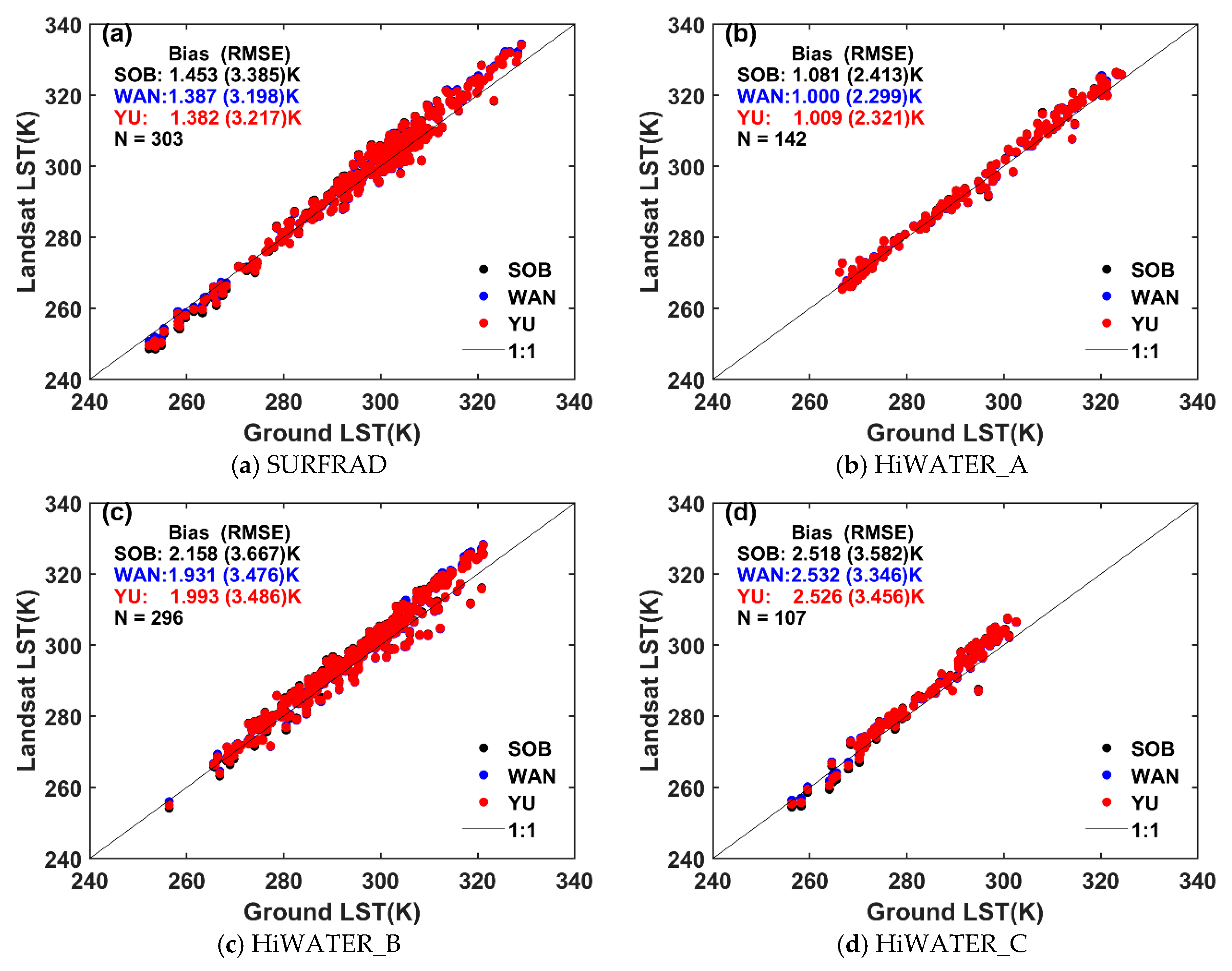
The coefficients of the split-window algorithms are selected based on the water vapor content calculated from the Modern-Era Retrospective Analysis for Research and Applications, Version 2 (MERRA-2) reanalysis product. The cloud mask is calculated from the quality assessment (QA) band of Landsat 8 Level-2 surface reflectance data. Land surface emissivity is calculated using the method described in Section 2.3. The retrieved Landsat LSTs are compared with the ground-measured LSTs. Figure 5 shows the scatterplot of ground-measured LSTs and retrieved LSTs. The LSTs are overestimated at SURFRAD and HiWATER sites. At the SURFRAD sites, the biases (RMSEs) of the LSTs retrieved by the Enterprise algorithm, Wan, and Sobrino are 1.38 (3.22), 1.39 (3.20), and 1.45 K (3.39 K), respectively. At the HiWATER_A sites, three split-window algorithms have similar accuracy and uncertainty, the biases and RMSEs are about 1.0 K and 2.3 K. Regarding the HiWATER_B sites, the Enterprise algorithm and Wan have similar performance, with a bias (RMSE) of 0.2 K lower than that of Sobrino. For the HiWATER_C sites, Wan, the Enterprise algorithm and Sobrino have similar bias and RMSE, the biases and RMSEs are 2.5 K and 3.4 K. The bias and RMSE of LST retrieved from three split-window algorithms in BanGe site are shown in

Table 5. Biases and RMSEs of retrieved LST at the BanGe site.

Date	In Situ (K)	Enterprise Algorithm (K)	Wan (K)	Sobrino (K)
27 July 2014	300.29	300.30	300.10	300.38
12 August 2014	296.13	293.98	293.78	294.15
28 August 2014	295.73	296.05	295.83	296.26
18 July 2014	294.27	295.45	295.29	295.72
19 August 2014	298.8	298.70	298.47	298.82
BIAS(K)		−0.15	−0.35	0.02
RMSE(K)		1.11	1.16	1.12

, which indicated that the accuracy and uncertainty of three split-window algorithms are similar in BanGe site. The biases are −0.15, −0.35 and 0.02 K, whereas the RMSEs are 1.11, 1.16 and 1.12 K for the Enterprise algorithm, Wan and Sobrino, respectively.

According to the validation results, we can conclude that the enterprise algorithm can achieve a high precision in estimating LST, and have comparable accuracy with the generalized split-window algorithm (Wan) and the algorithm of Sobrino (Sobrino).

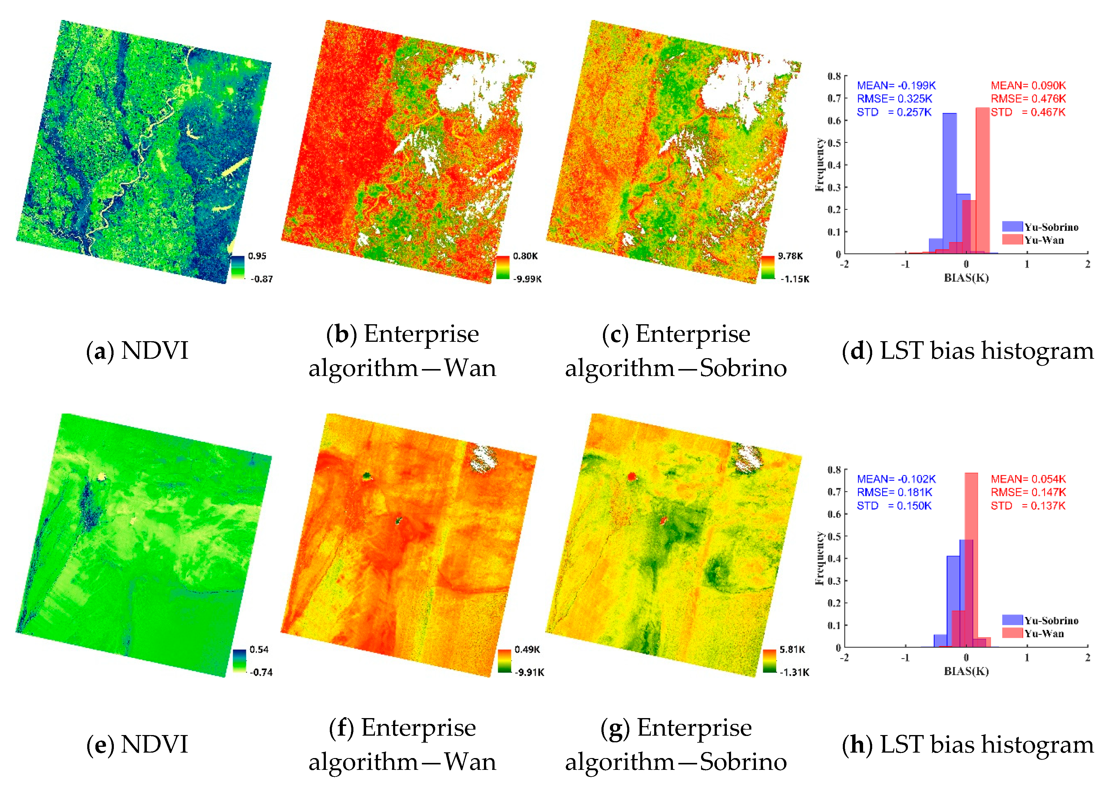
For a more intuitive comparison, two days of Landsat-8 images containing less cloudiness acquired on 2 May 2014 (path/row: 023/036) and 5 May 2014 (path/row: 133/031) were selected to analyze the spatial distribution of retrieved LSTs. Images of LST differences, the corresponding histograms of LST bias, and NDVI images are shown in Figure 6.

In Figure 6a, 90.6% of the NDVI value are larger than 0.2. This area can be regarded as vegetated area according to the research of references [45,46]. For the vegetation area, the average LSTs retrieved from the Enterprise algorithm are slightly higher than those from Wan, and the average bias, RMSE, and standard deviation (SD) are 0.09, 0.48, and 0.47 K, respectively. The average LSTs retrieved from the Enterprise algorithm were slightly lower than those from Sobrino, and the average bias, RMSE, and SD were −0.20, 0.33, and 0.26 K, respectively. For the non-vegetation area, 98.85% of the NDVI values were between 0.019 and 0.117 (Figure 6e). The difference between the three split-window algorithms were slightly lower than that in the vegetation area. The average bias was 0.05 K (−0.10 K) and the RMSE was 0.15 K (0.18 K) for the Enterprise algorithm minus Wan (Sobrino). Although from the legends in Figure 6f,g, there is a large deviation in the LST image, 99.77% of the biases ranged from −0.63 K and 0.27 K. Moreover, the large biases were located in the pixels surrounded by clouds. The result indicated that the enterprise algorithm could achieve a similar accuracy to the generalized split-window algorithm (Wan) and the split-window algorithm of Sobrino et al. [32] over the vegetation and non-vegetation areas.

4. Discussion

In this section, we compare the enterprise algorithm with the results of other studies. For example, Zhang et al. [66] validated Landsat 8 LSTs retrieved from a single-channel algorithm proposed by Jiménez-Muñoz et al. [12] (hereafter JMS) using SURFRAD sites. The bias, mean absolute error (MAE), and RMSE of the JMS method are 1.49, 1.57, and 1.96 K, respectively. We selected the same 21 Landsat-8 images in SURFRAD as Zhang et al. [66], and the validation results indicated the Enterprise algorithm, Wan and Sobrino have similar performance. The biases (RMSEs) were 0.85 (2.34), 0.74 (2.28), and 0.94 K (2.46 K) for the Enterprise algorithm, Wan, and Sobrino, respectively.

Yu et al. [67] compared three different approaches for LST inversion, including the radiative transfer equation algorithm applied to band 10 (hereafter RTE10) and band 11 (hereafter RTE11), the split-window algorithm proposed by Qin et al. [68] (hereafter Qin) and the single-channel method proposed by Jiménez-Muñoz et al. [19] applied to band 10 (hereafter JMS10) and band 11 (hereafter JMS11). The LST derived by RTE applied to band 10 in our result is called RTE_M, hereafter. In RTE_M, the MERRA2-6 reanalysis product was used for atmospheric correction. We have selected 20 images, all of which exist in our work and in the study of Yu et al. The biases (RMSEs) between the retrieved LSTs using various methods and in-situ LSTs are shown in

Table 6. Biases and RMSEs of LST retrieval with various methods.

	RTE10	RTE11	Qin	JMS10	JMS11	RTE_M	Wan	Enterprise Algorithm	Sobrino
BIAS(K)	−0.95	−0.96	−1.28	−0.92	−0.51	1.00	1.85	1.90	2.08
RMSE(K)	2.95	3.05	3.02	3.04	3.10	2.61	2.95	2.93	3.09

. The results show that the LSTs retrieved from the RTE method (RTE10, RTE11, and RTE_M) and the single-channel algorithm (JMS10 and JMS11) have the higher accuracy with a bias lower than 1K, while four split-window algorithms (Qin, Wan, the Enterprise algorithm, and Sobrino) have low precision with bias (RMSE) that varies between −1.28 K (2.93 K) and 2.08 K (3.09 K). The accuracy of the Enterprise algorithm, Wan, and Sobrino are similar, and the biases (RMSEs) are 1.90 K (2.93 K), 1.85 K (2.95 K) and 2.08 K (3.09 K), respectively.

García-Santos et al. [27] also compared three methods for estimating the LST from Landsat-8 data, including RTE10, RTE11, the single-channel algorithm proposed by Jiménez-Muñoz et al. [19] (hereafter JMS) and Wang et al. [13] (hereafter Wang) and the split-window algorithm proposed by Jiménez-Muñoz et al. [12] (hereafter JM2014), and Du et al. [14] (hereafter Du). The result of García-Santos and our result using 21 Landsat-8 scenes in Mallorca Island is shown in

Table 7. Biases and RMSEs of LST retrieval with various methods.

	RTE10	RTE11	JMS	Wang	Du	JM2014	RTE_M	Wan	Enterprise Algorithm	Sobrino
Bias(K)	−0.1	2.0	0.8	0.7	−1.4	0.4	0.1	0.2	0.1	0.2
RMSE(K)	2.3	3.6	2.2	2.3	2.0	1.6	2.3	1.7	1.7	1.7

. The accuracy of RTE_M was nearly the same as that of RTE10, and the bias and RMSE were 0.1 (−0.1) and 2.3 K (2.3 K). The method of Du had higher absolute bias (RMSE) than the Enterprise algorithm, Wan, and Sobrino and the differences were 1.2 and 0.3 K for bias and RMSE. In this validation, the Enterprise algorithm, Wan, and Sobrino achieved similar bias and equal RMSE. Three split-window algorithms and JM2014 achieved a similar accuracy, with a bias and RMSE of 0.2 (0.4) and 1.7 K (1.6 K), respectively. From existing verification results, we can conclude that the precision of the Enterprise algorithm, Wan, and Sobrino had similar accuracy in most cases.

Although the validation accuracy was relatively high, some phenomena in Landsat-8 images are worth mentioning. The striping and banding were still very noticeable, and the LST differences on two sides of the strip were not negligible. In addition, as noted by Gerace and Montanaro [25], even the implementation of the stray light algorithm has improved the performance of the TIRS instrument, and the TIRS sensor will continue to be monitored to ensure the expected radiation accuracy for all users.

In spite of single-channel algorithms having better performance in finite verification results, we recommend split-window algorithms for LST retrieval. The reasons are as follows: As pointed out by Jiménez-Muñoz et al. [12], the split-window algorithm has better results than the single-channel algorithm in theory. Then, Sobrino and Jiménez-Muñoz [69], Jiménez-Muñoz and Sobrino [70], and Li et al. [71] found that all of the single-channel algorithms provide poor results at high atmospheric water vapor contents, and the split-window algorithm performs well over global conditions [12]. In addition, most of the in-situ sites have low water vapor contents, and more ground data needs to be collected for comprehensive analysis, especially in high water vapor content areas.

5. Conclusions

The NOAA JPSS Enterprise algorithm is adapted to Landsat-8 data to obtain the estimate of LST in this study. The improved normalized difference vegetation index-based threshold method was used to estimate the LSE of non-vegetated areas, and the vegetation cover method was adopted to calculate the LSE of vegetated areas. The coefficient of the enterprise algorithm was derived from the simulation dataset using GAPRI atmospheric profiles. Both the simulation dataset and ground measurements were used to test and validate the enterprise algorithm. In addition, the enterprise algorithm was compared to the generalized split-window algorithm and the split-window algorithm of Sobrino.

Simulated datasets derived from three independent atmospheric profiles (CLAR, TIGR, and SeeBor) were used to test the performance of the enterprise algorithm. The biases (RMSEs) of the Enterprise algorithm were between −0.16 (0.42) and 0.30 K (1.42 K), and the biases (RMSEs) of the generalized split-window algorithm were all between −0.31 (0.36) and 0.43 K (1.21 K). For the method of Sobrino, the biases (RMSEs) range from −0.26 (0.48) to 0.33 K (1.18 K).

The in-situ LSTs derived from the flux measurements at SURFRAD, HiWATER sites, and BanGe site were used to validate the Landsat-8 LSTs retrieved by the Enterprise algorithm and other algorithms. The biases (RMSEs) of the Enterprise algorithm were 1.38 (3.22), 1.01 (2.32), 1.99 (3.49), 2.53 (3.46), and −0.15 K (1.11 K) at the SURFRAD, HiWATER_A, HiWATER_B, HiWATER_C sites, and BanGe site, respectively. For the generalized split-window algorithm, the biases (RMSEs) were 1.39 (3.20), 1.0 (2.30), 1.93 (3.48), 2.53 (3.35), and −0.35 K (1.16 K), respectively, whereas those values were 1.45 (3.39), 1.08 (2.41), 2.16 (3.67), 2.52 (3.58), and 0.02 K (1.12 K) for the split-window algorithm of Sobrino.

Both the test and validation results show that the Enterprise algorithm have similar performance with the other two split-window algorithms. Regarding the existing verification results, we can conclude that the Enterprise algorithm can be used to retrieve Landsat-8 LSTs with a similar accuracy to the generalized split-window algorithm and the split-window algorithm of Sobrino. This study provides an alternative method to estimate LSTs from Landsat-8 data.

References

- Wan, Z.; Dozier, J. A generalized split-window algorithm for retrieving land-surface temperature from space. IEEE Trans. Geosci. Remote Sens. 1996, 34, 892–905. [Google Scholar]
- Valor, E.; Caselles, V. Mapping land surface emissivity from ndvi: Application to european, african, and south american areas. Remote Sens. Environ. 1996, 57, 167–184. [Google Scholar] [CrossRef]
- Cheng, J.; Liang, S.; Wang, J.; Li, X. A stepwise refining algorithm of temperature and emissivity separation for hyperspectral thermal infrared data. IEEE Trans. Geosci. Remote Sens. 2010, 48, 1588–1597. [Google Scholar] [CrossRef]
- Weng, Q.; Lu, D.; Schubring, J. Estimation of land surface temperature–vegetation abundance relationship for urban heat island studies. Remote Sens. Environ. 2004, 89, 467–483. [Google Scholar] [CrossRef]
- Manzo-Delgado, L.; Sánchez-Colón, S.; Álvarez, R. Assessment of seasonal forest fire risk using noaa-avhrr: A case study in central mexico. Int. J. Remote Sens. 2009, 30, 4991–5013. [Google Scholar] [CrossRef]
- Guo, G.; Zhou, M. Using modis land surface temperature to evaluate forest fire risk of northeast china. IEEE Geosci. Remote Sens. Lett. 2004, 1, 98–100. [Google Scholar]
- Cheng, J.; Liu, Q.; Li, X.; Qing, X.; Liu, Q.; Du, Y. Correlation-based temperature and emissivity separation algorithm. Sci. China Ser. D Earth Sci. 2008, 51, 363–372. [Google Scholar] [CrossRef]
- Wulder, M.A.; White, J.C.; Loveland, T.R.; Woodcock, C.E.; Belward, A.S.; Cohen, W.B.; Fosnight, E.A.; Shaw, J.; Masek, J.G.; Roy, D.P. The global landsat archive: Status, consolidation, and direction. Remote Sens. Environ. 2016, 185, 271–283. [Google Scholar] [CrossRef]
- Meng, X.; Li, H.; Du, Y.; Liu, Q.; Zhu, J.; Sun, L. Retrieving land surface temperature from landsat 8 tirs data using rttov and aster ged. In Proceedings of the 2016 IEEE International Geoscience and Remote Sensing Symposium, Beijing, China, 10–15 July 2016; pp. 4302–4305. [Google Scholar]
- Cristóbal, J.; Jiménez-Muñoz, J.; Prakash, A.; Mattar, C.; Skoković, D.; Sobrino, J. An improved single-channel method to retrieve land surface temperature from the landsat-8 thermal band. Remote Sens. 2018, 10, 431. [Google Scholar] [CrossRef]
- Wang, M.; Zhang, Z.; He, G.; Wang, G.; Long, T.; Peng, Y. An enhanced single-channel algorithm for retrieving land surface temperature from landsat series data. J. Geophys. Res. 2016, 121, 11712–11722. [Google Scholar] [CrossRef]
- Jimenez-Munoz, J.C.; Sobrino, J.A.; Skokovic, D.; Mattar, C.; Cristobal, J. Land surface temperature retrieval methods from landsat-8 thermal infrared sensor data. IEEE Geosci. Remote Sens. Lett. 2014, 11, 1840–1843. [Google Scholar] [CrossRef]
- Wang, F.; Qin, Z.; Song, C.; Tu, L.; Karnieli, A.; Zhao, S. An improved mono-window algorithm for land surface temperature retrieval from landsat 8 thermal infrared sensor data. Remote Sens. 2015, 7, 4268–4289. [Google Scholar] [CrossRef]
- Du, C.; Ren, H.; Qin, Q.; Meng, J.; Zhao, S. A practical split-window algorithm for estimating land surface temperature from landsat 8 data. Remote Sens. 2015, 7, 647–665. [Google Scholar] [CrossRef]
- Rozenstein, O.; Qin, Z.; Derimian, Y.; Karnieli, A. Derivation of land surface temperature for landsat-8 tirs using a split window algorithm. Sensors (Basel) 2014, 14, 5768–5780. [Google Scholar] [CrossRef] [PubMed]
- Wang, S.; He, L.; Hu, W. A temperature and emissivity separation algorithm for landsat-8 thermal infrared sensor data. Remote Sens. 2015, 7, 9904–9927. [Google Scholar] [CrossRef]
- Cook, M.; Schott, J.; Mandel, J.; Raqueno, N. Development of an operational calibration methodology for the landsat thermal data archive and initial testing of the atmospheric compensation component of a land surface temperature (lst) product from the archive. Remote Sens. 2014, 6, 11244–11266. [Google Scholar] [CrossRef]
- Parastatidis, D.; Mitraka, Z.; Chrysoulakis, N.; Abrams, M. Online global land surface temperature estimation from landsat. Remote Sens. 2017, 9, 1208. [Google Scholar] [CrossRef]
- Jiménez-Muñoz, J.C.; Sobrino, J.A. A generalized single-channel method for retrieving land surface temperature from remote sensing data. J. Geophys. Res. Atmos. 2003, 108, 2015–2023. [Google Scholar] [CrossRef]
- Wang, Y.; Zhou, J.; Li, M.; Zhang, X. Validation of landsat-8 tirs land surface temperature retrieved from multiple algorithms in an extremely arid region. In Proceedings of the 2016 IEEE International Geoscience and Remote Sensing Symposium, Beijing, China, 10–15 July 2016; pp. 6934–6937. [Google Scholar]
- Barsi, J.; Schott, J.; Hook, S.; Raqueno, N.; Markham, B.; Radocinski, R. Landsat-8 thermal infrared sensor (tirs) vicarious radiometric calibration. Remote Sens. 2014, 6, 11607–11626. [Google Scholar] [CrossRef]
- Sobrino, J.; Skoković, D. Permanent stations for calibration/validation of thermal sensors over spain. Data 2016, 1, 10. [Google Scholar] [CrossRef]
- Li, S.; Jiang, G.M. Land surface temperature retrieval from landsat-8 data with the generalized split-window algorithm. IEEE Access 2018, 6, 18149–18162. [Google Scholar] [CrossRef]
- Montanaro, M.; Gerace, A.; Lunsford, A.; Reuter, D. Stray light artifacts in imagery from the landsat 8 thermal infrared sensor. Remote Sens. 2014, 6, 10435–10456. [Google Scholar] [CrossRef]
- Gerace, A.; Montanaro, M. Derivation and validation of the stray light correction algorithm for the thermal infrared sensor onboard landsat 8. Remote Sens. Environ. 2017, 191, 246–257. [Google Scholar] [CrossRef]
- Duan, S.-B.; Li, Z.-L.; Wang, C.; Zhang, S.; Tang, B.-H.; Leng, P.; Gao, M.-F. Land-surface temperature retrieval from landsat 8 single-channel thermal infrared data in combination with ncep reanalysis data and aster ged product. Int. J. Remote Sens. 2018, 1–16. [Google Scholar] [CrossRef]
- García-Santos, V.; Cuxart, J.; Martínez-Villagrasa, D.; Jiménez, M.; Simó, G. Comparison of three methods for estimating land surface temperature from landsat 8-tirs sensor data. Remote Sens. 2018, 10, 1450. [Google Scholar] [CrossRef]
- Chen, Y.; Duan, S.-B.; Ren, H.; Labed, J.; Li, Z.-L. Algorithm development for land surface temperature retrieval: Application to chinese gaofen-5 data. Remote Sens. 2017, 9, 161. [Google Scholar] [CrossRef]
- Caselles, V.; Rubio, E.; Coll, C.; Valor, E. Thermal band selection for the prism instrument: 3. Optimal band configurations. J. Geophys. Res. Atmos. 1998, 103, 17057–17067. [Google Scholar] [CrossRef]
- Guillevic, P.; Göttsche, F.; Nickeson, J.; Hulley, G.; Ghent, D.; Yu, Y.; Trigo, I.; Hook, S.; Sobrino, J.; Remedios, J. Land surface temperature product validation best practice protocol. Version 1.0. Best Pract. Satell. Deriv. Land Prod. Valid. 2017, 60. [Google Scholar] [CrossRef]
- Yu, Y.; Liu, Y.; Yu, P.; Wang, H. Enterprise Algorithm Theoretical Basis Document for Viirs Land Surface Temperature Production; NOAA: Silver Spring, MD, USA, 2017.
- Sobrino, J.A.; Li, Z.-L.; Stoll, M.P.; Becker, F. Multi-channel and multi-angle algorithms for estimating sea and land surface temperature with atsr data. Int. J. Remote Sens. 1996, 17, 2089–2114. [Google Scholar] [CrossRef]
- Mattar, C.; Durán-Alarcón, C.; Jiménez-Muñoz, J.C.; Santamaría-Artigas, A.; Olivera-Guerra, L.; Sobrino, J.A. Global atmospheric profiles from reanalysis information (gapri): A new database for earth surface temperature retrieval. Int. J. Remote Sens. 2015, 36, 5045–5060. [Google Scholar] [CrossRef]
- Jimenez-Munoz, J.-C.; Sobrino, J.A. Split-window coefficients for land surface temperature retrieval from low-resolution thermal infrared sensors. IEEE Geosci. Remote Sens. Lett. 2008, 5, 806–809. [Google Scholar] [CrossRef]
- Baldridge, A.M.; Hook, S.J.; Grove, C.I.; Rivera, G. The aster spectral library version 2.0. Remote Sens. Environ. 2009, 113, 711–715. [Google Scholar] [CrossRef]
- Snyder, W.C.; Wan, Z.; Zhang, Y.; Feng, Y.-Z. Thermal infrared (3–14 um) bidirectional reflectance measurements of sands and soils. Remote Sens. Environ. 1997, 60, 101–109. [Google Scholar] [CrossRef]
- Menenti, M.; Bastiaanssen, W.; Van Eick, D.; El Karim, M.A. Linear relationships between surface reflectance and temperature and their appliation to map actual evaporation of groundwater. Adv. Space Res. 1989, 9, 165–176. [Google Scholar] [CrossRef]
- Griend, A.A.V.D.; Owe, M. On the relationship between thermal emissivity and the normalized difference vegetation index for natural surfaces. Intern. J. Remote Sens. 1993, 14, 1119–1131. [Google Scholar] [CrossRef]
- Cheng, J.; Ren, H.; Liang, S.; Yan, G. Glass-Global Land Surface Broadband Emissivity Product: Algorithm Theoretical Basis Document Version 1.0; Beijing Normal University: Beijing, China, 2010. [Google Scholar]
- Cheng, J.; Liang, S.; Nie, A.; Liu, Q. Is there a physical linkage between surface emissive and reflective variables over non-vegetated surfaces? J. Indian Soc. Remote Sens. 2017, 46, 591–596. [Google Scholar] [CrossRef]
- Tang, B.H.; Shao, K.; Li, Z.L.; Wu, H.; Tang, R. An improved ndvi-based threshold method for estimating land surface emissivity using modis satellite data. Int. J. Remote Sens. 2015, 36, 4864–4878. [Google Scholar] [CrossRef]
- Emami, H.; Mojaradi, B.; Safari, A. A new approach for land surface emissivity estimation using ldcm data in semi-arid areas: Exploitation of the aster spectral library data set. Int. J. Remote Sens. 2016, 37, 5060–5085. [Google Scholar] [CrossRef]
- Valor, E.; Caselles, V. Validation of the vegetation cover method for land surface emissivity estimation. In Recent Research Developments in Thermal Remote Sensing; Caselles, V., Valor, E., Coll, C., Eds.; Research Signpost: Kerala, India, 2005; pp. 1–20. [Google Scholar]
- Carlson, T.N.; Ripley, D.A. On the relation between ndvi, fractional vegetation cover, and leaf area index. Remote Sens. Environ. 1997, 62, 241–252. [Google Scholar] [CrossRef]
- Tang, R.; Li, Z.L.; Tang, B. An application of the t s –vi triangle method with enhanced edges determination for evapotranspiration estimation from modis data in arid and semi-arid regions: Implementation and validation. Remote Sens. Environ. 2010, 114, 540–551. [Google Scholar] [CrossRef]
- Ye, X.; Ren, H.; Liu, R.; Qin, Q.; Liu, Y.; Dong, J. Land surface temperature estimate from chinese gaofen-5 satellite data using split-window algorithm. IEEE Trans. Geosci. Remote Sens. 2017, 55, 5877–5888. [Google Scholar] [CrossRef]
- Cheng, J.; Liang, S.; Verhoef, W.; Shi, L.; Liu, Q. Estimating the hemispherical broadband longwave emissivity of global vegetated surfaces using a radiative transfer model. IEEE Trans. Geosci. Remote Sens. 2016, 54, 905–917. [Google Scholar] [CrossRef]
- Augustine, J.A.; Deluisi, J.J.; Long, C.N. Surfrad-a national surface radiation budget network for atmospheric research. Bull. Am. Meteorol. Soc. 2000, 81, 2341–2357. [Google Scholar] [CrossRef]
- Augustine, J.A.; Hodges, G.B.; Cornwall, C.R.; Michalsky, J.J.; Medina, C.I. An update on surfrad—The gcos surface radiation budget network for the continental united states. J. Atmos. Ocean. Technol. 2005, 22, 1460–1472. [Google Scholar] [CrossRef]
- Li, X.; Cheng, G.; Liu, S.; Xiao, Q.; Ma, M.; Jin, R.; Che, T.; Liu, Q.; Wang, W.; Qi, Y.; et al. Heihe watershed allied telemetry experimental research (hiwater): Scientific objectives and experimental design. Bull. Am. Meteorol. Soc. 2013, 94, 1145–1160. [Google Scholar] [CrossRef]
- Xu, Z.; Liu, S.; Li, X.; Shi, S.; Wang, J.; Zhu, Z.; Xu, T.; Wang, W.; Ma, M. Intercomparison of surface energy flux measurement systems used during the hiwater-musoexe. J. Geophys. Res. Atmos. 2013, 118, 13140–13157. [Google Scholar] [CrossRef]
- Yu, Y.; Tarpley, D.; Privette, J.L.; Flynn, L.E.; Xu, H.; Chen, M.; Vinnikov, K.Y.; Sun, D.; Tian, Y. Validation of goes-r satellite land surface temperature algorithm using surfrad ground measurements and statistical estimates of error properties. IEEE Trans. Geosci. Remote Sens. 2012, 50, 704–713. [Google Scholar] [CrossRef]
- Guillevic, P.C.; Biard, J.C.; Hulley, G.C.; Privette, J.L.; Hook, S.J.; Olioso, A.; Göttsche, F.M.; Radocinski, R.; Román, M.O.; Yu, Y.; et al. Validation of land surface temperature products derived from the visible infrared imaging radiometer suite (viirs) using ground-based and heritage satellite measurements. Remote Sens. Environ. 2014, 154, 19–37. [Google Scholar] [CrossRef]
- Li, H.; Sun, D.; Yu, Y.; Wang, H.; Liu, Y.; Liu, Q.; Du, Y.; Wang, H.; Cao, B. Evaluation of the viirs and modis lst products in an arid area of northwest china. Remote Sens. Environ. 2014, 142, 111–121. [Google Scholar] [CrossRef]
- Zhao, P.; Xu, X.; Chen, F.; Guo, X.; Zheng, X.; Liu, L.; Hong, Y.; Li, Y.; La, Z.; Peng, H.; et al. The third atmospheric scientific experiment for understanding the earth–atmosphere coupled system over the tibetan plateau and its effects. Bull. Am. Meteorol. Soc. 2018, 99, 757–776. [Google Scholar] [CrossRef]
- Cheng, J.; Liang, S.; Yao, Y.; Zhang, X. Estimating the optimal broadband emissivity spectral range for calculating surface longwave net radiation. IEEE Geosci. Remote Sens. Lett. 2013, 10, 401–405. [Google Scholar] [CrossRef]
- Galve, J.M.; Coll, C.; Caselles, V.; Valor, E. An atmospheric radiosounding database for generating land surface temperature algorithms. IEEE Trans. Geosci. Remote Sens. 2008, 46, 1547–1557. [Google Scholar] [CrossRef]
- Chedin, A.; Scott, N.A.; Wahiche, C.; Moulinier, P. The improved initialization inversion method: A high resolution physical method for temperature retrievals from satellites of the tiros-n series. J. Appl. Meteorol. 1985, 24, 128–143. [Google Scholar] [CrossRef]
- Borbas, E.E.; Seemann, S.W.; Huang, H.L.; Li, J.; Menzel, W.P. Global profile training database for satellite regression retrievals with estimates of skin temperature and emissivity. In Proceedings of the Fourteenth International TOVS Study Conference, Beijing, China, 25–31 May 2005. [Google Scholar]
- Meng, X.; Cheng, J.; Liang, S. Estimating land surface temperature from feng yun-3c/mersi data using a new land surface emissivity scheme. Remote Sens. 2017, 9, 1247. [Google Scholar] [CrossRef]
- Irons, J.R.; Dwyer, J.L.; Barsi, J.A. The next landsat satellite: The landsat data continuity mission. Remote Sens. Environ. 2012, 122, 11–21. [Google Scholar] [CrossRef]
- Jiang, J.; Li, H.; Liu, Q.; Wang, H.; Du, Y.; Cao, B.; Zhong, B.; Wu, S. Evaluation of land surface temperature retrieval from fy-3b/virr data in an arid area of northwestern china. Remote Sens. 2015, 7, 7080–7104. [Google Scholar] [CrossRef]
- Sobrino, J.A.; Jiménez-Muñoz, J.C.; Sòria, G.; Ruescas, A.B.; Danne, O.; Brockmann, C.; Ghent, D.; Remedios, J.; North, P.; Merchant, C.; et al. Synergistic use of meris and aatsr as a proxy for estimating land surface temperature from sentinel-3 data. Remote Sens. Environ. 2016, 179, 149–161. [Google Scholar] [CrossRef]
- Ren, H.; Du, C.; Liu, R.; Qin, Q.; Yan, G.; Li, Z.-L.; Meng, J. Atmospheric water vapor retrieval from landsat 8 thermal infrared images. J. Geophys. Res. Atmos. 2015, 120, 1723–1738. [Google Scholar] [CrossRef]
- Sobrino, J.A.; Jiménez-Muñoz, J.C.; El-Kharraz, J.; Gómez, M.; Romaguera, M.; Sòria, G. Single-channel and two-channel methods for land surface temperature retrieval from dais data and its application to the barrax site. Int. J. Remote Sens. 2010, 25, 215–230. [Google Scholar] [CrossRef]
- Zhang, Z.; He, G.; Wang, M.; Long, T.; Wang, G.; Zhang, X. Validation of the generalized single-channel algorithm using landsat 8 imagery and surfrad ground measurements. Remote Sens. Lett. 2016, 7, 810–816. [Google Scholar] [CrossRef]
- Yu, X.; Guo, X.; Wu, Z. Land surface temperature retrieval from landsat 8 tirs—Comparison between radiative transfer equation-based method, split window algorithm and single channel method. Remote Sens. 2014, 6, 9829–9852. [Google Scholar] [CrossRef]
- Qin, Z.; Dall’Olmo, G.; Karnieli, A.; Berliner, P. Derivation of split window algorithm and its sensitivity analysis for retrieving land surface temperature from noaa-advanced very high resolution radiometer data. J. Geophys. Res. Atmos. 2001, 106, 22655–22670. [Google Scholar] [CrossRef]
- Sobrino, J.A. Land surface temperature retrieval from thermal infrared data: An assessment in the context of the surface processes and ecosystem changes through response analysis (spectra) mission. J. Geophys. Res. 2005, 110. [Google Scholar] [CrossRef]
- Jimenez-Munoz, J.C.; Sobrino, J.A. A single-channel algorithm for land-surface temperature retrieval from aster data. IEEE Geosci. Remote Sens. Lett. 2010, 7, 176–179. [Google Scholar] [CrossRef]
- Li, Z.-L.; Tang, B.-H.; Wu, H.; Ren, H.; Yan, G.; Wan, Z.; Trigo, I.F.; Sobrino, J.A. Satellite-derived land surface temperature: Current status and perspectives. Remote Sens. Environ. 2013, 131, 14–37. [Google Scholar] [CrossRef] [Green Version]
Figure 1.
Histogram of water vapor (a) and air temperature of atmospheric bottom layer (b) of the selected Global Atmospheric Profiles from Reanalysis Information (GAPRI) atmospheric profiles.
Figure 2.
Distribution of Surface Radiation Budget Monitoring (SURFRAD) sites in the USA, Heihe Watershed Allied Telemetry Experimental Research (HiWATER) sites, and BanGe site in China.
Figure 3.
Land surface temperature (LST) uncertainty attributed to the sensor noise at six water vapor content subranges. The mean emissivity was set from 0.9 to 0.99 with a step of 0.01. W1–W6 are the atmospheric water vapor range (W1 = 0.0–2.5 cm; W2 = 2.0–3.5 cm; W3 = 3.0–4.5 cm; W4 = 4.0–5.5 cm; W5 = 5.0–7.0 cm, and W6 = 0.0–7.0 cm).
Figure 4.
LST uncertainty attributed to the emissivity uncertainty at six water vapor content subranges. The mean emissivity was set as 0.96. The emissivity uncertainty was set from 0 to 0.03 with a step of 0.005. W1–W6 are the atmospheric water vapor range (W1 = 0.0–2.5 cm; W2 = 2.0–3.5 cm; W3 = 3.0–4.5 cm; W4 = 4.0–5.5 cm; W5 = 5.0–7.0 cm, and W6 = 0.0–7.0 cm).
Figure 5.
Scatterplots between ground-measured and Landsat LST estimated by three split-window algorithms. (a) the result of SURFRAD sites, (b) the result of HiWATER_A sites, (c) the result of HiWATER_B sites, and (d) the result of HiWATER_C sites. Sob, Wan, and Yu denote the split-window algorithm of Sobrino et al. [32], the general split-window algorithm, and the Enterprise algorithm.
Figure 6.
Normalized difference vegetation index (NDVI) images, maps of LST difference of Yu minus Wan (Sobrino), and the corresponding LST bias histograms for date of 2 May 2014 (a–d) and 5 May 2014 (e–h). (a) and (e) NDVI images of of 2 May 2014 and 5 May 2014; (b) and (f) LST difference of Yu minus Wan; (c) and (g) LST difference of Yu minus Sobrino; and (d) and (h) LST bias histogram of Yu minus Wan (Sobrino). Yu denote the Enterprise algorithm.