Enhancing UAV–SfM 3D Model Accuracy in High-Relief Landscapes by Incorporating Oblique Images


Department of Geography, University of Calgary, 2500 University Drive NW, Calgary, AB T2N 1N4, Canada
*
Author to whom correspondence should be addressed.
Remote Sens. 2019, 11(3), 239; https://0-doi-org.brum.beds.ac.uk/10.3390/rs11030239
Submission received: 4 December 2018
/
Revised: 12 January 2019
/
Accepted: 21 January 2019
/
Published: 24 January 2019
Abstract
:Complex landscapes with high topographic relief and intricate geometry present challenges for complete and accurate mapping of both lateral (x, y) and vertical (z) detail without deformation. Although small uninhabited/unmanned aerial vehicles (UAVs) paired with structure-from-motion (SfM) image processing has recently emerged as a popular solution for a range of mapping applications, common image acquisition and processing strategies can result in surface deformation along steep slopes within complex terrain. Incorporation of oblique (off-nadir) images into the UAV–SfM workflow has been shown to reduce systematic errors within resulting models, but there has been no consensus or documentation substantiating use of particular imaging angles. To address these limitations, we examined UAV–SfM models produced from image sets collected with various imaging angles (0–35°) within a high-relief ‘badland’ landscape and compared resulting surfaces with a reference dataset from a terrestrial laser scanner (TLS). More than 150 UAV–SfM scenarios were quantitatively evaluated to assess the effects of camera tilt angle, overlap, and imaging configuration on the precision and accuracy of the reconstructed terrain. Results indicate that imaging angle has a profound impact on accuracy and precision for data acquisition with a single camera angle in topographically complex scenes. Results also confirm previous findings that supplementing nadir image blocks with oblique images in the UAV–SfM workflow consistently improves spatial accuracy and precision and reduces data gaps and systematic errors in the final point cloud. Subtle differences among various oblique camera angles and imaging patterns suggest that higher overlap and higher oblique camera angles (20–35°) increased precision and accuracy by nearly 50% relative to nadir-only image blocks. We conclude by presenting four recommendations for incorporating oblique images and adapting flight parameters to enhance 3D mapping applications with UAV–SfM in high-relief terrain.
1. Introduction
Uninhabited/unmanned aerial vehicles (UAVs) paired with structure-from-motion and multiview stereopsis (SfM–MVS) photogrammetric workflows (henceforth UAV–SfM) have become widely accepted tools for mapping and modeling in the geosciences [1,2,3,4,5,6,7,8,9,10]. UAV–SfM workflows are particularly attractive because they can produce higher-resolution datasets (centimeter–decimeter) than conventional airborne and satellite sensors and can cover a larger area (104–106 m2) than can practically be collected from ground-based techniques [11,12,13]. In the geosciences, UAV–SfM workflows have been used to map laterally extensive planform landscapes [6,10,14] and demonstrated the ability to map inaccessible or dangerous areas, such as vertical cliff sections [15,16,17,18]. Though effective, a majority of these applications have centered on mapping a single two-dimensional (2D) plane. Complex landscapes, characterized by high-relief topography and intricate geometric morphology, require a deeper consideration of image collection and processing techniques to reduce data gaps and maintain accuracy and detail in both horizontal (x, y) and vertical (z) dimensions.
UAV data acquisition strategies are commonly modeled after conventional airborne photogrammetry (i.e., [19,20]), in which an ‘image block’ is formed from parallel flight lines, flown in a ‘lawnmower’ or ‘snaking’ pattern at a stable altitude, with consistent overlap (frontlap and sidelap), and a nadir (or straight down)-facing camera angle [21,22]. This classic gridded flight plan is straightforward and can be generated automatically by specifying a few basic flight parameters in modern flight planning software (e.g., Pix4Dcapture, DroneDeploy). However, these flight patterns take little account of a scene’s 3D geometry [22]. In particular, they are not ideal for recording features exposed along vertical façades (e.g., stratigraphic surfaces along a vertical cliff face) as these features are prone to greater deformation and/or chance of omission from nadir-view sensors [23,24,25].
Pragmatic solutions for capturing vertical façades from a UAV include adjusting the camera angle to collect images with the image plane roughly parallel to the feature of interest [15,26] and rotating the typical image block so flight lines mirror the vertical plane. However, these single look-direction, gridded image blocks typically do not capture enough detail or geometric information in more complex scenes with features of interest extending in all directions [27,28].
An alternative approach is to acquire oblique images in which the camera axis is intentionally angled ≥5.0° from nadir [29]. Two common subcategories of oblique images are high-oblique images, which include the horizon, and low-oblique images, which do not [30]. Oblique images are commonly used in classic close-range photogrammetry and have recently been incorporated in UAV–SfM modeling of isolated 3D objects, such as archaeological structures or buildings [31,32], for assessing building damage [33], and inspecting transmission line towers/pylons [34]. Common survey methods involve a series of orbital flight patterns collecting inward-looking, low-oblique images at various altitudes, occasionally in conjunction with nadir images [31,35]. These data collection strategies may be suitable for modeling spatially constrained objects or outcrops (e.g., Cawood et al. [36]) for which orbital patterns may be easily obtained, but may not provide complete coverage for mapping extensive scenes with high-relief (e.g., cities, badlands).
Integration of oblique images into the photogrammetric workflow for mapping complex scenes is not a new issue and has been an appealing solution for urban applications in order to obtain complete coverage of both planar and façade features [30,37,38,39,40]. Research in this field commonly employs multisensor systems containing four oblique and one nadir-facing camera (e.g., Maltese cross configuration), typically onboard piloted aircraft [12]. Initial photogrammetric processing of these multiview angle images through aerial triangulation approaches produced unsatisfactory results, due to the complexity of oblique images, which contain vastly different-perspective viewing angles, large-scale differences within individual images, and occlusion of objects within a scene [40,41,42,43]. Development of unique processing solutions that maintain the rigorous standards of aerial triangulation while capitalizing on the advantages presented by airborne oblique views continues to be a key topic in photogrammetric research [44,45,46].
Alternatively, SfM–MVS processing solutions were developed to match features in images with different scales and viewpoints [4,5,47,48] and are well-suited for challenging datasets collected with low-flying UAVs [11] and/or oblique images [21,42,43]. Incorporation of oblique images into UAV–SfM datasets has been suggested as an approach to improve geologic mapping applications by providing more complete coverage, especially along steep slopes [6,17,27,36,49].
Additionally, integration of oblique images with nadir image blocks can reduce the systematic deformation that is well-known to result from inaccurate modeling of internal camera geometry during self-calibrating bundle adjustment, in both conventional close-range photogrammetry [50,51] and modern SfM–MVS photogrammetry [13,21,52,53,54]. Camera calibration is the determination of the internal geometry of a camera and has the most significant influence on the accuracy and reliability of photogrammetric measurements [55]. SfM calibration approaches use a large number of automatically identified tie points, which provide redundancy in the solution. However, the high number of tie points may also impart a false sense of calibration quality (i.e., small reported errors) due to high internal consistency [55,56]. Errors may remain undetected and propagate into final point locations in 3D object space. Furthermore, consumer digital cameras are currently the most commonly employed sensors on UAVs [9] and generally have unstable internal geometry that may fluctuate over time, perhaps as often as between image exposures [57].
There are no simple solutions to solve the problem of instability in low-cost sensors [58], but an accurate self-calibration through bundle adjustment [59] can improve results. Following well-proven rules for self-calibration can minimize observation errors and provide more accurate estimates of calibration parameters, enabling accurate and reliable measurements from almost any camera [50,51,55,58,60]. These ‘rules’, as summarized by Luhmann et al. [55], include:
- Incorporate convergent images (i.e., oblique images) in the imaging network
- Include diverse camera roll angles (i.e., landscape and portrait orientation)
- Obtain images with sufficient variation in scale (i.e., depth variation in object/scene or images acquired at various distances/altitudes)
- Image sets should have a high amount of redundancy in image content
- Cameras should be set to a fixed zoom/focus and aperture settings
Although use of oblique images in UAV–SfM workflows has been shown to improve resulting outputs, applications within high-relief terrain have been sparse and there is no consensus or documentation substantiating use of particular oblique camera angles (Table 1).
To evaluate how imaging angle influences accuracy and detail of UAV–SfM 3D outputs, we compared more than 150 scenarios with various combinations of oblique and nadir camera angles, image overlap settings, and flight line orientations to a reference dataset collected with a terrestrial laser scanner (TLS). Datasets were collected in a section of Dinosaur Provincial Park (southeastern Alberta, Canada) with a complex array of diverse slope gradients ranging from flat to nearly vertical and a maximum elevation gain of ~20 m. This paper builds on previous work [21,49] to quantitatively evaluate UAV–SfM datasets processed from (1) nadir-only image blocks, (2) image blocks collected with a single oblique camera angle (05–35°), and (3) combinations of nadir image blocks supplemented with various oblique image configurations and angles. Results empirically demonstrate the benefits of including oblique images as part of a UAV image network to reduce systematic errors and increase detailed coverage of steep slopes.
2. Materials and Methods
2.1. Study Site
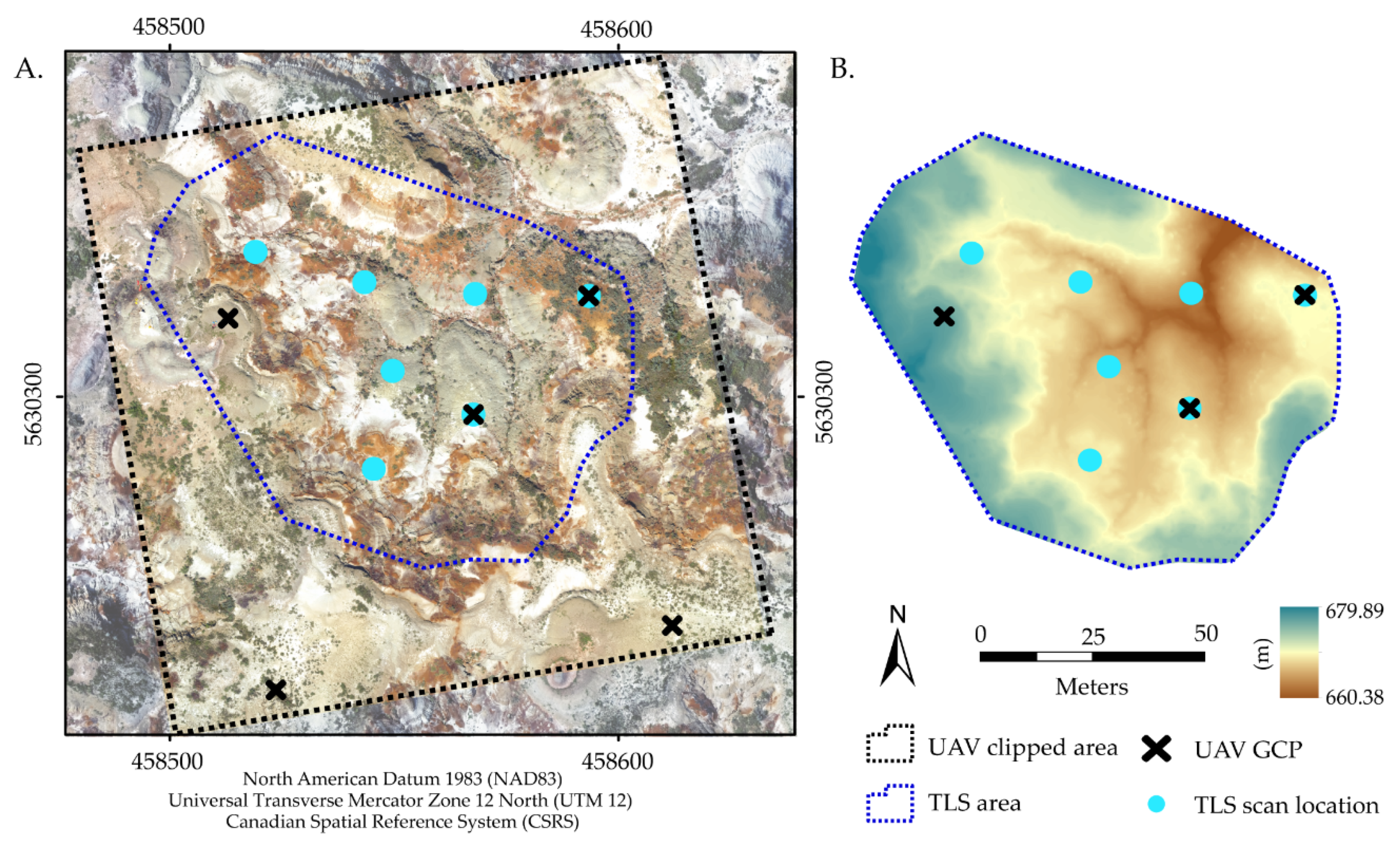
To develop the test dataset, we performed a series of UAV flights over ‘badland’ terrain associated with high drainage density. The site was located in Dinosaur Provincial Park (Figure 1A)—a UNESCO World Heritage site containing fossil-rich deposits from the Late Cretaceous Dinosaur Park and Oldman formations [68]. The incised topography, which initiated during deglaciation of the Laurentide Ice Sheet, reveals laterally continuous layers of siltstone and fine-to-medium-grained sandstone deposited by meandering channel belts [49,69,70,71]. To test UAV–SfM data collection and processing strategies, a representative section of the park was selected that contains a wide range of slope azimuths and gradients (20° mean slope), multiple changes in relief (~20 m maximum), and limited vegetation cover (Figure 1).
2.2. UAV Data Collection
UAV images were collected using a DJI Phantom 3 Professional quadcopter equipped standard with a 1/2.3” complementary metal oxide semiconductor (CMOS) sensor with 12 megapixels. The camera has a 20-mm focal length (35 mm equivalent), and a nadir image records an approximate ground footprint of 87 m × 65 m at a flying height of 50 m above ground level. This UAV records geolocation (x, y, z) to a manufacturer-stated accuracy of ±1.5 m (horizontal) and ±0.5 m (vertical) (https://www.dji.com/phantom-3-pro/info; accessed 22 January 2019), though operational conditions may be less precise [72]. The Phantom 3 Professional was selected because the camera is mounted on a three-axis gimbal that can be programmed to capture images between 0–90° and record the roll, pitch, and yaw (stated accuracy ±0.02°) relative to the flight lines of the aircraft. UAV image sets were collected over the same 125 m × 125 m footprint. UAV image blocks were pre-programmed using the freely available Pix4Dcapture application for iOS, with consistent settings for flight area, altitude (40 m above take off), and overlap (90/90 frontlap/sidelap). Pix4Dcapture also allows the user to select the camera angle for data collection, which was adjusted at 05° increments for each flight ranging from 00° (nadir) to 35° off-nadir. Higher imaging angles (e.g., 45°) were not considered in this study because SfM image-matching algorithms can be unreliable and/or camera calibration can fail with large perspective differences [6,46,73].
Each camera angle was applied for an entire image block with flight lines oriented north–south (NS), followed by a separate flight with flight lines oriented east–west (EW), creating a ‘cross-hatch’, or double-grid, image block. This resulted in 16 total image sets consisting of 231 images each. Uncontrolled variables, notably lighting conditions, were accounted for by flying during optimal (diffuse) lighting conditions whenever possible; however, natural variations and changes in cloud cover and sun angle did occur and were noted. A set of five ground control points (GCPs) were distributed throughout the field site and measured at subcentimeter precision with a Trimble R4 real-time kinematic global navigation satellite system (RTK-GNSS) and used in image processing.
2.3. UAV Processing and Scenarios
Pix4Dmapper commercial software was used to process all scenarios following steps outlined by [49,74] on a high-performance computer (Intel® Core™ i9-7900X CPU @ 3.30 GHz with 64 GB RAM and an NVIDIA GeForce GTX 1080 graphics card). Scenarios were created with variations to camera angle, changes to image overlap, different flight line directions, and combinations of nadir and oblique image sets. Image blocks collected with oblique camera angles formed convergent imaging geometry with alternating flight lines containing camera angles posed in opposing directions. To emulate lower overlap settings, images in the original image block were selectively removed so every third image and/or flight line were retained, resulting in overlap settings of 90/70 and 70/70, respectively. Image blocks composed of both NS and EW flight lines combined (NSEW) were processed for each individual camera angle (0–35°) and overlap scenario (90/90, 90/70, and 70/70).
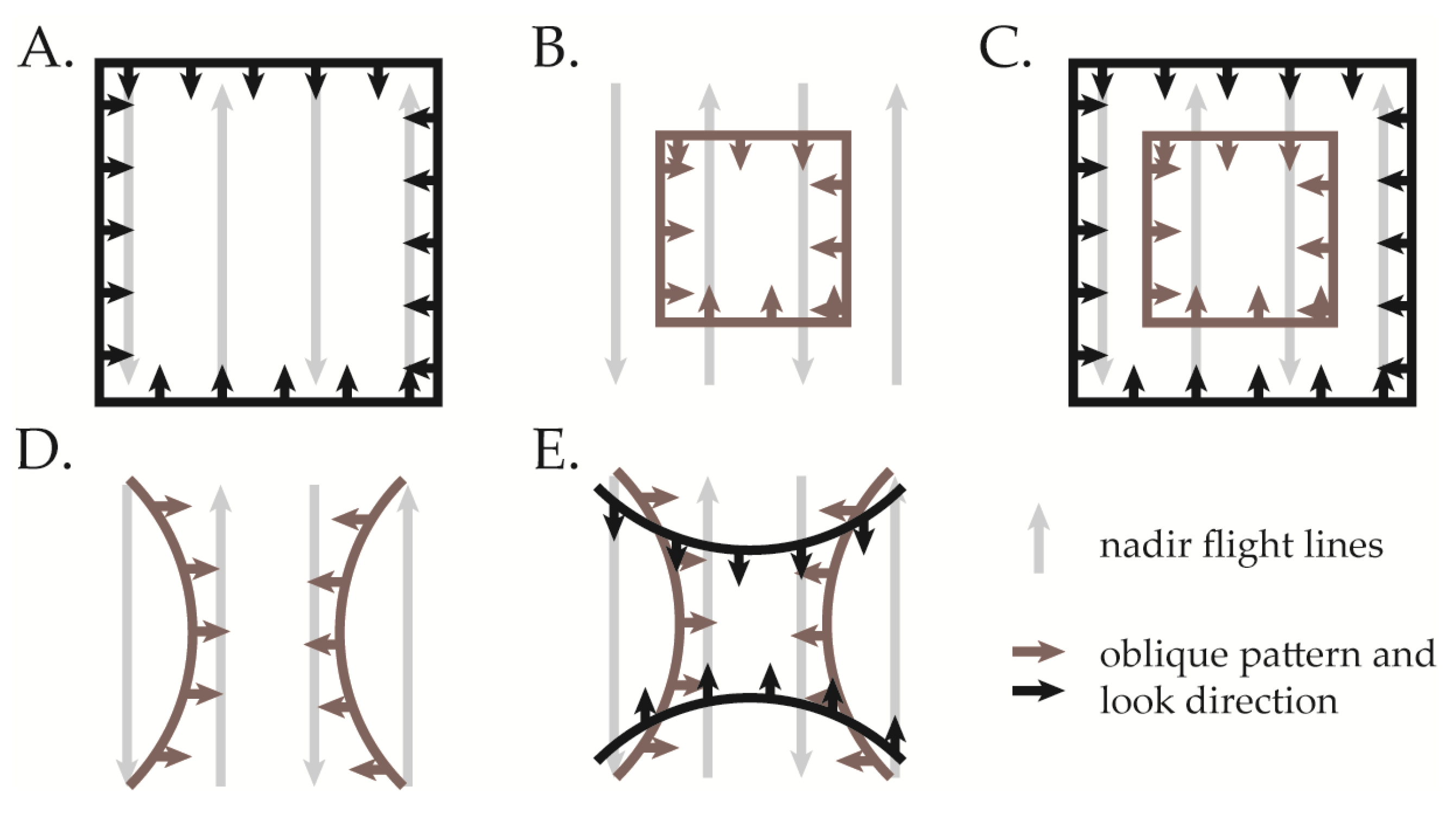
We also evaluated dataset combinations of the scenarios above based on suggestions from the literature for ideal imaging geometry and practical flight plans with common UAVs (e.g., [21]). Combinations included standard nadir-facing image blocks with various overlap and flight line settings supplemented with images selected from oblique image sets to match suggested flight patterns (Figure 2 and Table 2). Combination datasets included oblique images facing inward in (1) a box around the perimeter of nadir flight lines (Figure 2A; ‘BoxO’); (2) a box around the center of the nadir flight lines (Figure 2B; ‘BoxI’); (3) a combination of both boxes (Figure 2C; ‘BoxIO’); single convergent arcs (Figure 2D); and double convergent arcs (Figure 2E).
To ensure comparability among imaging scenarios, a consistent processing area was defined, a common GCP marking strategy used, and consistent processing settings applied. Initial image sets (90/90 overlap and both NS and EW flight lines) were imported for each camera angle and georeferenced by manually marking GCPs in every photo in which they clearly appeared. Images were then removed from the initial datasets to setup the scenarios described in the paragraphs above (Figure 2) and reprocessed using consistent processing settings for each scenario (Table 3). Processing included self-calibrating bundle block adjustment using camera internal orientation parameters: principal distance (focal length), principal point (x, y), and lens distortion terms (three radial (R1, R2, R3) and two tangential (T1, T2)) and camera external orientation parameters (location (x, y, z) and orientation (roll, pitch, yaw)). Appropriate weighting of image and GCP locations (precisions) within processing is crucial for obtaining accurate and repeatable SfM–MVS reconstructions, yet are seldom (if ever) reported in geoscience applications [13]. Precision of GCPs were defined according to instrument precisions: 0.005 and 0.010 m (horizontal and vertical) for GCPs surveyed with RTK-GNSS and a conservative 5 m and 10 m (horizontal and vertical) for UAV geotagged images.
Resulting UAV–SfM datasets had an expected ground sample distance (GSD) of 1.75–2.91 cm/pixel. Variation in GSD is caused by (1) variation of scale within individual oblique images and (2) flying height relative to underlying terrain. Pixels within an individual aerial oblique image will have a range of GSDs, such that pixels near the top of the tilted image have elongated (trapezoidal) footprints on the ground [44]. Additionally, although UAV surveys maintained a fairly consistent altitude, 40 m above takeoff from the highest local point in the field area, UAV altitude above ground level (AGL) varied up to an additional 20 m due to undulating terrain, resulting in a variation to relative flying height ranging from 40–60 m AGL. Dense point clouds produced during intermediate UAV–SfM processing steps were used for comparison (see Section 2.5 below) and had an average point spacing of 0.035–0.051 m (70/70 overlap scenarios) and 0.019–0.032 m (90/70 overlap scenarios).
A recent survey of published geoscience literature reported the ratio of root mean squared error (RMSE):viewing distance for more than 40 investigations and found a median ratio of ~1:640 [75]. Within our datasets, this would produce expected precisions ranging from 0.063–0.094 m. However, UAV–SfM combination scenarios, which include oblique images, should produce higher-precision datasets as a result of stronger image network geometry. As a result, we expect precisions to exceed this ratio and range from 0.04–0.06 m (~1:1000, precision:viewing distance), as achieved by [48].
2.4. Reference Data Acquisition and Processing
Reference data were recorded with a FARO Focus3D S120 TLS, also referred to as ground-based light detection and ranging (LiDAR). This TLS can record up to 976,000 points per second using a phase-based laser (905-nm wavelength) and has a precision of 0.01 m at a scan distance of 50 m (https://doarch332.files.wordpress.com/2013/11/e866_faro_laser_scanner_focus3d_manual_en.pdf, accessed 22 January 2019). Laser scanners are capable of recording high-precision point measurements in 3D space, but are susceptible to data gaps in locations not in direct line-of-sight of the scanner. Therefore, to avoid occlusions and data gaps around the scene, a total of six scans were acquired from various perspectives within the 7240 m2 field area. Each scan location, along with 25 checkerboard targets distributed throughout the field area, were recorded using the RTK-GNSS system described above and incorporated into scan coregistration and georeferencing processes.
Each TLS scan was individually imported, processed, and georeferenced within FARO Scene 7.1.1.81 software. Initial scan locations (applied from RTK-GNSS) and orientation information (from integrated sensors) were refined by manual identification of at least four checkerboard targets appearing in multiple TLS scans. Fine registration was then performed using cloud-to-cloud registration of all TLS datasets and then merged into a single point cloud. A final alignment and optimization was performed to fit the merged point cloud to RTK-GNSS control points, resulting in a final registration error of 0.013 m, approximately half the size of the expected GSD within UAV–SfM models. Points were filtered to remove any colocated points within 0.002 m of another point, resulting in a merged point cloud of 231 million points. This point cloud was filtered to remove vegetation using the CANUPO plugin [76] in the open source CloudCompare software [77]. Vegetation was removed due to the added uncertainty in point cloud datasets and issues known in UAV–SfM reconstruction [78,79], creating a final reference dataset of 186 million points with an average point spacing of 0.004 m.
2.5. Point Cloud Accuracy
Several methods have been used to validate SfM–MVS accuracy in the geosciences, with point-based metrics, such as RMSE and mean absolute error (MAE), being the most common. Though point measurements can be extremely precise, spatial variability of errors may remain imperceptible without sufficient number and distribution of validation points [75]. Surface-to-surface comparisons have been used to document the changes between two continuous surfaces, such as digital elevation models (DEMs). DEMs are 2.5D interpolations with a single elevation (z) attribute for each planar (x, y) location that may reveal spatial variability, but can also result in overgeneralization and degradation of highly three-dimensional landscapes [49,54,62,80].
To assess the accuracy of the various UAV–SfM processing scenarios in our topographically complex field area, we use the freely available Multiscale Model to Model Cloud Comparison (M3C2) plugin for open-source CloudCompare software [80]. M3C2 calculates local differences between two point clouds relative to local surface normal orientation and point cloud roughness. Normal orientations are locally calculated by averaging points within a user-defined radius (D/2) in the reference point cloud (PC1). A cylinder with user-defined radius (d/2) is then projected along the normal direction (N) to specify the search space on the target point cloud (PC2). The algorithm then calculates the average position of points within the cylinder for both PC1 and PC2 and calculates the local difference between the two positions. To limit the influence of point cloud roughness on difference calculations, D was defined as 0.1 m, following recommendations to define D as >20 to 25 times the average local roughness [80] and methods in [81]. A subsample of the TLS reference cloud was created using 10% of the point cloud and used to compare all UAV–SfM point clouds with a consistent reference dataset. M3C2 distances between point clouds were calculated between the TLS reference point cloud (0.004 m average point spacing) and UAV–SfM point clouds (0.019–0.051 m average point spacing). Calculations were carried out by differencing UAV–SfM point clouds from the TLS reference point cloud, with negative distances indicating that the TLS surface was above the UAV–SfM surface and positive values signifying that the UAV–SfM surface was above the reference TLS surface.
3. Results
3.1. Single Camera Angle and Single Flight Direction
Images collected along a single flight line orientation (NS or EW) generally resulted in inconsistent coverage, especially along the perimeter of the field area, and substantial data gaps (up to 14 × 8 m) within point clouds. Data gaps due to insufficient coverage typically occurred along steep slopes in different locations throughout the field area, dependent on the flight line orientation and camera tilt angle during acquisition. Due to incomplete coverage and shifting data gap locations, single flight line datasets were considered unsuitable for comparison and removed from further analysis. However, datasets that combined NS and EW flight lines into ‘cross-hatch’ (NSEW) datasets and/or included supplemental oblique images in various patterns (Figure 2) resulted in reduced data gaps. Readers should note that data gaps occurring in the same locations of the remaining analyses were the expected result of vegetation removal from the TLS reference point cloud (Section 2.4).
3.2. Single Camera Angle and Cross-Hatch Flight Lines
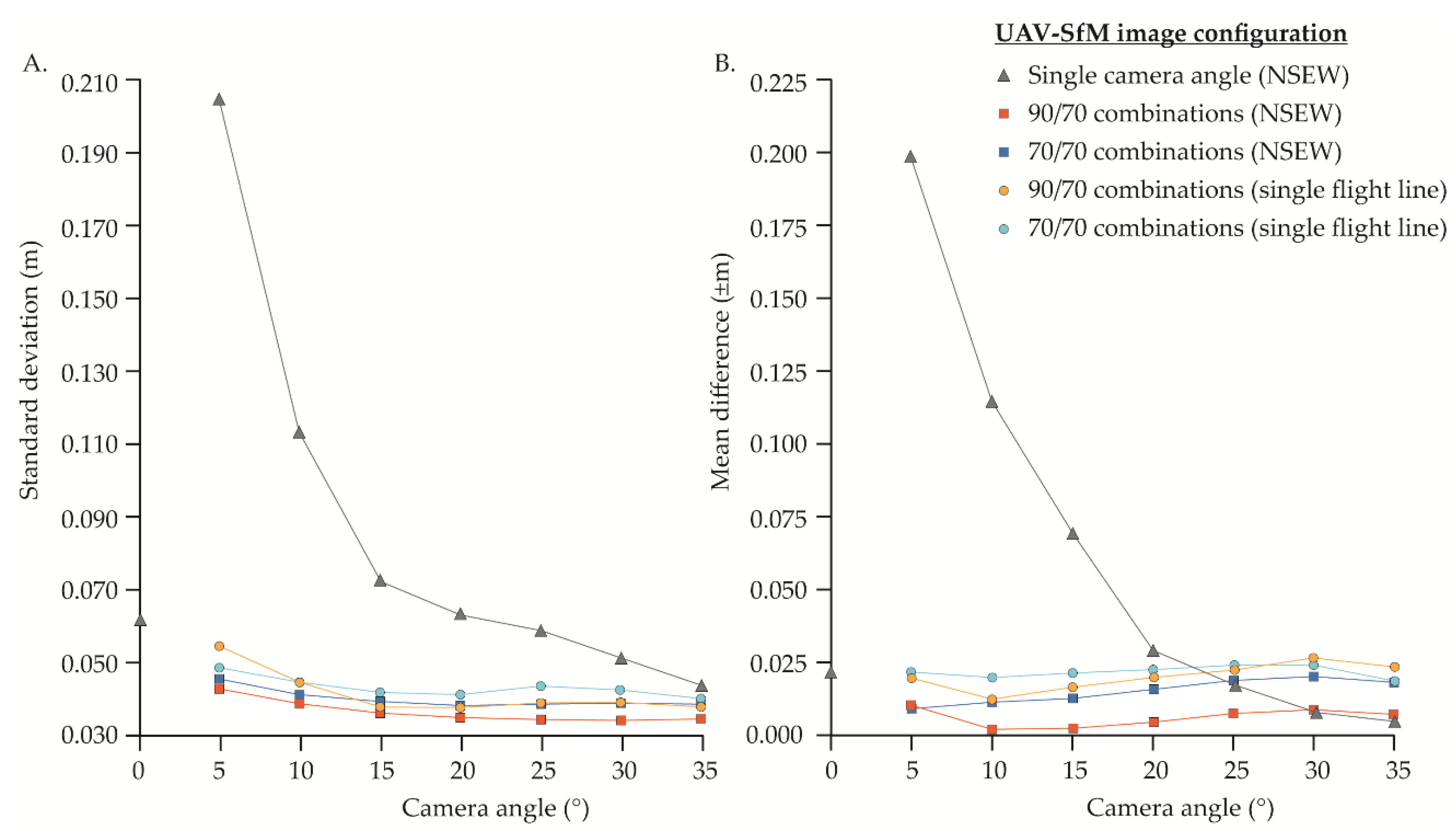
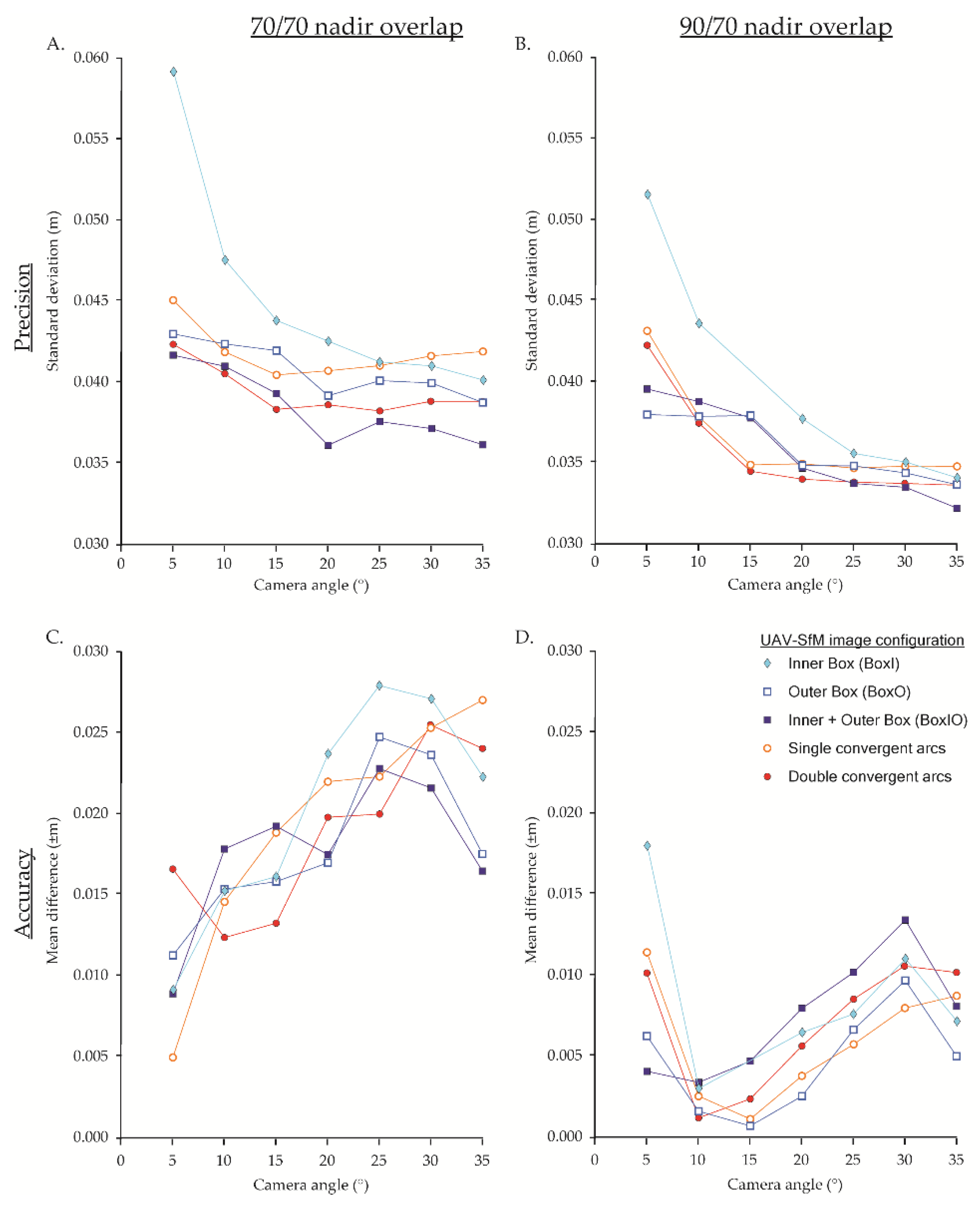
Image blocks collected with a single camera angle and cross-hatch flight lines produced complete datasets with smaller data gaps for all overlap scenarios (70/70, 90/70, and 90/90). Datasets collected with a single camera angle always resulted in higher standard deviations (lower precision) of M3C2 distance measurements between UAV–SfM and TLS models than combination datasets (Figure 3A) and usually had means further from 0 (lower accuracy) than combination datasets (Figure 3B). Single-angle datasets with high tilt angles (25–35°) had mean values similar to or smaller than combination datasets (Figure 3B). High tilt angles usually resulted in standard deviations lower than nadir-only datasets and higher than combination datasets (Figure 3A).
Within single-angle datasets (Figure 4), overlap did not have a direct relationship with precision (i.e., increasing overlap did not always increase precision). Increasing overlap from 70/70 to 90/70 resulted in better precision for most datasets, but increasing from 90/70 to 90/90 resulted in lower precisions, except for the nadir and 05° datasets (Figure 4A). Increasing overlap for single-angle datasets had a direct relationship with mean values (Figure 4B); lower overlap (70/70) resulted in smaller mean values, while high overlap (90/70 and 90/90) produced larger mean values for all camera angles. Regardless of camera angle, high-overlap scenarios consistently resulted in higher point counts. Among datasets with similar overlap, increasing camera angle always resulted in lower standard deviations and smaller mean values, with the exception of nadir-only image blocks (Figure 4). Nadir-only datasets had lower standard deviations and smaller means than all other single-angle datasets, except for high oblique angles (30–35°), which outperformed all nadir-only datasets regardless of overlap (Figure 4). Increasing camera angle typically resulted in decreasing point counts, with nadir-only image blocks containing the most points among similar overlap scenarios.
Although nadir-only datasets generally had higher point counts, higher precision, and mean values closer to 0, the spatial distribution of difference values reveals a systematic pattern of errors (Figure 5). This pattern represents UAV–SfM underestimation of height values of high elevation points (near the perimeter of the scene) and overestimation of low elevation points (near the center of the scene) in nadir-only image blocks. All single-angle oblique datasets may also contain a systematic error pattern (Figure 6). Most evident in lower oblique angles (05–15°), this pattern contains differences in which lows are too low and highs are too high.
3.3. Nadir Image Blocks (NSEW) Supplemented with Oblique Images
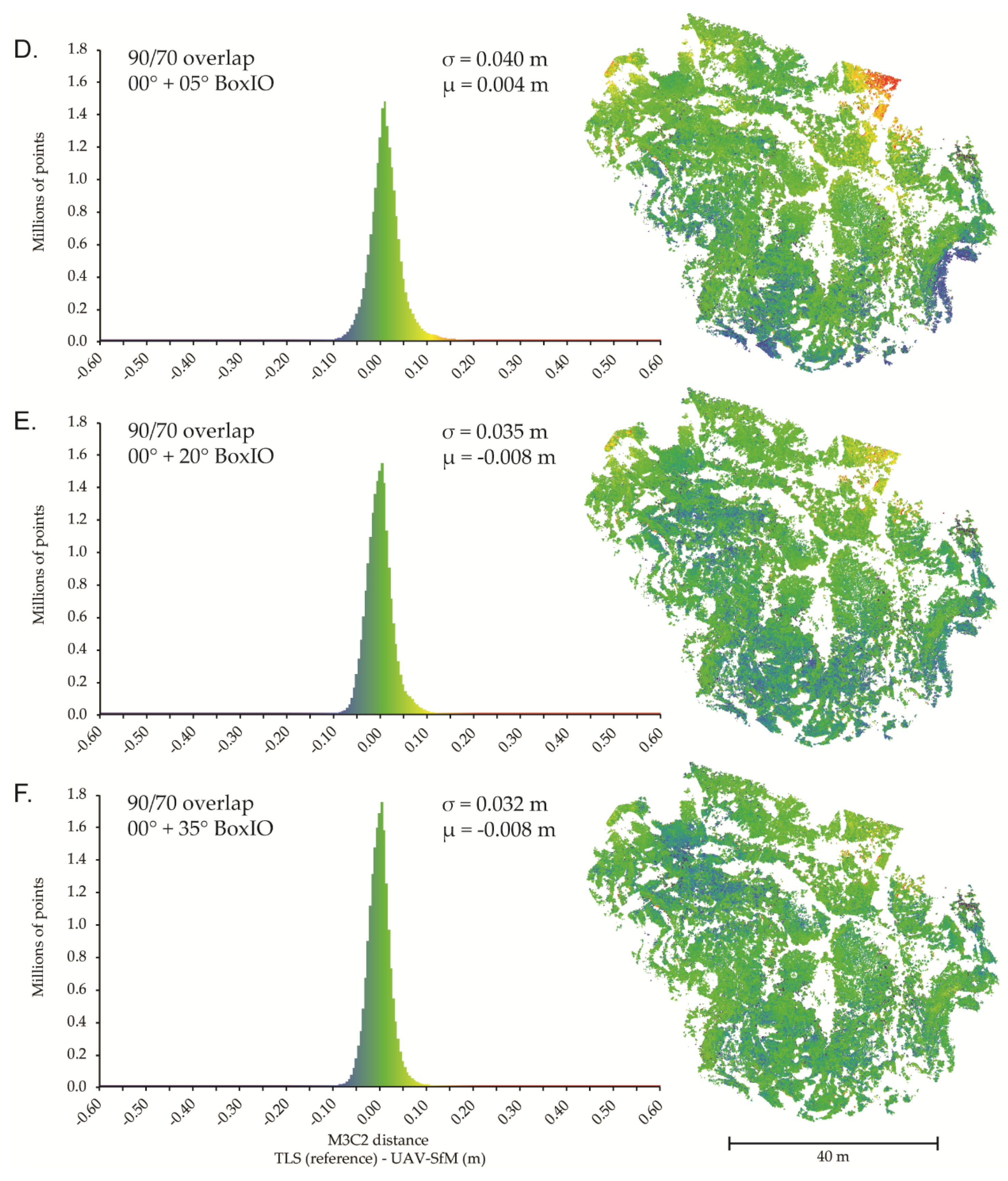
Inclusion of oblique images into nadir image blocks with cross-hatch (NSEW) flight lines diminished the systematic error present in nadir-only image blocks, regardless of oblique image angle and flight pattern (Figure 7). In each oblique combination scenario, precision and accuracy were better than or equal to any nadir-only dataset (Figure 3). Datasets incorporating oblique combinations had a maximum difference in precision of 0.027 m and absolute difference in accuracy of ±0.028 m. Among combination datasets, high-overlap scenarios typically had lower standard deviations than lower-overlap scenarios, regardless of oblique flight pattern (Figure 8A,B). Combinations that included high angles had smaller standard deviations in both 90/70 and 70/70 overlap scenarios. Combinations with supplemental oblique camera angles between 10–15° had the smallest means, while 25–30° were consistently further from 0 (Figure 8C,D). Nadir image blocks supplemented with oblique images always resulted in more points than any single-angle image block with similar overlap. Point increases for combination datasets (relative to nadir-only datasets) were typically greatest for oblique angles of 15° and smallest for angles of 35° (low-overlap scenario) or 5–10° (high-overlap scenario).
3.4. Nadir Image Blocks (Single Flight Line) Supplemented with Oblique Images
Single flight direction (NS or EW) datasets supplemented with oblique images produced complete coverage and reduced data gaps compared to those without oblique images. Single flight direction datasets supplemented with oblique images had lower standard deviations than all nadir-only and most single oblique camera angle datasets (Figure 3A). Single flight line combinations generally had slightly lower precision (Figure 3A) and lower accuracy (Figure 3B) than cross-hatched flight line combinations with similar overlap. For oblique angles 15–35°, high-overlap (90/70) single flight line combinations had similar standard deviations to low-overlap (70/70) cross-hatched flight line combinations.
3.5. Combination Datasets—Flight Pattern
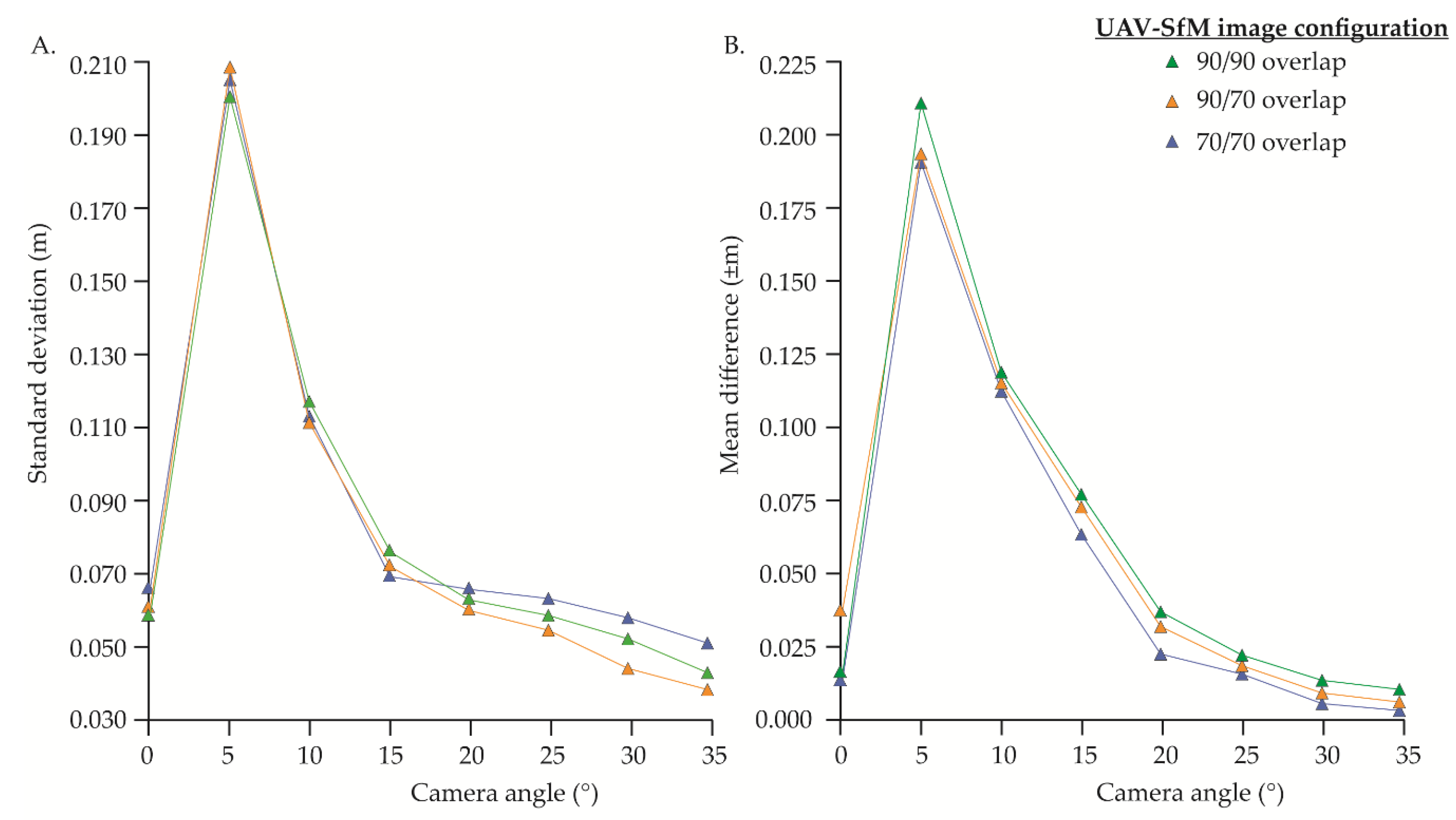
Image configuration of supplemental oblique images had some effect on UAV–SfM dataset precision and accuracy (Figure 8). The inner box (BoxI) and single convergent arc patterns (Figure 2B,D, respectively) generally resulted in the highest standard deviations and means farthest from 0 compared to datasets with similar overlap and camera angle. Outer box (BoxO), inner/outer box (BoxIO), and double convergent arc patterns (Figure 2A,C,E) usually resulted in highest precisions; double convergent arcs were more effective for low angles (10–15°), while box patterns were slightly more effective for high angles (25–35°), particularly for the 70/70 overlap scenario (Figure 8A). Mean difference values were also affected by different oblique image configurations, although results were less consistent. Oblique flight patterns resulting in small means (closest to 0 m) varied considerably within the 70/70 overlap scenario (Figure 8C), while the 90/70 scenario typically had smallest means for single convergent arcs and BoxO patterns and largest mean values for BoxIO and double convergent arc patterns (Figure 8D).
4. Discussion
Our results confirm the presence of systematic vertical deformations (i.e., ‘dome effect’ [21]) within UAV–SfM datasets processed from parallel-axis (nadir) image blocks and further verify effective data acquisition strategies for mitigating such errors. We build upon recommended image acquisition strategies (e.g., [21]) by evaluating more than 150 scenarios and quantifying differences among various oblique imaging angles. Results indicate that imaging angle has a profound impact on accuracy and precision for data acquisition with a single camera angle (Figure 6) in topographically complex scenes. Combination scenarios generally revealed consistent improvements relative to nadir-only image blocks, regardless of oblique imaging angle and pattern. However, differences among oblique imaging patterns and camera angles for combination datasets only revealed subtle differences that do not decisively determine an optimal configuration for UAV–SfM applications in complex topographic landscapes.
Results are based on M3C2 distances, which are calculated in the direction of surface normals of the reference point cloud, rather than strictly vertical distances. Relating results and GCP residuals to the topography of the field site (Figure 1B) suggests that vertical error is more prevalent than horizontal. Differences between the TLS reference dataset and UAV–SfM datasets could be attributed to inconsistencies/deformation of reconstructed surface shape (relative accuracy), georeferencing errors (absolute accuracy), or a combination of both. Within this investigation, TLS data was considered as the reference dataset because of its superior precision and a final georegistration error of 0.013 m. UAV–SfM datasets had resulting precisions more than a magnitude higher than the TLS, but GCP residuals in UAV–SfM datasets were generally comparable. This suggests that deviations between the TLS reference dataset and various UAV–SfM scenarios were primarily a result of differences in surface shape in the dense point clouds. Some datasets, however, exhibited large inconsistencies in both georeferencing and surface shape, most notably 05–10° (Figure 6B,C), which had vertical RMSE values up to 0.13 m.
4.1. Nadir-Only Image Blocks
Nadir-only image blocks resulted in systematic ‘dome’ errors that can be attributed to inaccurate estimation of radial lens distortion from self-calibration of the relatively unstable, consumer-grade digital camera used on the UAV [21]. Although this has been well-documented in the literature, nadir-only image blocks remain widespread UAV–SfM data collection strategies. Applications in the geosciences have often accounted for systematic doming by using well-dispersed and high-precision control points. However, as previously stated [21] and documented ([62], Figure 6A) and further confirmed by our results (Figure 5), use of GCPs does not guarantee that systematic vertical doming errors will be reduced to negligible levels.
Some authors have suggested that increasing overlap or including cross-strips in airborne image blocks can help reduce systematic errors due to higher redundancy [42,82]. Others have noted that increased overlap results in shorter baselines (distance between adjacent photos) and subsequently narrower angles of ray convergence, ultimately subjecting calculated object space locations to errors, especially in depth/height [53,62]. Our results suggest that increasing overlap may slightly lower the standard deviation in nadir-only scenarios (Figure 4 and Figure 5), but an increase in the number of images does not linearly increase accuracy [83] and systematic doming errors remained clearly visible, regardless of overlap (Figure 5).
4.2. Single Oblique Camera Angle Image Blocks
Collecting image blocks with a single off-nadir camera angle has been recommended as an effective means for reducing systematic deformation [21]; however, recommendations within the literature are not consistent (Table 1). Our results quantify the effects of different imaging angles on point cloud accuracy in high-relief landscapes. Lower oblique image angles between 0–15° (Figure 6B–D) clearly reveal a systematic error that also corresponds to lower precisions and means further from 0 m. However, deformation appears as a concave ‘bowl’ shape rather than a convex dome. Large GCP residuals in these datasets appear to contribute to the large discrepancies with the TLS reference through large mean offsets (Figure 6B–D); however, the wide range of values suggests that surface reconstruction is also contributing to errors relative to the reference data.
Based on these results, users should be cautioned against collecting full image sets at very low-oblique angles to the object of interest. Specifically, this may pertain to applications flown with a manual ‘free flight’ mode in which camera angles may be close, but not directly orthogonal to the surface. Additionally, data quality in manual flight modes is inherently reliant on the remote piloting skills of the operator and can often result in notable data gaps, especially in complex landscapes [22]. Increasing camera angle further off-nadir appears to mitigate the systematic bowl effect and increase precision and accuracy (Figure 6E–H). Precisions achieved with these single camera angle (20–35°) image blocks are similar to the 1:1000 ratio attained by [48], while lower oblique camera angles fail to achieve the ~1:640 ratio realized in [75]. It is worth considering that systematic errors may still be occurring outside our assessment area, but this is subject to future research considerations. Good GCP distribution appears specifically necessary for these single camera angle datasets, as the most prevalent errors consistently occur in the N–NW areas (Figure 6), outside the constraints of GCPs.
Collection of image blocks with single off-nadir camera angles is not a common practice in UAV or piloted aircraft image collection. These datasets resemble multicam image sets (one nadir and four 45° off-nadir sensors), which are growing in popularity in both conventional and SfM communities for mapping complex 3D scenes, such as cities. Multicams with oblique sensors are not yet widely available for UAVs and research on the capabilities of such imaging geometries is still developing. However, our results suggest that SfM software is capable of processing off-nadir image sets and may produce more optimal results than nadir-only image blocks.
4.3. Combination Datasets
Our findings further confirm that supplementing parallel-axis (nadir) image blocks with oblique images reduces or eliminates systematic dome errors in UAV–SfM datasets, regardless of overlap, camera angle, and oblique image configuration (Figure 7). Combination datasets always resulted in more points produced, lower standard deviations (higher precision), and had comparable or better mean values relative to nadir-only datasets (Figure 3). Nadir-only datasets consistently had precision:viewing distance ratios of ~1:1000, while nadir image blocks supplemented with oblique images produced ratios ~1:1500, regardless of oblique imaging pattern and overlap. Production of more points can be simply explained by a higher number of input images allowing for the calculation of more matching points within the final SfM model. Additionally, oblique images may obtain a better viewing angle of steep slopes that are not easily visible in nadir images, thus producing more potential matching points in both SfM and MVS steps. This is consistent with Vacca et al. [32], who found tie point matching to be quite successful between nadir and oblique (45°) images.
Increasing camera tilt angle in combination datasets generally improved precision, but also resulted in lower accuracy (Figure 8). Lower oblique images (05–10°) have a similar perspective to nadir images and therefore may not provide substantial benefits for self-calibration due to narrow angles of intersection (parallactic angles). In contrast, inclusion of higher oblique camera angles resulted in larger parallactic angles (closer to 90°) known to be beneficial for self-calibration [20,55,83]. Regardless of oblique tilt angle, higher-overlap scenarios typically resulted in higher precision and accuracy (Figure 3), which is likely a result of greater redundancy (i.e., more object points observed in more images). This is consistent with other studies [42,67,84] and the direct relationship between overlap and precision of nadir-only image blocks within this study (Figure 4A). In combination scenarios, accuracy may be adversely affected by the proportion of oblique images relative to nadir images used in SfM processing. Suggestions from the literature indicate that oblique images should constitute ~10% of an image block [54]. Our results seem to show agreement with this suggestion, with higher-overlap image blocks (6.7–14.4% oblique images) typically producing better results than the lower-overlap scenarios (up to 33.3% oblique images); however, a more rigorous investigation on the impact of oblique image proportions within a given image block is warranted.
Imaging pattern of oblique images also appears to have an influence on precision and accuracy. Oblique image patterns with more images (e.g., BoxIO and double convergent arcs) consistently produced datasets with the highest precision (Figure 8A,B), but lowest accuracy (Figure 8C,D), especially in the higher overlap scenario. Higher precision and lowest accuracy may again be related to the proportion of oblique images, but we suspect that image locations also have a strong influence. For example, a 30° oblique image in BoxI may record ~40% of the field area, leaving more than half of the image frame unused in generating tie points, and as a result, tie point matches are concentrated in only a portion of the image frame, which is considered less than ideal for self-calibrating bundle adjustment [50]. Conversely, a 30° oblique image in the BoxO pattern captures ~65% of the scene, and consequently, has the potential to produce more tie point matches and have a greater influence on camera calibration.
4.4. Cameras and Calibration
Low-cost sensors commonly used in UAV applications, such as the one used in this study, are relatively unstable [9,57] and common SfM processing solutions may give a false sense of quality while errors propagate into the final model [55,56], as demonstrated in this investigation. Previous studies have thoroughly demonstrated the benefits of oblique images for camera calibration [21,50]; however, obtaining an optimal image network for both calibration purposes and scene reconstruction is not always straightforward [60]. Self-calibration can be performed prior to data acquisition (precalibration) or calculated simultaneously with 3D object space point coordinates (‘on-the-job’). Remondino et al. [85] suggested that a separation of calibration and scene reconstruction is preferable, but this assumes similar conditions between calibration and scene acquisition. In contrast, a direct comparison of pre- and ‘on-the-job’ self-calibration of UAV image blocks has yielded similar results [52]. Within this investigation, ‘on-the-job’ self-calibration with combination scenarios that included oblique images provided satisfactory results and improved precision relative to single camera angle datasets. Due to practical and logistical concerns, ‘on-the-job’ self-calibration is likely to remain the most applied method within geoscience research [21,86].
Although cameras are continuously being produced in smaller sizes with improved resolution and stability, an accurate camera calibration will always be essential for reliable photogrammetric measurements. Many UAVs have the flexibility to facilitate improved calibration by collecting airborne images with varying orientations (e.g., multirotor platforms with gimbaled cameras, senseFly S.O.D.A. 3D (https://www.sensefly.com/camera/sensefly-s-o-d-a-3d/; accessed 22 January 2019)). Therefore, we strongly urge practitioners employing UAV–SfM (and ground-based SfM) methods to implement data collection strategies that consider the well-established ‘rules’ of self-calibration (Section 1), specifically items (1–3).
4.5. GCPs
Precise and well-distributed GCPs are important for obtaining accurate and reliable UAV–SfM models; GCPs define the absolute orientation and scale within an external coordinate system and provide constraints within the bundle adjustment [13,21,67,83]. Our results show that GCPs are especially important for single camera angle datasets. The zone of weakness occurring in the NW corner of Figure 6E–H (peripheral to all GCPs) is a textbook example of the deficiencies that can result outside the surface constrained by GCPs. At a minimum, for accurate results, GCPs should be placed around the perimeter of the field area of interest [50]; however, feasibility and accessibility may hinder GCP planning.
As a result, logistical and practical motivations are driving interests in a number of applications (e.g., geologic mapping) to reduce or completely omit the use of GCPs. Incorporation of oblique images should reduce the need for a dense network of precise GCPs [13], particularly for constraining the bundle adjustment. Harwin et al. [52] found that with fewer GCPs or lower precision measurements, oblique images were especially effective for improving camera calibration and resulting 3D model accuracy; however, more GCPs should be preferred. Combination datasets in this investigation (Figure 7) appear to reduce GCP requirements; in the NW zone of weakness (outside the GCP area), errors were reduced by nearly 50% in combination datasets (most notably in 90/70 overlap) relative to single camera angle datasets. Although oblique images may reduce the need for GCPs, some control measurements are still recommended to add external constraints to the bundle adjustment along with providing absolute orientation.
Recent advances in UAV onboard orientation sensors (e.g., real-time kinematic global navigation satellite system, RTK-GNSS), provide an attractive solution for direct georeferencing (DG) without the need for GCPs. Although DG UAV–SfM has shown comparable planar (x, y) accuracy to surveys incorporating GCPs, vertical accuracy may still be up to a magnitude poorer [86,87]. Through the addition of oblique images, accuracy and precision of DG UAV–SfM could be nearly commensurate with surveys incorporating GCPs [54]. However, this topic requires further investigation and we expect that higher-grade inertial measurement units (IMUs) may be required to provide accurate angular camera orientation (yaw, pitch, and roll) within the solution, and that weighting capabilities for angular orientation will also need to be available within processing software.
4.6. Software and Settings
Readers should be cautioned that oblique images may create complications within certain SfM-MVS processing software. A limitation of this study is the evaluation of a single software package, Pix4Dmapper, an established commercial SfM solution that has consistently demonstrated reliability in processing oblique images (e.g., [32,43,88]). A list of additional software packages that have been successfully used in processing oblique images can be found in Verykokou and Ioannidis [30]. Although many commercial photogrammetric software suites have optimized aerial triangulation of oblique images [88], most retain proprietary details and continuously modify algorithms to improve efficiency and precision. Software packages may offer users limited options for processing that can alter image matching strategies; however, the use of a matching strategy that is inappropriate with the image set can result in failure during processing.
5. Conclusions
UAV–SfM workflows have demonstrated the ability to map extensive 2D planes and model isolated 3D objects. Complex scenes with high-relief and intricate geometric morphology, however, require deeper consideration of imaging strategy to maintain detail and accuracy in planar (x, y) and vertical (z) dimensions. Within topographically complex scenes, image sets collected with a single camera angle are unlikely to produce complete datasets and are prone to higher levels of deformation along steep slopes. Parallel-axis image sets (i.e., nadir image blocks) are susceptible to systematic ‘dome’ deformation, even with the use of survey-grade control points within high-relief scenes. As suggested by several authors, our results confirm that supplementing nadir image blocks with oblique images consistently mitigates these systematic error patterns within complex topography. Results from more than 150 scenarios with various combinations of overlap and imaging angles provide quantitative evidence of increased precision, higher accuracy, and reduced data gaps within combination datasets. Based on our results and the existing literature, we provide the following recommendations for improving UAV–SfM surveys in high-relief terrain. These recommendations should be equally adaptable for SfM data acquisition in alternative scenarios (e.g., vertical façades from UAV or ground-based imaging):
- Combination datasets (i.e., nadir image block supplemented with off-nadir images) are preferred over image sets collected using a single camera angle.
- Higher overlap is preferred for combination datasets.
- Higher camera tilt angles (15–35°) in combination datasets generally increase precision, but may have an adverse effect on accuracy.
- Single-angle image sets at higher-oblique angles (30–35°) can produce reliable results if combination datasets are not possible. However, single-angle image sets collected at lower angles may be more volatile and can result in large systematic errors. This should prove cautionary for image sets collected at near orthogonal angles using manual ‘free flight’ modes.
Author Contributions
This investigation was conceptualized and designed by P.R.N. under the supervision of C.H.H. Datasets were collected with assistance (see Acknowledgments), processed, and analyzed by P.R.N. Original manuscript preparation was conducted by P.R.N. with input on analysis and content review and editing by C.H.H.
Funding
This research was supported by the Natural Sciences and Engineering Research Council of Canada (NSERC). P.R.N. was supported by the University of Calgary Eyes High Doctoral Recruitment Scholarship.
Acknowledgments
The authors would like to thank Dinosaur Provincial Park for continued research access (Research Permit # 17-146) and land access from John Genovese and Lloyd Xi. We would also like to thank Paul Durkin and Maja Kucharczyk for their field assistance in obtaining the data used for analysis in this manuscript. We thank the Associate Editor and three anonymous reviewers for constructive comments that have contributed to the improvement of this manuscript.
Conflicts of Interest
The authors declare no conflict of interest.
References
- Harwin, S.; Lucieer, A. Assessing the accuracy of georeferenced point clouds produced via multi-view stereopsis from Unmanned Aerial Vehicle (UAV) imagery. Remote Sens. 2012, 4, 1573–1599. [Google Scholar] [CrossRef]
- Hugenholtz, C.H.; Moorman, B.J.; Riddell, K.; Whitehead, K. Small unmanned aircraft systems for remote sensing and earth science research. Eos Trans. Am. Geophys. Union 2012, 93, 236. [Google Scholar] [CrossRef]
- Niethammer, U.; James, M.R.; Rothmund, S.; Travelletti, J.; Joswig, M. UAV-based remote sensing of the Super-Sauze landslide: Evaluation. Eng. Geol. 2012, 128, 2–11. [Google Scholar] [CrossRef]
- Westoby, M.J.; Brasington, J.; Glasser, N.F.; Hambrey, M.J.; Reynolds, J.M. “Structure-from-Motion” photogrammetry: A low-cost, effective tool for geoscience applications. Geomorphology 2012, 179, 300–314. [Google Scholar] [CrossRef]
- Fonstad, M.A.; Dietrich, J.T.; Courville, B.C.; Jensen, J.L.R.; Carbonneau, P.E. Topographic structure from motion: A new development in photogrammetric measurement. Earth Surf. Process. Landf. 2013, 38, 421–430. [Google Scholar] [CrossRef]
- Bemis, S.P.; Micklethwaite, S.; Turner, D.; James, M.R.; Akciz, S.; Thiele, S.T.; Bangash, H.A. Ground-based and UAV-Based photogrammetry: A multi-scale, high-resolution mapping tool for structural geology and paleoseismology. J. Struct. Geol. 2014, 69, 163–178. [Google Scholar] [CrossRef]
- Whitehead, K.; Hugenholtz, C.H.; Myshak, S.; Brown, O.W.; LeClair, A.; Tamminga, A.D.; Barchyn, T.E.; Moorman, B.J.; Eaton, B.C. Remote sensing of the environment with small unmanned aircraft systems (UASs), part 2: Scientific and commercial applications 1. J. Unmanned Veh. Syst. 2014, 2, 86–102. [Google Scholar] [CrossRef]
- Smith, M.W.; Carrivick, J.L.; Quincey, D.J. Structure from motion photogrammetry in physical geography. Prog. Phys. Geogr. 2015, 40, 247–275. [Google Scholar] [CrossRef] [Green Version]
- Carrivick, J.L.; Smith, M.W.; Quincey, D.J. Structure from Motion in the Geosciences; Wiley-Blackwell: Oxford, UK, 2016. [Google Scholar]
- Chesley, J.T.T.; Leier, A.L.L.; White, S.; Torres, R. Using unmanned aerial vehicles and structure-from-motion photogrammetry to characterize sedimentary outcrops: An example from the Morrison Formation, Utah, USA. Sediment. Geol. 2017, 354, 1–8. [Google Scholar] [CrossRef]
- Colomina, I.; Molina, P. Unmanned aerial systems for photogrammetry and remote sensing: A review. ISPRS J. Photogramm. Remote Sens. 2014, 92, 79–97. [Google Scholar] [CrossRef] [Green Version]
- Toth, C.; Jóźków, G. Remote sensing platforms and sensors: A survey. ISPRS J. Photogramm. Remote Sens. 2016, 115, 22–36. [Google Scholar] [CrossRef]
- James, M.R.; Robson, S.; D’Oleire-Oltmanns, S.; Niethammer, U. Optimising UAV topographic surveys processed with structure-from-motion: Ground control quality, quantity and bundle adjustment. Geomorphology 2017, 280, 51–66. [Google Scholar] [CrossRef]
- Zahm, C.; Lambert, J.; Kerans, C. Use of unmanned aerial vehicles (UAVs) to create digital outcrop models: An example from the Cretaceous Cow Creek Formation, Central Texas. GCAGS J. 2016, 5, 180–188. [Google Scholar]
- Carvajal-Ramírez, F.; Agüera-Vega, F.; Martínez-Carricondo, P.J. Effects of image orientation and ground control points distribution on unmanned aerial vehicle photogrammetry projects on a road cut slope. J. Appl. Remote Sens. 2016, 10, 034004. [Google Scholar] [CrossRef]
- Thoeni, K.; Guccione, D.E.; Santise, M.; Giacomini, A.; Roncella, R.; Forlani, G. The potential of low-cost rpas for multi-view reconstruction of sub-vertical rock faces. Int. Arch. Photogramm. Remote Sens. Spat. Inf. Sci. ISPRS Arch. 2016, 41, 909–916. [Google Scholar] [CrossRef]
- Nieminski, N.M.; Graham, S.A. Modeling Stratigraphic Architecture Using Small Unmanned Aerial Vehicles and Photogrammetry: Examples From the Miocene East Coast Basin, New Zealand. J. Sediment. Res. 2017, 87, 126–132. [Google Scholar] [CrossRef]
- Agüera-Vega, F.; Carvajal-Ramírez, F.; Martínez-Carricondo, P.J.; Sánchez-Hermosilla López, J.; Mesas-Carrascosa, F.J.; García-Ferrer, A.; Pérez-Porras, F.J. Reconstruction of extreme topography from UAV structure from motion photogrammetry. Meas. J. Int. Meas. Confed. 2018, 121, 127–138. [Google Scholar] [CrossRef]
- Mikhail, E.M.; Bethel, J.S.; McGlone, J.C. Introduction to Modern Photogrammetry; John Wiley & Sons, Inc.: New York, NY, USA, 2001. [Google Scholar]
- Wolf, P.R.; Dewitt, B.A.; Wilkinson, B.E. Elements of Photogrammetry with Application in GIS, 4th ed.; McGraw-Hill Education: Maidenhead, UK, 2014. [Google Scholar]
- James, M.R.; Robson, S. Mitigating systematic error in topographic models derived from UAV and ground-based image networks. Earth Surf. Process. Landforms 2014, 39, 1413–1420. [Google Scholar] [CrossRef] [Green Version]
- Martin, R.; Rojas, I.; Franke, K.W.; Hedengren, J.D. Evolutionary View Planning for Optimized UAV Terrain Modeling in a Simulated Environment. Remote Sens. 2016, 8, 26. [Google Scholar] [CrossRef]
- Dueholm, K.S.; Olsen, T. Reservoir analog studies using multimodel photogrammetry: A new tool for the petroleum industry. Am. Assoc. Pet. Geol. Bull. 1993, 77, 2023–2031. [Google Scholar] [CrossRef]
- Rittersbacher, A.; Buckley, S.J.; Howell, J.A.; Hampson, G.J.; Vallet, J. Helicopter-based laser scanning: A method for quantitative analysis of large-scale sedimentary architecture. Geol. Soc. London, Spec. Publ. 2014, 387, 185–202. [Google Scholar] [CrossRef]
- Rossi, P.; Mancini, F.; Dubbini, M.; Mazzone, F.; Capra, A. Combining nadir and oblique UAV imagery to reconstruct quarry topography: Methodology and feasibility analysis. Eur. J. Remote Sens. 2017, 50, 211–221. [Google Scholar] [CrossRef]
- O’Connor, J.; Smith, M.J.; James, M.R. Cameras and settings for aerial surveys in the geosciences. Prog. Phys. Geogr. 2017, 41, 325–344. [Google Scholar] [CrossRef]
- Vollgger, S.A.; Cruden, A.R. Mapping folds and fractures in basement and cover rocks using UAV photogrammetry, Cape Liptrap and Cape Paterson, Victoria, Australia. J. Struct. Geol. 2016, 85, 168–187. [Google Scholar] [CrossRef]
- Pavlis, T.L.; Mason, K.A. The New World of 3D Geologic Mapping. GSA Today 2017, 4–10. [Google Scholar] [CrossRef]
- Shufelt, J.A. Performance Evaluation and Analysis of Monocular Building Extraction From Aerial Imagery. IEEE Trans. Pattern Anal. Mach. Intell. 1999, 21, 311–326. [Google Scholar] [CrossRef]
- Verykokou, S.; Ioannidis, C. Oblique aerial images: A review focusing on georeferencing procedures. Int. J. Remote Sens. 2018, 39, 3452–3496. [Google Scholar] [CrossRef]
- Aicardi, I.; Chiabrando, F.; Grasso, N.; Lingua, A.M.; Noardo, F.; Spanò, A. UAV photogrammetry with oblique images: First analysis on data acquisition and processing. Int. Arch. Photogramm. Remote Sens. Spat. Inf. Sci. ISPRS Arch. 2016, XLI-B1, 835–842. [Google Scholar] [CrossRef]
- Vacca, G.; Dessì, A.; Sacco, A. The Use of Nadir and Oblique UAV Images for Building Knowledge. ISPRS Int. J. Geo-Inf. 2017, 6, 393. [Google Scholar] [CrossRef]
- Vetrivel, A.; Gerke, M.; Kerle, N.; Vosselman, G. Identification of damage in buildings based on gaps in 3D point clouds from very high resolution oblique airborne images. ISPRS J. Photogramm. Remote Sens. 2015, 105, 61–78. [Google Scholar] [CrossRef]
- Jiang, S.; Jiang, W.; Huang, W.; Yang, L. UAV-based oblique photogrammetry for outdoor data acquisition and offsite visual inspection of transmission line. Remote Sens. 2017, 9, 278. [Google Scholar] [CrossRef]
- Verhoeven, G.J.J.; Doneus, M.; Briese, C.; Vermeulen, F. Mapping by matching: A computer vision-based approach to fast and accurate georeferencing of archaeological aerial photographs. J. Archaeol. Sci. 2012, 39, 2060–2070. [Google Scholar] [CrossRef]
- Cawood, A.J.; Bond, C.E.; Howell, J.A.; Butler, R.W.H.; Totake, Y. LiDAR, UAV or compass-clinometer? Accuracy, coverage and the effects on structural models. J. Struct. Geol. 2017, 98, 67–82. [Google Scholar] [CrossRef] [Green Version]
- Gerke, M. Dense Matching in High Resolution Oblique Airborne Images. ISPRS Int. Arch. Photogramm. Remote Sens. Spat. Inf. Sci. 2009, XXXVIII, 77–82. [Google Scholar]
- Rau, J.Y.; Jhan, J.P.; Hsu, Y.C. Analysis of oblique aerial images for land cover and point cloud classification in an Urban environment. IEEE Trans. Geosci. Remote Sens. 2015, 53, 1304–1319. [Google Scholar] [CrossRef]
- Nex, F.; Gerke, M.; Remondino, F.; Przybilla, H.-J.; Bäumker, M.; Zurhorst, A. Isprs Benchmark for Multi-Platform Photogrammetry. ISPRS Ann. Photogramm. Remote Sens. Spat. Inf. Sci. 2015, II-3/W4, 135–142. [Google Scholar] [CrossRef]
- Ostrowski, W. Accuracy of measurements in oblique aerial images for urban environment. Int. Arch. Photogramm. Remote Sens. Spat. Inf. Sci. ISPRS Arch. 2016, 42, 79–85. [Google Scholar] [CrossRef]
- Rupnik, E.; Nex, F.; Remondino, F. Oblique Multi-Camera Systems-Orientation and Dense Matching Issues. Int. Arch. Photogramm. Remote Sens. Spat. Inf. Sci. 2014, XL, 12–14. [Google Scholar] [CrossRef]
- Gerke, M.; Nex, F.; Remondino, F.; Jacobsen, K.; Kremer, J.; Karel, W.; Huf, H.; Ostrowski, W. Orientation of oblique airborne image sets—Experiences from the ISPRS/Eurosdr benchmark on multi-platform photogrammetry. Int. Arch. Photogramm. Remote Sens. Spat. Inf. Sci. ISPRS Arch. 2016, 2016, 185–191. [Google Scholar] [CrossRef]
- Ostrowski, W.; Bakuła, K. Towards efficiency of oblique images orientation. Int. Arch. Photogramm. Remote Sens. Spat. Inf. Sci. ISPRS Arch. 2016, 40, 91–96. [Google Scholar] [CrossRef]
- Xie, L.; Hu, H.; Wang, J.; Zhu, Q.; Chen, M. An asymmetric re-weighting method for the precision combined bundle adjustment of aerial oblique images. ISPRS J. Photogramm. Remote Sens. 2016, 117, 92–107. [Google Scholar] [CrossRef]
- Jiang, S.; Jiang, W. On-board GNSS/IMU assisted feature extraction and matching for oblique UAV images. Remote Sens. 2017, 9, 813. [Google Scholar] [CrossRef]
- Wu, B.; Xie, L.; Hu, H.; Zhu, Q.; Yau, E. Integration of aerial oblique imagery and terrestrial imagery for optimized 3D modeling in urban areas. ISPRS J. Photogramm. Remote Sens. 2018, 139, 119–132. [Google Scholar] [CrossRef]
- Snavely, N.; Seitz, S.M.; Szeliski, R. Modeling the world from Internet photo collections. Int. J. Comput. Vis. 2008, 80, 189–210. [Google Scholar] [CrossRef]
- James, M.R.; Robson, S. Straightforward reconstruction of 3D surfaces and topography with a camera: Accuracy and geoscience application. J. Geophys. Res. Earth Surf. 2012, 117, 1–17. [Google Scholar] [CrossRef]
- Nesbit, P.R.; Durkin, P.R.; Hugenholtz, C.H.; Hubbard, S.M.; Kucharczyk, M. 3-D stratigraphic mapping using a digital outcrop model derived from UAV images and structure-from-motion photogrammetry. Geosphere 2018, 1–18. [Google Scholar] [CrossRef]
- Luhmann, T.; Robson, S. Close Range Photogrammetry Principles, Techniques and Applications; Whittles: Dunbeath, UK, 2006; ISBN 978-0-08-101285-7. [Google Scholar]
- Wackrow, R.; Chandler, J.H. A convergent image configuration for DEM extraction that minimises the systematic effects caused by an inaccurate lens model. Photogramm. Rec. 2008, 23, 6–18. [Google Scholar] [CrossRef] [Green Version]
- Harwin, S.; Lucieer, A.; Osborn, J. The Impact of the Calibration Method on the Accuracy of Point Clouds Derived Using Unmanned Aerial Vehicle Multi-View Stereopsis. Remote Sens. 2015, 7, 11933–11953. [Google Scholar] [CrossRef] [Green Version]
- Eltner, A.; Schneider, D. Analysis of Different Methods for 3D Reconstruction of Natural Surfaces from Parallel-Axes UAV Images. Photogramm. Rec. 2015, 30, 279–299. [Google Scholar] [CrossRef]
- Carbonneau, P.E.; Dietrich, J.T. Cost-effective non-metric photogrammetry from consumer-grade sUAS: Implications for direct georeferencing of structure from motion photogrammetry. Earth Surf. Process. Landforms 2017. [Google Scholar] [CrossRef]
- Luhmann, T.; Fraser, C.S.; Maas, H.G. Sensor modelling and camera calibration for close-range photogrammetry. ISPRS J. Photogramm. Remote Sens. 2016, 115, 37–46. [Google Scholar] [CrossRef]
- Mosbrucker, A.R.; Major, J.J.; Spicer, K.R.; Pitlick, J. Camera system considerations for geomorphic applications of SfM photogrammetry. Earth Surf. Process. Landforms 2017, 42, 969–986. [Google Scholar] [CrossRef] [Green Version]
- Nex, F.; Remondino, F. UAV for 3D mapping applications: A review. Appl. Geomat. 2014, 6, 1–15. [Google Scholar] [CrossRef]
- Fraser, C.S. Digital camera self-calibration. ISPRS J. Photogramm. Remote Sens. 1997, 52, 149–159. [Google Scholar] [CrossRef]
- Brown, D.C. Close-range camera calibration. Photogramm. Eng. 1971, 37, 855–866. [Google Scholar]
- Remondino, F.; Fraser, C.S. Digital camera calibration methods: Considerations and comparisons. Int. Arch. Photogramm. Remote Sens. 2006, 36, 266–272. [Google Scholar]
- Markelin, L.; Honkavaara, E.; Nasi, R.; Nurminen, K.; Hakala, T. Geometric processing workflow for vertical and oblique hyperspectral frame images collected using UAV. Int. Arch. Photogramm. Remote Sens. Spat. Inf. Sci. ISPRS Arch. 2014, 40, 205–210. [Google Scholar] [CrossRef]
- James, M.R.; Robson, S.; Smith, M.W. 3-D uncertainty-based topographic change detection with structure-from-motion photogrammetry: Precision maps for ground control and directly georeferenced surveys. Earth Surf. Process. Landf. 2017, 42, 1769–1788. [Google Scholar] [CrossRef]
- Moreels, P.; Perona, P. Evaluation of Feature Detectors and Descriptors based on 3D Objects. Int. J. Comput. Vis. 2007, 73, 263–284. [Google Scholar] [CrossRef]
- Gienko, G.A.; Terry, J.P. Three-dimensional modeling of coastal boulders using multi-view image measurements. Earth Surf. Process. Landf. 2014, 39, 853–864. [Google Scholar] [CrossRef]
- Stumpf, A.; Malet, J.P.; Allemand, P.; Pierrot-Deseilligny, M.; Skupinski, G. Ground-based multi-view photogrammetry for the monitoring of landslide deformation and erosion. Geomorphology 2015, 231, 130–145. [Google Scholar] [CrossRef]
- Fritsch, D.; Rothermel, M. Oblique Image Data Processing—Potential, Experiences and Recommendations. In Photogrammetric Week 2013; Fritsch, D., Ed.; IFP: Stuttgart, Germany, 2013; pp. 73–88. [Google Scholar]
- Rupnik, E.; Nex, F.; Toschi, I.; Remondino, F. Aerial multi-camera systems: Accuracy and block triangulation issues. ISPRS J. Photogramm. Remote Sens. 2015, 101, 233–246. [Google Scholar] [CrossRef]
- Wood, J.M. Alluvial architecture of the Upper Cretaceous Judith River Formation, Dinosaur Provincial Park, Alberta, Canada. Bull. Can. Pet. Geol. 1989, 37, 169–181. [Google Scholar]
- Campbell, I.A. Erosion rates in the steveville badlands, alberta. Can. Geogr. 1970, XIV. [Google Scholar] [CrossRef]
- Rains, B.; Shaw, J.; Skoye, R.; Sjogren, D.; Kvill, D. Late Wisconsin subglacial megaflood paths in Alberta. Geology 1993, 21, 323–326. [Google Scholar] [CrossRef]
- Durkin, P.R.; Hubbard, S.M.; Weleschuk, Z.; Smith, D.G.; Palmer, M.; Torres, A.; Holbrook, J. Spatial and Temporal Evolution of an Ancient Fluvial Meanderbelt (Upper Cretaceous Dinosaur Park Formation, Southeastern Alberta, Canada) With Emphasis on Characterization of Counter Point Bar Deposits. In Proceedings of the AAPG Search and Discovery, Denver, CO, USA, 31 May–3 June 2015. [Google Scholar]
- Rosenberg, A.S.; Waller, P.M. An Evaluation of a UAV Guidance System with Consumer Grade GPS Receivers; Proquest, Umi Dissertation Publishing: Ann Arbor, MI, USA, 2009; p. 175. [Google Scholar]
- Verykokou, S.; Ioannidis, C. Automatic Rough Georeferencing of Multiview Oblique and Vertical Aerial Image Datasets of Urban Scenes. Photogramm. Rec. 2016, 31, 281–303. [Google Scholar] [CrossRef]
- Kung, O.; Strecha, C.; Beyeler, A.; Zufferey, J.C.; Floreano, D.; Fua, P.; Gervaix, F. The Accuracy of Automatic Photogrammetric Techniques on Ultra-Light Uav Imagery. ISPRS Int. Arch. Photogramm. Remote Sens. Spat. Inf. Sci. 2012, XXXVIII-1, 125–130. [Google Scholar] [CrossRef]
- Smith, M.W.; Vericat, D. From experimental plots to experimental landscapes: Topography, erosion and deposition in sub-humid badlands from Structure-from-Motion photogrammetry. Earth Surf. Process. Landf. 2015, 40, 1656–1671. [Google Scholar] [CrossRef]
- Brodu, N.; Lague, D. 3D terrestrial lidar data classification of complex natural scenes using a multi-scale dimensionality criterion: Applications in geomorphology. ISPRS J. Photogramm. Remote Sens. 2012, 68, 121–134. [Google Scholar] [CrossRef] [Green Version]
- CloudCompare (Version 2.9), 2018. GPL Software. Available online: http://ww.cloudcompare.org (accessed on 22 January 2019).
- Dandois, J.P.; Ellis, E.C. Remote sensing of vegetation structure using computer vision. Remote Sens. 2010, 2, 1157–1176. [Google Scholar] [CrossRef]
- Dandois, J.P.; Ellis, E.C. High spatial resolution three-dimensional mapping of vegetation spectral dynamics using computer vision. Remote Sens. Environ. 2013, 136, 259–276. [Google Scholar] [CrossRef] [Green Version]
- Lague, D.; Brodu, N.; Leroux, J. Accurate 3D comparison of complex topography with terrestrial laser scanner: Application to the Rangitikei canyon (N-Z). ISPRS J. Photogramm. Remote Sens. 2013, 82, 10–26. [Google Scholar] [CrossRef] [Green Version]
- Bash, E.; Moorman, B.; Gunther, A. Detecting Short-Term Surface Melt on an Arctic Glacier Using UAV Surveys. Remote Sens. 2018, 10, 1547. [Google Scholar] [CrossRef]
- Gerke, M.; Przybilla, H.-J. Accuracy Analysis of Photogrammetric UAV Image Blocks: Influence of Onboard RTK-GNSS and Cross Flight Patterns. Photogramm. Fernerkundung Geoinf. 2016, 2016, 17–30. [Google Scholar] [CrossRef]
- Eltner, A.; Kaiser, A.; Castillo, C.; Rock, G.; Neugirg, F.; Abellán, A. Image-based surface reconstruction in geomorphometry – merits, limits and developments of a promising tool for geoscientists. Earth Surf. Dyn. Discuss. 2016, 1445–1508. [Google Scholar] [CrossRef]
- Remondino, F.; Spera, M.G.; Nocerino, E.; Menna, F.; Nex, F. State of the art in high density image matching. Photogramm. Rec. 2014, 29, 144–166. [Google Scholar] [CrossRef]
- Remondino, F.; Barazzetti, L.; Nex, F.; Scaioni, M.; Sarazzi, D. UAV photogrammetry for mapping and 3d modeling–current status and future perspectives. Int. Arch. Photogramm. Remote Sens. Spat. Inf. Sci. 2011, 38–1/C22, 25–31. [Google Scholar] [CrossRef]
- Forlani, G.; Dall’Asta, E.; Diotri, F.; di Cella, U.M.; Roncella, R.; Santise, M. Quality assessment of DSMs produced from UAV flights georeferenced with on-board RTK positioning. Remote Sens. 2018, 10, 311. [Google Scholar] [CrossRef]
- Hugenholtz, C.H.; Brown, O.W.; Walker, J.; Barchyn, T.E.; Nesbit, P.R.; Kucharczyk, M.; Myshak, S. Spatial Acccuracy of UAV-Derived Orthoimagery and Topography: Comparing Photogrammetric Models Processed with Direct Geo-Referencing and Ground Control Points. Geomatica 2016, 70, 21–30. [Google Scholar] [CrossRef]
- Moe, K.; Toschi, I.; Poli, D.; Lago, F.; Schreiner, C.; Legat, K.; Remondino, F. Changing the production pipeline – use of oblique aerial cameras for mapping purposes. Off. Publ. EuroSDR 2017, 2017, 44–61. [Google Scholar] [CrossRef]
Figure 1.
(A) Field location with UAV and terrestrial laser scanner (TLS) data extents, ground control points (GCPs), and TLS scan locations; (B) digital surface model (DSM) of the field area used for data assessment.
Figure 1.
(A) Field location with UAV and terrestrial laser scanner (TLS) data extents, ground control points (GCPs), and TLS scan locations; (B) digital surface model (DSM) of the field area used for data assessment.

Figure 2.
Oblique combination scenarios (A) outside box, BoxO; (B) inside box, BoxI; (C) inside and outside box, BoxIO; (D) single convergent arcs; (E) double convergent arcs. Note light-grey lines represent north–south (NS) nadir image flight lines.
Figure 2.
Oblique combination scenarios (A) outside box, BoxO; (B) inside box, BoxI; (C) inside and outside box, BoxIO; (D) single convergent arcs; (E) double convergent arcs. Note light-grey lines represent north–south (NS) nadir image flight lines.

Figure 3.
Average M3C2-calculated difference between TLS reference dataset and various UAV–SfM image configurations; (A) standard deviation (precision); (B) mean difference (accuracy). M3C2: Multiscale Model to Model Cloud Comparison; NSEW: NS and EW flight lines combined.
Figure 3.
Average M3C2-calculated difference between TLS reference dataset and various UAV–SfM image configurations; (A) standard deviation (precision); (B) mean difference (accuracy). M3C2: Multiscale Model to Model Cloud Comparison; NSEW: NS and EW flight lines combined.

Figure 4.
M3C2-calculated difference between TLS reference dataset and UAV–SfM image configurations collected with a single camera angle and various image overlap settings (70/70, 90/70, and 90/90) with cross-hatch flight lines (NSEW); (A) standard deviation (precision); (B) mean difference (accuracy).

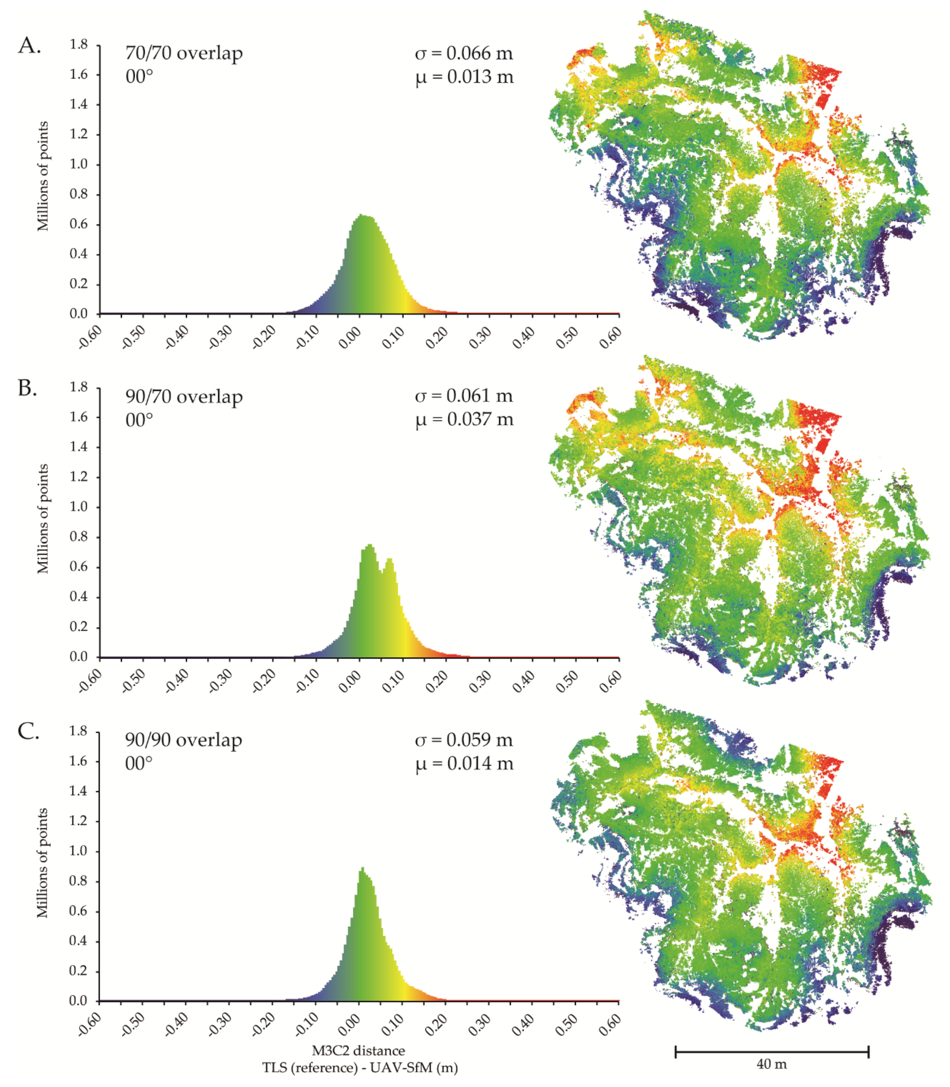
Figure 5.
M3C2-calculated distance between TLS reference dataset and UAV–SfM data sets collected with nadir camera angles and cross-hatch flight lines (NSEW) with various image overlap settings: (A) 70/70, (B) 90/70, and (C) 90/90. Positive values indicate UAV–SfM surface above TLS reference surface; negative values suggest UAV–SfM surface below. Note the systematic distribution of error with low points (near the center of the field area) higher than the reference dataset and high points (near the perimeter of the field area) lower than the reference dataset. This systematic error is similar to that noted by James and Robson [21] and is present regardless of overlap.

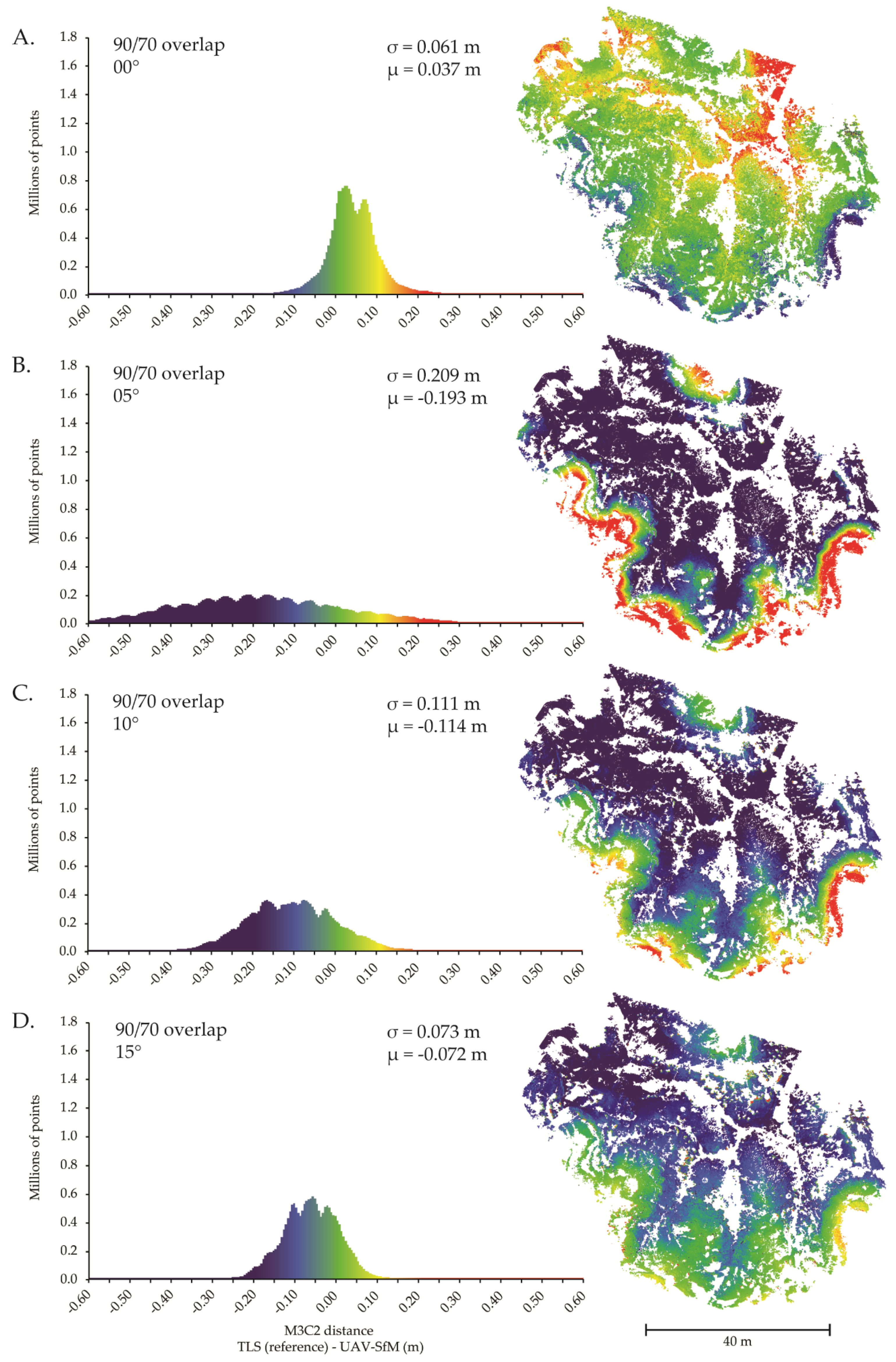
Figure 6.
M3C2-calculated distance between TLS reference dataset and UAV–SfM image sets collected with 90/70 overlap, cross-hatch flight lines (NSEW), and a single camera angle; (A) 00° (nadir); (B) 05°; (C) 10°; (D) 15°; (E) 20°; (F) 25°; (G) 30°; (H) 35°. Positive values indicate UAV–SfM surface above TLS reference surface; negative values suggest UAV–SfM surface below.


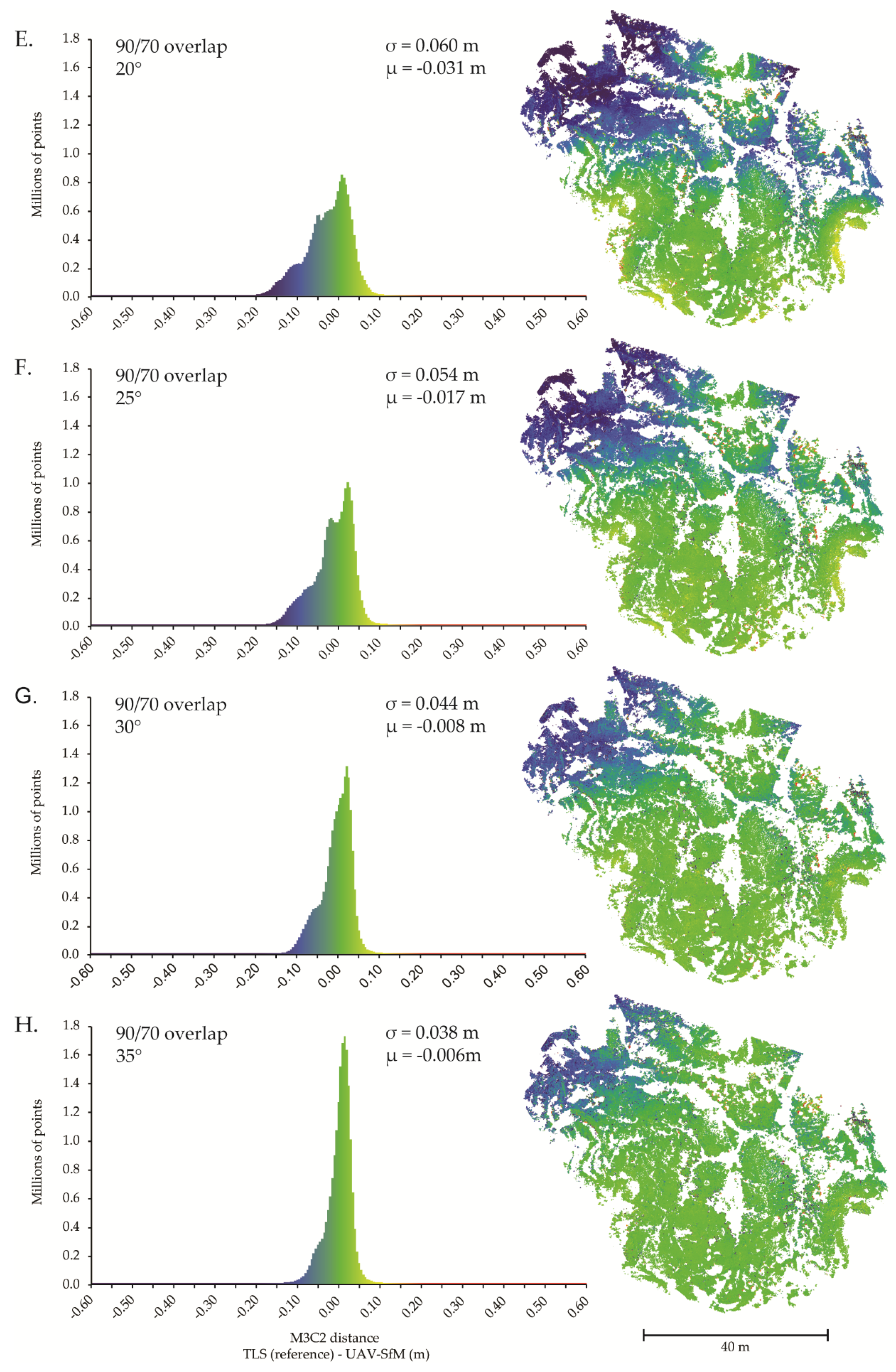
Figure 7.
M3C2-calculated distance between TLS reference dataset and UAV–SfM combination image sets: (A) 70/70—05° BoxIO; (B) 70/70—20° BoxIO; (C) 70/70—35° BoxIO; (D) 90/70—05° BoxIO; (E) 90/70—20° BoxIO; (F) 90/70—35° BoxIO. See Figure 2 for description of flight patterns. Positive values indicate UAV–SfM surface above TLS reference surface; negative values suggest UAV–SfM surface below.


Figure 8.
M3C2-calculated difference between TLS reference dataset and various UAV–SfM combination datasets with different image configurations: (A) standard deviation, 70/70 overlap combinations; (B) standard deviation, 90/70 overlap combinations; (C) mean difference, 70/70 overlap combinations; (D) mean difference, 90/70 overlap combinations. See Figure 2 for description of flight patterns.


Table 1.
Recommended oblique image angles for supplementing structure-from-motion (SfM) nadir image blocks from the literature.
Table 1.
Recommended oblique image angles for supplementing structure-from-motion (SfM) nadir image blocks from the literature.
| Imaging Strategy | Author | Suggested Angle | Additional Notes |
|---|---|---|---|
| Airborne UAV 1 | Bemis et al. [6] | 10–20° | |
| James and Robson [21] | 20–30° | ||
| Markelin et al. [61] | 25–30° | ||
| Harwin et al. [52] | 45–65° | ||
| Carbonneau and Dietrich [54] | 20–45° | >10% of image sets | |
| Carvajal-Ramirez et al. [15] | 35° | Orthogonal to surface | |
| James et al. [62] | 20° | ||
| Rossi et al. [25] | 60° | Orthogonal to surface | |
| Agüera-Vega et al. [18] | 45° | ||
| Ground-based | Moreels and Perona [63] | <25–30° | |
| Gienko and Terry [64] | <20° | Angle of incidence >40° | |
| James and Robson [21] Stumpf et al. [65] | 10–20° <30° | ||
| Multicam | Fritsch and Rothermel [66] | 45° | Higher angles of intersection are optimal |
| Rupnik et al. [67] | 35 or 45° | Higher tilt angle was more robust but more susceptible to occlusions |
1 Uninhabited/unmanned Aerial Vehicle.
Table 2.
UAV–SfM processing scenarios.
| Overlap | Image Pattern 1 | Camera Angles | |
|---|---|---|---|
| Single camera angle | 90/90 or 90/70 or 70/70 | Image block (parallel flight lines) | 0–35° |
| Combination datasets | 90/70 or 70/70 | BoxO BoxI BoxIO Single arcs Double arcs | Image block at nadir + image pattern collected with an oblique camera angle (5–35°) |
1 See Figure 2 for description of combination patterns.
Table 3.
Processing settings in Pix4Dmapper selected for all UAV–SfM scenarios.
| Step | Processing Option | Setting |
|---|---|---|
| 1. Initial processing | Keypoint image scale Matching image pairs Calibration | Full Aerial grid or corridor Standard (AAT 1, BBA 2, camera self-calibration) |
| 2. Point cloud densification | Image scale Point density Minimum number of matches Matching window size | 1 (original image size, slow) Multiscale Optimal 4 9 × 9 pixels |
1 Automatic aerial triangulation (AAT); 2 Bundle block adjustment.
© 2019 by the authors. Licensee MDPI, Basel, Switzerland. This article is an open access article distributed under the terms and conditions of the Creative Commons Attribution (CC BY) license (http://creativecommons.org/licenses/by/4.0/).
Share and Cite
MDPI and ACS Style
Nesbit, P.R.; Hugenholtz, C.H. Enhancing UAV–SfM 3D Model Accuracy in High-Relief Landscapes by Incorporating Oblique Images. Remote Sens. 2019, 11, 239. https://0-doi-org.brum.beds.ac.uk/10.3390/rs11030239
AMA Style
Nesbit PR, Hugenholtz CH. Enhancing UAV–SfM 3D Model Accuracy in High-Relief Landscapes by Incorporating Oblique Images. Remote Sensing. 2019; 11(3):239. https://0-doi-org.brum.beds.ac.uk/10.3390/rs11030239
Chicago/Turabian StyleNesbit, Paul Ryan, and Christopher H. Hugenholtz. 2019. "Enhancing UAV–SfM 3D Model Accuracy in High-Relief Landscapes by Incorporating Oblique Images" Remote Sensing 11, no. 3: 239. https://0-doi-org.brum.beds.ac.uk/10.3390/rs11030239
Note that from the first issue of 2016, this journal uses article numbers instead of page numbers. See further details here.