Modeling Polycentric Urbanization Using Multisource Big Geospatial Data

Abstract

Understanding the dynamics of polycentric urbanization is important for urban studies and management. This paper proposes an analytical model that uses multisource big geospatial data to characterize such dynamics to facilitate policy making. There are four main steps: (1) main centers and subcenters are identified using spatial cluster analysis and geographically weighted regression (GWR) based on Visible Infrared Imaging Radiometer Suite (VIIRS)/NPP and social media check-in data; (2) the built-up areas are extracted by using Defense Meteorological Satellite Program—Operational Linescan System (DMSP/OLS) gradient images; (3) the economic corridors that connect the main center and subcenters are constructed using road network data from Open Street Map (OSM) with the least-cost distance method; and (4) the major urban development direction is identified by analyzing the changes in built-up areas within the economic corridors. The model is applied to three major cities in northeastern, central, and northwestern China (Shenyang, Wuhan, and Xi’an) from 1992 to 2012.

1. Introduction

Urbanization is a complex phenomenon that is accompanied by profound land-cover/land-use changes and social dynamics [1,2]. Urbanization leads to the redistribution of social and economic resources, thereby possibly transforming the landscape from a monocentric to a polycentric structure. Typically, a main urban center has the highest population density in its region, and features a central business district [3]. Subcenters, which have higher population densities than adjacent regions, are typically distributed around the main center [4]. Polycentric urbanization is a process of interaction between a main center and subcenters by which the built-up areas of the main center and subcenters expand, thereby gradually approaching one another [5].

Economic corridors within polycentric cities typically feature high-density road networks that connect main centers and subcenters [6]. Polycentric urbanization in the developed countries and regions is mainly manifested in the generation of polycentric employment subcenters, while the developing world typically witnesses the expansion of built-up areas [7]. China has both features [8]. By studying polycentric urbanization, the evolution of the relationship between main centers and subcenters can be analyzed for enhanced urban management [9].

In recent years, polycentric urban structure and polycentric urbanization have been studied extensively. Most studies rely on aggregate-level socioeconomic data and adopt the methods such as the data thresholding method, nonparametric analysis, and principal component analysis [4,7,10,11,12]. The central business districts (CBDs) of Chinese cities are considered the main centers in polycentric cities [13,14,15]. These methods assume that the main centers or subcenters are of a higher population or employment density than the surrounding areas. These centers are identified by analyzing the density and the degree of polycentric urbanization, which can be estimated from the density change. However, the coarse spatial and temporal scales of socioeconomic data and the arbitrary definition of the thresholds limit the use of these methods. For example, polycentric structure detection sometimes relies on subjectively set density thresholds [7], and nonparametric analysis might require the manual selection of the main centers [4].

Remote sensing provides raster data support. Due to the time issue of MODIS data and the classification difficulty of Landsat data, nighttime light remote sensing data have been widely used in urban and regional analysis [16,17]. For example, built-up areas that are extracted from nighttime light data can cover the parks within cities that are ignored by Landsat data [18]. In the Defense Meteorological Satellite Program—Operational Linescan System (DMSP/OLS) and Visible Infrared Imaging Radiometer Suite (VIIRS)—NPOESS Preparatory Project, the urban structure has been studied, e.g., via the Gaussian volume model with DMSP/OLS data [19] and the topographical metaphor method with VIIRS/NPP data [20]. These methods examine the objective evidence of interaction between spectral changes of nighttime light data and urban structural dynamics. However, nighttime light data contain lights from roads, ports, and industrial areas, which reduces the accuracy of urban structure detection [21]. Nighttime light data are more often used to analyze the spatial coverage change of built-up areas instead of the spatial expansion direction [13,22,23]. Recently, social media data have provided new opportunities for analyzing the population distribution and human activity at the final scale [14,15]. A polycentric urban structure can be analyzed via spatial cluster analysis and geographically weighted regression (GWR) by integrating Weibo check-in data and VIIRS/NPP data [3].

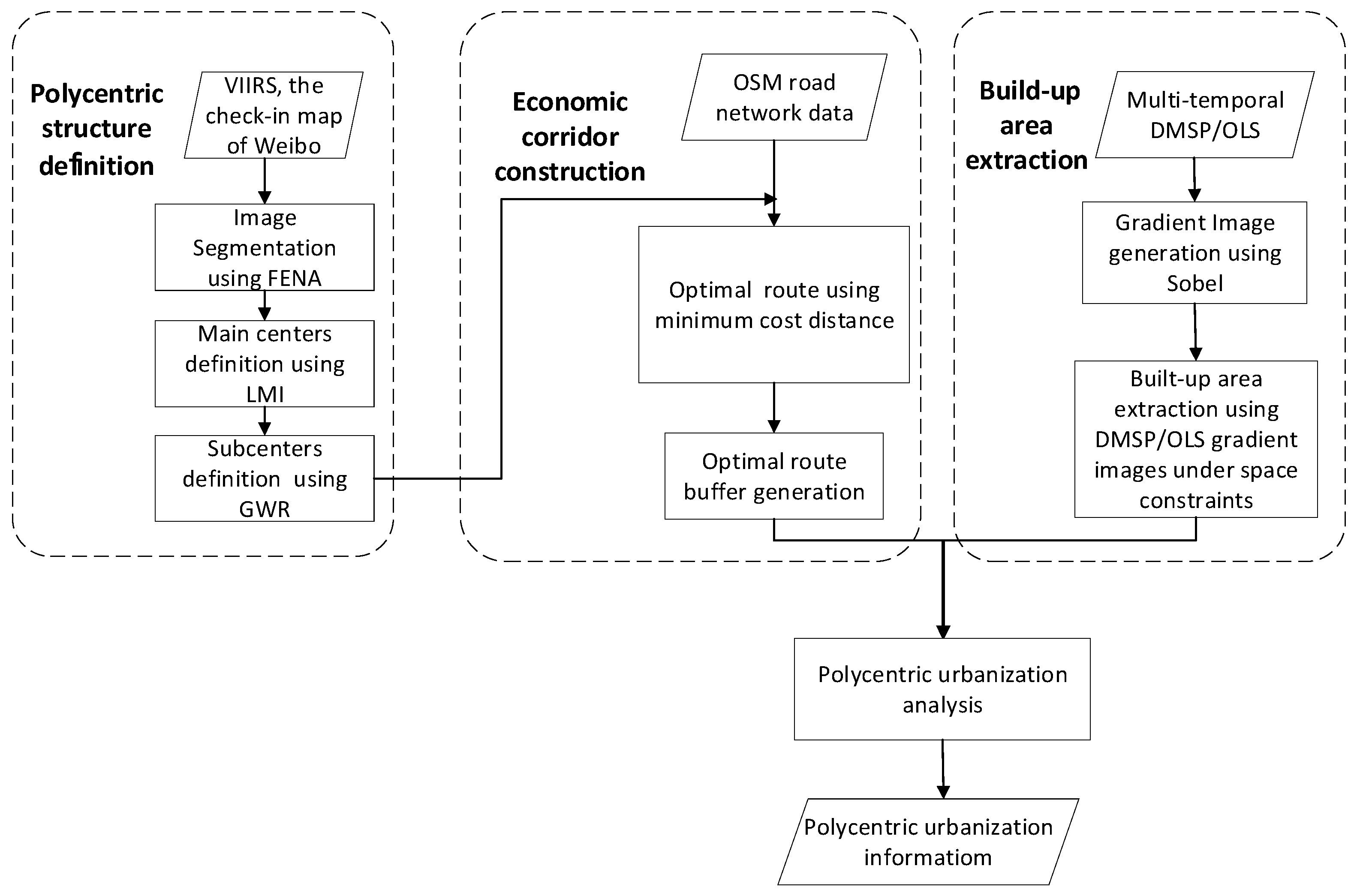
In this paper, we develop a polycentric urbanization analytical model for identifying the main urban expansion direction. This model can enhance the understanding of polycentric urbanization at fine spatial and temporal scales. First, we perform relative radiation correction for multitemporal DMSP/OLS data in the data preprocessing step. Second, Local Moran’s I (LMI) and geographically weighted regression (GWR) are used to define main centers and subcenters. Third, the minimum cost distance and the optimal route buffer are used to construct economic corridors. Meanwhile, by using DMSP/OLS gradient images under spatial constraints, multitemporal built-up areas are extracted. Finally, the changes in the multitemporal built-up areas are analyzed within the economic corridors. Three major Chinese cities are examined. In addition, our approach is compared with other methods. Finally, we summarize the main advantages and disadvantages of the proposed method.

2. Materials and Methods

2.1. Study Areas

We select three major cities in China as the study areas: Shenyang, Wuhan and Xi’an. These cities serve as the centers of politics, economy, culture, education, and transportation of their regions. Shenyang is the largest city in northeastern China, with a total area of 3423 square kilometers and a permanent population of 8.2 million in 2016. Wuhan is the most populous city in central China. The total area of the municipal administrative jurisdiction is 1372 square kilometers, and the permanent population was 10.7 million in 2016. It is divided by the Hanjiang River and Yangtze River into the Hanyang, Hankou, and Wuchang districts. Xi’an is the largest city in northwestern China, with a total area of 815 square kilometers and a permanent population of 8.7 million in 2016.

2.2. Data

2.2.1. Nighttime Light Imagery

DMSP/OLS data and VIIRS/NPP data are currently the most widely used nighttime light remote sensing data. DMSP/OLS data range from 1992 to 2013 with a spatial resolution of 1000 m. For this research, stable DMSP/OLS data for 1992, 1996, 2000, 2004, 2008, and 2012 are selected, and the interference from sunlight, moonlight, clouds, wildfires, lightning, and auroras is removed. VIIRS/NPP data cover 2012 to the present, with a spatial resolution of 500 m. To ensure that the time was consistent with the Weibo check-in data, we selected VIIRS/NPP data from October 2014. Stable VIIRS/NPP data were used to generate new image processing units, which reduced the spatial instability of the Weibo check-in data [3].

2.2.2. Social Media Data

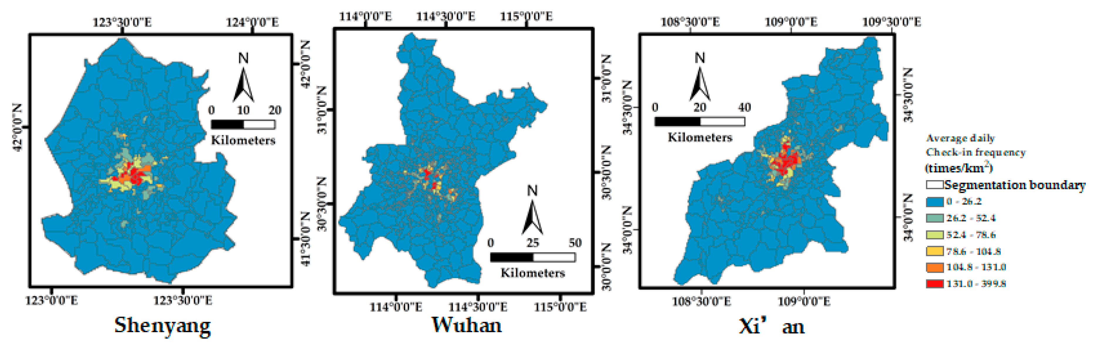
Social media data can describe the time and location of human activities [24]. Weibo is one of the most popular and widely used social media and networking platforms in China. The number of active Weibo users reached 222 million in September 2015, 85% of whom were mobile active users [25]. Due to restricted data permission, we only have the Weibo check-in data from October 2014 for identifying main centers and subcenters.

2.2.3. Road Network Data

Urbanization is accompanied by the extension and expansion of road networks [26]. Open Street Map (OSM) is an open-source editable map service platform of road network data that was jointly created by the public [27]. Road network data from OSM have been applied in urban analysis [28,29]. In this paper, such data were used to construct economic corridors that connect main centers and subcenters.

3. Methodology

3.1. Data Preprocessing

The proposed model is illustrated in Figure 1. To improve the stability and continuity of the multitemporal DMSP/OLS data, a relative radiation correction algorithm that uses the binary regression model is applied [30]. This method assumes that the gray values of the DMSP/OLS data in the reference area do not change. The relationship between each corrected gray value and the corresponding original gray value is established by a quadratic regression equation. The DMSP /OLS data for 1992, 1996, 2000, 2004, 2008, and 2012 are corrected.

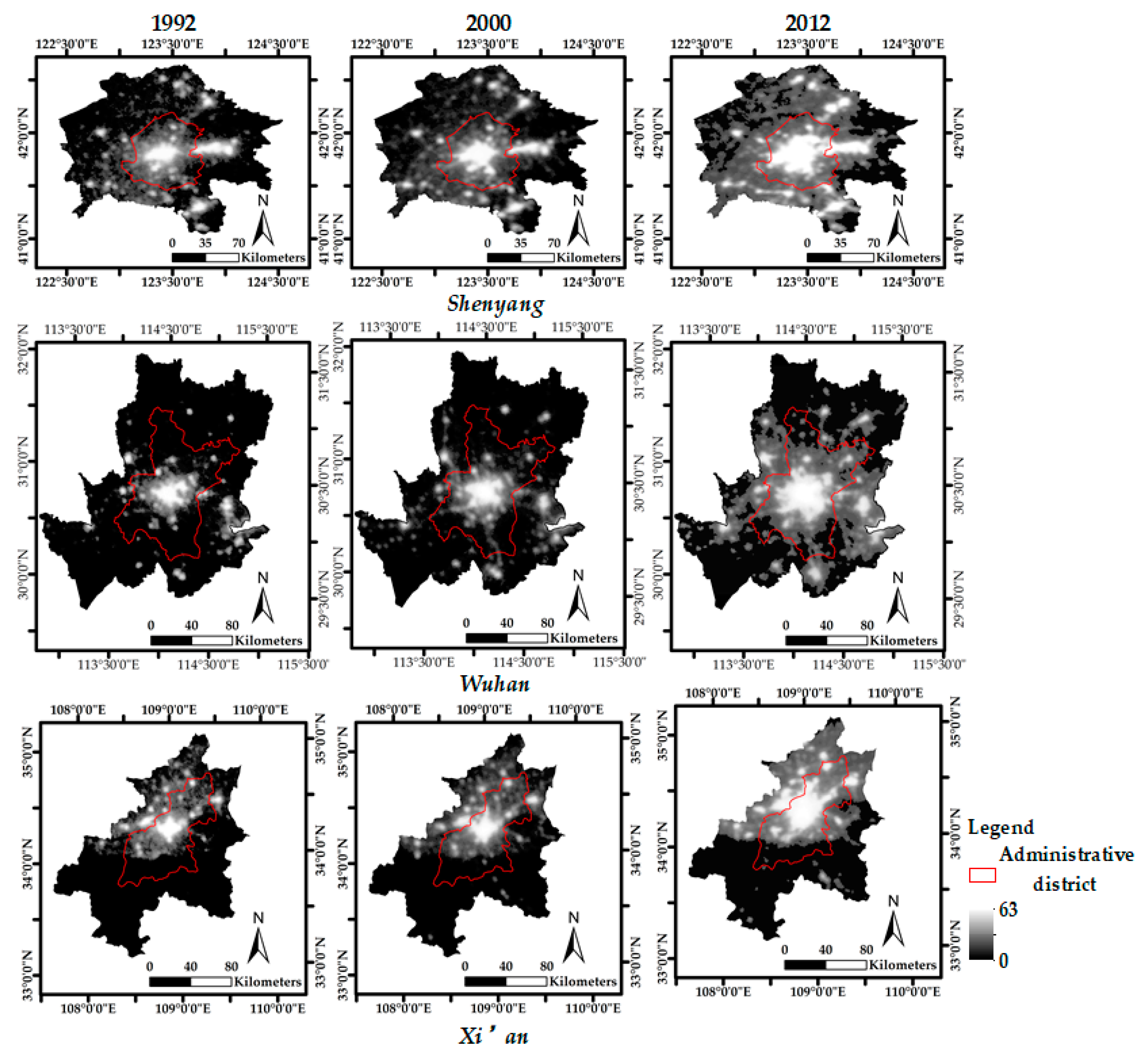
The corrected DMSP/OLS data is set to Asia Lambert conformal conic projection with a resampling resolution of 500 m. The VIIRS/NPP data and Weibo check-in data are set to the same projection and sampling resolution. The relative radiation-corrected DMSP/OLS data for 1992, 2000, and 2012 are shown in Figure 2.

3.2. Polycentric Urban Structure Definition

3.2.1. Observation Units

Social media data can be used to identify population centers [24,31]. Due to the instability of social media data [31], we use the method that was proposed by [3] to integrate social media data with VIIRS/NPP data. The image processing method, which is based on objects, uses a cluster of pixels that have the same homogeneity as a processing unit. The fractal net evolution approach (FNEA) segmentation algorithm is widely employed in remote sensing image segmentation [32]. In this paper, FNEA is used to perform image segmentation on VIIRS/NPP data and Weibo check-in data to construct new processing units. The Weibo check-in data and VIIRS/NPP data are assigned equal weight, which can effectively reduce the influence of nighttime light data. Three parameters (scale, shape, and compactness) affect the segmentation results. The shape parameter is set to 0.1 to increase the influence of the spectrum. The compactness parameter is set to 0.5 to balance the convergences of image objects with the ratio of the perimeter to the area. Since the scale parameter is application-dependent, we set it to five. To ensure integrity, the image objects that have an area of less than one square kilometer are merged.

3.2.2. Main Center

The main center is the core of the city, and has a high level of population activity. The main center is the center of gravity of the main center region. In this paper, the main center region and main center are defined based on the local Moran index [3]. The mean of the Local Moran’s I values of the Weibo check-in data of each image object is used to merge the image objects that have high positive z-score values (larger than 1.96) into sets of image objects. The image object sets that have the largest area are selected as the main center region. The center of gravity of the main center region is considered the main center.

3.2.3. Subcenter

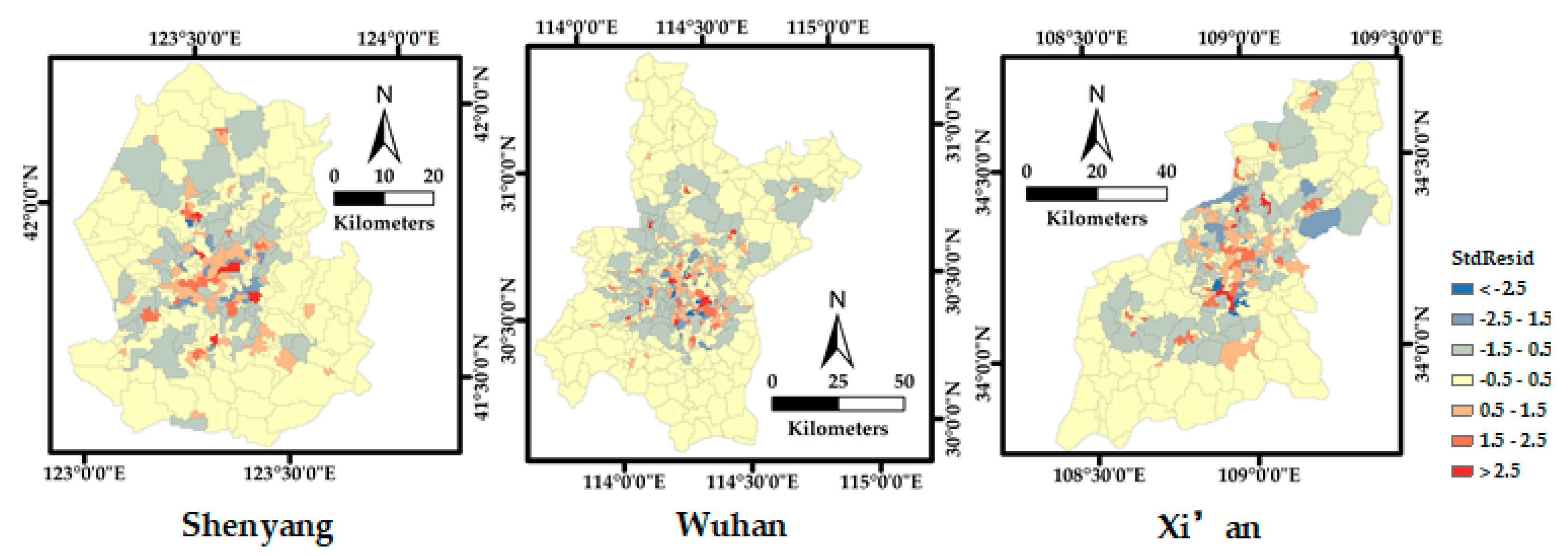
The subcenter regions represent the aggregation of high-level economic activities outside the main center region. The human activity density in the subcenter region substantially exceeded that of its adjacent region, which is reflected in the image as an island of brightness. We define the subcenter region using geographically weighted regression (GWR) and Jenks’ natural breaks classification (NBC). GWR provides local regression analysis for observational data. GWR combines dependent variables and explanatory variables for elements that fall within the bandwidth of each target element:

$${\mathrm{y}}_i={\beta }_0(u_i,v_i)+{\displaystyle \sum _k{\beta }_k}(u_i,v_i)d_{ik}+{\epsilon }_i$$

(1)

where ${\mathrm{y}}_i$ is the square root of the Weibo check-in mean density of image object $i$, ${\beta }_0(u_i,v_i)$ is the intercept, ${\beta }_k(u_i,v_i)$ is the local estimation coefficient for the $k$th independent variable of image object $i$, and ${\epsilon }_i$ is the residual [33]. A Gaussian kernel was used to establish the local distance function, and the optimal bandwidth was identified via cross-validation. Since the subcenter had a higher density of Weibo check-in data than the surrounding area, image objects that had a standard deviation that exceeded 1.96 were selected as the candidate subcenters [3]. The subcenter regions were acquired after the candidates that had lower human density or area over the entire study area had been filtered using NBC. The centers of gravity of the subcenter regions were extracted to represent the subcenters.

3.3. Built-Up Area Extraction

DMSP/OLS data are highly correlated with economic activity, population density, and impermeable areas [23,34]. The fluctuations of the DMSP/OLS gray values correspond to the dynamics of the economy and the density of the built-up area. The brightness values of DMSP/OLS data change with the spatial economic fluctuations, thereby providing a basis for built-up area extraction. Suburban areas are transitional belts between built-up areas and rural areas, where the changes of DMSP/OLS brightness are obvious. This paper proposes an automatic built-up area extraction method that uses DMSP/OLS gradient images under spatial constraints. A two-step strategy is used to implement this method:

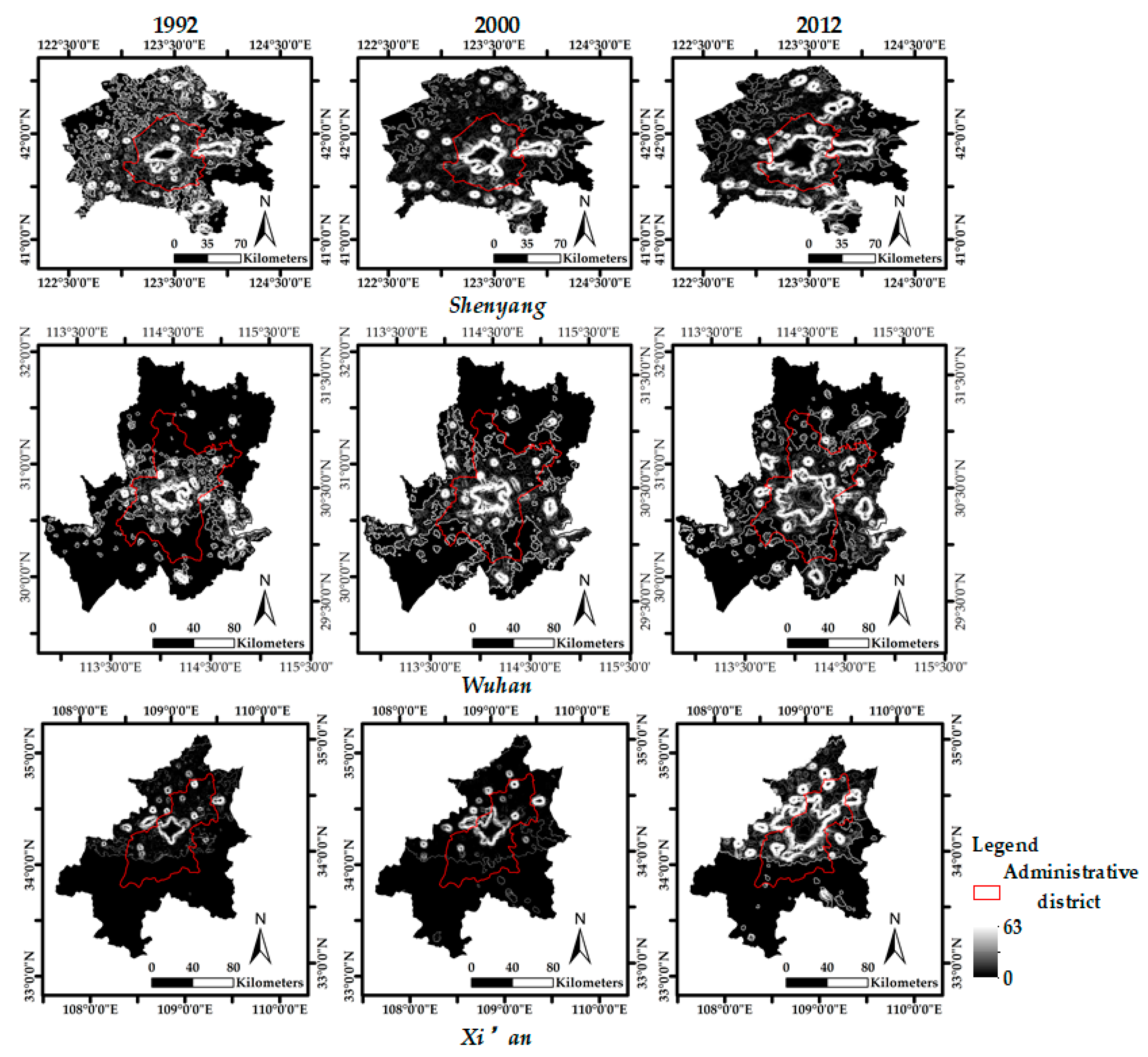
(1) DMSP/OLS gradient image construction. Sobel operators are used to obtain gradient images [35]. The size of each operator is $3\times 3$. Gradient images of multitemporal DMSP/OLS data are shown in Figure 3. To highlight the features of the images, a percent truncated stretch has been applied to each of the images.

As shown in Figure 3, the built-up areas exhibit slight changes in the corresponding gray values, and their gradient images show low-gray-value areas with strong homogeneity. In contrast, the suburban areas correspond to high degrees of gray value change. The suburban gradient images show high-gray-value areas with weak homogeneity, and the main spatial features are large closed ring areas that surround the built-up area. Finally, the rural areas correspond to small degrees of gray value change. The rural gradient images show low gray value regions with strong homogeneity, which are located in the outer areas of the suburban areas. After Sobel processing, the DMSP/OLS data are divided into high gray value regions with weak homogeneity and low gray value regions with strong homogeneity.

(2) Built-up area extraction under spatial constraints. Multi-scale segmentation that is based on FENA is performed on the gradient images of DMSP/OLS. To ensure that the image objects have strong homogeneity, the segmentation scale is set to two. The shape parameter is set to 0.1, and the compactness parameter is set to 0.5. To extract suburban areas, the suburban gray value range is set to:

$$D{N}_{\min }\le D{N}_{\mathrm{suburb}}\le D{N}_{\max }$$

(2)

where $D{N}_{\mathrm{suburb}}$ is the gray value that corresponds to the suburban areas, $D{N}_{\min }$ is the suburban lower-limit gray value, and $D{N}_{\max }$ is the suburban upper-limit value. $D{N}_{\min }$ is obtained via the gray value increment operator:

$$D{N}_{\min }=1+D{N}_{\mathrm{interval}}\ast n$$

(3)

where the incremental gray value step, which is denoted as $D{N}_{\mathrm{interval}}$, is set to 0.5, and n is the number of increases. Since the suburban areas are closed, $D{N}_{\min }$ is the gray value at the last time when the suburban ring closed. To obtain a full suburban ring, the spatial extent of the DMSP/OLS data is extended to the adjacent regions. The multitemporal suburban gray limits are listed in

Table 1. Multitemporal suburban gray limits.

Region	1992	2000	2012
Shenyang	5	7	5
Wuhan	4.5	6	4
Xi’an	4	6	4.5

. According to Table 1, the lower-limit gray value is distributed in the range of 4.5 to 7, and is stable.

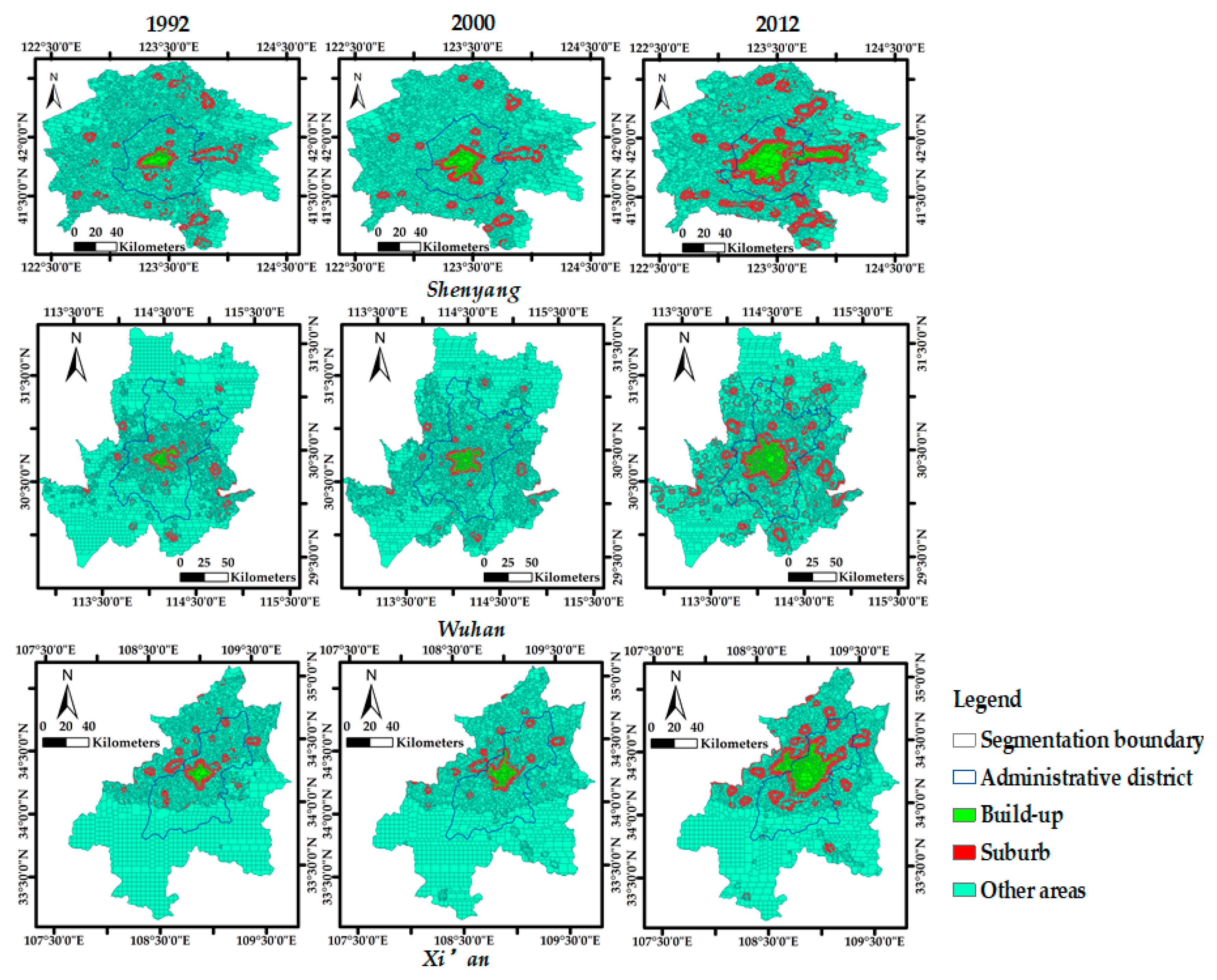
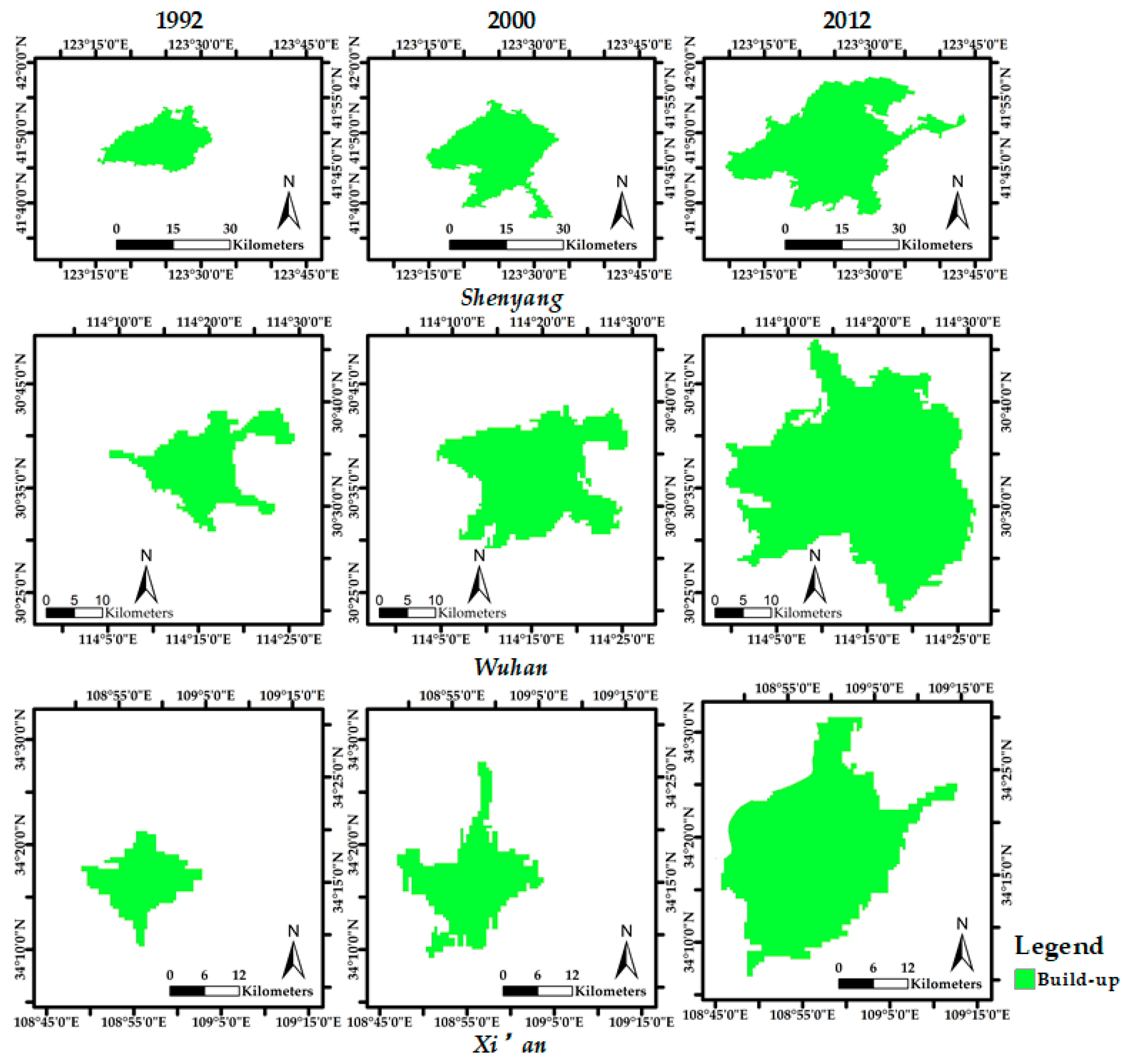
The suburban classification results of Shenyang, Wuhan, and Xi’an are shown in Figure 4. The green regions outside the suburbs correspond to the countryside. According to Figure 5, the coverage of the built-up areas continues to expand, and small towns around the main built-up areas are gradually being integrated.

3.4. Economic Corridor

An economic corridor is a narrow delineated area that connects major economic nodes, along with transportation infrastructure such as roads, railways, and canals [6]. As the main traffic infrastructure, the density of the road network can reflect the economic status of a city [36]. The collaborative development of a main center and a subcenter is accompanied by the flow of resources. The main center provides financial and commercial resources for subcenters, while subcenters provides residential, industrial facilities, and food for the main center. This paper proposes an economic corridor construction method that uses the minimum cost distance. The first step is optimal route extraction. The minimum cost distance algorithm uses raster data that describe the cost of calculating the minimum cost distance between the focus cells to the other neighboring cells. The road network density cost data are obtained via inverse processing of the road network data. The road network density cost data are expressed as:

$$D_p=R_{\max }-R_p$$

(4)

where $D_p$ is the gray value of the road network density cost data at point $p$, $R_{\max }$ is the maximum gray value of the road network density raster data, and $R_p$ is the gray value of the road network density data at point $p$. The second step is to generate the buffer for the optimal route and construct the economic corridor. The buffer extends two kilometers from both sides of the optimal route.

3.5. Polycentric Urbanization Analysis

The multitemporal built-up areas are denoted as ${\mathrm{B}}_1,\dots ,{\mathrm{B}}_m,\dots ,{\mathrm{B}}_M$, where ${\mathrm{B}}_m$ is a polygon vector that records the properties of built-up areas in year m. The area of the built-up area in year m is recorded as ${\mathrm{A}}^m$. The built-up area growth rate (BAGR), which is denoted as ${\mathrm{R}}^m$, from year m-1 to year m is expressed as:

$${\mathrm{R}}^m=\frac{{\mathrm{A}}^m-{\mathrm{A}}^{m-1}}{{\mathrm{A}}^{m-1}}$$

(5)

The number of economic corridors is the same as the number of subcenters. The economic corridors are denoted as $C_1,\dots ,C_n,\dots ,C_N$, where $C_n$ is a polygon of the economic corridor. The built-up area of economic corridor n in year m is denoted as ${\mathrm{A}}_n^m$. The BAGR of the economic corridor, which is denoted as ${\mathrm{r}}_n^m$, is expressed as:

$${\mathrm{r}}_n^m=\frac{{\mathrm{A}}_n^m-{\mathrm{A}}_n^{m-1}}{{\mathrm{A}}_n^{m-1}}$$

(6)

A large value of ${\mathrm{r}}_{\mathrm{n}}^{\mathrm{m}}$ corresponds to the rapid development of economic corridor n from year m-1 to year m. It is inferred that subcenter n was the major spatial expansion direction during that period of time.

4. Results

4.1. Polycentric Structure

4.1.1. Segmentation

Using FENA to segment the Weibo check-in data and the VIIRS/NPP data, Shenyang, Wuhan, and Xi’an are divided into 268, 487, and 337 image objects, respectively. The segmentation results are shown in Figure 5.

The smaller image objects are mainly distributed in the built-up areas. The larger image objects are mainly distributed in the outer regions of administrative divisions, most of which are located in rural areas. Since the Weibo check-in density data and the VIIRS/VPP data reflect the human activity density, the gray values are larger in the areas where the human activity density is higher. This is why the image objects that are within the built-up areas are smaller, and the image objects that are within the rural areas are larger.

4.1.2. Polycentric Structure

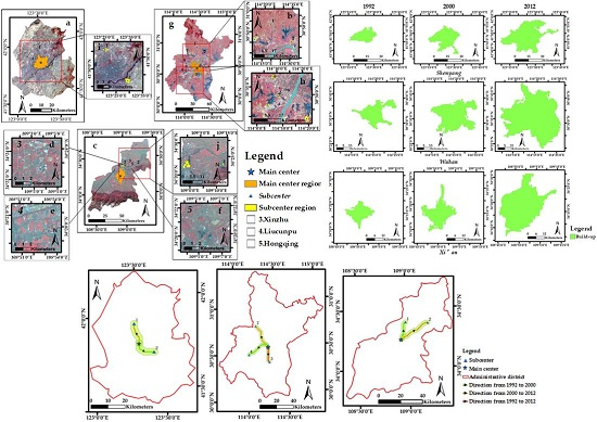
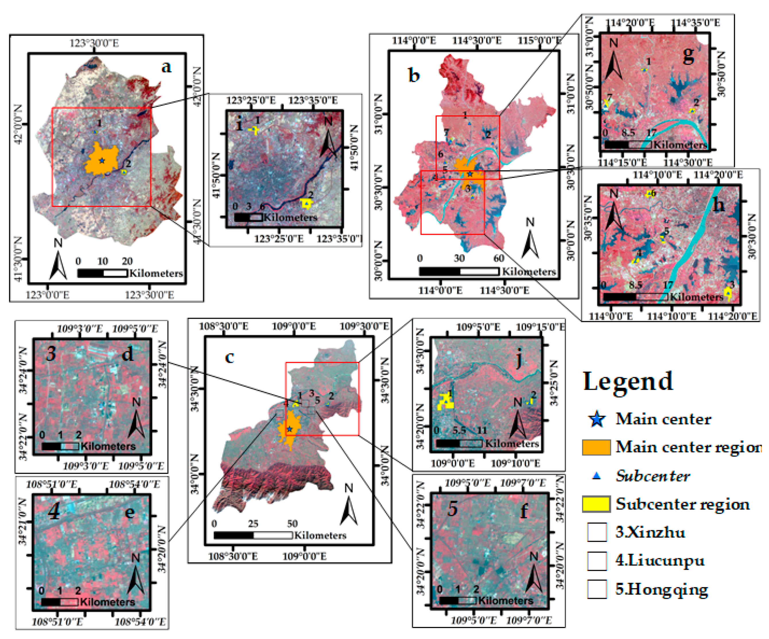
The main center regions, main centers, subcenter regions, and subcenters are shown in Figure 6. The main center region of Shenyang is 130.75 square kilometers, which accounts for 4.1% of the total area. There are two subcenters to the north and south of the main center region. The area of the main center region of Wuhan is 311.75 square kilometers, which accounts for 3.72% of the total area. There are seven subcenters to the north, west, and south of the main center region. The area of the main center region of Xi’an is 195 square kilometers, which accounts for 3.86%. There are two subcenters to the north and northeast of the main center area.

The results of the GWR model are presented in Figure 7 and

Table 2. Results of the GWR model.

Parameters	Shenyang	Wuhan	Xi’an
Residual Squares	646.22	1997.91	1246.41
Sigma	1.98	2.33	2.23
AICc	1209.27	2289.09	1557.75
R2	0.85	0.78	0.81

. A satisfactory fitting degree is realized for each of the three cities, with R² exceeding 0.75.

The results for the subcenters are listed in

Table 3. Results for subcenters.

GWR Estimation and Subcenters	Shenyang	Wuhan	Xi’an
Number of image objects that have higher standard residuals	9	18	16
Number of image objects that overlap and are adjacent to main center regions	3	9	8
Number of image objects that belong to the final level of NBC* (either density or area)	4	2	6
Number of image objects that belong to subcenter regions	2	7	2
Final number of image objects that belong to subcenter regions	2	7	2

NBC*: natural breaks classification.

. For Shenyang, Wuhan, and Xi’an, the numbers of image objects for which the GWR residuals exceed 1.96 are 9, 18, and 16, respectively. The numbers of image objects that overlap and are adjacent to the main center regions are three, nine, and eight, respectively. The numbers of image objects that belong to the final level of NBC of the Weibo check-in density or area are four, two, and six, respectively. The numbers of image objects that belong to subcenter regions are two, seven, and two, respectively. Since there is no adjacency relationship among these image objects, the numbers of image objects that belong to subcenters are two, seven, and two, respectively.

4.2. Built-Up Areas

The extraction results of the built-up areas are shown in Figure 8. The statistics of the built-up areas are listed in

Table 4. Statistics of the built-up areas (km²).

Region	1992	2000	2012	1992–2000	2000–2012	Mean	Max
Shenyang	202	351	706	73.76%	101.14%	87.45%	2000–2012
Wuhan	271	492	1166	81.55%	136.99%	109.27%	2000–2012
Xi’an	174	300	821	72.41%	173.67%	123.04%	2000–2012

. According to Figure 8 and Table 4, the built-up areas from the time series exhibited steady growth.

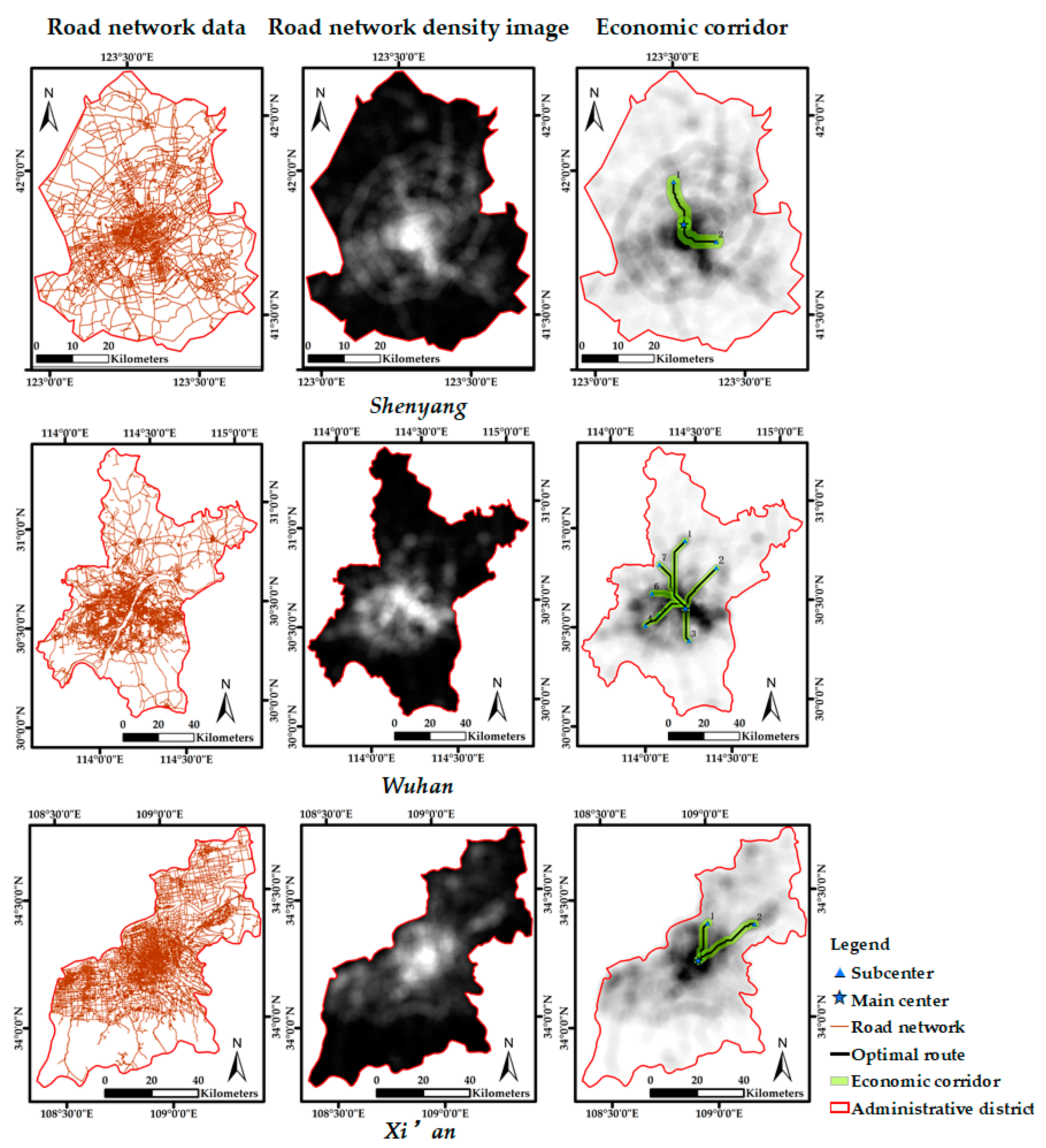
4.3. Economic Corridors

The economic corridors are shown in the third column of Figure 9. The urban core has the highest road network density. The background image shows the road network density cost data. The higher gray value regions have a higher cost density, and the lower gray value areas have a lower cost density. The black lines represent the optimal routes that connect the main centers and the subcenters, which were extracted via the minimum cost distance algorithm. The optimal routes pass through the regions with the lowest costs, which correctly reflects the optimal routes of transport between the main centers and the subcenters.

4.4. Polycentric Urbanization

The changes in the urban built-up areas are summarized in Table 4. The built-up areas of Shenyang, Wuhan, and Xi’an exhibited fast growth rates from 2000 to 2012 of 101.14%, 136.99%, and 173.67%, respectively. The mean values of the GRBAs for the three cities are 87.45%, 109.27%, and 123.04%, respectively. From 1992 to 2000, the urbanization of Xi’an was the fastest, followed by Wuhan and Shenyang.

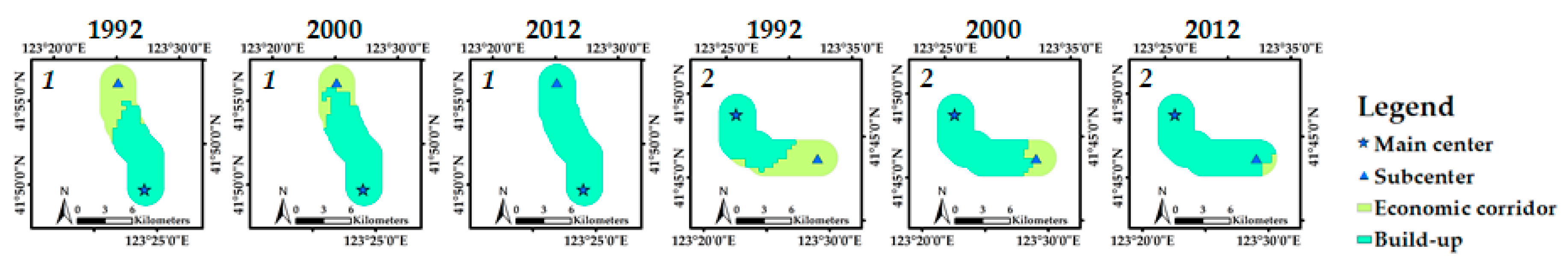
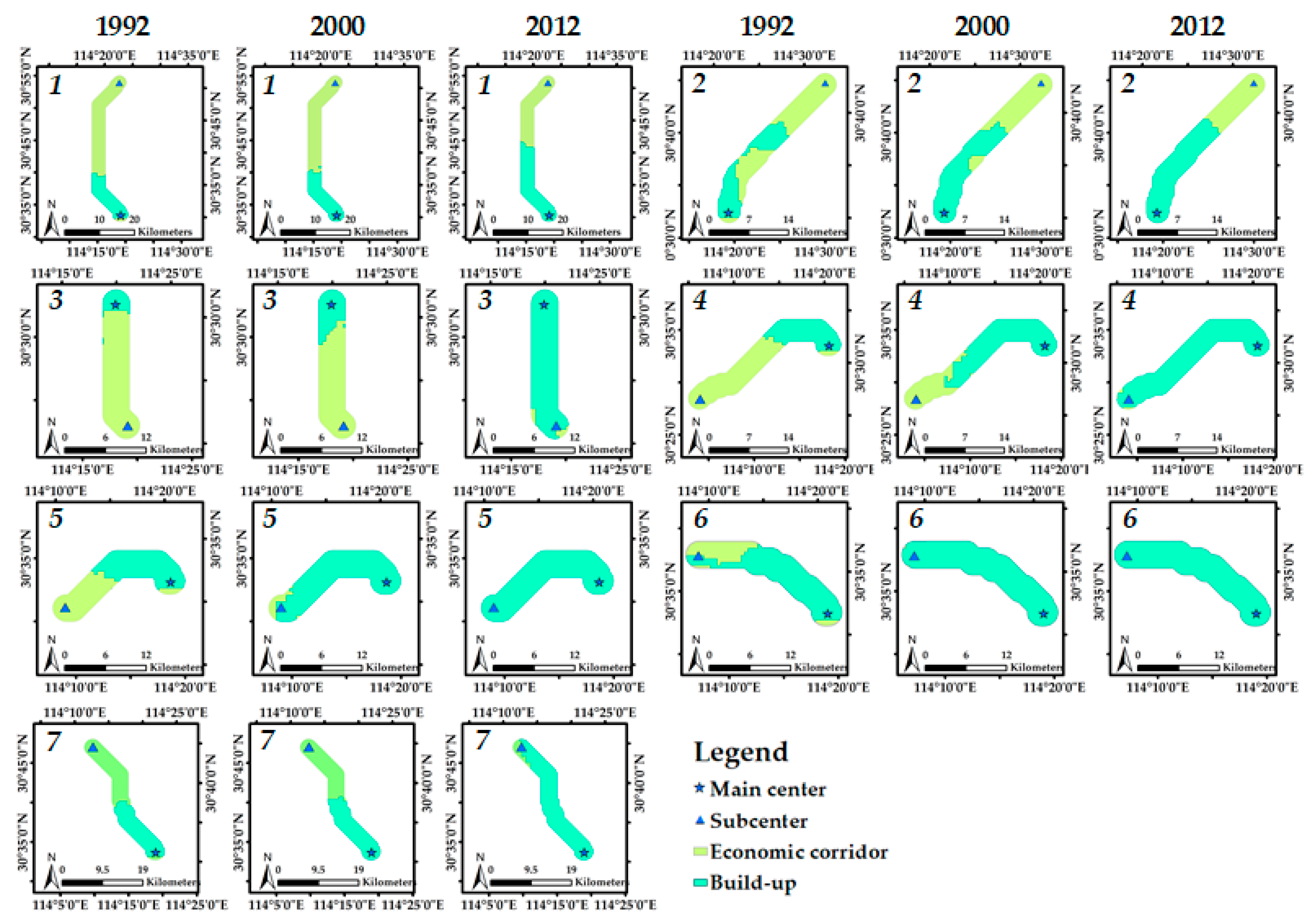
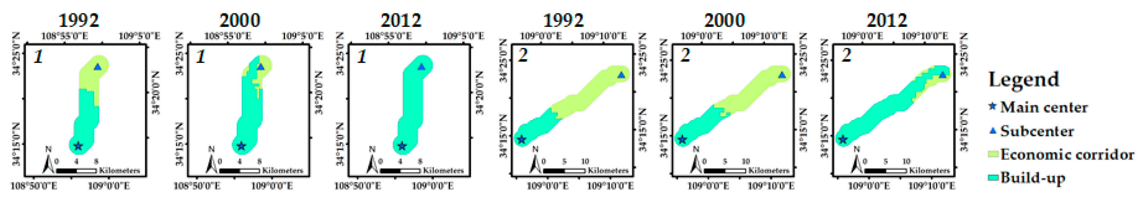
The built-up areas of the economic corridors for Shenyang, Wuhan, and Xi’an are shown in Figure 10, Figure 11 and Figure 12, respectively. The multitemporal built-up area statistics of the economic corridors for Shenyang, Wuhan, and Xi’an are listed in

Table 5. Statistics of the built-up areas within the economic corridor for Shenyang.

Number	1992		2000		2012		All Area	1992–2000	2000–2012	Mean	Max
	A	R	A	R	A	R
1	41	0.65	48	0.76	63	1	63	17.07%	31.25%	24.16%	2000–2012
2	38	0.59	53	0.83	61	0.95	64	39.47%	15.09%	27.28%	1992–2000

A: Area; R: Ratio.

,

Table 6. Statistics of the built-up areas within the economic corridor for Wuhan.

Number	1992		2000		2012		All Area	1992–2000	2000–2012	Mean	Max
	A	R	A	R	A	R
1	60	0.32	67	0.36	97	0.52	185	11.67%	44.78%	28.23%	2000–2012
2	50	0.38	74	0.57	83	0.64	130	48.00%	12.16%	30.08%	1992–2000
3	11	0.13	23	0.26	84	0.97	87	109.09%	265.22%	187.16%	2000–2012
4	51	0.39	91	0.7	128	0.98	130	78.43%	40.66%	59.55%	1992–2000
5	51	0.56	85	0.93	91	1	91	66.67%	7.06%	36.87%	1992–2000
6	76	0.73	103	0.99	104	1	104	35.53%	0.97%	18.25%	1992–2000
7	63	0.47	70	0.52	126	0.93	135	11.11%	80.00%	45.56%	2000–2012

A: Area; R: Ratio.

and

Table 7. Statistics of the built-up areas within the economic corridor for Xi’an.

Number	1992		2000		2012		All Area	1992–2000	2000–2012	Mean	Max
	A	R	A	R	A	R
1	50	0.6	66	0.8	83	1	83	32.00%	25.76%	28.88%	1992–2000
2	48	0.36	54	0.41	114	0.86	133	12.50%	111.11%	61.81%	2000–2012

A: Area; R: Ratio.

. The polycentric urbanization results for Shenyang, Wuhan, and Xi’an are as follows:

(a) Shenyang. The BAGR of economic corridor one is higher than that of economic corridor two, except from 1992 to 2000. Economic corridor one and economic corridor two were the key expansion directions of Shenyang from 2000 to 2012 and 1992 to 2000, respectively. For the entire time period, the development of economic corridor two slightly exceeded that of economic corridor one. Therefore, Shenyang exhibited balanced urbanization development over the whole period; however, its development direction differed between two subperiods. North (economic corridor one) and south (economic corridor two) are the key urbanization directions of each subperiod.

(b) Wuhan. The BAGRs of economic corridor one, economic corridor three, and economic corridor seven from 2000 to 2012 were higher than those from 1992 to 2000, and the opposite was observed for the remaining economic corridors. Since the built-up area coverages of economic corridor five and economic corridor six were nearly 100% in 2000, they could only participate in the analysis from 1992 to 2000. From 1992 to 2000, the BAGRs of economic corridor three and economic corridor four were 109.09% and 78.43%; hence, these two economic corridors were the key urbanization directions of Wuhan in this period. Economic corridor seven and economic corridor three exhibited the fastest built-up area growth from 2000 to 2012. Economic corridor seven replaced economic corridor four as the urbanization focus, together with economic corridor three. The BAGR of economic corridor seven in the first period is low, and the key urbanization directions for the whole period were economic corridor three and economic corridor four. Therefore, south (economic corridor three) and southwest (economic corridor four) were the key urbanization directions of Wuhan in the past 20 years, and developed rapidly in the northwest direction (economic corridor 7) in the past 10 years.

(c) Xi’an. The periods in which economic corridor one and economic corridor two had higher BAGRs were from 1992 to 2000 and from 2000 to 2012, respectively. Since economic corridor one had a higher BAGR from 1992 to 2000, economic corridor one was a key development area during this period. From 2000 to 2012, economic corridor two replaced economic corridor one with a higher BAGR. In the past 20 years, the mean BAGR of economic corridor two exceeded that of economic corridor one by nearly 31%. Although the north direction (economic corridor 1) maintained a high BAGR, northeast (economic corridor two) has been the key urbanization direction of Xi’an recently.

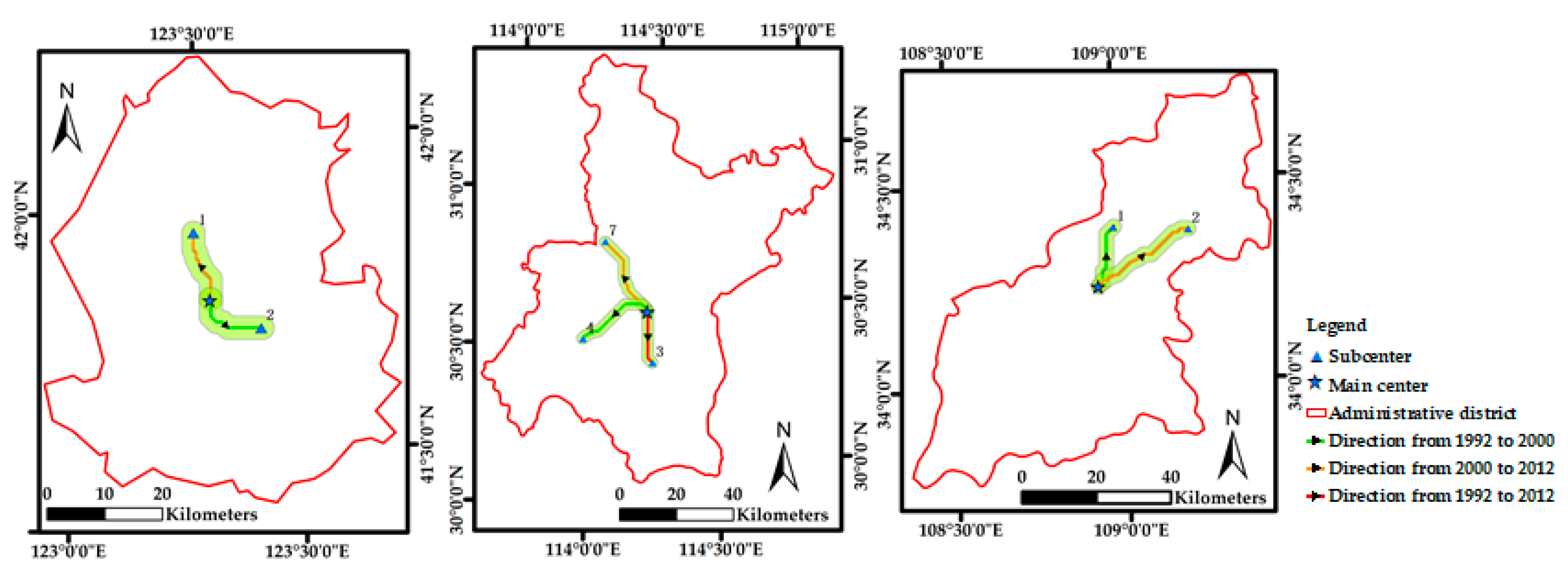
The urban expansion directions of Shenyang, Wuhan, and Xi’an are shown in Figure 13. Shenyang and Xi’an have different key spatial expansion directions from 1992 to 2000 and from 2000 to 2012. Wuhan differs from the other two cities. South of Wuhan is always the main direction, and southwest and northwest are the key directions in different periods.

4.5. Evaluation

4.5.1. Polycentric Structure Detection Accuracy

To evaluate the effectiveness of the polycentric structure definition method, the centers that are derived from the master plans for 2020 that were formulated by the governments are collected for comparison with our results. The detection accuracies for Shenyang, Wuhan, and Xi’an are listed in

Table 8. Polycentric structure detection accuracy.

Region	Center	Master Plan	Our Results	User Accuracy
Shenyang	Main centers	Heping, Shenhe, Huanggu, Dadong, Tiexi, Hunnan, Yuhong	Heping, Shenhe, Huanggu, Dadong, Tiexi, Tiexichanye b, Yuhong	81.82%
	Subcenters	Puhe, Hunhe, Tiexihchanye, Yongan	Puhe (Figure 6a, No. 1), Hunnan c (Figure 6a, No. 2)
Wuhan	Main centers	Jiangan, Jianghan, Qiaokou, Hanyang, Wuchang, Qingshan, Hongshan	Jiangan, Jianghan, Qiaokou, Hanyang, Wuchang, Qingshan, Hongshan	92.31%
	Subcenters	East, Southeast, South, Southwest, West, North	North (Figure 6b, No. 1 and No. 7), East (Figure 6b, No. 2), South (Figure 6b, No. 3), Southwest (Figure 6b, No. 4), West (Figure 6b, No. 5 and No. 6),
Xi’an	Main centers	Weiyang, Lianhu, Xincheng, Beilin, Yanta	Weiyang, Lianhu, Xincheng, Beilin, Yanta, Changning b,	66.67%
	Subcenters	Liucunpu, Changning, Xinzhu, Hongqing	Lintong a (Figure 6c, No. 1), Weiyang c (Figure 6c, No. 2)

^a Subcenters from the master plan are inconsistent with results of the proposed method; ^b Subcenters are covered by the main center region; ^c Main center is covered by the subcenter region.

. The evaluation results are described as follows:

(a) Shenyang: The main center region, which consists of seven districts (Figure 6a) that were defined by the master plan of Shenyang 2011–2020 (Shenyang Government, 2011), was detected via the proposed method.

Puhe (Figure 6a, No. 1) was detected; Tiexichanye was covered by the main center region; and Yongan and Hunhe were not detected. In addition, another subcenter (Figure 6a, No. 2), which is covered by the Hunnan district, is included in our results. The user accuracy of the method for Shenyang is 81.82%.

(b) Wuhan: The main center region consists of seven districts, as defined by the master plan of Wuhan 2010–2020 (Wuhan Government, 2011), and all of the districts were detected via the proposed method (Figure 6b). Five of the six subcenters in the master plan were detected. Panlong (Figure 6b, 1) belongs to the north, Yangluochai Lake (Figure 6b, No. 2) belongs to the east, Tangxun Lake (Figure 6b, No. 3) belongs to the south, Xuefeng (Figure 6b, No. 4) belongs to the southwest, Caidian (Figure 6b, No. 5) belongs to the west, Dongxihu (Figure 6b, No. 6) belongs to the west, and Tianhe airport (Figure 6b, No. 7) belongs to the north. Therefore, the user accuracy is 92.31%.

(c) Xi’an: The main center region of Xi’an includes five districts, as defined by the master plan of Xi’an 2008–2020 (Xi’an Government, 2009), and all of the districts were detected in this paper (Figure 6c). One subcenter (Changning) of the four subcenters that were defined by the government is covered by the main center region. As the other three subcenters have not been effectively developed (Figure 6d–f), none of them were detected. One subcenter (Figure 6c, No. 1) that was defined by the method is covered by Weiyang district, because it is close to the main center; the other subcenter is Lintong district, which is a tourist industrial zone. The user accuracy for Xi’an is 66.7%.

4.5.2. Built-Up Area Extraction Accuracy

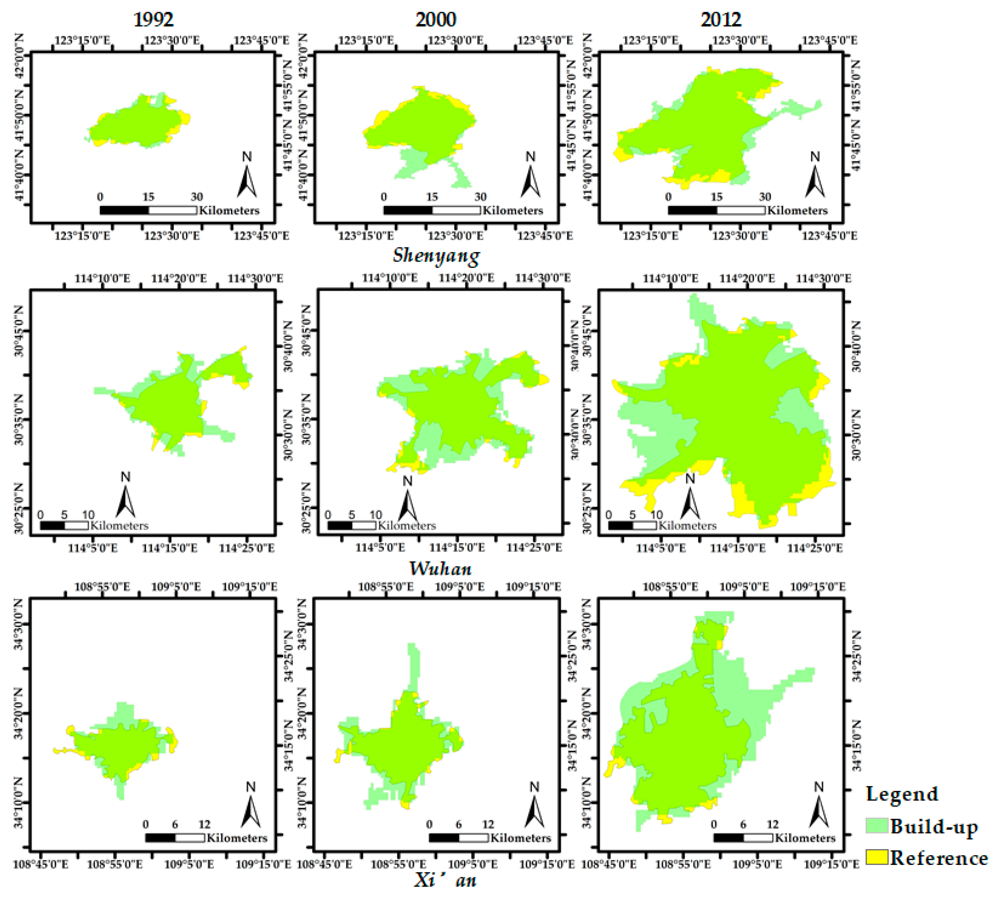
For calculating the built-up area extraction accuracy, the built-up reference areas are obtained via visual interpretation of Landsat satellite data for Shenyang, Wuhan, and Xi’an from 1992, 2000, and 2012. The built-up area reference data are shown as yellow areas in Figure 14.

(a) Shenyang. The extracted built-up areas coincide with the built-up areas of the reference data. The degree of coincidence between the built-up areas that were extracted via the proposed method and those of the reference data was gradually improved.

(b) Wuhan. The extracted built-up area covers the built-up area of the reference data as well, and the extraction result had high integrity. The number of false detections was increased compared with Shenyang. There is a large amount of water in the inner part of Wuhan, and the false detections are mostly due to the surfaces of lakes and rivers. Water-based transport and tourism industries may have caused an increase in the lighting effects in the water areas.

(c) Xi’an. The extracted built-up area matches the reference data. There are many false detections in the northeast of Xi’an, where the famous tourist district of Lintong is located. The tourist area has bright lights at night, but is covered with dense vegetation. This is an important reason why the reference data and the extracted results are not consistent. In addition, because the area that connects Lintong and the main center region has not been developed, reference data for the built-up area are not included.

The confusion matrices of the built-up area extraction accuracy for Shenyang, Wuhan, and Xi’an are presented in

Table 9. Confusion matrix for the extraction of built-up areas.

Data	Shenyang				Wuhan				Xi’an				All Mean
	1992	2000	2012	Mean	1992	2000	2012	Mean	1992	2000	2012	Mean
$A_u$	0.88	0.80	0.85	0.84	0.70	0.67	0.75	0.71	0.68	0.69	0.61	0.66	0.74
$A_m$	0.85	0.86	0.89	0.87	0.92	0.92	0.88	0.91	0.87	0.94	0.95	0.92	0.90
$A_o$	0.98	0.96	0.94	0.96	0.99	0.98	0.95	0.97	0.99	0.98	0.93	0.97	0.97
Kappa	0.86	0.81	0.84	0.84	0.79	0.76	0.78	0.78	0.76	0.78	0.70	0.75	0.79

, where the user accuracy is denoted as $A_{\mathrm{u}}$, the charting accuracy is defined as $A_m$, the overall accuracy is defined as as $A_{\mathrm{o}}$, and the Kappa coefficient is defined as Kappa.

(a) Shenyang. The mean values of $A_{\mathrm{u}}$, $A_m$, $A_{\mathrm{o}}$, and Kappa reach 0.84, 0.87, 0.96, and 0.84, respectively. There are no significant fluctuations in the indicators; hence, this method for extracting built-up areas in the region is robust.

(b) Wuhan. According to Table 9, $A_{\mathrm{u}}$ ranged from 0.67 to 0.75. The mean values of $A_{\mathrm{u}}$, $A_m$, $A_{\mathrm{o}}$, and Kappa are 0.71, 0.91, 0.97, and 0.78, respectively. The accuracy of Wuhan is lower than that of Shenyang, which may be due to the light on the rivers and lakes of Wuhan.

(c) Xi’an. The mean values of $A_m$ and $A_{\mathrm{o}}$ are 0.92 and 0.97, respectively, and both reach a more satisfactory level of accuracy. However, since the mean value of $A_{\mathrm{u}}$ is 0.66, the average value of Kappa drops to 0.75. A main reason for the decrease in the detection accuracy for Xi’an may be the light in the tourism areas on the edge of the city.

We summed all the data and calculated the mean value of each precision index. $A_m$ and $A_{\mathrm{o}}$ have ideal mean values of 0.90 and 0.97, and Kappa has a mean value of 0.79; hence, the proposed method performs well. $A_{\mathrm{u}}$ is influenced by the low radiation resolution of DMSP/OLS and natural human factors [37]; its mean value is slightly lower at 0.74. Through the above precision analysis, it is demonstrated that the method that is proposed by this paper realizes satisfactory accuracy in extracting built-up areas.

The proposed method is also compared with a built-up area extraction algorithm that is based on Iterative Self Organizing Data Analysis Techniques Algorithm(ISODATA) using DMSP/OLS data to further evaluate its reliability [38]. The accuracy of the built-up area extraction algorithm that is based on ISODATA is listed in

Table 10. Confusion matrix of the built-up area extraction method that uses ISODATA with DMSP/OLS.

Data	Shenyang				Wuhan				Xi’an				All Mean
	1992	2000	2012	Mean	1992	2000	2012	Mean	1992	2000	2012	Mean
$A_u$	0.7	0.77	0.71	0.73	0.42	0.46	0.48	0.45	0.37	0.22	0.41	0.33	0.5
$A_m$	0.95	0.94	0.98	0.96	1	1	0.99	1	0.99	1	1	1	0.99
$A_o$	0.97	0.97	0.91	0.95	0.97	0.96	0.87	0.93	0.95	0.85	0.85	0.88	0.92
Kappa	0.79	0.83	0.77	0.8	0.58	0.61	0.58	0.59	0.52	0.32	0.51	0.45	0.61

. Compared with Table 9, the $A_m$ value of the built-up area extraction algorithm that is based on ISODATA has an advantage. However, the $A_{\mathrm{u}}$ value of the built-up area extraction algorithm that is based on ISODATA is very low; hence, the results that were extracted by the algorithm have more false detections. The small value of $A_{\mathrm{u}}$ leads to decreases in the $A_{\mathrm{o}}$ and Kappa values. These results demonstrate that the proposed algorithm is more robust.

Landsat data are widely used in land-cover classification and urbanization analysis. To further analyze the reliability of the method that is proposed in this paper, we used Landsat data with the ISODATA algorithm to extract built-up areas [39]. The confusion matrix for the extraction of built-up areas based on ISODATA using Landsat data is presented in

Table 11. Confusion matrix of the built-up area extraction method that uses ISODATA with Landsat data.

Data	Shenyang				Wuhan				Xi’an				All Mean
	1992	2000	2012	Mean	1992	2000	2012	Mean	1992	2000	2012	Mean
$A_u$	0.76	0.88	0.73	0.79	0.72	0.98	0.73	0.81	0.97	0.78	0.81	0.85	0.82
$A_m$	0.83	0.67	0.75	0.75	0.43	0.69	0.87	0.66	0.61	0.87	0.85	0.78	0.73
$A_o$	0.97	0.96	0.89	0.94	0.98	0.99	0.95	0.97	0.98	0.97	0.93	0.96	0.96
Kappa	0.78	0.74	0.67	0.73	0.53	0.81	0.76	0.70	0.74	0.81	0.78	0.78	0.74

. Compared with the results in Table 9, the proposed method, which uses DMSP/OLS, and the method that uses Landsat data differ in terms of their characteristics; however, the proposed method outperforms the other method in terms of the Kappa coefficient, which reflects the overall performance of the algorithm. The results are also compared with the results that were obtained using DMSP/OLS with the same classification method of ISODATA. If the same classification algorithm is adopted, the method that uses Landsat data outperforms the method that uses DSMP/OLS data on all accuracy indices except $A_m$. The value of $A_m$ with Landsat data is relatively low; this may be because the integrity of the built-up areas that are extracted via the method that uses Landsat data is not as high compared to the method that uses DMSP/OLS data [18]. The main reason for the lower $A_{\mathrm{u}}$ of the method that uses DSMP/OLS data may be the false detections that are caused by the light spreading effect of the DMSP/OLS data [30,40]. The method that uses Landsat data realized higher accuracy due to its higher spatial resolution. According to the above comparative analysis, the proposed method effectively increased the built-up area extraction accuracy using DMSP/OLS data.

5. Discussion and Conclusions

Through the analysis of three Chinese cities, the validity of the proposed model in modeling polycentric urbanization is demonstrated. We establish the relationship between polycentric structure and urban dynamics, and detect the main urban expansion direction. To improve the precision of the built-up area extraction method that only uses spectral features, we propose a method under spatial constraints that is more robust and reliable. In contrast to the polycentric structure identification method that was proposed by [3], our method establishes the relationship between polycentric urban structure and urban dynamics to identify the key spatial expansion direction. First, the economic corridors are utilized to establish the connections between main centers and subcenters. Second, the key spatial expansion direction is identified by analyzing the multitemporal built-up area changes within the spatial buffer of each economic corridor.

5.1. Correlation Analysis of Built-Up Area and GDP

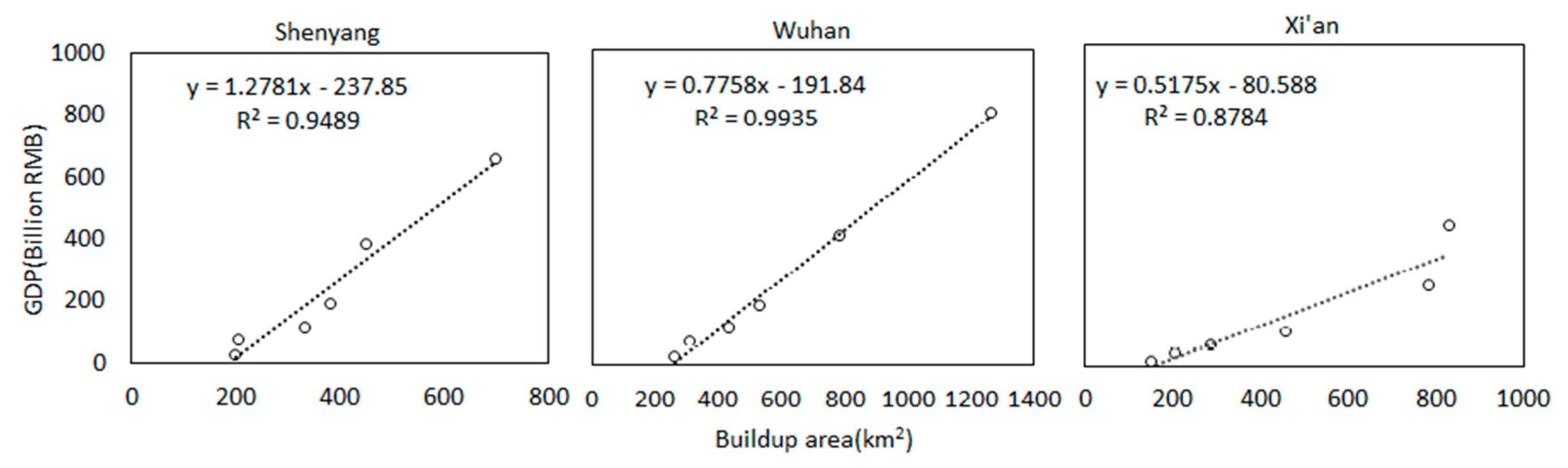
A scatter plot is used to analyze the relationship between the gross domestic product (GDP) and the built-up areas for each city in 1992, 1996, 2000, 2004, 2008, and 2012. The correlations between the built-up areas and the GDP for each city are shown in Figure 15. The R² values of the built-up areas and GDP values for Shenyang, Wuhan, and Xi’an are 0.9489, 0.9935, and 0.8784, respectively. Hence, the built-up area and GDP value have a strong positive correlation. Built-up areas can explain GDP values well.

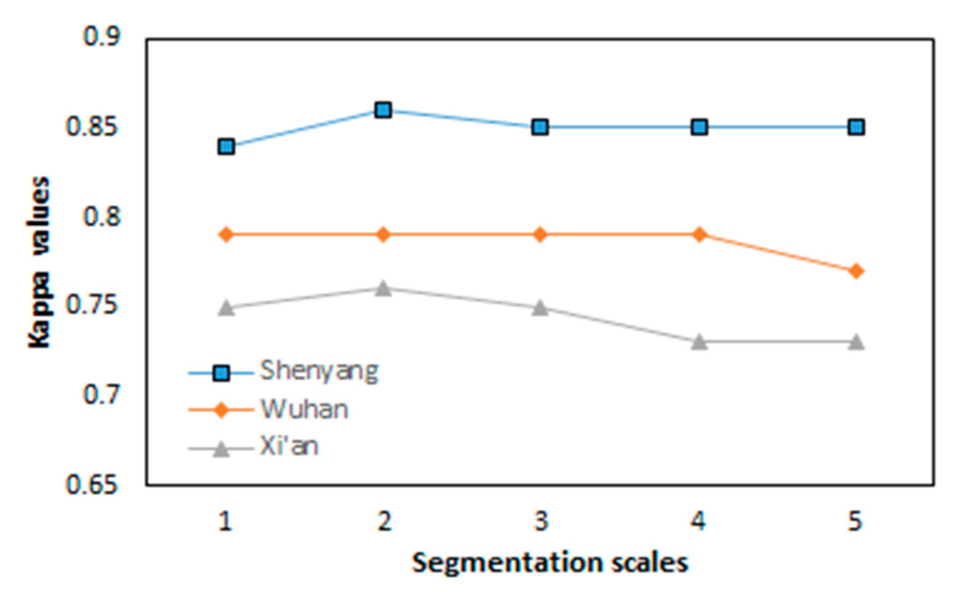
5.2. Segmentation Scale

To demonstrate the rationale behind the selection of the scale parameters, the proposed method is used to extract built-up areas with various segmentation scales. The DMSP/OLS data of Shenyang, Wuhan, and Xi’an from 1992 are selected, and the Kappa value is used as a judgment index. The segmentation scale parameters are set to one, two, three, four, and five. The relationship between the segmentation scale and the Kappa values that are obtained from the experiment is shown in Figure 15. As shown in Figure 16, the Kappa values are the highest for Shenyang and Xi’an when the segmentation scale is set to two. The Kappa values are the same for Wuhan for segmentation scales of one, two, three, and four, and the value is the lowest when the segmentation scale is five. Therefore, when the segmentation scale is set to two, the built-up area that is extracted by this method is the most accurate.

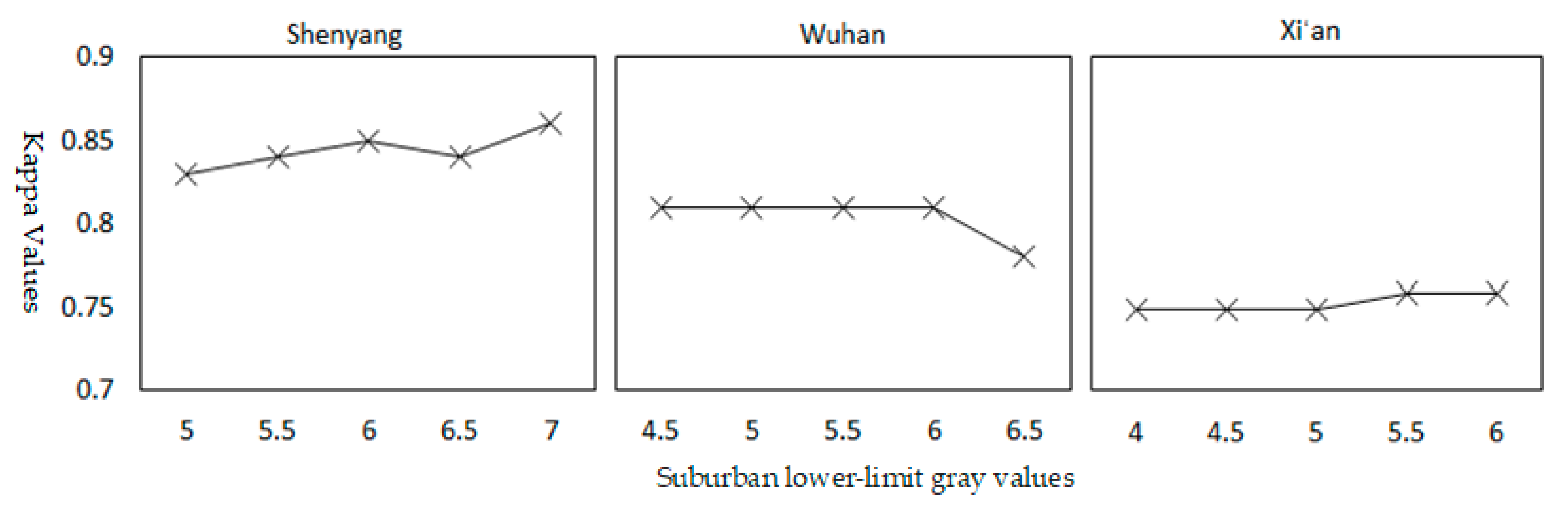
5.3. Suburban Lower-Limit Gray Value

The suburban lower-limit gray value is the maximum value at which the suburban area forms a closed ring. If the gray value exceeds the limit, the suburban ring regions will be broken. The method for analyzing the performance of various suburban lower-limit gray values is as follows: a gray value of 0.5 is selected as the step length. The analysis begins with the maximum gray value and successively decreases it four times. The DMSP/OLS data for Shenyang, Wuhan, and Xi’an from 1992 were used; the relationships between the limit gray values and the Kappa values are shown in Figure 17. The Kappa values of Shenyang and Xi’an at the extreme are the largest. The Kappa value of Wuhan decreased by 0.03 at the extreme. Hence, the suburban gray value lower-limit method is effective.

Social media data have various limitations. First, economic and cultural differences among regions will affect social media data and cause the data to differ among regions. Second, the performance of social media data varies across scales. Third, the location and content information of social media may be biased or intentionally manipulated [31]. Due to the lack of multitemporal Weibo check-in data, our model only defines the urban main center and subcenters using recent data, which might ignore changes in urban center quantity and positions.

Although the proposed built-up area extraction method has higher stability and balance than that of the previous method, the accuracy of $A_{\mathrm{u}}$ is not optimal. This finding may be due to the low data depth of the DMSP/OLS data and natural human factors. We can replace the DMSP/OLS data with VIIRS/NPP data, whose data depth is 32 bit, to improve the low radiation resolution in future research [41]. In addition, we may reduce the impact of natural human factors by using other social media data, such as POIs. Finally, we only considered human factors, not natural factors such as topological factors. Topological factors, such as ground elevation, ground slope, and ground curvature affect the distribution of the artificial facilities [42,43], which may affect the locations of built-up areas and economic corridors. Such factors should be considered in future studies. Our model can provide data support for urban management by facilitating the analysis of whether the urban development outcomes are the same as the planning intention, e.g., in terms of the main spatial expansion direction. In addition, the proposed built-up area extraction method, under spatial constraints, explicitly describes the spatial fluctuations in the magnitude of the nighttime light across the built-up areas, suburban areas, and rural areas.

References

- Friedmann, J. Four theses in the study of China’s urbanization. Int. J. Urban Regional Res. 2006, 30, 440–451. [Google Scholar] [CrossRef]
- Bai, X.; Shi, P.; Liu, Y. Society: Realizing China’s urban dream. Nat. News 2014, 509, 158. [Google Scholar] [CrossRef]
- Cai, J.; Huang, B.; Song, Y. Using multi-source geospatial big data to identify the structure of polycentric cities. Remote Sens. Environ. 2017, 202, 210–221. [Google Scholar] [CrossRef]
- McMillen, D.P. Nonparametric employment subcenter identification. J. Urban Econ. 2001, 50, 448–473. [Google Scholar] [CrossRef]
- Phelps, N.A.; Ozawa, T. Contrasts in agglomeration: proto-industrial, industrial and post-industrial forms compared. Prog. Hum. Geogr. 2003, 27, 583–604. [Google Scholar] [CrossRef]
- Banomyong, R. Benchmarking Economic Corridors logistics performance: A GMS border crossing observation. World Cust. J. 2010, 4, 29–38. [Google Scholar]
- Fernández-Maldonado, A.M.; Romein, A.; Verkoren, O.; Parente Paula Pessoa, R. Polycentric structures in Latin American metropolitan areas: Identifying employment sub-centres. Reg. Stud. 2014, 48, 1954–1971. [Google Scholar] [CrossRef]
- Liu, Z.; Liu, S. Polycentric Development and the Role of Urban Polycentric Planning in China’s Mega Cities: An Examination of Beijing’s Metropolitan Area. Sustainability 2018, 10, 1588. [Google Scholar] [CrossRef]
- Kresl, P.K. Planning Cities for the Future: The Successes and Failures of Urban Economic Strategies in Europe; Edward Elgar Publishing: Cheltenham, UK, 2015; ISBN 1847204333. [Google Scholar]
- Liu, X.; Wang, M. How polycentric is urban China and why? A case study of 318 cities. Landsc. Urban Plan. 2016, 151, 10–20. [Google Scholar] [CrossRef]
- Liu, X.; Derudder, B.; Wang, M. Polycentric urban development in China: A multi-scale analysis. Environ. Plan. B Urban Anal. City Sci. 2017. [Google Scholar] [CrossRef]
- Salvati, L.; Venanzoni, G.; Carlucci, M. Urban growth and polycentric settlements: An exploratory analysis of socioeconomic and demographic indicators in Emilia Romagna, Italy. Ital. J. Appl. Stat 2016, 26, 167–178. [Google Scholar]
- Ghosh, S.; Das, A. Exploring the lateral expansion dynamics of four metropolitan cities of India using DMSP/OLS night time image. Spat. Inf. Res. 2017, 25, 779–789. [Google Scholar] [CrossRef]
- Hausmann, A.; Toivonen, T.; Slotow, R.; Tenkanen, H.; Moilanen, A.; Heikinheimo, V.; Di Minin, E. Social Media Data Can Be Used to Understand Tourists’ Preferences for Nature-Based Experiences in Protected Areas. Conserv. Lett. 2018, 11, e12343. [Google Scholar] [CrossRef]
- Wang, R.-Q.; Mao, H.; Wang, Y.; Rae, C.; Shaw, W. Hyper-resolution monitoring of urban flooding with social media and crowdsourcing data. Comput. Geosci. 2018, 111, 139–147. [Google Scholar] [CrossRef]
- Stathakis, D.; Tselios, V.; Faraslis, I. Urbanization in European regions based on night lights. Remote Sens. Appl. Soc. Environ. 2015, 2, 26–34. [Google Scholar] [CrossRef]
- Castrence, M.; Nong, D.H.; Tran, C.C.; Young, L.; Fox, J. Mapping urban transitions using multi-temporal Landsat and DMSP-OLS night-time lights imagery of the Red River Delta in Vietnam. Land 2014, 3, 148–166. [Google Scholar] [CrossRef]
- Henderson, M.; Yeh, E.T.; Gong, P.; Elvidge, C.; Baugh, K. Validation of urban boundaries derived from global night-time satellite imagery. Int. J. Remote Sens. 2003, 24, 595–609. [Google Scholar] [CrossRef]
- Zheng, Q.; Wang, K. Analysis of the Spatio-Temporal Dynamic of Polycentric City Using Night-Time Light Remote Sensing Imagery. In Proceedings of the IGARSS 2018—2018 IEEE International Geoscience and Remote Sensing Symposium, Valencia, Spain, 22–27 July 2018. [Google Scholar]
- Chen, Z.; Yu, B.; Song, W.; Liu, H.; Wu, Q.; Shi, K.; Wu, J. A new approach for detecting urban centers and their spatial structure with nighttime light remote sensing. IEEE Trans. Geosci. Remote Sens. 2017, 55, 6305–6319. [Google Scholar] [CrossRef]
- Zhang, Q.; Schaaf, C.; Seto, K.C. The vegetation adjusted NTL urban index: A new approach to reduce saturation and increase variation in nighttime luminosity. Remote Sens. Environ. 2013, 129, 32–41. [Google Scholar] [CrossRef]
- Zhao, M.; Cheng, W.; Zhou, C.; Li, M.; Huang, K.; Wang, N. Assessing spatiotemporal characteristics of urbanization dynamics in southeast asia using time series of dmsp/ols nighttime light data. Remote Sens. 2018, 10, 47. [Google Scholar] [CrossRef]
- Li, Q.; Lu, L.; Weng, Q.; Xie, Y.; Guo, H. Monitoring urban dynamics in the southeast USA using time-series DMSP/OLS nightlight imagery. Remote Sens. 2016, 8, 578. [Google Scholar] [CrossRef]
- Kaplan, A.M.; Haenlein, M. Users of the world, unite! The challenges and opportunities of Social Media. Bus. Horiz. 2010, 53, 59–68. [Google Scholar] [CrossRef]
- Weibo reports third quarter 2015 results. Available online: http://www.nasdaq.com/press-release/weibo-reports-third-quarter-2015-results-20151118-01121 (accessed on 18 November 2015).
- He, C.; Li, J.; Chen, J.; Shi, P.; Chen, J.; Pan, Y.; Li, J.; Zhuo, L.; Toshiaki, I. The urbanization process of Bohai Rim in the 1990s by using DMSP/OLS data. J. Geogr. Sci. 2006, 16, 174–182. [Google Scholar] [CrossRef]
- Haklay, M.; Weber, P. OpenStreetMap: User-Generated Street Maps. IEEE Pervasive Comput. 2008, 7, 12–18. [Google Scholar] [CrossRef]
- Estima, J.; Painho, M. Investigating the potential of OpenStreetMap for land use/land cover production: A case study for continental Portugal, in OpenStreetMap in GIScience; Springer: Cham, Switzerland, 2015; pp. 273–293. [Google Scholar]
- Johnson, B.A.; Iizuka, K. Integrating OpenStreetMap crowdsourced data and Landsat time-series imagery for rapid land use/land cover (LULC) mapping: Case study of the Laguna de Bay area of the Philippines. Appl. Geogr. 2016, 67, 140–149. [Google Scholar] [CrossRef]
- Elvidge, C.D.; Sutton, P.C.; Baugh, K.; Ziskin, D.C.; Ghosh, T.; Anderson, S. National Trends in Satellite Observed Lighting: 1992–2009, In Global Urban Monitoring and Assessment through Earth Observation; Weng, Q., Ed.; Taylor&Fancis Group: Boca Raton, FL, USA, 2011; pp. 97–119. ISBN 9781466564503. [Google Scholar]
- Poorthuis, A.; Zook, M.; Taylor Shelton, M.G.; Stephens, M. Using Geotagged Digital Social Datain Geographic Research. In Key Methods in Geography; Clifford, N., French, S., Cope, M., Gillespie, T., Eds.; Sage: London, UK, 2016; pp. 248–269. [Google Scholar]
- Chen, Q.; Li, L.; Xu, Q.; Yang, S.; Shi, X.; Liu, X. Multi-Feature Segmentation for High-Resolution Polarimetric SAR Data Based on Fractal Net Evolution Approach. Remote Sens. 2017, 9, 570. [Google Scholar] [CrossRef]
- McMillen, D.P. Geographically Weighted Regression: The Analysis of Spatially Varying Relationships; Oxford University Press: Oxford, UK, 2004. [Google Scholar]
- Kotarba, A.Z.; Aleksandrowicz, S. Impervious surface detection with nighttime photography from the International Space Station. Remote Sens. Environ. 2016, 176, 295–307. [Google Scholar] [CrossRef]
- Kittler, J. On the accuracy of the Sobel edge detector. Image Vis. Comput. 1983, 1, 37–42. [Google Scholar] [CrossRef]
- Damania, R.; Russ, J.; Wheeler, D.; Barra, A.F. The road to growth: Measuring the tradeoffs between economic growth and ecological destruction. World Dev. 2018, 101, 351–376. [Google Scholar] [CrossRef]
- Liu, Z.; He, C.; Zhang, Q.; Huang, Q.; Yang, Y. Extracting the dynamics of urban expansion in China using DMSP-OLS nighttime light data from 1992 to 2008. Landsc. Urban Plan. 2012, 106, 62–72. [Google Scholar] [CrossRef]
- Zhang, Q.; Seto, K.C. Mapping urbanization dynamics at regional and global scales using multi-temporal DMSP/OLS nighttime light data. Remote Sens. Environ. 2011, 115, 2320–2329. [Google Scholar] [CrossRef]
- Lembani, R.L.; Knight, J.; Adam, E. Use of Landsat multi-temporal imagery to assess secondary growth Miombo woodlands in Luanshya, Zambia. South. For. J. For. Sci. 2018, 1–12. [Google Scholar] [CrossRef]
- Elvidge, C.D.; Baugh, K.E.; Dietz, J.B.; Bland, T.; Sutton, P.C.; Kroehl, H.W. Radiance calibration of DMSP-OLS low-light imaging data of human settlements. Remote Sens. Environ. 1999, 68, 77–88. [Google Scholar] [CrossRef]
- Cao, C.; Xiong, J.; Blonski, S.; Liu, Q.; Uprety, S.; Shao, X.; Bai, Y.; Weng, F. Suomi NPP VIIRS sensor data record verification, validation, and long-term performance monitoring. J. Geophys. Res. Atmos. 2013, 118, 11664–11678. [Google Scholar] [CrossRef]
- Oh, H.-J.; Kim, Y.-S.; Choi, J.-K.; Park, E.; Lee, S. GIS mapping of regional probabilistic groundwater potential in the area of Pohang City, Korea. J. Hydrol. 2011, 399, 158–172. [Google Scholar] [CrossRef]
- Lee, S.; Song, K.-Y.; Kim, Y.; Park, I. Regional groundwater productivity potential mapping using a geographic information system (GIS) based artificial neural network model. Hydrogeol. J. 2012, 20, 1511–1527. [Google Scholar] [CrossRef]
Figure 1.
Flowchart of the proposed polycentric urbanization analytical model, which uses multisource big geospatial data.
Figure 2.
Corrected multitemporal Defense Meteorological Satellite Program—Operational Linescan System (DMSP/OLS) data.
Figure 3.
Gradient images of multitemporal DMSP/OLS data.
Figure 4.
Suburban classification results.
Figure 5.
Segmentation results.
Figure 6.
Polycentric structure. (a) Shenyang; (b) Wuhan; (c) Xi’an; (d) Xinzhu; (e) Liucunpu; and (f) Hongqing; (g) North and East; (h) South, Southwest and West; (i) Puhe and Hunhan; and (j) Lintong and Weiyang.
Figure 7.
Geographically weighted regression (GWR) model.
Figure 8.
Extraction results for the built-up areas.