Estimation of Leaf Inclination Angle in Three-Dimensional Plant Images Obtained from Lidar

Graduate School, University of Tokyo, Tokyo 113-8657, Japan
*
Author to whom correspondence should be addressed.
Remote Sens. 2019, 11(3), 344; https://0-doi-org.brum.beds.ac.uk/10.3390/rs11030344
Submission received: 24 January 2019
/
Accepted: 8 February 2019
/
Published: 9 February 2019
(This article belongs to the Section Remote Sensing in Agriculture and Vegetation)
Abstract
:The leaf inclination angle is a fundamental variable for determining the plant profile. In this study, the leaf inclination angle was estimated automatically from voxel-based three-dimensional (3D) images obtained from lidar (light detection and ranging). The distribution of the leaf inclination angle within a tree was then calculated. The 3D images were first converted into voxel coordinates. Then, a plane was fitted to some voxels surrounding the point (voxel) of interest. The inclination angle and azimuth angle were obtained from the normal. The measured leaf inclination angle and its actual value were correlated and indicated a high correlation (R2 = 0.95). The absolute error of the leaf inclination angle estimation was 2.5°. Furthermore, the leaf inclination angle can be estimated even when the distance between the lidar and leaves is about 20 m. This suggests that the inclination angle estimation of leaves in a top part is reliable. Then, the leaf inclination angle distribution within a tree was calculated. The difference in the leaf inclination angle distribution between different parts within a tree was observed, and a detailed tree structural analysis was conducted. We found that this method enables accurate and efficient leaf inclination angle distribution.

1. Introduction
The leaf inclination angle is one of the most important plant structural parameters. It determines the radiation transmission within vegetation canopies [1], relates to light distribution within a canopy, affects the photosynthetic productivity of the entire plant [2,3], and helps to calculate the flux densities of radiation on leaf surfaces [4]. Moreover, it was reported that leaf inclination angle distribution should be characterized first to evaluate the leaf area index [5]. In addition, the leaf inclination angle represents plant stresses, such as water deficiency and severe heat [6,7]. Therefore, the leaf inclination angle distribution is a fundamental variable for determining the plant profile.
Owing to its importance, the leaf inclination angle has been measured with devices, such as a clinometer [8], protractor and compass [9], and three-dimensional (3D) digitizer [10,11]. Another study used a leveled digital camera, and a two-dimensional (2D) image of the target leaves was taken from the side for leaf inclination angle estimation [12]. However, with these methods, we have to measure the leaf inclination angle one by one manually, and the methods entail manual operation. Thus, the methods are very laborious and time-consuming [13]. Moreover, so many leaves (e.g., more than 100 leaves) should be tested for the inclination angle distribution of a tree and the leaves in a higher part cannot be reached. Further, the leaf inclination angle distribution exhibits a highly spatial and temporal variability [14]. Thus, a method that allows for repeatable and high-scale investigation is strongly desirable. From the reasons, the leaf inclination angle measurement with the conventional methods is not preferable in terms of its labor cost, repeatability, and scale.
A 3D scanner called lidar (light detection and ranging) provides highly accurate and dense 3D point measurements [15,16]. The lidar is very useful for the retrieval of plant structural parameters. Trunk diameter and plant height can be estimated accurately [17,18,19]. Leaf area and parameters related to leaf area can be calculated from the 3D images of plants obtained by the lidar [20,21,22,23,24]. Other than the parameters above, tree volume and species can be estimated [25,26,27]. The detailed and accurate information from lidar provides a useful tool, for example, in the field of plant phenotyping [28]. Guo et al (2018) developed a high-throughput crop phenotyping platform with lidar that can retrieve various crop structural and physiological relevant parameters efficiently [29]. For more detailed information of the lidar application for plant structural parameters, please refer to the comprehensive reviews in [30,31].
Some previous studies on leaf inclination angle estimation with 3D images are available [32,33,34,35,36,37]. In these studies, the points that composed each leaf were fitted to a plane by a least-squares method, and normals to the planes were calculated. Although this method is quite effective for leaf inclination angle estimation, each leaf should be selected manually in the 3D images one by one. Thus, exploring the distribution of the leaf inclination angle is very tedious and time-consuming. Further, owing to the manual operation, the number of leaves that can be examined is limited.
To overcome this problem, a previous study [38] converted 3D point cloud images obtained with structure from a motion method into a voxel-based 3D image. In voxel-based 3D models, a geographical space is systematically decomposed into a set of cuboid volumetric elements (voxels) [39]. Then, some voxels surrounding the point of interest are picked, and a plane fitting is performed for leaf inclination angle estimation. As a result, the leaf inclination angle can be estimated accurately. Moreover, the leaf inclination angle at each small point can be estimated, while the previous method [32,33,34,35,36,37] selected one leaf and only a representing value of the leaf inclination angle within one leaf was acquired. Although the method [39] will be useful for leaf inclination angle estimation of a target tree, this method was used only with small potted plants, and whether it is feasible to a tree remains unexplored. Thus, the accuracy of the leaf inclination angle estimation with the method should be examined.
In this study, the described method was applied to 3D images of trees obtained from lidar, and the leaf inclination angle at each small point was estimated accurately. Then, the leaf inclination angle distribution within a tree was explored.
2. Materials and Methods
2.1. Plant Material
We selected the campus of the University of Tokyo in Tokyo, Japan and the 58.3 ha Shinjuku Gyoen National Garden in Tokyo, Japan as study sites. In the campus of the University of Tokyo, there were many types of trees, such as the Himalayan cedar (Cedrus deodara), Japanese zelkova (Zelkova serrata), maidenhair tree (Ginkgo biloba), camellia (Camellia japonica), ginkgo (Ginkgo biloba L.), and sasanqua (Camellia sasanqua). The Shinjuku Gyoen National Garden has more than 10,000 trees, such as the cherry tree (Cerasus Mill.), tulip tree (Liriodendron tulipifera), plane tree (Platanus), Himalayan cedar (Cedrus deodara), Formosan sweetgum (Liquidambar formosana), and bald cypress (Taxodium distichum). These sites include a very wide variety of species; thus, we were able to select trees appropriate for the experiments. From the trees in the University of Tokyo, we selected Japanese false oak (Lithocarpus edulis), Chinese parasol tree (Firmiana simplex), Japanese Mallotus (Mallotus japonicas.), Yuzuri-ha (Daphniphyllum macropodum), and Loquat (Eriobotrya japonica). In addition, cherry blossoms (Cerasus Mill.) and Japanese Aucuba (Aucuba japonica) in Shinjuku Gyoen National Garden were selected for the experiments. The target trees were far from neighboring trees so that their images could be obtained without the interference from their leaves and branches.
2.2. Lidar Measurement
Lidar is a laser-based instrument that measures its surroundings for range measurement and precise angular measurements through an optical beam deflection mechanism to derive 3D point observations from the object surfaces [40,41]. The lidar used in this study was the Focus3D X330 (FARO, Florida, USA). The FARO Focus3D X 330 laser scanner has a vertical field of view of 300° and a maximum vertical scan speed of 97 Hz. Its measurement speed ranges from 122 to 976 kpts/s. The scan range is 0.6 m to 330 m, and its weight is 5.2 kg [42]. The lidar was attached to a tripod whose height was about 1.5 m. Parameters called “resolution” and “quality” have to be set for the lidar measurements. Then, “point distance at 10 m” and time for the measurement are determined. The values of resolution and quality were set around 1/2 to 1/4 and 4, which are corresponding to “high” in the available range from “low” to “very high”. The point distance at 10 m and time for the measurement are about 3 to 6 mm at 10 m and 10 minutes. A point pre-processing for the estimation was not done due to the precise 3D reconstruction of the lidar. The measurement was conducted on a windless day without rainfall.
2.3. Leaf Inclination Angle Estimation
For leaf inclination angle estimation, first, the 3D point cloud images were converted into voxel coordinates. In the construction of voxel-based 3D images, the X, Y, and Z values of each point in the 3D point cloud images were rounded to the nearest integer value; this leads to the efficient calculation of the structural parameters [18,19]. The distance to the neighboring point corresponds to voxel size in the voxel-coordinate. The voxel size was set at around 0.5 cm. Voxels corresponding to coordinates converted from points within the data were assigned an attribute value of 1, and the attribute value of vacant voxels was set as zero [26]. To estimate the leaf inclination angle, a plane was fitted around a voxel and all voxels with an attribute value of 1 among the 342 neighboring voxels (7 × 7 × 7 − 1) around the point (voxel) of interest as shown in Figure 1. This calculation was performed throughout the voxels with an attribute value of 1 in the 3D image. Then, the zenith angle and azimuth angle of a vector normal to the fitted plane were calculated. From the normal, the leaf inclination angle and azimuth angle were estimated. The zenith angle corresponds to the leaf inclination angle [38]. The leaf inclination angle estimation was conducted at each voxel of the leaves, meaning the plane fitting was conducted to each voxel of the leaves. Thus, this method does not entail any manual operations. After this estimation, its accuracy was validated; then, a distribution of leaf inclination angle within a tree was calculated. The flow is shown in Figure 2.
2.3.1. Evaluation of Leaf Inclination Angle Estimation Accuracy
To evaluate the leaf inclination angle estimation accuracy, we randomly selected points from the voxels constituting the leaves in the 3D images (n = 35). The actual inclination angle of these points was measured manually using an inclinometer. We conducted the manual measurement on a stage, ladder or box when the target leaf was located in a higher space, and we did not take off the leaf. Then, we compared the estimated values with the actual values.
2.3.2. Relationship between Distance from Lidar to Leaves and Leaf Inclination Angle Estimation Accuracy
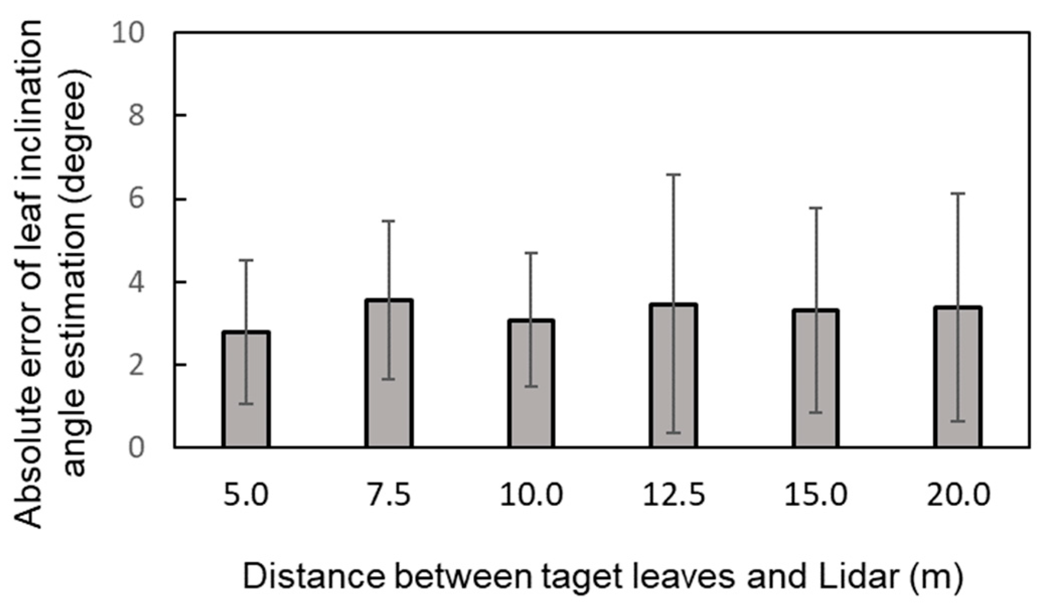
As the distance between the lidar to the leaves increases, the resolution of the 3D image decreases, resulting in an estimation error of the tree structural parameters [43]. However, the lidar used in this study offers 3D images with very high resolution; hence, the distance might not significantly affect the estimation accuracy. In a lidar measurement, when the target tree is tall, the distance between the lidar and each part of the tree differs significantly. Then, the distance dependence in the leaf inclination angle estimation should be investigated.
2.3.3. Relationship between Length of One Side of Plane for Fitting and Leaf Inclination Angle Estimation Accuracy
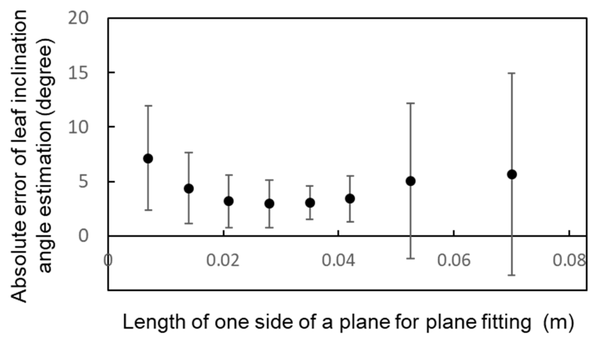
In leaf inclination angle estimation, the points used for the plane fitting will affect the estimation accuracy. As mentioned above, the neighboring 342 voxels (7 × 7 × 7 − 1) around the point (voxel) of interest were used for the plane fitting. Here, the voxel size (i.e., the length of one side of a voxel) was changed, and its estimation accuracy was investigated with Yuzuri-ha. The length of one side of the plane for fitting was obtained by multiplying the voxel size by 7 (i.e., the number of voxels of one side of a plane). To change the length of one side of the planes, it is also possible to change the number of points to be used instead of the voxel size. Here, the result is not significantly different when changing the number to that obtained when changing the voxel size. Thus, here, only the voxel size was changed.
2.3.4. Difference of Leaf Inclination Angle Distribution within a Tree
For the Japanese false oak and Chinese parasol tree, the leaf inclination angles at the top part and lower part were calculated, and these distributions were obtained with histograms. Then, the difference in the leaf inclination angle distribution between the top and lower parts of the tree was observed. In addition, using Japanese Mallotus, the leaf inclination angle distribution was determined. The leaves in the lower part started to become yellowish (i.e., non-green). Non-green areas, that is, all areas with a normalized green value [G/(R + G + B)] of less than 0.4 were classified into one part. The green areas were classified into the other part. Then, the difference between the leaf inclination angle distributions in the green and non-green parts was compared.
For cherry blossom and Japanese Aucuba, the leaf inclination angle distribution within the tree was calculated. For Japanese Aucuba, the distribution of the azimuth angle was estimated.
3. Results and Discussion
3.1. Evaluation of Leaf Inclination Angle Estimation Accuracy
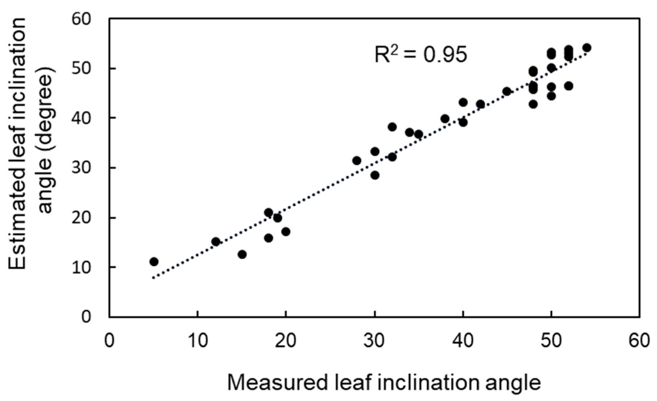
Figure 3 shows the relationship between the measured leaf inclination angle and the estimated leaf inclination angle. The relationship indicates a high correlation (R2 = 0.95). The absolute error was 2.5°, and the accuracy was as high as that obtained manually [3]. This indicates that the leaf inclination angle can be estimated accurately. The high accuracy comes from the appropriate selection of voxels for plane fitting. In this study, voxels with an attribute value of 1 in the neighboring 342 points were used for the fitting. The reconstructed 3D images obtained by lidar were precise, and the number of points was sufficient. Thus, the leaf normal represented the leaf inclination angle. The calculation with the voxel-based 3D images can be conducted swiftly, while the calculation with the 3D point cloud takes longer.
3.2. Relationship between Distance from Lidar to Leaves and Leaf Inclination Angle Estimation
Figure 4 shows the relationship between the distance to the target leaves from the lidar and the absolute error of the leaf inclination angle estimation. The absolute estimation error varies from 2.0° to 4.0° at each distance. There is no significant difference between them. As the distance increases, the resolution of the 3D images decreases. However, the lidar used in this study offers 3D images with high resolution. As a result, the accuracy remains good even when the distance increases. Then, even when observing a tall tree, that is, when the distance between the leaves and lidar is comparatively far (e.g., 15 m), the leaf inclination angle estimation of the leaves in a higher part is accurate and reliable. The accuracy is influenced by the resolution of the obtained 3D point cloud images, so a higher resolution (e.g., the distance to the neighboring point: 0.5 cm) is desirable.
3.3. Relationship between Length of One Side of Plane for Fitting and Leaf Inclination Angle Estimation
Figure 5 illustrates the relationship between the length of one side of a plane for plane fitting and the absolute error of the leaf inclination angle estimation. When the length is about 0.02 to 0.05 m, it reaches its minimum. When the length is shorter (e.g., 0.01 m) or longer (e.g., 0.07 m), the error increases.
If the length is shorter, that is, the plane is smaller, the fitting is influenced by noises on the leaf surface or the localization errors of points. As a result, a normal that represents the leaf orientation in a small area cannot be created. On the other hand, if the length of one side of a plane is longer, the estimated value shows the representative value of one leaf or a large part within the leaf. The inclination angle differs within one leaf, so fitting with a large plane leads to an increased estimation error.
When using a large plane and a target point located near the leaf edges, the plane fitting is conducted with points in neighboring leaves. This also leads to an estimation error. This error occurs when the leaves are close to each other, and the distance is shorter than the length of one side of the plane. In this study, this kind of error did not occur; however, when the target leaves are heavily overlapped, this kind of error will occur.
The determination of the size of the plane even when we do not use voxel-based coordinates is inevitable. However, when setting the length of one side of a plane from 1 cm to 5 cm, the kinds of errors mentioned in the last paragraph were not observed. The acceptable range of the length is comparatively wide, and the length can be set around 3 cm.
As another method for leaf inclination angle estimation, a small surface was created with two neighboring points, and a normal on the triangle was calculated. Then, the leaf inclination angle was estimated from the normal [44]. However, the normal tends to be influenced by noises or incorrect localizations of points, resulting in comparatively low accuracy. This corresponds to the case where the length of one side of a plane for fitting is set as short as possible, and the error increases as the length becomes shorter, as shown in Figure 5.
In this study, voxel-based 3D images were used, and their X, Y, and Z values were converted into nearest-integer values. The 3D images had high resolution, so we were not concerned about a decrease in the resolution of the 3D images owing to the voxelization, and the plane fitting could be done precisely. Moreover, owing to the high resolution, many points could be found in a small region. If the resolution is not sufficient, three points cannot be found near the point of interest, plane fitting cannot be accomplished. However, in this study, such cases did not occur, which means the leaf inclination angle estimation from the 3D images obtained by lidar with this method is robust and reliable.
3.4. Difference of Leaf Inclination Angle Distribution within a Tree
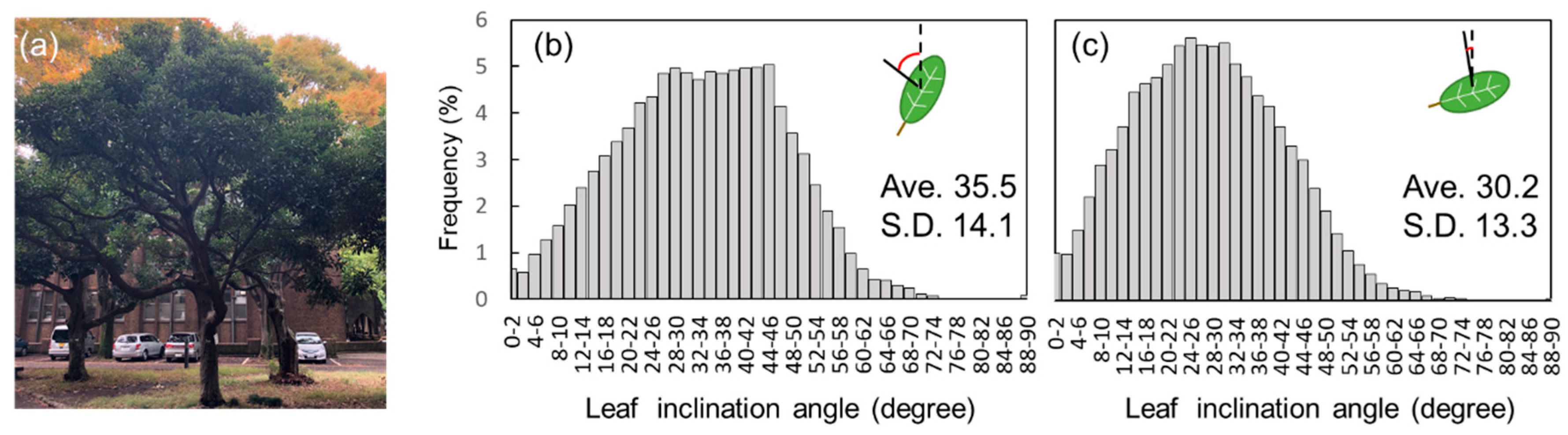
Figure 6a shows the leaf inclination distribution of Japanese false oak at higher and lower parts. The leaves in a top part tend to “stand up,” and the leaves in a lower part tend to “lie,” as shown in Figure 6b,c. The average inclination angles for the top part and lower part were 35.5° and 30.2°, respectively. Adjusting the leaf inclination angle distribution to improve the transmission of light through the canopy provides an important way to maximize the light availability throughout the entire vertical profile of the plant canopy [45,46]. It is suggested that to let sunlight into the inside canopy, the leaves in the top part are greatly inclined [46,47]. In addition to the light reception, owing to the steepness, the Japanese false oak can accept much more water from rainfall [48]. On the other hand, to obtain the sunlight, leaves in the lower part are comparatively parallel to the ground.
By contrast, the leaves are parallel to the ground in the top part (Figure 7b), and those in the lower part are inclined (Figure 7c) in a Chinese parasol tree. This implies that to obtain sunlight at its maximum, the leaves in the top part are parallel to the ground. On the other hand, to obtain scattered light, leaves in the lower part are inclined. This tendency is opposite to that of the Japanese false oak.
The distribution is also affected by other factors. For example, the distribution changes to escape heat stress [49,50,51]. By letting the leaves be significantly inclined, the light reception can be decreased; accordingly, the decreasing of the light reception can alleviate the heat stress on the leaf. The leaf inclination angle distribution determined based on the strategy for these optimizations is different one by one. This method offers leaf inclination angle distribution accurately and automatically. It can be a very effective tool for understanding the mechanisms of adaptation to ambient factors.
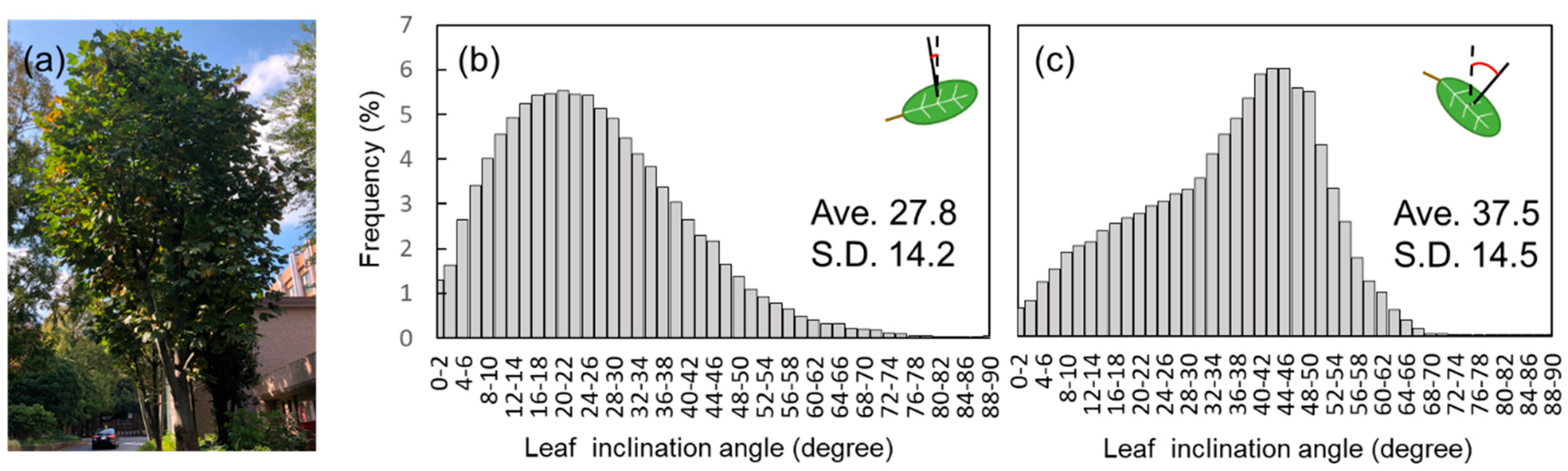
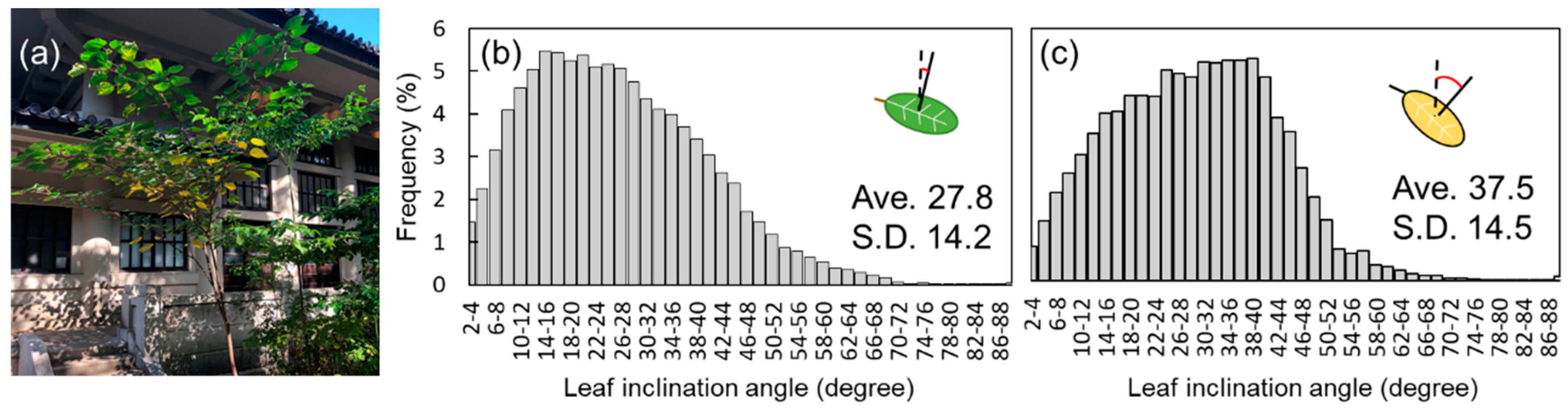
Figure 8a shows an image of the Japanese Mallotus, and histograms (b) and (c) show the inclination angle distribution of the green and yellow parts, respectively. The yellow-colored leaves are mainly located at the lower part of the tree. In a Japanese Mallotus, as it becomes yellowish, it becomes inclined; accordingly, the peak shifts to the right. The averages in the top and lower parts were 27.8° and 37.5°, respectively.
Many leaves become inclined before its senescence. In this sample, leaves become yellowish before falling down, so color information helps to evaluate the extent of the senescence. However, when the target leaves do not have a significant color change before senescence, observation of the leaf inclination angle might be useful for evaluating the plant status. Furthermore, the inclination of other types of organs, such as stems and ears, affects the light environment of the canopy [3], so observation of these parts also leads to a deep understanding of plant ecology.
3.5. Leaf Inclination Angle Distribution within a Tree
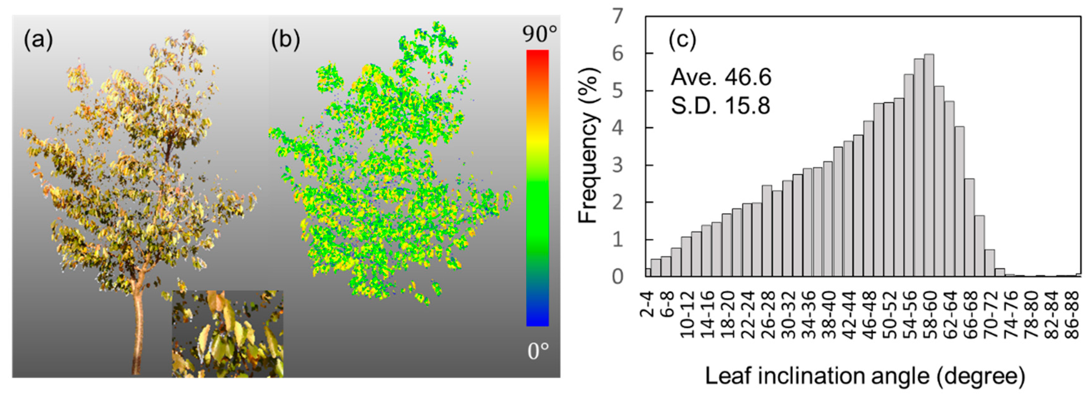
With this method, the leaf inclination angle in each small area can be estimated, which leads to a distribution map. Figure 9a,b show the original 3D image and its leaf inclination angle map of a cherry blossom, respectively. Here, branches were cut manually. From (b), the distribution can be listed in the histogram shown in Figure 9c. The average and standard deviation are 46.6 and 15.8°, respectively. Figure 9a,b also show the original 3D image and its leaf inclination angle map (Japanese Aucuba).
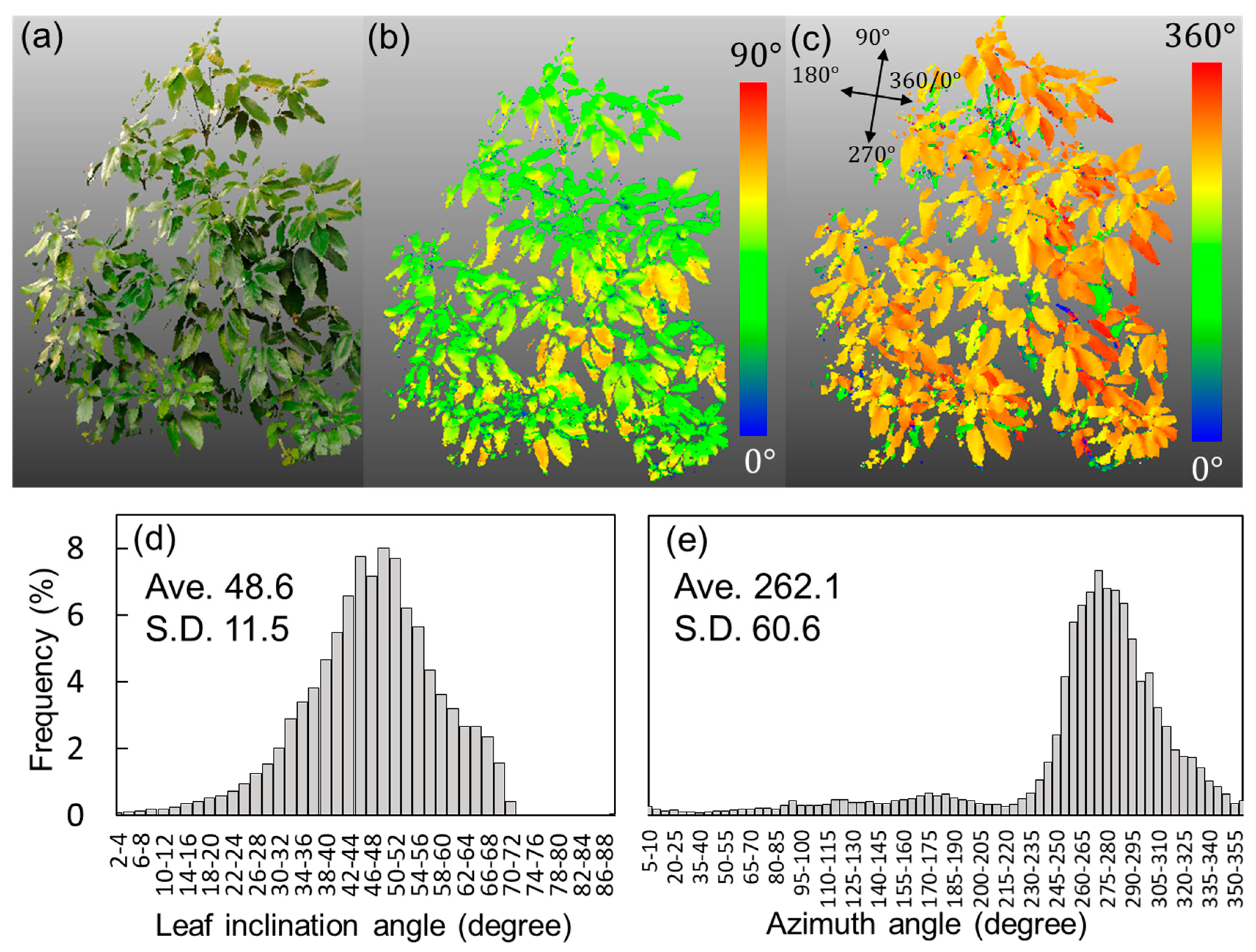
Figure 10c shows the azimuth angle distribution. Histograms of the leaf inclination angle and azimuth angle distribution are shown in Figure 10d,e, respectively. The average values (standard deviations) are 48.6 (11.5) and 262.1° (60.6°), respectively. The difference in the distribution comes, for example, from the light and heat conditions, as mentioned. The locations and structures of the neighboring trees and objects affect the light condition of the target tree. The light condition is difficult to predict considering the environment around the sample with a mathematical model. However, it is possible to predict the light condition using 3D images including other objects, such as when using ray tracing.
Stomatal conductance is a very important parameter in understanding the process of exchanging carbon dioxide, water, vapor, and heat between plants and the atmosphere [52]. To predict the stomatal conductance, the quantity of heat from the light reception should be calculated. For this calculation, the leaf inclination angle distribution is needed [53]. Some models for the stomatal conductance considering the leaf inclination angle have been proposed [54,55]. Thanks to the automatic acquisition of the angle distribution, this method also contributes to the evaluation and implementation of these models.
4. Conclusions
In this study, the leaf inclination angle was automatically estimated from voxel-based three-dimensional (3D) images obtained from lidar. Then, the distribution of the leaf inclination angle within a tree was calculated. The measured leaf inclination angle and its actual value were correlated and indicated a high correlation (R2 = 0.95). The absolute error of the leaf inclination angle estimation was 2.5°.
It was found that even when the distance between the lidar and target leaves was great (e.g., 20 m), the leaf inclination angle estimation could be done accurately. This suggests that the angle in a top part of a tree can be estimated well. In addition, when the length of one side of a plane for fitting is about 2.0 to 5.0 cm, the estimation can be done accurately. In a future work, the inclination angle estimation of a leaf that locates in a higher place should be directly investigated.
Then, the leaf inclination angle distribution was calculated within one leaf. The difference in the leaf inclination angle distribution was observed between a top part and lower part of a tree. The distribution at each part was determined by many factors, such as the light–heat condition. Previously, investigating the leaf angle was tedious and time-consuming. However, the method proposed here allows for automatic and accurate leaf inclination estimation.
This method is especially effective when a large-scale measurement or time-series measurement are necessary. Therefore, it is expected that this method will be applied in a wide variety of fields and objectives, and will help in understanding the mechanisms of the adaptation of plants to the ambient environment.
Author Contributions
K.I. conducted the experiment and analysis. This paper was written by K.I. F.H. supervised this research.
Funding
This work was supported by ACT-I, Japan Science and Technology Agency (Grant number: JPMJPR18U4).
Conflicts of Interest
The authors declare no conflict of interest.
References
- Pisek, J.; Sonnentag, O.; Richardson, A.D.; Mõttus, M. Is the spherical leaf inclination angle distribution a valid assumption for temperate and boreal broadleaf tree species? Agric. Fore. Meteorol. 2013, 169, 186–194. [Google Scholar] [CrossRef]
- Kishitani, S.; Takano, Y.; Tsunoda, S. Optimum leaf-areal nitrogen content of single leaves for maximizing the photosynthesis rate of leaf canopies: A simulatron in rice. Jap. J. Breeding 1972, 22, 1–10. [Google Scholar] [CrossRef]
- Hosoi, F.; Nakai, Y.; Omasa, K. Estimating the leaf inclination angle distribution of the wheat canopy using a portable scanning lidar. J. Agric. Meteol. 2009, 65, 297–302. [Google Scholar] [CrossRef] [Green Version]
- Falster, D.S.; Westoby, M. Leaf size and angle vary widely across species: What consequences for light interception? New Phytol. 2003, 158, 509–525. [Google Scholar] [CrossRef]
- Ryu, Y.; Sonnentag, O.; Nilson, T.; Vargas, R.; Kobayashi, H.; Wenk, R.; Baldocchi, D.D. How to quantify tree leaf area index in an open savanna ecosystem: A multi-instrument and multi-model approach. Agric. Fore. Meteorol. 2010, 150, 63–76. [Google Scholar] [CrossRef]
- Omasa, K.; Hosoi, F.; Konishi, A. 3D lidar imaging for detecting and understanding plant responses and canopy structure. J. Exp. Bot. 2006, 58, 881–898. [Google Scholar] [CrossRef] [Green Version]
- Konishi, A.; Eguchi, A.; Hosoi, F.; Omasa, K. 3D monitoring spatio–temporal effects of herbicide on a whole plant using combined range and chlorophyll a fluorescence imaging. Funct. Plant Biol. 2009, 36, 874–879. [Google Scholar] [CrossRef]
- Gratani, L.; Ghia, E. Changes in morphological and physiological traits during leaf expansion of Arbutus unedo. Environ. Exp. Bot. 2002, 48, 51–60. [Google Scholar] [CrossRef]
- Norman, J.M.; Campbell, G.S. Canopy structure. In Plant Physiological Ecology; Springer: Berlin, Germany, 1989; pp. 301–325. [Google Scholar]
- Sinoquet, H.; Thanisawanyangkura, S.; Mabrouk, H.; Kasemsap, P. Characterization of the light environment in canopies using 3D digitising and image processing. Ann. Bot. 1998, 82, 203–212. [Google Scholar] [CrossRef]
- Shono, H. A new method of image measurement of leaf tip angle based on textural feature and a study of its availability. Environ. control boil. 1995, 33, 197–207. [Google Scholar] [CrossRef]
- Pisek, J.; Ryu, Y.; Alikas, K. Estimating leaf inclination and G-function from leveled digital camera photography in broadleaf canopies. Trees 2011, 25, 919–924. [Google Scholar] [CrossRef]
- Honjo, T.; Shono, H.; Takatsuji, M. Measurement and visualizatioonf plant shape. SHITA J. 1993, 4, 151–156. [Google Scholar]
- Wang, W.M.; Li, Z.L.; Su, H.B. Comparison of leaf angle distribution functions: Effects on extinction coefficient and fraction of sunlit foliage. Agric. Fore. Meteorol. 2007, 143, 106–122. [Google Scholar] [CrossRef] [Green Version]
- Milenković, M.; Ressl, C.; Karel, W.; Mandlburger, G.; Pfeifer, N. Roughness Spectra Derived from Multi-Scale LiDAR Point Clouds of a Gravel Surface: A Comparison and Sensitivity Analysis. ISPRS Int. J. Geo-Inf. 2018, 7, 69. [Google Scholar] [CrossRef]
- Xing, X.-F.; Mostafavi, M.-A.; Chavoshi, S.H. A Knowledge Base for Automatic Feature Recognition from Point Clouds in an Urban Scene. ISPRS Int. J. Geo-Info. 2018, 7, 28. [Google Scholar] [CrossRef]
- Chen, C.; Wang, Y.; Li, Y.; Yue, T.; Wang, X. Robust and Parameter-Free Algorithm for Constructing Pit-Free Canopy Height Models. ISPRS Int. J. Geo-Info. 2017, 6, 219. [Google Scholar] [CrossRef]
- Yuan, W.; Li, J.; Bhatta, M.; Shi, Y.; Baenziger, P.; Ge, Y. Wheat height estimation using LiDAR in comparison to ultrasonic sensor and UAS. Sensors 2018, 18, 3731. [Google Scholar] [CrossRef]
- Itakura, K.; Hosoi, F. Automatic individual tree detection and canopy segmentation from three-dimensional point cloud images obtained from ground-based lidar. J. Agric. Meteol. 2018, 74, 109–113. [Google Scholar] [CrossRef]
- Hosoi, F.; Omasa, K. Voxel-based 3-D modeling of individual trees for estimating leaf area density using high-resolution portable scanning lidar. IEEE Trans. Geosci. Remote Sens. 2006, 44, 3610–3618. [Google Scholar] [CrossRef]
- Hosoi, F.; Omasa, K. Estimating vertical plant area density profile and growth parameters of a wheat canopy at different growth stages using three-dimensional portable lidar imaging. ISPRS J. Photogramm. Remote Sens. 2009, 64, 151–158. [Google Scholar] [CrossRef]
- Hosoi, F.; Nakai, Y.; Omasa, K. Estimation and error analysis of woody canopy leaf area density profiles using 3-D airborne and ground-based scanning lidar remote-sensing techniques. IEEE Trans. Geosci. Remote Sens. 2010, 48, 2215–2223. [Google Scholar] [CrossRef]
- Hosoi, F.; Nakabayashi, K.; Omasa, K. 3-D modeling of tomato canopies using a high-resolution portable scanning lidar for extracting structural information. Sensors 2011, 11, 2166–2174. [Google Scholar] [CrossRef] [PubMed]
- Hu, R.; Bournez, E.; Cheng, S.; Jiang, H.; Nerry, F.; Landes, T.; Saudreau, M.; Kastendeuch, P.; Najjar, G.; Colin, J. Estimating the leaf area of an individual tree in urban areas using terrestrial laser scanner and path length distribution model. ISPRS J. Photogramm. Remote Sens. 2018, 144, 357–368. [Google Scholar] [CrossRef]
- Shi, Y.; Wang, T.; Skidmore, A.K.; Heurich, M. Important LiDAR metrics for discriminating forest tree species in Central Europe. ISPRS J. Photogramm. Remote Sens. 2018, 137, 163–174. [Google Scholar] [CrossRef]
- Hosoi, F.; Nakai, Y.; Omasa, K. 3-D voxel-based solid modeling of a broad-leaved tree for accurate volume estimation using portable scanning lidar. ISPRS J. Photogramm. Remote Sens. 2013, 82, 41–48. [Google Scholar] [CrossRef]
- Pérez-Ruiz, M.; Rallo, P.; Jiménez, M.R.; Garrido-Izard, M.; Suárez, M.P.; Casanova, L.; Valero, C.; Martínez-Guanter, J.; Morales-Sillero, A. Evaluation of over-the-row harvester damage in a super-high-density olive orchard using on-board sensing techniques. Sensors 2018, 18, 1242. [Google Scholar] [CrossRef] [PubMed]
- Thapa, S.; Zhu, F.; Walia, H.; Yu, H.; Ge, Y. A novel LiDAR-based instrument for high-throughput, 3D measurement of morphological traits in maize and sorghum. Sensors 2018, 18, 1187. [Google Scholar] [CrossRef]
- Guo, Q.; Wu, F.; Pang, S.; Zhao, X.; Chen, L.; Liu, J.; Xue, B.; Xu, G.; Li, L.; Jing, H. Crop 3D—A LiDAR based platform for 3D high-throughput crop phenotyping. Sci. China Life Sci. 2018, 61, 328–339. [Google Scholar] [CrossRef]
- Leeuwen, M.V.; Nieuwenhuis, M. Retrieval of forest structural parameters using LiDAR remote sensing. Eur. J. For. Res. 2010, 129, 749–770. [Google Scholar] [CrossRef]
- Dassot, M.; Constant, T.; Fournierl, M. The use of terrestrial LiDAR technology in forest science: application fields, benefits and challenges. Ann. For. Sci. 2011, 68, 959–974. [Google Scholar] [CrossRef]
- Hosoi, F.; Omasa, K. Factors contributing to accuracy in the estimation of the woody canopy leaf area density profile using 3D portable lidar imaging. J. Exp. Bot. 2007, 58, 3463–3473. [Google Scholar] [CrossRef] [PubMed] [Green Version]
- Hosoi, F.; Omasa, K. Detecting seasonal change of broad-leaved woody canopy leaf area density profile using 3D portable LIDAR imaging. Funct. Plant Biol. 2009, 36, 998–1005. [Google Scholar] [CrossRef]
- Hosoi, F.; Omasa, K. Estimation of vertical plant area density profiles in a rice canopy at different growth stages by high-resolution portable scanning lidar with a lightweight mirror. ISPRS J. Photogramm. Remote Sens. 2012, 74, 11–19. [Google Scholar] [CrossRef]
- Hosoi, F.; Omasa, K. Estimating leaf inclination angle distribution of broad-leaved trees in each part of the canopies by a high-resolution portable scanning lidar. J. Agric. Meteorol. 2015, 71, 136–141. [Google Scholar] [CrossRef] [Green Version]
- Mizuki, S.; Hosoi, F.; Omasa, K. Measurement of seasonal change of leaf inclination angle distributions in ginkgo trees using a high resolution portable scanning lidar. Eco Eng. 2015, 27, 99–103. [Google Scholar]
- Blomley, R.; Hovi, A.; Weinmann, M.; Hinz, S.; Korpela, I.; Jutzi, B. Tree species classification using within crown localization of waveform LiDAR attributes. ISPRS J. Photogramm. Remote Sens. 2017, 133, 142–156. [Google Scholar] [CrossRef]
- Itakura, K.; Hosoi, F. Automatic leaf segmentation for estimating leaf area and leaf inclination angle in 3D plant images. Sensors 2018, 18, 3576. [Google Scholar] [CrossRef]
- Wu, B.; Yu, B.; Yue, W.; Shu, S.; Tan, W.; Hu, C.; Huang, Y.; Wu, J.; Liu, H. A voxel-based method for automated identification and morphological parameters estimation of individual street trees from mobile laser scanning data. Remote Sens. 2013, 5, 584–611. [Google Scholar] [CrossRef]
- Liang, X.; Kankare, V.; Hyyppä, J.; Wang, Y.; Kukko, A.; Haggrén, H.; Yu, X.; Kaartinen, H.; Jaakkola, A.; Guan, F. Terrestrial laser scanning in forest inventories. ISPRS J. Photogramm. Remote Sens. 2016, 115, 63–77. [Google Scholar] [CrossRef] [Green Version]
- Soma, M.; Pimont, F.; Durrieu, S.; Dupuy, J.-L. Enhanced Measurements of Leaf Area Density with T-LiDAR: Evaluating and Calibrating the Effects of Vegetation Heterogeneity and Scanner Properties. Remote Sens. 2018, 10, 1580. [Google Scholar] [CrossRef]
- Faro. FARO Laser Scanner Focus 3D X 330—The Perfect Instrument for 3D Documentation and Land Surveying. 2014. Available online: http://www.iqlaser.co.za/files/04ref201-519-en---faro-laserscanner-focus3d-x-330-tech-sheet.pdf (accessed on 22 September 2014).
- Itakura, K.; Kamakura, I.; Hosoi, F. A Comparison study on three-dimensional measurement of vegetation using lidar and SfM on the ground. Eco Eng. 2018, 30, 15–20. [Google Scholar]
- Bailey, B.N.; Mahaffee, W.F. Rapid measurement of the three-dimensional distribution of leaf orientation and the leaf angle probability density function using terrestrial LiDAR scanning. Remote Sens. Environ. 2017, 194, 63–76. [Google Scholar] [CrossRef]
- Raabe, K.; Pisek, J.; Sonnentag, O.; Annuk, K. Variations of leaf inclination angle distribution with height over the growing season and light exposure for eight broadleaf tree species. Agric. Forest Meteorol. 2015, 214, 2–11. [Google Scholar] [CrossRef]
- Niinemets, Ü. A review of light interception in plant stands from leaf to canopy in different plant functional types and in species with varying shade tolerance. Ecol. Res. 2010, 25, 693–714. [Google Scholar] [CrossRef]
- Utsugi, H.; Araki, M.; Kawasaki, T.; Ishizuka, M. Vertical distributions of leaf area and inclination angle, and their relationship in a 46-year-old Chamaecyparis obtusa stand. Forest Ecol. Manag. 2006, 225, 104–112. [Google Scholar] [CrossRef]
- Sato, Y.; Inokura, Y.; Osaki, S.; Sugihara, S.; Yoshimura, K.; Ogawa, S. Comparison of water chemistry in throughfall and stem flow between two species with different crown structure. Bull. Kyushu Univ. For. 1997, 77, 13–24. [Google Scholar]
- Muraoka, H.; Takenaka, A.; Tang, Y.; Koizumi, H.; Washitani, I. Flexible leaf orientations of Arisaema heterophyllum maximize light capture in a forest understorey and avoid excess irradiance at a deforested site. Ann. Bot. 1998, 82, 297–307. [Google Scholar] [CrossRef]
- Ball, M.; Cowan, I.R.; Farquhar, G.D. Maintenance of leaf temperature and the optimisation of carbon gain in relation to water loss in a tropical mangrove forest. Funct. Plant Biol. 1988, 15, 263–276. [Google Scholar] [CrossRef]
- Medina, E.; Sobrado, M.; Herrera, R. Significance of leaf orientation for leaf temperature in an Amazonian sclerophyll vegetation. Rad. Environ. Biophys. 1978, 15, 131–140. [Google Scholar] [CrossRef]
- Farquhar, G.D.; Sharkey, T.D. Stomatal conductance and photosynthesis. Ann. Rev. Plant Physiol. 1982, 33, 317–345. [Google Scholar] [CrossRef]
- Detto, M.; Asner, G.P.; Muller-Landau, H.C.; Sonnentag, O. Spatial variability in tropical forest leaf area density from multireturn lidar and modeling. J. Geophys. Res. Biogeosci. 2015, 120, 294–309. [Google Scholar] [CrossRef] [Green Version]
- Sellers, P.J. Canopy reflectance, photosynthesis and transpiration. Int. J. Remote Sens. 1985, 6, 1335–1372. [Google Scholar] [CrossRef] [Green Version]
- Sellers, P.J.; Mintz, Y.; Sud, Y.C.E.A.; Dalcher, A. A simple biosphere model (SiB) for use within general circulation models. J. Atmosph. Sci. 1986, 43, 505–531. [Google Scholar] [CrossRef]
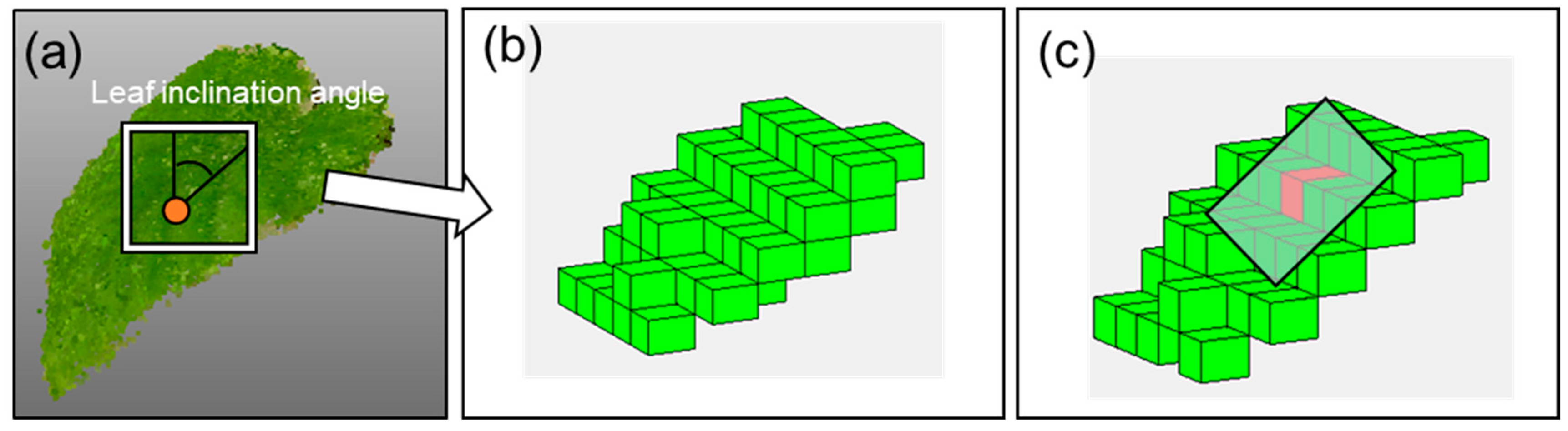
Figure 1.
The leaf inclination angle estimation method. Panel (a) is a three dimensional (3D) leaf image, and it was converted into a voxel-coordinate as shown in the panel (b). The plane fitting was conducted around a voxel and all voxels with an attribute value of 1 among the 342 neighboring voxels (7 × 7 × 7 − 1) around the point (voxel) of interest as shown in the panel (c).

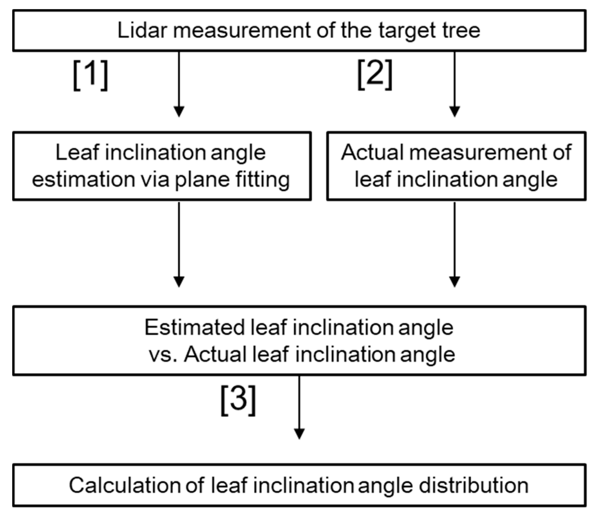
Figure 2.
Flow chart of the experiment.

Figure 3.
Relationship between measured leaf inclination angle and estimated leaf inclination angle (degree).
Figure 3.
Relationship between measured leaf inclination angle and estimated leaf inclination angle (degree).

Figure 4.
Relationship between distance to target leaves from lidar and absolute error of leaf inclination angle estimation.
Figure 4.
Relationship between distance to target leaves from lidar and absolute error of leaf inclination angle estimation.

Figure 5.
Relationship between length of one side of plane for plane fitting and absolute error of leaf inclination angle estimation.
Figure 5.
Relationship between length of one side of plane for plane fitting and absolute error of leaf inclination angle estimation.

Figure 6.
Distribution of leaf inclination angle within a tree (Japanese false oak). Panel (a) shows original image. Panels (b) and (c) show distributions at the top part and lower part, respectively.
Figure 6.
Distribution of leaf inclination angle within a tree (Japanese false oak). Panel (a) shows original image. Panels (b) and (c) show distributions at the top part and lower part, respectively.

Figure 7.
Distribution of leaf inclination angle within a tree (Chinese parasol tree). Panel (a) shows original image. Panels (b) and (c) show distributions at the top part and lower part, respectively.
Figure 7.
Distribution of leaf inclination angle within a tree (Chinese parasol tree). Panel (a) shows original image. Panels (b) and (c) show distributions at the top part and lower part, respectively.

Figure 8.
Distribution of leaf inclination angle within a tree (Japanese Mallotus). Panel (a) shows original image. Panels (b) and (c) show distributions in green part and non-green part, respectively. Criterion of classification is normalized G value of 0.4.
Figure 8.
Distribution of leaf inclination angle within a tree (Japanese Mallotus). Panel (a) shows original image. Panels (b) and (c) show distributions in green part and non-green part, respectively. Criterion of classification is normalized G value of 0.4.

Figure 9.
Distribution of leaf inclination angle within a tree (cherry blossom). Panel (a) shows reconstructed 3D image obtained from lidar. Panels (b) and (c) show distribution map of leaf inclination angle and its distribution, respectively.
Figure 9.
Distribution of leaf inclination angle within a tree (cherry blossom). Panel (a) shows reconstructed 3D image obtained from lidar. Panels (b) and (c) show distribution map of leaf inclination angle and its distribution, respectively.

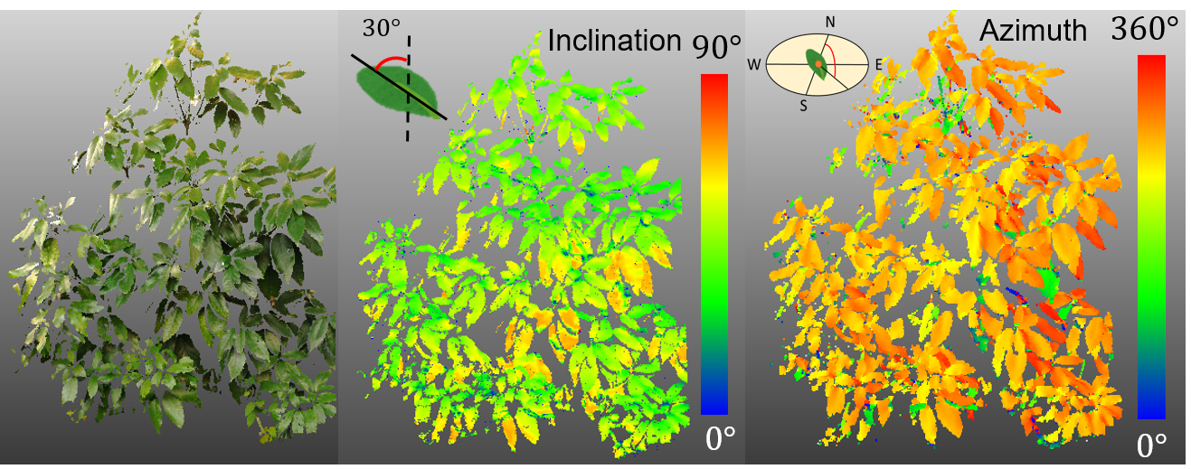
Figure 10.
Distribution of leaf inclination angle and azimuth angle within a tree (Japanese Aucuba). Panel (a) shows reconstructed 3D image obtained from lidar. Panels (b) and (c) show distribution map of leaf inclination angle and azimuth angle, respectively. Panels (d) and (e) show distribution of leaf inclination angle and azimuth angle, respectively.

© 2019 by the authors. Licensee MDPI, Basel, Switzerland. This article is an open access article distributed under the terms and conditions of the Creative Commons Attribution (CC BY) license (http://creativecommons.org/licenses/by/4.0/).
Share and Cite
MDPI and ACS Style
Itakura, K.; Hosoi, F. Estimation of Leaf Inclination Angle in Three-Dimensional Plant Images Obtained from Lidar. Remote Sens. 2019, 11, 344. https://0-doi-org.brum.beds.ac.uk/10.3390/rs11030344
AMA Style
Itakura K, Hosoi F. Estimation of Leaf Inclination Angle in Three-Dimensional Plant Images Obtained from Lidar. Remote Sensing. 2019; 11(3):344. https://0-doi-org.brum.beds.ac.uk/10.3390/rs11030344
Chicago/Turabian StyleItakura, Kenta, and Fumiki Hosoi. 2019. "Estimation of Leaf Inclination Angle in Three-Dimensional Plant Images Obtained from Lidar" Remote Sensing 11, no. 3: 344. https://0-doi-org.brum.beds.ac.uk/10.3390/rs11030344
Note that from the first issue of 2016, this journal uses article numbers instead of page numbers. See further details here.