Statistical Properties of an Unassisted Image Quality Index for SAR Imagery

Abstract

The $\mathcal{M}$ estimator is a recently proposed image-quality index used to evaluate the despeckling operation in SAR (Synthetic Aperture Radar) data. It is used also to rank despeckling filters and to improve their design. As a difference with traditional image-quality estimators, it operates not on the filtered result but on a derived one, i.e., the ratio image. However, a deep statistical analysis of its properties remains open and, with it, the ability to use it as a test statistic. In this work, we focus on obtaining insights into its distribution as well as on exploring other remarkable statistical properties of this unassisted estimator. This study is performed through EDA (Exploratory Data Analysis) and the well-known ANOVA (ANalysis Of VAriance). We test our results on a set of simulated SAR data and provide guides to enrich the $\mathcal{M}$ estimator to extend its capabilities.

1. Introduction

The benefits of SAR (Synthetic Aperture Radar) systems for monitoring planetary surfaces, such as their high-resolution, day and night imaging capability, and being little dependent on the weather, are well-known [1].

It is also well-known that SAR data are corrupted with multiplicative noise (speckle), which can be modelled by a Gamma law [2,3]. Speckle contains valuable information (it can not be regarded to as truly noise) but it hinders proper interpretation of the data and it makes post-processing tasks more complicated, such as image interpretation and classification.

Speckle reduction (despeckling) is an important issue in SAR, and a plethora of excellent despeckling filters have been proposed based on local statistical and adaptive models since the very beginning [4,5,6]. More recently, new approaches include improvement of existing filters [7,8], Nonlocal Means methods [9,10,11], the Curvelet Transform [12,13], the Wavelet Transform [14,15,16], Partial Differential Equations formulation (such as Total Variation and Diffusion-Reaction models) [17,18], or combinations of methods employing Machine Learning techniques [19,20,21]. There are also methods devoted to the multilook case such as [22] which benefits from the sparsity characteristics of speckle to build a non-parametric statistical model for speckle reduction. See an updated tutorial about speckle reduction in [23].

Regarding staircase effect (commonly related to total variation, TV, based methods), a great effort to alleviate this artifact has been done through the either higher-order TV formulations involving complex boundary conditions [24,25], or by splitting techniques for the regularizer [26] or other techniques (in [27], a combination of splitting and penalty technique to solve the model is applied).

Assessing the performances of a despeckling filter is a challenging problem, specially for the state-of-the-art filters: the improvements are likely to be very small, even incremental. Thus, any strategy to confirm that a filter performs better that others should be both efficient and objective. Traditionally, such evaluation relied only on visual inspection of the denoised images [4].

The SAR community has somehow adopted the initial protocol to evaluate despeckling filters proposed by Lee [28] in 1994. It consists of using simulated data: a phantom (truth) image corrupted by speckle noise following a particular distribution, usually the Gamma law. This simulated image is then filtered to obtain the despeckled result. The assessment of the filter operation is done both visually (inspection by an expert) and numerically through a set of measures of quality. Among these, the PSNR (Peak-Signal-to-Noise Ratio), edge preservation (Pratt’s figure of merit, FOM) and image similarity measures (SSIM: structural similarity index) between the original and filtered results are commonly applied. Other first statistical order (mean preservation within homogeneous areas) and second order (variance reduction within homogeneous areas) measures are also applied. After using simulated data, actual cases are evaluated (at least two and with different polarization, number of looks, etc.) and, as no ground-truth is available, the criteria used are mean preservation, variance reduction and visual inspection by an expert. The Lee’s protocol is valid for the one-look and the multilook cases.

Most works in this field propose a new filter, and then compare its performance with existing and closely-related ones. This is usually performed by using simulated data, applying the filters, comparing the results visually and displaying tables or plots with the results of the quantitative assessment [29,30]. A complete review of SAR despeckling assessment can be found in Ref. [1].

Other simulation schemes apart from the one proposed by Lee are also used for the same purpose [11,16], for instance images obtained by means of physical models [17].

Moschetti et al. [31] proposed a MAP (Maximum a Posteriori) despeckling filter. The authors state that

[…] to quantitatively evaluate the results obtained using these new filters, with respect to classical ones, a Monte Carlo extension of Lee’s protocol is proposed. This extension of the protocol shows that its original version leads to inconsistencies that hamper its use as a general procedure for filter assessment.

As a consequence of that, Monte Carlo simulations became a common practical for researchers to better compare filter performance [32,33,34], and also for other SAR/PolSAR (Polarimetric SAR) analyses [35,36].

Recently, a new referenceless image-quality index intended for evaluation of despeckling filters was proposed [37]. This new metric, called $\mathcal{M}$, differently from most of image-quality estimators, obtains valuable information not from the filtered result, but from a derived result: the ratio image.

Evaluation of a filter operation from inspection of the ratio images is inspired from the inspection of residual images after a denoised operation for a image corrupted with additive Gaussian noise. The residual image, R, is obtained as $R=Z-\widehat{X}$, with Z denoting the noisy image and $\widehat{X}$ its filtered version. For an ideal filtering operation, R should contain independent identically distributed Gaussian samples. This kind of complementary evaluation was used in the seminal work by Buades et al. [38] in the introduction of the nonlocal means filters. The use of such alternative approach for the case of multiplicative noise appears in [39] and, from that, many works include this analysis [15,37,40,41] to assess the filter performance.

Assuming the multiplicative model for the speckle within SAR data, the observed image Z is the product of two independent fields: the backscatter X and the speckle Y. The result of any despeckling filter is $\widehat{X}\left(Z\right)$, an estimator of the backscatter X, which only depends on the observed data Z. After the filtering, the ratio image is obtained as $R=Z/\widehat{X}$. If the filter is “perfect”, it contains only speckle, that is, a collection of independent and identically distributed samples from Gamma variates. The new measure is comprised of two terms:

First Order: 

which quantifies deviations from the hypothesis of observing identically distributed deviates from Gamma random variables with unitary mean and same shape parameter, and

Second Order: 

which assesses departures from the independence hypothesis by quantifying the residual geometric content within the ratio image.

Following this idea, Vitale et al. [41] proposed a new second order component: RIS (Ratio Image Structuredness).

Albeit an expressive estimator, the distribution of $\mathcal{M}$ is not known and, therefore, cannot be used as a statistical model [42] for prediction and testing [43,44]. This information would allow to classify filters, to compare the quality of the procedures, to synthesize information and to evaluate fluctuations of the ratio image. Given the difficulty in finding the exact distribution of $\mathcal{M}$, we opt for a nonparametric approach [45].

The organization of this paper is as follows: Section 2 summarizes the $\mathcal{M}$ estimator introduced in [37]. In Section 3 we detail the Monte Carlo experiments on simulated data carried out to obtain the distribution of $\mathcal{M}$, while the mathematical framework is described in Section 4. The results are shown and discussed in Section 5. Final comments and an outline of future research developments are given in Section 6.

2. The $\mathcal{M}$ Estimator

First and for the sake of completeness, we recall the $\mathcal{M}$ estimator and its main properties; see [37] for details about this test statistic.

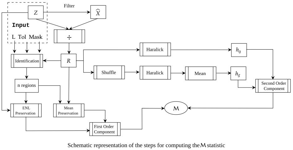
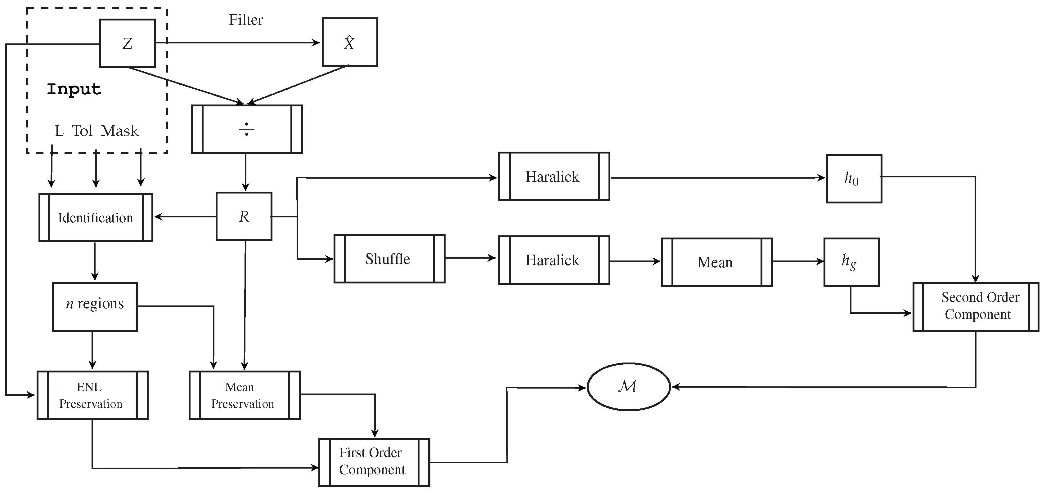
Figure 1 is a schematic representation of the steps leading to the computation of the $\mathcal{M}$ statistic. The required input is identified in the grayed box.

The initial step consists of applying a filter to the original image Z, computing the filtered image $\widehat{X}$ and the ratio image $R=Z/\widehat{X}$.

The test statistic $\mathcal{M}$ is comprised of two terms: one based on first order statistics (mean and number of looks preservation), and one related to second order statistics (independence, or lack of it, of the ratio data).

Computing the first order statistics term requires identifying $n\ge 1$ textureless areas within within the ratio image. Detecting such areas after a reasonable good despeckling operation is a challenging task since most of the data resembles pure noise (speckle). To overcome that, and to avoid any bias from the filtering operation, an automatic detection is performed within the original unfiltered data, and by stipulating a number of looks, a tolerance and a window size.

An automatic search is performed after setting a minimum number of regions to detect, a mask size (i.e., 15) and a tolerance value (i.e., 5%) for the deviation of the estimated ENL (the number of looks of the original SAR data is known). If no area satisfies the setting conditions, they are relaxed by either reducing the size of the mask or by increasing the tolerance related to ENL value. At least ten homogeneous areas were detected in all the experiments carried out in this work. This step is illustrated in the “Identification” box of the schema. Notice that these regions are only used to compute the first-order term of the $\mathcal{M}$ statistic.

Now we calculate the first-order residual as the mean over the n regions identified in the previous step:

$$r_{\widehat{\mathrm{ENL}},\widehat{\mu }}=\frac{1}{2}\sum _{i=1}^n\left(r_{\widehat{\mathrm{ENL}}}\left(i\right)+r_{\widehat{\mu }}\left(i\right)\right),$$

(1)

where, for each textureless area i,

$$r_{\widehat{\mathrm{ENL}}}\left(i\right)=\frac{|{\widehat{\mathrm{ENL}}}_{\mathrm{noisy}}\left(i\right)-{\widehat{\mathrm{ENL}}}_{\mathrm{ratio}}\left(i\right)|}{{\widehat{\mathrm{ENL}}}_{\mathrm{noisy}}\left(i\right)},$$

(2)

is the absolute value of the relative residual due to deviations from the ideal ENL, and

$$r_{\widehat{\mu }}\left(i\right)=|1-{\widehat{\mu }}_{\mathrm{ratio}}\left(i\right)|,$$

(3)

is the absolute value of the relative residual due to deviations from the ideal mean (which is 1). An ideal despeckling operation would yield $r_{\widehat{\mathrm{ENL}},\widehat{\mu }}=0$.

The next step consists of measuring the residual geometric content within the ratio image. We perform this with two quantities derived from a Haralick’s measure of texture, namely:

• $h_{\mathrm{o}}$: the homogeneity of the original ratio image R, and
• $h_g$: the mean homogeneity calculated over 10 randomly shuffled versions of R.

Then, we define $\delta h$ as the absolute value of the relative variation of $h_{\mathrm{o}}$ in percentage as a measure of the departure from the hypothesis that all observations are independent. Note that the larger this variation is, also the greater is the amount of structure remaining on the ratio image. We discretized the observations to eight levels to compute the Haralick measure.

As defined, $\delta h$ provides an objective measure for ranking despeckled results regarding solely the remaining geometrical content within the ratio image. This component increases in the presence of blurred edges, for instance.

By combining the first and second order measures defined above, the proposed estimator provides an estimate of both the remaining structure and of deviations from the marginal statistical properties of the ratio image:

$$\mathcal{M}=r_{\widehat{\mathrm{ENL}},\widehat{\mu }}+\delta h.$$

(4)

The perfect despeckling filter will produce $\mathcal{M}=0$, and the larger $\mathcal{M}$ is, the further apart the filter is from the ideal one.

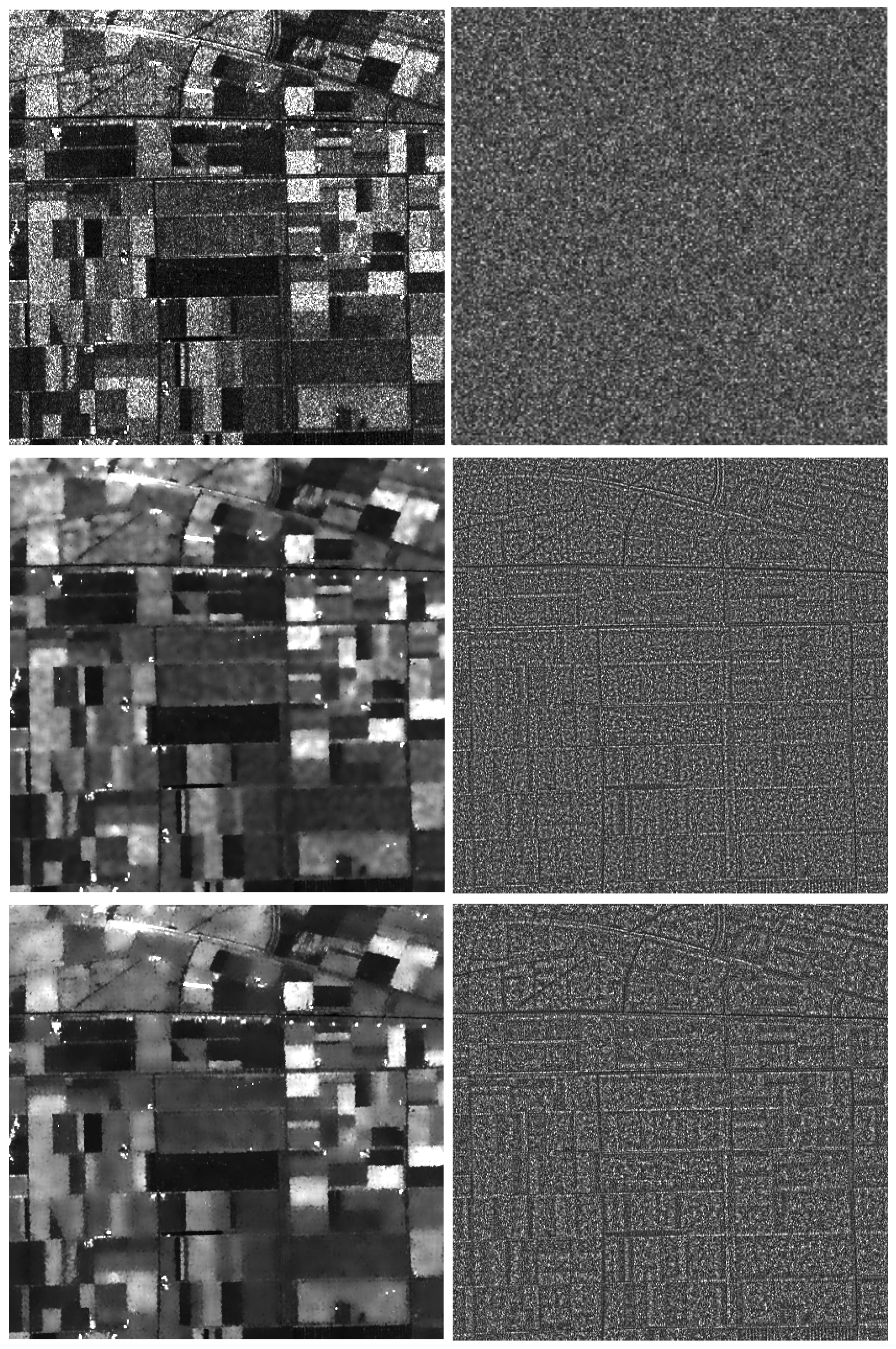
Figure 2 shows observed data, the results of applying two common despeckling filters, the enhanced Lee filter (E-Lee) and FANS (Fast Adaptive Nonlocal SAR) filter for the 4 looks SAR image (Flevoland, Netherlands), and the corresponding ratio images. It can be seen that the result from the FANS filter (third row) is visually superior to the result from the E-Lee filter in terms of edge preservation and also in global appearance. This result is also confirmed visually by inspecting the ratio images: much less geometrical content remains in the ratio image after applying FANS. These subjective results are numerically confirmed by the $\mathcal{M}$ estimator (see

Table 1. $\mathcal{M}$ estimator for the examples shown in Figure 2 and Figure 3.

	${\mathcal{H}}_0$	FANS	E-Lee ($7\times 7$)	E-Lee ($15\times 15$)
$\mathcal{M}$	3.7478	8.1648	20.2215	23.1691

). The $\mathcal{M}$ value for the ${\mathcal{H}}_0$ (the pure speckle data used to compare with) is also shown in this Table.

The $\mathcal{M}$ estimator is also useful to designing despeckling filters. Figure 3 shows two results of applying the E-Lee filter using different mask sizes ($7\times 7$ and $15\times 15$). Notice that the latter filter yields a ratio image with more geometrical content than the solution provided by the design using the $7\times 7$ mask.

The visual inspection of the ratio images suggests that the presence of any remaining structure in the ratio image related to geometric content within the observed image is caused by a non ideal filter. Therefore, edges and small features were been modified (not properly preserved). Regarding bright scatterers, which are of great relevance for despeckling SAR images, note that competitive despeckling filters do not alter significantly their signature of them (the E-Lee filter leaves them without filtering at all) so, no geometrical content remains in the ratio image related to them. All this information is numerically compressed in the $\mathcal{M}$ estimator through the analysis of texture by the $\delta h$ measure.

Although expressive and useful, as seen in the examples above, not knowing the distribution of $\mathcal{M}$ limits its applicability. In particular, we would like to turn it into a test statistic. In the following sections we will tackle this shortcoming.

3. The Distribution of $\mathcal{M}$

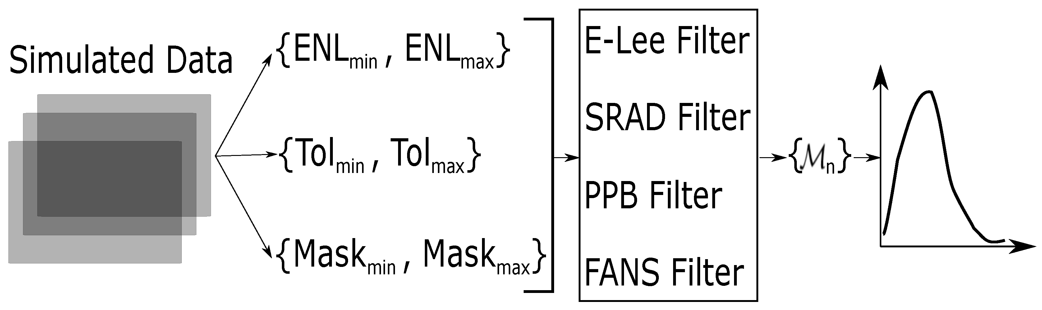
In this section we perform experiments on simulated data to estimate properties of the statistical distribution of $\mathcal{M}$. Figure 4 outlines the methodology we followed.

In order to achieve generality, we employed a parameter space consisting of a set of equivalent number of looks (ranging from ${\mathrm{ENL}}_{min}$ to ${\mathrm{ENL}}_{max}$), Tolerances (from ${\mathrm{Tol}}_{min}$ to ${\mathrm{Tol}}_{max}$) and Mask Sizes (from ${\mathrm{Mask}}_{min}$ to ${\mathrm{Mask}}_{max}$). Then, we applied the same bank of despeckling filters as in [37] to the samples generated. With this we obtain a statistically significant number of samples from $\mathcal{M}$. Then, through the statistical methods described herein below, we infer about the distribution of $\mathcal{M}$.

• Simulated SAR data
  Figure 5 shows the two cases here considered: ramp and step, and an example of their speckled versions in the worst case: one look. The images are are $150\times 150$ pixels.
• Parameters

  -

  ENL: We chose two values for the number of looks: 1 (the worst case) and 4. From the authors’ experience, these two cases are enough for a sound Monte Carlo analysis.

  -

  Tolerance: Tolerance (Tol in Figure 4) refers to the relative deviation from the nominal and estimated values of ENL and the mean, as measured within the observed data in an textureless area. That is, an image region is considered textureless with a tolerance value of, for instance, 5% if its number of looks is, for instance, $L=1$ and the mean value is $\mu =100$, and the measured $\mathrm{ENL}\in [0.95,1.05]$ and the measured $\widehat{\mu }\in [95,105]$. As above, two values for the tolerance have been set: 5% and 10%.

  -

  Window Mask: Window mask (Mask in Figure 4) is the size of the window used to measure ENL and $\mu$. Two values have been set: $15\times 15$ and $25\times 25$.

• Despeckling filters: As mentioned above, the despeckling filters used are the same employed in [37]. They are well-known and with proven efficiency. It is interesting to remark that the four filters are adaptive although conceptually different.

  -

  E-Lee: The Enhanced Lee [7] filter is an improved version of the classical adaptive Lee filter [46]. Its underlying model takes into account an asymmetric distribution for the data.

  -

  SRAD: The Speckle Reducing Anisotropic Diffusion [17] filter belongs to the category of PDE-based (Partial Differential Equations) filters. As a difference with the rest of the filters used in this work, SRAD processes the whole image at once, that is, it is not based on convolution masks.

  -

  PPB: The Probabilistic Patch Based [10] is a nonlocal filter. This filter performs well on images corrupted with both additive and multiplicative noise.

  -

  FANS: The Fast Adaptive Nonlocal SAR [16] filter may be considered state-of-the art among despeckling filters since it provides outstanding results in most cases. FANS employs a set of wavelet transforms in a collaborative fashion with relative low computational cost.

All filters were tuned to the designs recommended by their authors, only with slight modifications (mask size and threshold) for PPB and FANS that yielded improved mean and ENL preservation. This promotes a fair comparison among them.

The next section presents the statistical technique to make inferences about $\mathcal{M}$.

4. Parametric Distribution Analysis

There is a growing tendency of assessing filters in a quantitative, reproducible, and statistically sound manner [31]. This requires going well beyond the use of subjective evaluation. In this sense, the statistical evaluation of quantifiers as the $\mathcal{M}$ may support decisions to manage SAR imagery in an efficient and effective manner.

Analysing $\mathcal{M}$ as a test statistic requires assessing its behavior in two situations: ${\mathcal{H}}_0$, the null hypothesis, and ${\mathcal{H}}_1$, the alternative. The former is that the observations in the ratio image R are a collection of independent and identically distributed deviates from a Gamma law with unitary mean and ENL as shape parameter. The latter, ${\mathcal{H}}_1$, is any deviation from ${\mathcal{H}}_0$. We are interested in the test size and power, related, respectively, to Type I and Type II errors, and to the distribution of $\mathcal{M}$ under ${\mathcal{H}}_0$.

To this end, we perform a Monte Carlo (MC) study, and we consider three situations:

• Experiment 1. Simulation of $\mathcal{M}$ under ${\mathcal{H}}_0$ to evaluate its distribution under the null hypothesis (baseline), i.e., without applying any filter.
• Experiment 2. Simulation of step images, filtering, and then assessing $\mathcal{M}$.
• Experiment 3. Simulation of ramp images, filtering, and then assessing $\mathcal{M}$.

We obtained 100 independent replications in each point of the parameter space. In order to determine a suitable number of replications, we performed an initial analysis in a few selected points of the parameter space with a much larger value.

To evaluate the experiments we use Analysis of Variance—ANOVA [47,48]: a methodology to evaluate combinations of several variables or factors to identify those that have a significant effect on the estimates. The factors under assessment are $\mathrm{ENL}=\{1,4\}$, $\mathrm{Mask}=\{15,25\}$, $\mathrm{Tol}=\{5,10\}$ and $\mathrm{Filter}=\{\mathrm{None},\mathrm{FANS},\mathrm{E}-\mathrm{Lee},\mathrm{PPB},\mathrm{SRAD}\}$. We used a robust linear regression [49] in order to prevent the effect of outliers. Also, we obtained Kernel density estimates of $\mathcal{M}$ using a Gaussian kernel with a fixed smoothing and bandwidth choosing by “rule of thumb” [50].

The robust models used in the analyses were all sequential and with fixed-effects. For each, the variability accounted for was evaluated as adjusted $R^2\times 100$. The models’ fits were compared via ANOVA and robustified F-tests (namely, $F_{\mathrm{R}}$). We performed post-hoc pairwise comparisons [51] with the Tukey’s honestly significant difference test (Tukey’s HSD test), and their p-values were adjusted via false discovery rate ($p_{\mathrm{FDR}}$, see [52]).

5. Experimental Results

5.1. Experiment 1

This experiment provides the core result of this paper: an analysis of the distribution of $\mathcal{M}$ under the (null) hypothesis that the filter is perfect. Under this assumption, the filtered image is exactly the backscatter: $\widehat{X}=X$, so the ratio image is pure speckle $R=Z/\widehat{X}=XY/X=Y$. In this manner, (2) is zero, and the first order component depends only on the mean preservation (3), i.e., $r_{\widehat{\mathrm{ENL}},\widehat{\mu }}=2^{-1}{\sum }_{i=1}^n{r}_{\widehat{\mu }}\left(i\right)$. The second order component is computed at each iteration.

Figure 6 shows the smoothed histograms of the data in all the situations here considered, along with their sample mean (dashed vertical lines).

Table 2. Sample mean ($\overline{\mathcal{M}}$), median ($q_{1/2}\left(\mathcal{M}\right)$), standard deviation ($s_{\mathcal{M}}$), asymmetry (${\gamma }_1\left(\mathcal{M}\right)$) and kurtosis (${\gamma }_2\left(\mathcal{M}\right)$) of the $\mathcal{M}$ statistic in the null hypothesis.

ENL	Tol.	Mask	$\overline{\mathcal{M}}$	${\mathit{q}}_{1/2}\left(\mathcal{M}\right)$	$\mathit{s}\left(\mathcal{M}\right)$	${\mathit{\gamma }}_1\left(\mathcal{M}\right)$	${\mathit{\gamma }}_2\left(\mathcal{M}\right)$
1	5	15	0.0202	0.0201	0.00234	0.2411	2.80
1	10	15	0.0258	0.0258	0.00189	0.0953	3.31
4	5	15	0.0138	0.0138	0.00139	0.0421	2.77
4	10	15	0.0190	0.0189	0.00137	0.3043	3.36
1	5	25	0.0145	0.0145	0.00204	0.4129	3.90
1	10	25	0.0191	0.0191	0.00197	0.2558	3.06
4	5	25	0.0107	0.0105	0.00147	0.3648	2.76
4	10	25	0.0147	0.0145	0.00182	0.1756	2.50

shows the sample mean, standard deviation, asymmetry and kurtosis of $\mathcal{M}$ under the null hypothesis and the eight situations here considered.

We notice the following:

• mean and median are very close, if not identical; this suggests there are no one-sided outliers;
• Tolerance and Mask have less influence on the mean than ENL;
• although systematically positive, the skewness is small;
• kurtosis fluctuates around 3, the value for the Normal distribution, and remains relatively close to it.

In spite of their similarity, the Kolmogorov–Smirnov test rejected the hypothesis that any pair belongs to the same distribution.

For this reason,

Table 3. Critical values of $\mathcal{M}$.

ENL	Tol	Mask	${\mathit{q}}_{950/1000}$	${\mathit{q}}_{990/1000}$	${\mathit{q}}_{999/1000}$
1	5	15	0.0243	0.0250	0.0261
1	10	15	0.0291	0.0299	0.0314
4	5	15	0.0161	0.0163	0.0174
4	10	15	0.0214	0.0226	0.0230
1	5	25	0.0177	0.0204	0.0212
1	10	25	0.0224	0.0239	0.0245
4	5	25	0.0132	0.0142	0.0142
4	10	25	0.0178	0.0186	0.0189

presents the sample critical values at the 5%, 1%, and 1‰ levels for each combination of ENL, Tolerance and Mask. These values allow for testing the hypothesis that a certain filter is ideal at selected significance levels.

As this is the baseline, the kernel density estimators [53,54] of Experiment 1 are shown along the results of other situations.

The normality of the distribution was also checked through the Shapiro–Wilk test [55,56] across parameters. In all cases, the normality is not rejected for usual levels of significance. Usually [57], the thresholds to compare p-values are $0.001$, $0.01$ and $0.05$. Although this would allow us to provide exact rather than sample critical values, using the sample mean and standard deviation provided in Table 2, we opted for the latter in a more conservative approach.

5.2. Experiment 2

Figure 7 shows the kernel density estimates of $\mathcal{M}$ when the filters are applied to the step image. There are noticeable differences in the location the distribution for each combination of parameters when compared to the previous experiment. Also, $\mathcal{M}$ with all filters is more spread than under ${\mathcal{H}}_0$.

Regarding mean values, E-Lee is the closest to ${\mathcal{H}}_0$, closely followed by SRAD, and then by FANS. PPB produces the distribution most shifted to the right, i.e., the one furthest away from the ideal situation.

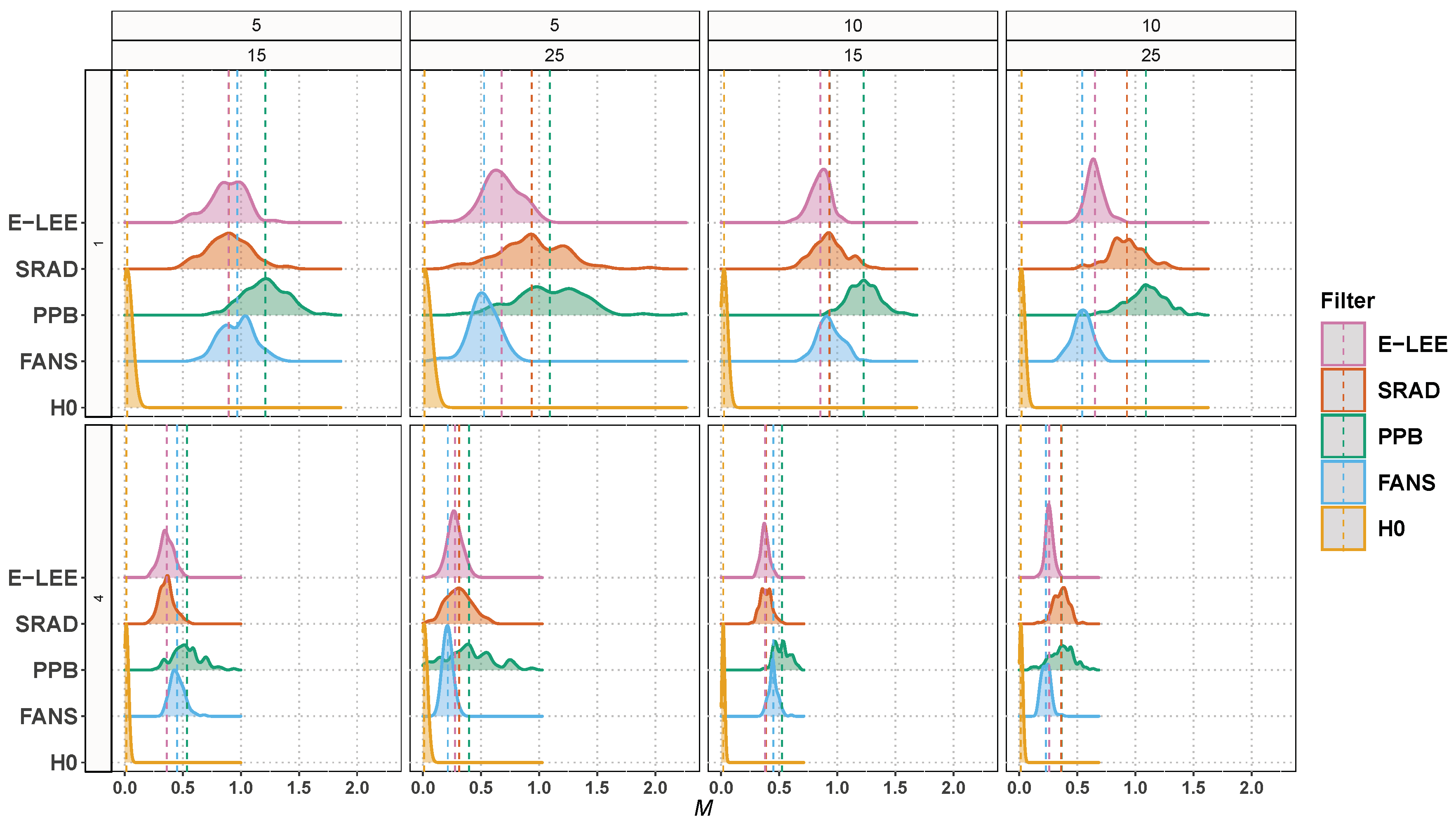
5.3. Experiment 3

Figure 8 shows the kernel density estimates of $\mathcal{M}$ when the filters are applied to the ramp image. We note big differences in the location of the distribution when compared with the baseline. The normality was confirmed in all cases via Shapiro–Wilk.

The distribution of $\mathcal{M}$ with PPB is the worst, as it is the furthest away from $\mathcal{M}$ under ${\mathcal{H}}_0$. A comparison between E-Lee, SRAD and FANS is not conclusive with the single-look ramp, but when the noise is reduced to four looks, SRAD behaves best. This may be due to its global nature, in contrast with the local approach taken by the other filters.

Table 4. Results of the robust linear regression modelling of the data in the four experiments.

Experiment	Model Statistics	${\mathit{F}}_{\mathbf{R}}$	p-Value	VAC (%)
1	ENL model	286.54	$<2{\mathrm{e}}^{-16}$	29.18
	$·\sim ·+\mathrm{Mask}\mathrm{model}$	373.57	$<2{\mathrm{e}}^{-16}$	52.60
	$·\sim ·+\mathrm{Tolerance}\mathrm{model}$	1044.44	$<2{\mathrm{e}}^{-16}$	68.95
2	ENL model	3088.69	$<2{\mathrm{e}}^{-16}$	36.32
	$·\sim ·+\mathrm{Mask}\mathrm{model}$	1133.47	$<2{\mathrm{e}}^{-16}$	40.91
	$·\sim ·+\mathrm{Filter}\mathrm{model}$	433.47	$<2{\mathrm{e}}^{-16}$	61.36
	$·\sim ·+\mathrm{Tolerance}\mathrm{model}$	4.50	0.03	61.42
3	ENL model	2423.97	$<2{\mathrm{e}}^{-16}$	28.77
	$·\sim ·+\mathrm{Mask}\mathrm{model}$	349.30	$<2{\mathrm{e}}^{-16}$	34.28
	$·\sim ·+\mathrm{Filter}\mathrm{model}$	1831.98	$<2{\mathrm{e}}^{-16}$	54.98
	$·\sim ·+\mathrm{Tolerance}\mathrm{model}$	15.67	$<5.29{\mathrm{e}}^{-5}$	55.09

shows the results of the robust linear regression. They suggest that in Experiment 1, $\mathrm{ENL},$ Mask and Tol had an effect on $\mathcal{M}$. All pairwise comparisons were highly significant (${\mathrm{ENL}}_{4\mathrm{vs}.1}=-0.005$, $p_{\mathrm{FDR}}<2{\mathrm{e}}^{-16}$, ${\mathrm{Mask}}_{25\mathrm{vs}.15}=-0.004$, $p_{\mathrm{FDR}}<2{\mathrm{e}}^{-16}$, ${\mathrm{Tol}}_{10\mathrm{vs}.5}=0.004$, $p_{\mathrm{FDR}}<2{\mathrm{e}}^{-16}$).

There were significant effects in the probability distribution of $\mathcal{M}$ in Experiment 2. The mean of all filters is shifted when compared with the baseline. However, we note that, with the exception of PPB, all other filters preserve the shape of the distribution; this suggests stability of distributional family behaviour under ${\mathcal{H}}_0$ across the other parameters. Again, with the exception of Tolerance (${\mathrm{Tol}}_{10\mathrm{vs}.5}=-0.004$, $p_{\mathrm{FDR}}=0.44$), all pairwise comparisons were significant for usual levels of significance:

• ${\mathrm{ENL}}_{4\mathrm{vs}.1}=-0.42$, $p_{\mathrm{FDR}}<2{\mathrm{e}}^{-8}$,
• ${\mathrm{Mask}}_{25\mathrm{vs}.15}=-0.12$, $p_{\mathrm{FDR}}<2{\mathrm{e}}^{-8}$,
• ${\mathrm{Filter}}_{\mathrm{FANS}\mathrm{vs}.{\mathcal{H}}_0}=0.52$, $p_{\mathrm{FDR}}<2{\mathrm{e}}^{-8}$,
• ${\mathrm{Filter}}_{\mathrm{PPB}\mathrm{vs}.{\mathcal{H}}_0}=0.79$, $p_{\mathrm{FDR}}<2{\mathrm{e}}^{-8}$,
• ${\mathrm{Filter}}_{\mathrm{SRAD}\mathrm{vs}.{\mathcal{H}}_0}=0.62$, $p_{\mathrm{FDR}}<2{\mathrm{e}}^{-8}$,
• ${\mathrm{Filter}}_{\mathrm{E}-\mathrm{Lee}\mathrm{vs}.{\mathcal{H}}_0}=0.52$, $p_{\mathrm{FDR}}<2{\mathrm{e}}^{-8}$.

Now, by assessing the ANOVA results in Experiment 3 (see Table 4) using $\mathcal{M}$ as a proxy variable and grouping the data by ENL, Mask and Filter, we obtain statistically significant differences, with the exception of Tolerance which is not significant. The null hypothesis is that the location of $\mathcal{M}$ is the same when the actual effect is a change in dispersion. Clearly, when $\mathrm{ENL}=1$ the E-Lee, SRAD and PPB filters have greater dispersion when compared to FANS. This suggests that the trade-off between bias and variance produced by the FANS filter is smaller, turning the FANS filter more sensitive to detect nuances in the step image, but still it is far from an ideal filter.

We note a paradoxical result by Tukey’s HSD test. PPB and ${\mathcal{H}}_0$ are not significantly different under ${\mathcal{H}}_1$. This is caused by an interaction effect between ENL and Mask, and indicates that PPB is not robust enough to changes in these parameters.

Finally, in Experiment 3, the null hypothesis of the same mean of $\mathcal{M}$ when the parameters are included in the modelling is rejected in all situations (see Table 4).

In this experiment the Tolerance is apparently significant, indicating that the detection of the small nuances is affected by the degree of homogeneity of the image, which was to be expected, i.e., the filters need more specificity to deal with departures from structure detection. However, we observe in the post hoc analysis with the Tukey’s HSD test that Tolerance is not significant ${\mathrm{Tol}}_{10\mathrm{vs}.5}=0.002$, $p_{\mathrm{FDR}}=0.69$). This contradictory result implies that the parameter must be adjusted more carefully. The pairwise comparisons for the other parameters indicate that the differences are statistically significant:

• ${\mathrm{ENL}}_{4\mathrm{vs}.1}=-0.46$, $p_{\mathrm{FDR}}<2.3{\mathrm{e}}^{-8}$,
• ${\mathrm{Mask}}_{25\mathrm{vs}.15}=-0.12$, $p_{\mathrm{FDR}}<2.3{\mathrm{e}}^{-8}$,
• ${\mathrm{Filter}}_{\mathrm{FANS}\mathrm{vs}.{\mathcal{H}}_0}=0.42$, $p_{\mathrm{FDR}}<2.3{\mathrm{e}}^{-8}$,
• ${\mathrm{Filter}}_{\mathrm{PPB}\mathrm{vs}.{\mathcal{H}}_0}=0.87$, $p_{\mathrm{FDR}}<2.3{\mathrm{e}}^{-8}$,
• ${\mathrm{Filter}}_{\mathrm{SRAD}\mathrm{vs}.{\mathcal{H}}_0}=0.53$, $p_{\mathrm{FDR}}<2.3{\mathrm{e}}^{-8}$,
• ${\mathrm{Filter}}_{\mathrm{E}-\mathrm{Lee}}\mathrm{vs}.{\mathcal{H}}_0=0.48$, $p_{\mathrm{FDR}}<2.3{\mathrm{e}}^{-8}$,
• ${\mathrm{Filter}}_{\mathrm{PPB}}\mathrm{vs}.\mathrm{FANS}=0.40$, $p_{\mathrm{FDR}}<2.3{\mathrm{e}}^{-8}$,
• ${\mathrm{Filter}}_{\mathrm{SRAD}}\mathrm{vs}.\mathrm{FANS}=0.06$, $p_{\mathrm{FDR}}<2.3{\mathrm{e}}^{-16}$,
• ${\mathrm{Filter}}_{\mathrm{E}-\mathrm{Lee}}\mathrm{vs}.\mathrm{FANS}=0.01$, $p_{\mathrm{FDR}}=0.63$,
• ${\mathrm{Filter}}_{\mathrm{SRAD}}\mathrm{vs}.\mathrm{PPB}=-0.34$, $p_{\mathrm{FDR}}<2.3{\mathrm{e}}^{-8}$,
• ${\mathrm{Filter}}_{\mathrm{E}-\mathrm{Lee}}\mathrm{vs}.\mathrm{PPB}=-0.39$, $p_{\mathrm{FDR}}<2.3{\mathrm{e}}^{-8}$,
• ${\mathrm{Filter}}_{\mathrm{E}-\mathrm{Lee}}\mathrm{vs}.\mathrm{SRAD}=-0.05$, $p_{\mathrm{FDR}}<1.7{\mathrm{e}}^{-7}$.

Shapiro–Wilks test does not reject the null hypothesis of normality of $\mathcal{M}$ for all combinations of parameters at usual levels of significance.

Simulations and the computation of Haralick’s textural features were performed using Matlab [58]. The data was subsequently analyzed using the R language [59]. Plots and statistical tools were evaluated by available packages in R.

The code and data for reproducing the results here reported are available here https://github.com/Raydonal/Statistical-Behaviour-M-Index.

6. Conclusions

We concluded in this study that the Normal distribution is a suitable model for $\mathcal{M}$ both for the ideal filter (the null hypothesis) and for the alternatives here considered. We observe that, in general, the mean can be assumed as a linear function of ENL and Mask. All filters produced values of $\mathcal{M}$ with approximately Normal distribution shape but with mean values different to those obtained under ${\mathcal{H}}_0$ (Experiment 1).

In this way, we can conduct tests based on normality [60] to evaluate distributional differences between ${\mathcal{H}}_0$ and ${\mathcal{H}}_1$. For example, we can test ${\mu }_{\mathrm{FANS}}-{\mu }_{{\mathcal{H}}_0}=0$ (the difference of means of the residual structure is zero) with a t-test. Here, ${\mu }_{\mathrm{FANS}}$ and ${\mu }_{{\mathcal{H}}_0}$ indicate the expected value of $\mathcal{M}$ using the filter FANS and under ${\mathcal{H}}_0$. In practice, we do not have the mean or variance values. However, we can obtain them using resampling [45] for the filters and by using the simulated values produced as in Section 3 for ${\mathcal{H}}_0$.

References

- Moreira, A.; Prats-Iraola, P.; Younis, M.; Krieger, G.; Hajnsek, I.; Papathanassiou, K.P. A Tutorial on Synthetic Aperture Radar. IEEE Geosci. Remote Sens. Mag. 2013, 1, 6–43. [Google Scholar] [CrossRef]
- Goodman, J.W. Some fundamental properties of speckle. J. Opt. Soc. Am. 1976, 66, 1145–1150. [Google Scholar] [CrossRef]
- Goodman, J.W. Statistical properties of laser speckle patterns. In Laser Speckle and Related Phenomena; Dainty, J.C., Ed.; Springer: Berlin, Germany, 1982; Chapter 2; pp. 9–74. [Google Scholar]
- Lee, J.S. Digital image enhancement and noise filtering by use of local statistics. IEEE Trans. Pattern Anal. Mach. Intell. 1980, 2, 165–168. [Google Scholar] [CrossRef] [PubMed]
- Frost, V.S.; Stiles, J.A.; Shanmugan, K.; Holtzman, J. A model for radar images and its application to adaptive digital filtering of multiplicative noise. IEEE Trans. Pattern Anal. Mach. Intell. 1982, PAMI-4, 157–165. [Google Scholar] [CrossRef]
- Kuan, D.T.; Sawchuk, A.A.; Strand, T.C.; Chavel, P. Adaptive Noise Smoothing Filter for Images with Signal-Dependent Noise. IEEE Trans. Pattern Anal. Mach. Intell. 1985, PAMI-7, 165–177. [Google Scholar] [CrossRef]
- Lee, J.S.; Wen, J.H.; Ainsworth, T.L.; Chen, K.; Chen, A.J. Improved sigma filter for speckle filtering of SAR imagery. IEEE Trans. Geosci. Remote Sens. 2009, 47, 202–213. [Google Scholar]
- Lopes, A.; Nezry, E.; Touzi, R.; Lau, H. Structure detection and statistical adaptive speckle filtering in SAR images. Int. J. Remote Sens. 1993, 14, 1735–1758. [Google Scholar] [CrossRef]
- Liu, Y.; Wang, J.; Xi, C.; Guo, Y.; Peng, Q. A robust and fast non-local means algorithm for image denoising. In Proceedings of the IEEE International Conference on Computer-Aided Design and Computer Graphics, Beijing, China, 15–18 October 2007; p. 30. [Google Scholar]
- Deledalle, C.A.; Denis, F.; Tupin, F. Iterative weighted maximum likelihood denoising with probabilistic patch-based weights. IEEE Trans. Image Process. 2009, 18, 2661–2672. [Google Scholar] [CrossRef] [PubMed]
- Zhong, H.; Li, Y.; Jiao, L. SAR image despeckling using Bayesian nonlocal means filter with sigma preselection. IEEE Geosci. Remote Sens. Lett. 2011, 8, 809–813. [Google Scholar] [CrossRef]
- Sveinsson, J.R. Combined wavelet and curvelet denoising of SAR images using TV segmentation. In Proceedings of the Geoscience and Remote Sensing Symposium (IGARSS’07), Barcelona, Spain, 23–28 July 2007; pp. 503–506. [Google Scholar]
- Schmitt, A.; Wessel, B.; Roth, A. Curvelet approach for SAR image denoising, structure enhancement, and change detection. In Proceedings of the ISPRS, CMRT09, Paris, France, 3–4 September 2009; pp. 151–156. [Google Scholar]
- Argenti, F.; Bianchi, T.; Lapini, A.; Alparone, L. Fast MAP despeckling based on Laplacian-Gaussian modeling wavelet coefficients. IEEE Geosci. Remote Sens. Lett. 2012, 9, 13–17. [Google Scholar] [CrossRef]
- Parrilli, S.; Poderico, M.; Angelino, C.V.; Verdoliva, L. A nonlocal SAR image denoising algorithm based on LLMMSE wavelet shrinkage. IEEE Trans. Geosci. Remote Sens. 2012, 50, 606–616. [Google Scholar] [CrossRef]
- Cozzolino, D.; Parrilli, S.; Scarpa, G.; Poggi, G.; Verdoliva, L. Fast adaptive nonlocal SAR despeckling. IEEE Geosci. Remote Sens. Lett. 2014, 11, 524–528. [Google Scholar] [CrossRef]
- Yu, Y.; Acton, S.T. Speckle reducing anisotropic diffusion. IEEE Trans. Image Process. 2002, 11, 1260–1270. [Google Scholar] [PubMed]
- Zhao, Y.; Liu, J.G.; Zhang, B.; Hong, W.; Wu, Y. Adaptive total variation regularization based SAR image despeckling and despeckling evaluation index. IEEE Trans. Geosci. Remote Sens. 2015, 53, 2765–2774. [Google Scholar] [CrossRef]
- Soccorsi, M.; Gleich, D.; Datcu, M. Huber-Markov model for complex SAR image restoration. IEEE Geosci. Remote Sens. Lett. 2010, 7, 63–67. [Google Scholar] [CrossRef]
- Li, Y.; Gong, H.; Feng, D.; Zhang, Y. An adaptive method of speckle reduction and feature enhancement for SAR images based on curvelet transform and particle swarm optimization. IEEE Trans. Geosci. Remote Sens. 2011, 49, 3105–3116. [Google Scholar] [CrossRef]
- Gomez, L.; Munteanu, C.; Buemi, M.; Jacobo-Berlles, J.; Mejail, M. Supervised constrained optimization of Bayesian nonlocal means filter with sigma preselection for despeckling SAR images. IEEE Trans. Geosci. Remote Sens. 2013, 51, 4563–4575. [Google Scholar] [CrossRef]
- Scarnati, T.; Gelb, A. Variance based joint sparsity reconstruction of synthetic aperture radar data for speckle reduction. Proc. SPIE 2019, 10647R, 1–14. [Google Scholar] [CrossRef]
- Argenti, F.; Lapini, A.; Bianchi, T.; Alparone, L. A Tutorial on Speckle Reduction in Synthetic Aperture Radar Images. IEEE Geosci. Remote Sens. Mag. 2013, 1, 6–35. [Google Scholar] [CrossRef]
- Li, F.; Shen, C.; Fan, J.; Shen, C. Image restoration combining a total variational filter and a fourth-order filter. J. Vis. Commun. Image Represent. 2007, 18, 322–330. [Google Scholar] [CrossRef]
- Liu, G.; Huang, T.; Liu, J. Hig-order TVL1-based images restoration and spatially adapted regularization parameter selection. Comput. Math. Appl. 2014, 67, 2015–2026. [Google Scholar] [CrossRef]
- Xu, J.; Feng, A.; Hao, Y.; Zhang, X.; Han, Y. Image deblurring and denoising by an improved variational model. Int. J. Electron. Commun. 2016, 70, 1128–1133. [Google Scholar] [CrossRef]
- Wang, Y.; Yang, J.; Jin, W.; Zhang, Y. A new alternating minimization algorithm for total variation image reconstruction. SIAM J. Imaging Sci. 2008, 1, 248–272. [Google Scholar] [CrossRef]
- Lee, J.S.; Jurkevich, I.; Dewaele, P.; Wambacq, P.; Oosterlinck, A. Speckle filtering of synthetic aperture radar images: A review. Remote Sens. Rev. 1994, 8, 313–340. [Google Scholar] [CrossRef]
- Gomez, L.; Buemi, M.E.; Jacobo-Berlles, J.; Mejail, M. A new image quality index for objectively evaluating despeckling filtering in SAR images. IEEE J. Sel. Top. Appl. Earth Obs. Remote Sens. 2016, 9, 297–1307. [Google Scholar] [CrossRef]
- Torres, L.; Sant’Anna, S.; Freitas, C.; Frery, A.C. Speckle reduction in polarimetric SAR imagery with stochastic distances and nonlocal means. Pattern Recognit. 2014, 47, 141–157. [Google Scholar] [CrossRef]
- Moschetti, E.; Palacio, M.G.; Picco, M.; Bustos, O.H.; Frery, A.C. On the use of Lee’s protocol for speckle-reducing techniques. Lat. Am. Appl. Res. 2006, 36, 115–121. [Google Scholar]
- Shen, P.; Wang, C.; Gao, H.; Zhu, J. An Adaptive Nonlocal Mean Filter for PolSAR Data with Shape-Adaptive Patches Matching. Sensors 2018, 18, 2215. [Google Scholar] [CrossRef]
- Lang, F.; Yang, J.; Li, D.; Shi, L.; Wei, J. Mean-shift-based speckle filtering of polarimetric SAR data. IEEE Trans. Geosci. Remote Sens. 2014, 52, 4440–4454. [Google Scholar] [CrossRef]
- Xu, B.; Cui, Y.; Zuo, B.; Yang, J.; Song, J. Polarimetric SAR image filtering based on path ordering and simultaneous sparse coding. IEEE Trans. Geosci. Remote Sens. 2016, 54, 4079–4093. [Google Scholar] [CrossRef]
- Fenandez-Michelli, J.I.; Hurtado, M.; Areta, J.A.; Muravchik, C. Unsupervised polarimetric SAR image classification using G0 mixture model. IEEE Geosci. Remote Sens. Lett. 2017, 14, 754–758. [Google Scholar] [CrossRef]
- Xu, J.; Huang, Z.; Yan, L.; Zhou, X.; Zhang, F.; Long, T. SAR Ground Moving Target Indication Based on Relative Residue of DPCA Processing. Sensors 2016, 16, 1676. [Google Scholar] [CrossRef] [PubMed]
- Gomez, L.; Ospina, R.; Frery, A.C. Unassisted quantitative evaluation of despeckling filters. Remote Sens. 2017, 9, 389. [Google Scholar] [CrossRef]
- Buades, A.; Coll, B.; Morel, J.M. A review of image denoising algorithms, with a new one. Multiscale Model. Simul. 2005, 4, 490–530. [Google Scholar] [CrossRef]
- Achim, A.; Kuruoglu, E.; Zerubia, J. SAR image filtering based on the heavy-tailed Rayleigh model. IEEE Trans. Image Process. 2006, 15, 2686–2693. [Google Scholar] [CrossRef]
- Martino, G.D.; Poderico, M.; Poggi, G.; Riccio, D.; Verdoliva, L. Benchmarking framework for SAR despeckling. IEEE Trans. Geosci. Remote Sens. 2014, 52, 1596–1615. [Google Scholar] [CrossRef]
- Vitale, S.; Cozzolino, D.; Scarpa, G.; Verdoliva, L.; Poggi, G. Guided patch-wise nonlocal SAR despeckling. arXiv, 2018; arXiv:1811.11872. [Google Scholar]
- McCullagh, P. What is a statistical model? Ann. Stat. 2002, 30, 1225–1267. [Google Scholar] [CrossRef]
- Thas, O. Comparing Distributions; Springer: Berlin, Germany, 2010. [Google Scholar]
- Cao, R.; Lugosi, G. Goodness-of-fit tests based on the kernel density estimator. Scand. J. Stat. 2005, 32, 599–616. [Google Scholar] [CrossRef]
- Wassermann, L. All of Nonparametric Statistics; Springer: New York, NY, USA, 2006. [Google Scholar]
- Lee, J.S. Speckle Suppression and Analysis for Synthetic Aperture Radar Images. Opt. Eng. 1986, 25, 636–643. [Google Scholar] [CrossRef]
- Montgomery, D.C.; Runger, G.C.; Hubele, N.F. Engineering Statistics; John Wiley & Sons: New York, NY, USA, 2009. [Google Scholar]
- Arias-Castro, E.; Candès, E.J.; Plan, Y. Global testing under sparse alternatives: ANOVA, multiple comparisons and the higher criticism. Ann. Stat. 2011, 39, 2533–2556. [Google Scholar] [CrossRef]
- Yohai, V.J. High breakdown-point and high efficiency robust estimates for regression. Ann. Stat. 1987, 15, 642–656. [Google Scholar] [CrossRef]
- Silverman, B. Density Estimation London; Chapman and Hall: London, UK, 1986. [Google Scholar]
- Rupert, G., Jr. Simultaneous Statistical Inference; Springer Science & Business Media: New York, NY, USA, 2012. [Google Scholar]
- Benjamini, Y.; Hochberg, Y. Controlling the false discovery rate: A practical and powerful approach to multiple testing. J. R. Stat. Soc. Ser. B 1995, 57, 289–300. [Google Scholar] [CrossRef]
- Sheather, S.J.; Jones, M.C. A reliable data-based bandwidth selection method for kernel density estimation. J. R. Stat. Soc. Ser. B 1991, 53, 683–690. [Google Scholar] [CrossRef]
- Fan, J. Local Polynomial Modelling and Its Applications: Monographs on Statistics and Applied Probability 66; Routledge: London, UK, 2018. [Google Scholar]
- Kitchenham, B.; Madeyski, L.; Budgen, D.; Keung, J.; Brereton, P.; Charters, S.; Gibbs, S.; Pohthong, A. Robust statistical methods for empirical software engineering. Empir. Softw. Eng. 2017, 22, 579–630. [Google Scholar] [CrossRef]
- Razali, N.M.; Wah, Y.B. Power comparisons of Shapiro-Wilk, Kolmogorov-Smirnov, Lilliefors and Anderson-Darling tests. J. Stat. Model. Anal. 2011, 2, 21–33. [Google Scholar]
- Dwan, K.; Altman, D.G.; Arnaiz, J.A.; Bloom, J.; Chan, A.W.; Cronin, E.; Decullier, E.; Easterbrook, P.J.; Von Elm, E.; Gamble, C.; et al. Systematic Review of the Empirical Evidence of Study Publication Bias and Outcome Reporting Bias. PLoS ONE 2008, 3, e3081. [Google Scholar] [CrossRef] [PubMed]
- MATLAB. Version 8.3.0.532 (R2014a); The MathWorks Inc.: Natick, MA, USA, 2014. [Google Scholar]
- R Core Team. R: A Language and Environment for Statistical Computing; R Foundation for Statistical Computing: Vienna, Austria, 2018. [Google Scholar]
- Lehmann, E.L.; Romano, J.P. Testing Statistical Hypotheses; Springer Science & Business Media: New York, NY, USA, 2006. [Google Scholar]
Figure 1.
Schematic representation of the steps for computing the statistic.
Figure 2.
Examples of ratio images after filtering the observed data (top) with two despeckling filters. The ideal ratio image is also shown (top right). The filtered image by the enhanced Lee filter ( mask size) is shown in the second row (left) and the ratio image in the same row (right). The filtered image by the FANS filter is shown in the third row (left) and the ratio image in the same row (right).
Figure 3.
Examples of ratio images after filtering the observed data (top) with the same filter but with different designs. The ideal ratio image is also shown (top right). The filtered image by the enhanced Lee filter ( mask size) is shown in the first row (left) and the ratio image in the same row (right). The filtered image by the enhanced Lee filter ( mask size) is shown in the second row (left) and the ratio image in the same row (right).
Figure 4.
Monte Carlo experiments to infer about the distribution of .
Figure 5.
Simulated data used in the Monte Carlo experiments: (top) degraded data and step data (bottom). Bitmap are shown on the left column and simulated samples are shown on the right column.
Figure 6.
Kernel density estimates of the statistic when applied to pure speckle without structure. The vertical dashed lines represent the mean values. is without filtering.
Figure 7.
Kernel density estimates of the statistic when the filters are applied to the step image. The vertical dashed lines are the mean values. H0 is under .
Figure 8.
Kernel density estimates of the statistic when the filters are applied to the ramp image. The vertical dashed lines are the mean values. H0 is under .