Improving the AVHRR Long Term Data Record BRDF Correction

Abstract

The Long Term Data Record (LTDR) project has the goal of developing a quality and consistent surface reflectance product from coarse resolution optical sensors. This paper focuses on the Advanced Very High Resolution Radiometer (AVHRR) part of the record, using the Moderate Resolution Imaging Spectrometer (MODIS) instrument as a reference. When a surface reflectance time series is acquired from satellites with variable observation geometry, the directional variation generates an apparent noise which can be corrected by modeling the bidirectional reflectance distribution function (BRDF). The VJB (Vermote, Justice and Bréon, 2009) method estimates a target’s BRDF shape using 5 years of observation and corrects for directional effects maintaining the high temporal resolution of the measurement using the instantaneous Normalized Difference Vegetation Index (NDVI). The method was originally established on MODIS data but its viability and optimization for AVHRR data have not been fully explored. In this study we analyze different approaches to find the most robust way of applying the VJB correction to AVHRR data, considering that high noise in the red band (B1) caused by atmospheric effect makes the VJB method unstable. Firstly, our results show that for coarse spatial resolution, where the vegetation dynamics of the target don’t change significantly, deriving BRDF parameters from 15+ years of observations reduces the average noise by up to 7% in the Near Infrared (NIR) band and 6% in the NDVI, in comparison to using 3-year windows. Secondly, we find that the VJB method can be modified for AVHRR data to improve the robustness of the correction parameters and decrease the noise by an extra 8% and 9% in the red and NIR bands with respect to using the classical VJB inversion. We do this by using the Stable method, which obtains the volumetric BRDF parameter (V) based on its NDVI dependency, and then obtains the geometric BRDF parameter (R) through the inversion of just one parameter.

1. Introduction

The Advanced Very High-Resolution Radiometer (AVHRR) sensor provides a unique global remote sensing dataset that ranges from the 1980s to the present. Among the different products delivered from this sensor, NASA is currently funding the Long Term Data Record (LTDR) project [1] to develop a quality and consistent Climate Data Record (CDR) of AVHRR data with the use of the Moderate Resolution Imaging Spectrometer (MODIS) instrument as a reference. This data record creates daily global surface reflectance products with a geographic projection at coarse spatial resolution (0.05°). The utility of this long time series has been demonstrated in the literature for a large number of applications such as agriculture [2], burned area mapping [3], Leaf Area Index (LAI) and Fraction of Absorbed Photosynthetically Active Radiation (FAPAR) retrieval [4,5], snow cover estimation [6], global vegetation monitoring [7], and surface albedo estimation products [8,9,10,11].

Long-term consistent data records are becoming crucial to provide improved detection, attribution and prediction of global climate and environmental changes, as well as helping decision makers respond and adapt to climate change and other variability in advance [12,13,14]. The knowledge of surface albedo is of critical importance to monitor land surface processes and plays an important role in energy-budget considerations within climate and weather-prediction models. For this reason, it has been listed as an Essential Climate Variable by the Global Climate Observing System (GCOS) [13,15]. Surface albedo can be derived from satellite data. The most common procedure consists on integrating a BRDF angular model, which can explain the reflectance’s anisotropic behavior on different types of surfaces to obtain the black-sky (direct beam) and white-sky (completely diffuse) narrowband albedo. One can then perform narrow-to-broadband conversions to obtain the respective broadband albedos [16] and obtain the actual (blue-sky) albedo by doing a weighted average, using the fraction of diffuse skylight [17].

For this product to be of highest quality, it is critical that the surface reflectance data record has minimal uncertainties in the calibration, geo-location, spectral correction, cloud masking, atmospheric correction and directional effects correction. Issues regarding calibration, cloud masking and atmospheric correction in the AVHRR data have been accurately corrected, after the year 2000, when MODIS data were used as a reference [2]. However, some issues persist for data before this year (1982–2000), such as aerosol and water vapor correction and calibration [1]. These errors propagate resulting in surface reflectance time series with high noise. This is especially true in the red band, where the atmospheric errors are higher, compared to the Near Infrared (NIR) band. Therefore, the BRDF parameters derived from these time series have high uncertainties and might not provide an accurate correction of the directional effects.

To address this issue, the LTDR product uses MODIS retrieved parameters using the Vermote, Justice and Bréon (VJB) method [18,19] and then applies them to AVHRR data. The VJB method uses a pixel’s time series (typically 5 years) to compute BRDF parameters (V, R) in a daily manner. This is done with the use of the instantaneous Normalized Difference Vegetation Index (NDVI), which quantifies the vegetation by measuring the difference between NIR and red sunlight. These parameters can later be used to correct the database. This method is based on the assumptions that 1) the target reflectance changes during the year but BRDF shape variations are limited and 2) the difference in surface reflectance between successive acquisitions is mostly explained by directional effects.

Assumption 1 holds true while retrieving the correction parameters with short enough periods, or in other words, if the surface doesn’t change significantly over this period. When dealing with AVHRR data, due to the lower number of high-quality observations, a larger number of years is required to make the computation of the BRDF parameters reliable, in which the surface is subject to change. One could argue, however, that because the product is at 0.05° spatial resolution, the stability of the pixel through the years is more likely to be maintained. Assumption 2 holds true for MODIS data because the evolution of the view zenith angle during the year is not gradual, so the difference between successive observations is high, and atmospheric errors are low. This means that the time series have high directional effects, which are higher than the atmospheric correction errors. This is not the case for AVHRR data; the difference of view zenith angle between successive observations is low and atmospheric errors are high, especially for the red band. These facts could justify the use of MODIS parameters to correct AVHRR data, however, these also experience propagated uncertainties caused by the different spectral response of the two sensors or calibration issues of AVHRR.

In this paper we explore different approaches to the AVHRR directional effects correction using the VJB method, to optimize it to AVHRR data. Firstly, we find relationships between BRDF correction parameters using different bands and band combinations derived from MODIS data. With this, we aim to minimize the propagation of atmospheric errors to the correction of directional effects. Secondly, we calculate said parameters using 3 years and the whole time series (15+ years). To test the best method, we compare the noise of the normalized surface reflectance to check which one shows the lowest noise in the time series. Section 2 describes the materials used for the study and the methodology employed. Section 3 presents the results. Section 4 presents a discussion of the results and Section 5 presents the conclusion.

2. Materials and Methods

2.1. Materials

For this study, we downloaded MODIS data from the MOD09 product [20,21] from 2000–2015 and AVHRR from the LTDR product [22]. We divided the data into AVHRR-pre MODIS (1982-2000) and AVHRR (2000–2015). These data contain surface reflectance at Climate Modelling Grid (CMG) spatial resolution (0.05°). We use the red and NIR surface reflectance bands, as well as the view zenith (θv), solar zenith (θs), and relative azimuth (ϕ) angles, selecting pixels of the highest quality. We extracted the data for individual pixels in the 445 Benchmark Land Multisite Analysis and Intercomparison of Products (BELMANIP2) sites. BELMANIP2 sites are an update of BELMANIP1 [23] and were selected due to their representativeness and variability of vegetation types and climatological conditions around the world. Moreover, they were selected so that the sites are homogeneous over a 10 × 10 km² area, so these sites are homogeneous at CMG resolution (0.05° or 5.6 km). We obtained the NDVI from the red and NIR bands from AVHRR-pre, AVHRR and MODIS data. The product includes no spectral adjustment method, which is necessary considering that the time series is composed of data from several different National Oceanic and Atmospheric Administration (NOAA) satellites. Moreover, an accurate intercomparison with MODIS requires that all data be on the same radiometric scale. For this reason, we perform spectral adjustment using methods from Reference [24], selecting NOAA14 as a reference.

2.2. Methods

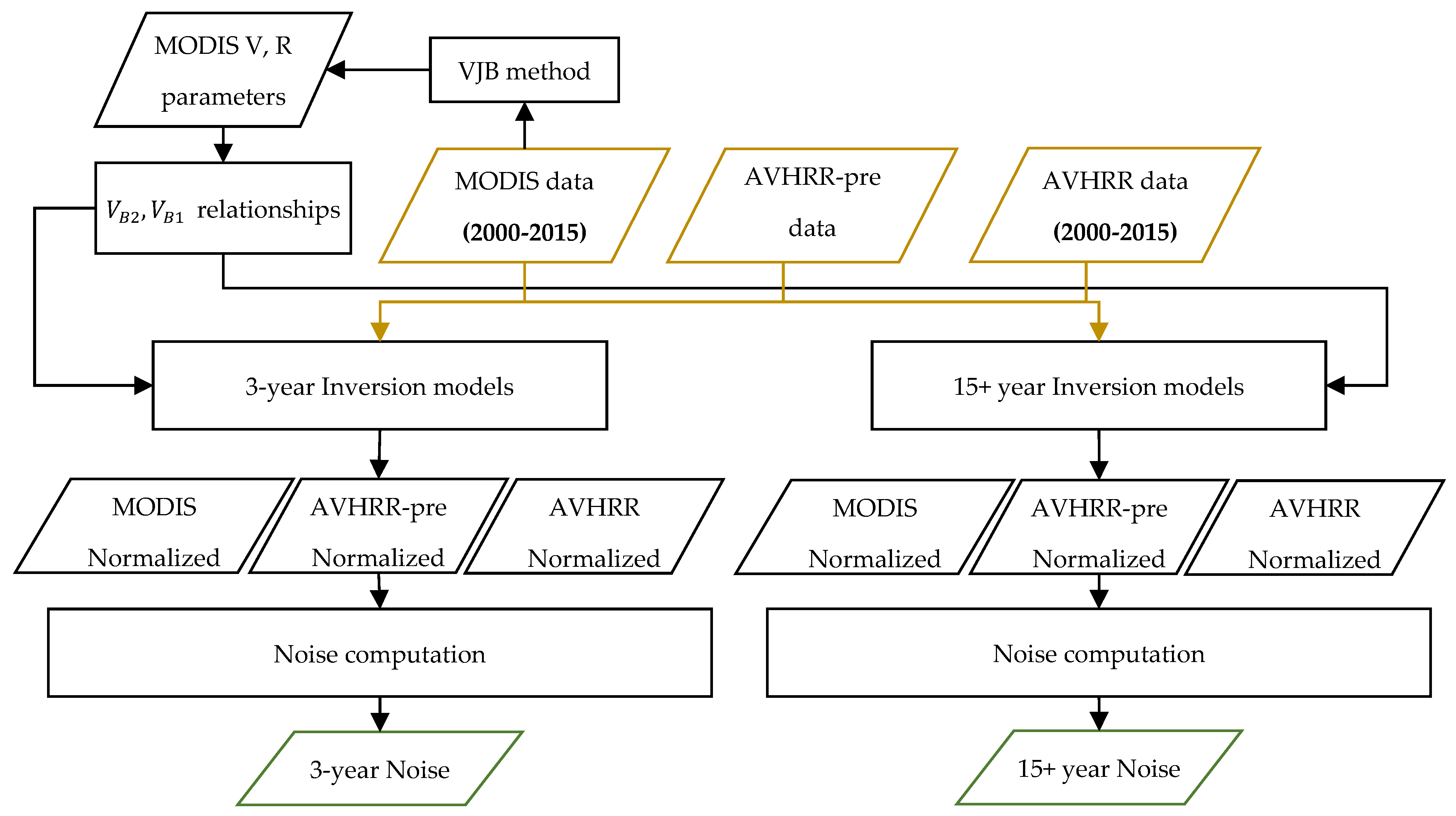
An outline of the methodology is shown in Figure 1 We first use MODIS data to obtain relationships between the BRDF parameters, so we can use them to build different models with AVHRR data. They are then applied to MODIS and AVHRR data, using parameters derived every 3 years, and for the full time series. With these, we derive BRDF correction parameters, which are used to calculate the normalized time series using Equation (9). The normalized NDVI is obtained from the normalized red and NIR reflectances. Finally, given the lack of BRDF field measurements that can be used as a reference to evaluate the best method, we derive the noise of the time series before correction and after the model inversions. This allows us to compare the noise improvement depending on the different BRDF model inversion used, and the number of years employed. The noise is calculated using the statistical difference between the center measurement of three successive triplets and the linear interpolation between the two extremes [18]:

$$Noise\left(y\right)=\sqrt{\frac{{{\displaystyle \sum }}_{i=1}^{n-2}{\left(y_{i+1}-\frac{y_{i+2}-y_i}{da{y}_{i+2}-da{y}_i}\left(da{y}_{i+1}-da{y}_i\right)-y_i\right)}^2}{N-2}}.$$

(1)

2.2.1. VJB Method

The directional effects correction is done using the VJB method, which is based on the Ross Thick Li-Sparse Reciprocal (RTLSR) BRDF model [25,26]. This model expresses the surface reflectance $\rho$ as:

$$\rho \left({\theta }_v,{\theta }_s,\varphi ,t\right)=k_{iso}\left(t\right)\left[1+\mathit{R}{F}_{geo}\left({\theta }_v,{\theta }_s,\varphi \right)+\mathit{V}{F}_{vol}\left({\theta }_v,{\theta }_s,\varphi \right)\right]$$

(2)

where, ($F_{geo},F_{vol}$) are the geometric and volumetric scattering components that provide the basic BRDF shapes for characterizing the heterogeneous scattering of the soil-vegetation system; $(k_{iso}, k_{geo},k_{vol})$ are the weight coefficients of the isotropic, geometric and volumetric kernel functions; V = $k_{vol}/k_{iso}$, R = $k_{geo}/k_{iso}$.

It assumes that the difference between consecutive observations is due principally to directional effects, with small variations of the isotropic weight coefficient k_iso.

$$\frac{\rho \left(t_i\right)}{1+\mathit{V}{F}_{vol}^i+\mathit{R}{F}_{geo}^i}\approx \frac{\rho \left(t_{i+1}\right)}{1+\mathit{V}{F}_{vol}^{i+1}+\mathit{R}{F}_{geo}^{i+1}}.$$

(3)

The values of V and R are the unknowns and can be derived using N observations from a certain pixel by minimizing the merit function:

$$M= {{\displaystyle \sum }}_{i=1}^{N-1}\frac{{\left({\rho }_{i+1}\left[1+V{F}_1^i+R{F}_2^i\right]- {\rho }_i\left[1+V{F}_1^{i+1}+R{F}_2^{i+1}\right]\right)}^2}{da{y}^{i+1}-da{y}^i+1}.$$

(4)

The minimization is done by the classic derivation:

$$\frac{dM}{dV}=\frac{dM}{dR}=0.$$

(5)

This leads to the system of equations:

$$\left(\begin{array}{cc}{\displaystyle {\displaystyle \sum }_{i=1}^{N-1}}{\Delta }^i\rho F_1{\Delta }^i\rho F_1& {\displaystyle {\displaystyle \sum }_{i=1}^{N-1}}{\Delta }^i\rho F_1{\Delta }^i\rho F_2\\ {\displaystyle {\displaystyle \sum }_{i=1}^{N-1}}{\Delta }^i\rho F_1{\Delta }^i\rho F_2& {\displaystyle {\displaystyle \sum }_{i=1}^{N-1}}{\Delta }^i\rho F_2{\Delta }^i\rho F_2\end{array}\right)\otimes \left(\begin{array}{c}V\\ R\end{array}\right)= \left(\begin{array}{c}-{\displaystyle {\displaystyle \sum }_{i=1}^{N-1}}{\Delta }^i\rho {\Delta }^i\rho F_1\\ -{\displaystyle {\displaystyle \sum }_{i=1}^{N-1}}{\Delta }^i\rho {\Delta }^i\rho F_2\end{array}\right)$$

(6)

where:

$${\Delta }^{i}d=da{y}_{i+1}-da{y}_i+1$$

$${\Delta }^i\rho =\left({\rho }_{i+1}-{\rho }_i\right)/\sqrt{{\Delta }^{i}d}$$

$${\Delta }^i\rho F_{1,2}=\left({\rho }_{i+1}{F}_{1,2}^i-{\rho }_{i+1}{F}_{1,2}^{i+1}\right)/\sqrt{{\Delta }^{i}d} .$$

(7)

Through the inversion of Equation (6), we can now obtain a V and R parameter for every pixel. To perform the instantaneous directional correction for every observation, V and R parameters are needed for every date, so the inversion of the V and R parameters is done for five different NDVI populations. A linear regression is performed for V and R as a function of the NDVI (Equation (8)). This retrieves a slope and intercept for every pixel which allow the computation of V and R parameters for a certain date given the surface’s NDVI value.

$$V=V_0+V_1\ast NDVI$$

$$R=R_0+R_1\ast NDVI.$$

(8)

These V and R can now be used to calculate the normalized surface reflectance (${\rho }^N$) at θs = 45°, and nadir observation using Equation (9) [18]:

$${\rho }^N\left(45,0,0\right)=\rho \left({\theta }_s,{\theta }_v,\varphi \right)\ast \frac{1+V{F}_1\left(45,0,0\right)+R{F}_2\left(45,0,0\right)}{1+V{F}_1\left({\theta }_s,{\theta }_v,\varphi \right)+R{F}_2\left({\theta }_s,{\theta }_v,\varphi \right)}$$

(9)

The NDVI can now be obtained using the normalized reflectances:

$$NDV{I}^N=\frac{ {\rho }_{NIR}^N-{\rho }_{red}^N}{ {\rho }_{NIR}^N+{\rho }_{red}^N} .$$

(10)

2.2.2. BRDF Parameters Relationship

To minimize the propagation of the atmospheric errors into the BRDF correction, we analyze the V and R parameters for bands 1 (red) and 2 (NIR). The goal is to find a physical relationship between the BRDF parameters of both bands to avoid using the noisy red AVHRR band. Therefore, we can derive the BRDF parameters of the NIR band and then estimate the red band based on these parameters. To build this physical relationship we use MODIS data since we need data with the least error possible.

To do this, we extract the band 1, band 2 and NDVI time series of one pixel. We then sort them in ascending values of NDVI. We divide these values into five groups, using the 20th, 40th, 60th and 80th percentiles as group edge values. Each of these groups is defined as an NDVI population with its own average. We then extract the V and R values of each one using their band 1, band 2 and NDVI. This means that for every pixel and every band, we obtain 5 different V and R values. When using all the BELMANIP2 sites we obtain a total of 445 × 5 = 2225 points for each band. Finally, we do simple regressions between the obtained parameters for the different bands and with the NDVI itself.

2.2.3. Inversion Period

The idea of this section is to analyze the effect of using a short versus a long period in the computation of the BRDF parameters. For the short period, we use 3 years to make sure the AVHRR time series has enough observations to allow a reliable estimate of parameters. We divided the data from (1982–1999) into three year intervals 1982–1984, 1985–1987, 1988–1990, 1991–1993, 1994–1996, and 1997–1999, and the data from (2000–2015) in 2000–2002, 2003–2005, 2006–2008, 2009–2011, and 2012–2015. For the long period, we use 18 years for AVHRR-pre and 15 years for MODIS and AVHRR. We compute the BRDF parameters using the VJB inversion and the original sensor’s data. In other words, we use MODIS data to calculate MODIS BRDF parameters and AVHRR data to calculate AVHRR BRDF parameters.

2.2.4. Inversion Models

In this section, we compare the different inversion models whose choice is based on different possible hypotheses. The aim is to see which of these are valid for the different data employed. The inversion models used in this paper are the following:

MODIS

We calculate the V and R parameters using the VJB method directly from MODIS data. We hypothesize that calculating BRDF parameters using a time series with small atmospheric and calibration errors provide the best correction. These errors are normally propagated to the correction of directional effects, decreasing the uncertainty of the correction parameters.

AVHRR

Analogous to the MODIS approach, but using AVHRR data. Here we hypothesize that calculating V and R from the sensor we are attempting to correct is more representative than using a different sensor, even if said sensor has less noise in the time series. In other words, we theorize that propagated uncertainties from the atmospheric correction are smaller than data harmonization uncertainties and problems in the original model’s assumption.

Average

Here we make the broad assumption that given the high noise in the AVHRR time series, average V and R parameters which directly depend on the NDVI can be applied. The correction parameters used are derived from Bréon and Vermote [27] and are shown in

Table 1. V(NDVI) and R(NDVI) from [27].

Band 1 (red)	V = NDVI + 0.50	R = 0.20*NDVI + 0.10
Band 2 (NIR)	V = 2.00*NDVI + 0.50	R = −0.05*NDVI + 0.15

.

B1(B2)

Given that the red AVHRR band (B1) is noisy due to the higher errors in the atmospheric correction, we attempt to correct the red band using the parameters from the NIR band. The relationships between them are estimated using MODIS data, which has a robust atmospheric correction and is now a well-established product [28]. We derive the NIR parameters using normal VJB inversion, so one value of V and R for each of the five NDVI populations in each pixel. Then, we apply Equation (10) and continue with the regular VJB method procedure (dependence with NDVI). These relationships are derived in the results section, but are:

$$V_{B1}=0.82\ast V_{B2}+0.11$$

$$R_{B1}=0.91\ast R_{B2}+\mathrm{0.04.}$$

(11)

Stable

In this inversion, we hypothesize that the instability of AVHRR BRDF parameters is due to performing a matrix inversion using two parameters. This provides occasionally very unstable correction parameters when using noisy data. For this reason, we calculate the V_B1 parameter using the NDVI, and the V_B2 parameter from the V_B1. We finally solve R for each band from the second equation of Equation (6). Again, this is done for each of the 5 NDVI populations within every pixel, after which a linear regression with the NDVI is performed.

$$V_{B1}=1.42\ast NDVI+0.63$$

$$V_{B2}=0.83\ast V_{B1}+0.30.$$

(12)

3. Results

3.1. BRDF Parameters Relationship

Figure 2 shows the relationship obtained between V_B1 and V_B2 with the NDVI and between V and R of bands 1 and 2. The r², Root Mean Square Error (RMSE) and linear fit (red line) regression values are shown in the top left of each subplot. The results show that there is a general dependence of the V parameter with the NDVI. This result was expected considering that the V parameter models the volumetric component of the vegetation. A high V value means a denser vegetation, a higher biomass, and effectively a higher NDVI value. However, the high RMSE values both for band 1 and band 2 (0.42,0.45), suggest that this is not a very precise approximation. In the case of the inter-band relationships, the results show that there is a high correlation (r² > 0.8) between the parameters derived from bands 1 and 2. The small RMSE values (0.24,0.04) indicate that this approximation is reliable and could provide a smaller error than that derived by the atmospheric effects propagation from AVHRR or the spectral adjustment and calibration errors from MODIS. The cluster of points that show a 1:1 relation belongs to points with a small NDVI (NDVI < 0.2). Figure 3 shows the relationship between the Band 1 and Band 2 parameters for low NDVI values. It has been shown in previous studies that for low vegetation amount, the R_B1 and R_B2 values are almost identical [25,29]. We also noticed the same behavior for the V parameters, when the NDVI < 0.1. In this study, we also computed the relationship of R with the NDVI, but there was little or no correlation. This is expected considering that the R parameter is associated with the geometric component, and higher NDVI values such as for forests show a similar value to bare ground.

3.2. Inversion Period

Table 2. Average noise (×10⁴) of the Benchmark Land Multisite Analysis and Intercomparison Products (BELMANIP2) sites’ time series obtained before (raw) and after directional effects for the red and Near Infrared bands and the NDVI, using MODIS, the Advanced Very High Resolution Radiometer (AVHRR) pre-MODIS data and AVHRR data from top to bottom. Full and 3-year columns describe the noise after computing the Bidirectional Reflectance Distribution Function (BRDF) parameters using the whole time series, or 3-year intervals, respectively. The percentage under every noise value indicates the improvement with respect to the raw data.

		Red		NIR		NDVI
		Full	3-Year	Full	3-Year	Full	3-Year
MODIS	Raw	201.42	201.42	430.45	430.45	162.21	162.21
	Corrected	48.38 (75.98%)	53.44 (73.47%)	76.23 (82.29%)	107.80 (74.96%)	113.20 (30.22%)	121.19 (25.29%)
AVHRR pre	Raw	212.97	212.97	456.51	456.51	379.83	379.83
	Corrected	130.46 (38.74%)	130.16 (38.88%)	198.10 (56.61%)	230.63 (49.48%)	363.58 (4.28%)	389.08 (−2.43%)
AVHRR	Raw	168.22	168.22	292.62	292.62	317.32	317.32
	Corrected	103.73 (38.34%)	106.58 (36.64%)	144.02 (50.78%)	158.68 (45.77%)	315.33 (0.63%)	319.48 (−0.68%)

shows the average absolute noise (×10⁴) of the BELMANIP sites’ time series obtained when the full dataset and 3-year intervals are used to derive the correction parameters for the red, NIR and NDVI. Inversion using full and 3-year parameters is shown in green and brown font respectively. The percentage under every noise value indicates the improvement with respect to the raw data. For almost every band and dataset, the average noise of the time series using full parameters is lower than using 3-year parameters. In MODIS data, the difference between the full and 3-year parameters is of ~2.5%, 8% and 5% in the red, NIR and NDVI time series noise. This difference is lower for AVHRR-pre (~0%, 7% and 6%) and AVHRR (~2%, 5% and 1%) data.

Effectively, these results show that the effect of the gradual surface change in coarse spatial resolution pixels has little impact on the noise of the time series, as compared with the effect of the number of observations used to compute the parameters. Using a larger number of years retrieves information about the surface which is used in the model to retrieve more accurate parameters and reduce the noise of the normalized time series by a significant amount, especially for the NIR and NDVI.

3.3. Inversion Models

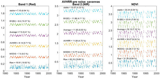
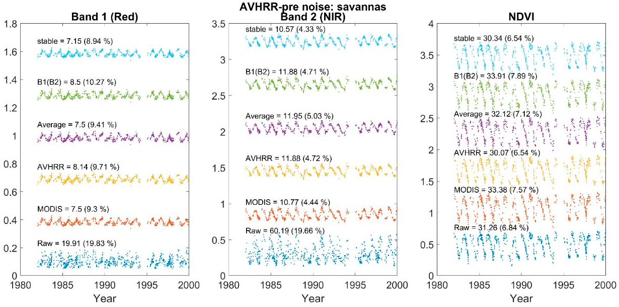
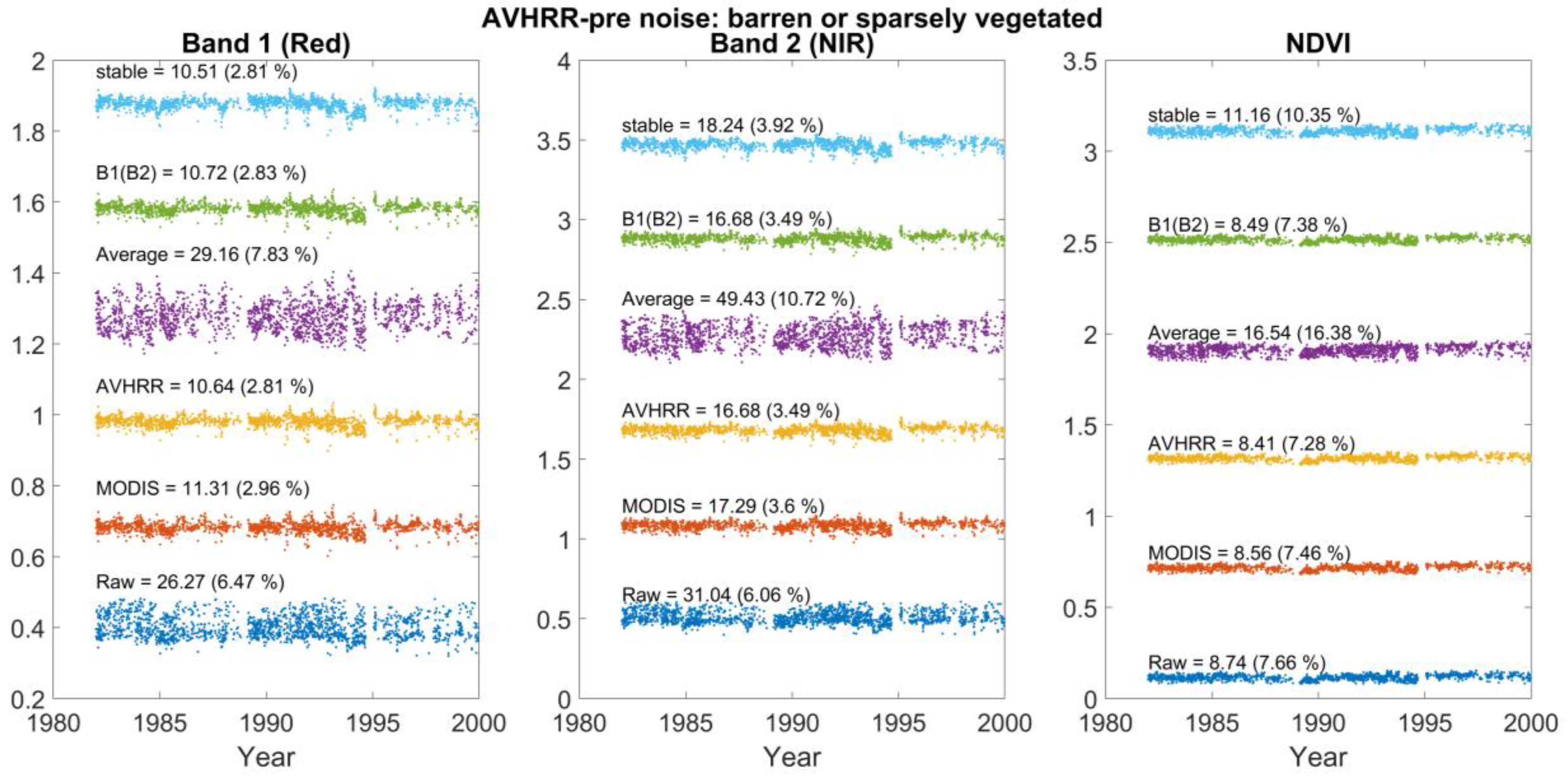
Figure 4 shows the time series of two BELMANIP pixels for different inversion models and their noise value using AVHRR-pre-data. In brackets is shown the relative noise of the time series. For visual purposes, the data is shifted in the y-axis by 0.3 × n in the red and 0.6 × n in the NIR and NDVI for the nth model. The first one is a savanna pixel located in Brazil (−14.72, −41.75). The red and NIR band show a significant improvement in the noise after the directional effects’ correction of ~60% and ~80% respectively, even when using the average method, which is based on the broadest approximation. The result can be appreciated visually, where the seasonal variation of the data can be distinguished after the correction. In the case of the NDVI, however, there is little or no improvement in the noise. When using MODIS parameters, for example, the noise increases. This is due to the intrinsic directional effects’ correction of the NDVI computation [18]. The second pixel is a bare ground pixel located in the Algerian Saharan Desert (28.28, −5.03). In this case, there is also a significant decrease in the red and NIR noise when using the different inversion models, but not in the NDVI. The average method, however, significantly increases the noise, evidencing that the approximation it uses might not be viable for non-vegetated sites. These results also show that the assumption that for low NDVI values, the parameters are the same for both bands is reasonable.

To analyze the performance of every individual model in detail, we plotted the distribution of the noise corrections for every pixel considered in this study. Figure 5 shows these distributions in the form of a boxplot, using the different inversion models and for MODIS, AVHRR-pre and AVHRR data. The top and bottom blue edges of the box represent the 25th and 75th percentiles, respectively, while the middle red line shows the median. Points outside the black bars are considered outliers. The green diamond represents the average of the distribution. These values are shown in

Table 3. Average noise (×10⁴) of the BELMANIP sites’ time series obtained before (raw) and after directional effects using the models described for the red and NIR bands and the NDVI, and using MODIS, AVHRR-pre and AVHRR data from top to bottom. The percentage next to every noise value indicates the improvement with respect to the raw data.

		Red	NIR	NDVI
MODIS	Raw	201.42	430.45	162.21
	MODIS	48.94 (75.70%)	76.23 (82.29%)	113.20 (30.22%)
	Average	90.19 (55.22%)	163.47 (62.02%)	175.16 (−7.98%)
	B1(B2)	53.28 (73.55%)	76.28 (82.28%)	146.00 (10.00%)
	Stable	53.33 (73.52%)	89.74 (79.15%)	136.81 (15.66%)
AVHRR pre	Raw	212.97	456.51	379.83
	MODIS	115.96 (45.55%)	184.07 (59.68%)	396.65 (−4.43%)
	AVHRR-pre	126.98 (40.37%)	198.10 (56.61%)	363.58 (4.28%)
	Average	132.78 (37.65%)	210.16 (53.96%)	394.81 (−3.94%)
	B1(B2)	134.41 (36.89%)	199.32 (56.34%)	397.18 (−4.57%)
	Stable	108.75 (48.93%)	163.30 (64.23%)	368.93 (2.87%)
AVHRR	Raw	168.22	292.62	317.32
	MODIS	103.42 (38.52%)	145.35 (50.33%)	314.67 (0.84%)
	AVHRR	104.08 (38.13%)	144.02 (50.78%)	315.33 (0.63%)
	Average	116.37 (30.82%)	166.03 (43.26%)	329.07 (−3.70%)
	B1(B2)	105.14 (37.50%)	144.74 (50.53%)	315.00 (0.73%)
	Stable	99.28 (40.98%)	140.84 (51.87%)	314.92 (0.76%)

.

Firstly, we can see that the average raw noise of the red and NIR time series is similar for MODIS data (0.020, 0.043) and AVHRR-pre data (0.021, 0.045), but higher than the AVHRR data (0.017, 0.029). This is caused by the large directional errors in MODIS data and the high atmospheric errors in AVHRR-pre-data. Evidence of this can be seen on the NDVI noise. In MODIS, its value is very low (0.016), meaning that the intrinsic directional correction of this index has corrected most of the directional effects. In AVHRR-pre, because the directional effects are not as high, the NDVI correction errors are mostly because of atmospheric uncertainty propagation (0.038).

Secondly, looking at MODIS data (Figure 5, column 1) gives an indication of the quality of the approximations considered by the different models. As is expected, the MODIS inversion provides the best correction (75.7%, 82.3% and 30.2% for the red, NIR and NDVI respectively). Using the Average model, not only is the red and NIR noise improvement lower by ~20%, as compared to the MODIS inversion, but it also has a higher spread of the noise distribution. This is expected considering the broad generalizations of the model. The B1(B2) model shows the second-best performance, only 2% worse than the MODIS inversion, indicating that this a valid approximation that could reduce the computational time while achieving high-quality directional correction. For the NDVI, however, this method shows a significantly smaller improvement (10.0%) than the MODIS model (30.2%). Finally, the Stable method shows to be a valid alternative for the red band, but not for the NIR band. For the NDVI value, it can correct ~5% better than the B1(B2) method.

Analyzing the effects of these models on AVHRR-pre-data (Figure 5, column 2) can now show whether the error provided by their approximations is smaller or higher than the propagated atmospheric error. The MODIS model on AVHRR-pre provides a good correction of the directional effects with ~45.6%, 59.7% in the red and NIR bands, 5% and 3% better than the AVHRR-pre model. This shows that MODIS parameters are preferable to AVHRR-pre derived parameters. The opposite is true for the NDVI. The Average and the B1(B2) model show the worst performances among all of them, with a significant difference with the MODIS model in the red (~8% and 9%) and the NIR (~6% and 3%). This is expected for the Average method but is surprising for the B1(B2) model considering its good performance with MODIS data. It seems like the inversion with two parameters still isn’t good enough, despite having reliable assumptions. In the case of the NDVI, the three of them provide a negative improvement (~4%) given that the noise on the raw data is already low. Finally, the Stable method provides the best improvement in the red and NIR bands, with differences of ~9% and 8% respectively, compared to the AVHRR-pre model. This shows that performing the inversion with one parameter provides higher stability to the parameters and therefore a smaller distribution in the corrected noise values, as can be appreciated by the width of the boxplots in Figure 5. In the NDVI, it provides a positive improvement of 2.87%, but it’s still lower than using the AVHRR-pre-data.

These results are analogous to the AVHRR data (Figure 5, column 3), but with a significantly smaller difference between the methods. The Stable method, for example, only provides a ~3% and 2% improvement difference with the AVHRR model in the red and NIR bands respectively. The average method of AVHRR data improves significantly less than with AVHRR-pre-data. This is because atmospheric errors are not as high in this time series and, therefore, the broad assumptions made by the model provide more uncertainty than the propagated atmospheric perturbations.

4. Discussion

4.1. BRDF Parameters Relationships

The V parameter shows good correspondence with the NDVI, which is expected considering that it models the volumetric component of vegetation. Therefore, it is not surprising that we find a relationship between them. The R parameter can be physically interpreted as the aerodynamic roughness [29]. The relationship between the aerodynamic roughness and the NDVI is not that evident, in fact, we didn’t find any meaningful relationship between the parameters. Given a certain pixel and its geometry, it’s reasonable to think that for higher amounts of vegetation, the aerodynamic roughness is bound to change. In fact, Franch et al., studied the possibility of a quadratic evolution of R with the NDVI within a pixel [30].

Considering that the R parameter is associated with a geometrical component, one would expect it to be independent of the spectral band. Experimental results have shown that this isn’t true and that there is a difference between both values for medium to high NDVI values [25,31,32]. We did find, nevertheless, a good relationship between the R parameter for both bands, which have a slope relatively close to 1 and an intercept close to 0. For low NDVI values, the R parameters are independent of the spectral band. This was also the case for V parameters with NDVI < 0.1, which as far as we are concerned, has never been observed in previous literature.

4.2. Inversion Period

Originally, the VJB method was performed using 5-years of data. The results showed an improvement of ~30% in the NDVI using MODIS data [18], which agree with our results. When including a higher number of years in the inversion, we are increasing the number of observations that are used in the model. This means increasing the range of observation geometries and of possible NDVI values that the pixel can have during the years. However, the accuracy gained by including these observations in the models might be counterbalanced by the change in vegetation characteristics of the target over the years. The larger the amount of years, the more likely it is that this change occurs, and the less likely it is for the assumptions behind the VJB method to hold. Nonetheless, these land cover changes are contemplated to some extent through the NDVI regression implicit in the VJB method. The analysis from this section on the different bands and sensors has shown that this change in vegetation is insignificant compared to the information gained by the increased number of observations. This might only be true, however, so long as the vegetation dynamics or human factors such as deforestation or agricultural practices don’t change the surface value significantly. In these cases, the noise of the time series after BRDF normalization is likely to be high, and a shorter inversion period is recommended that correctly quantifies these land cover changes. When using high spatial resolution, these land cover changes are more discernible than at moderate or high spatial resolution. In this case, a further analysis is required to determine what the adequate inversion period to retrieve the V and R parameters would be.

4.3. Inversion Models

The results of this section show that the conclusions are different for the NDVI correction than for the individual bands. For the red and NIR bands, the Stable model proved to be the best method to use when the data’s time series has too much noise to derive the correction parameters from it. This is true especially for AVHRR-pre, for which the Stable method provided a significant improvement in the noise correction. This is, therefore, the recommended model for the derivation of surface albedo using AVHRR-pre and AVHRR data, provided that the NDVI computation is not required. For MODIS data, the use of the MODIS inversion is still preferable, as assumptions made by the models devised introduce uncertainty. In the case of the NDVI, however, the use of the regular VJB model using parameters derived from the same data is preferred. For users with a large computational burden that look for a compromise between computational time and accuracy, the use of the Average method provides very fast correction parameters at the expense of ~10% noise improvement. If the BRDF correction parameters are already available from MODIS data or another sensor with little atmospheric perturbation at the same spatial resolution, the use of these parameters provides the second best correction after the Stable method with virtually no significant computational time required in comparison.

5. Conclusions

In this paper we explore, different approaches to find the most robust way of applying the VJB correction to AVHRR data. To do this we use AVHRR data from 1982-2015 divided in AVHRR-pre (1982–2000) and AVHRR (2000–2015) and MODIS data (2000–2015) at CMG spatial resolution (0.05°) in 445 BELMANIP2 sites. In the first place, we compare the effect of using 3-years or 15+ years to derive the BRDF parameters. We found that for coarse spatial resolution, where the vegetation characteristics of the target don’t appear to change significantly, it’s preferable to use 15+ years of observation. This result was true both for AVHRR and for MODIS data. The differences were higher for the NIR band, where the average noise was reduced by 7% when using the whole time series from AVHRR-pre-data instead of 3-year parameters.

Secondly, we used MODIS data to retrieve relationships between the BRDF parameters. With the information derived from this sensor, we built different models based on the VJB method, which aim to minimize the propagation of the atmospheric errors present in the AVHRR data to the correction of directional effects. We found that for the red and NIR bands, the Stable method provides a robust correction in terms of reducing both the average noise of the pixels considered and the width of the noise distribution. This is the recommended model for surface albedo retrieval for the VJB method using AVHRR data. For the NDVI, however, we found that the lowest average noise is obtained by correcting MODIS data with MODIS derived parameters and AVHRR data with AVHRR derived parameters. These results are true both for AVHRR-pre which has no aerosol or water vapor correction and for AVHRR, which uses MODIS information for the atmospheric correction.

Further studies should focus on the effect of the spatial resolution on the assumptions made by the VJB method, such as the invariability of a certain site during the composite period of the model. This information is especially useful for the derivation of surface albedo. A surface albedo using AVHRR data from 1982–2018 is of great interest to the scientific community, especially one which relies heavily on observations and on semi-empirical physical models.

References

- Vermote, E.; Claverie, M. Climate Algorithm Theoretical Basis Document (C-ATBD) AVHRR Land Bundle—Surface Reflectance and Normalized Difference Vegetation Index; University of Wisconsin-Madison: Madison, WI, USA, 2013. [Google Scholar]
- Franch, B.; Vermote, E.; Roger, J.-C.; Becker-Reshef, I.; Justice, C.O. A 30+ year AVHRR Land Surface Reflectance Climate 2 Data Record and its application to wheat yield 3 monitoring. Remote Sens. 2016, 9, 296. [Google Scholar] [CrossRef]
- Moreno Ruiz, J.A.; Riaño, D.; Arbelo, M.; French, N.H.F.; Ustin, S.L.; Whiting, M.L. Burned area mapping time series in Canada (1984–1999) from NOAA-AVHRR LTDR: A comparison with other remote sensing products and fire perimeters. Remote Sens. Environ. 2012, 117, 407–414. [Google Scholar] [CrossRef]
- Claverie, M.; Matthews, J.L.; Vermote, E.F.; Justice, C.O. A 30+ Year AVHRR LAI and FAPAR Climate Data Record: Algorithm Description and Validation. Remote Sens. 2016, 8, 263. [Google Scholar] [CrossRef]
- Verger, A.; Baret, F.; Weiss, M.; Lacaze, R.; Makhmara, H.; Vermote, E. Long term consistent global GEOV1 AVHRR biophysical products. In Proceedings of the 1st EARSeL Workshop on Temporal Analysis of Satellite Images, Mykonos, Greece, 23–25 May 2012; Volume 2325, p. 2833. [Google Scholar]
- Wang, S.; Yin, H.; Yang, Q.; Yin, H.; Wang, X.; Peng, Y.; Shen, M. Spatiotemporal patterns of snow cover retrieved from NOAA-AVHRR LTDR: a case study in the Tibetan Plateau, China. Int. J. Dig. Earth 2017, 10, 504–521. [Google Scholar] [CrossRef]
- Julien, Y.; Sobrino, J.A. Monitoring global vegetation with the Yearly Land Cover Dynamics (YLCD) method. In Proceedings of the 2011 6th International Workshop on the Analysis of Multi-Temporal Remote Sensing Images (Multi-Temp), Trento, Italy, 12–14 July 2011; pp. 121–124. [Google Scholar]
- Hu, B.; Lucht, W.; Strahler, A.H.; Barker Schaaf, C.; Smith, M. Surface Albedos and Angle-Corrected NDVI from AVHRR Observations of South America. Remote Sens. Environ. 2000, 71, 119–132. [Google Scholar] [CrossRef]
- Saunders, R.W. The determination of broad band surface albedo from AVHRR visible and near-infrared radiances. Int. J. Remote Sens. 1990, 11, 49–67. [Google Scholar] [CrossRef]
- Strugnell, N.C.; Lucht, W.; Schaaf, C. A global albedo data set derived from AVHRR data for use in climate simulations. Geophys. Res. Lett. 2001, 28, 191–194. [Google Scholar] [CrossRef] [Green Version]
- Trishchenko, A.P.; Luo, Y.; Khlopenkov, K.V.; Wang, S. A Method to Derive the Multispectral Surface Albedo Consistent with MODIS from Historical AVHRR and VGT Satellite Data. J. Appl. Meteor. Climatol. 2008, 47, 1199–1221. [Google Scholar] [CrossRef]
- Bates, J.J.; Privette, J.L.; Kearns, E.J.; Glance, W.; Zhao, X. Sustained Production of Multidecadal Climate Records: Lessons from the NOAA Climate Data Record Program. Bull. Am. Meteorol. Soc. 2015, 97, 1573–1581. [Google Scholar] [CrossRef]
- Hollmann, R.; Merchant, C.J.; Saunders, R.; Downy, C.; Buchwitz, M.; Cazenave, A.; Chuvieco, E.; Defourny, P.; de Leeuw, G.; Forsberg, R.; et al. The ESA Climate Change Initiative: Satellite Data Records for Essential Climate Variables. Bull. Am. Meteorol. Soc. 2013, 94, 1541–1552. [Google Scholar] [CrossRef] [Green Version]
- Schulz, J.; Albert, P.; Behr, H.-D.; Caprion, D.; Deneke, H.; Dewitte, S.; Dürr, B.; Fuchs, P.; Gratzki, A.; Hechler, P.; et al. Operational climate monitoring from space: The EUMETSAT satellite application facility on climate monitoring (CM-SAF). Atmos. Chem. Phys. Discuss. 2008, 8, 8517–8563. [Google Scholar] [CrossRef]
- Bojinski, S.; Verstraete, M.; Peterson, T.C.; Richter, C.; Simmons, A.; Zemp, M. The Concept of Essential Climate Variables in Support of Climate Research, Applications, and Policy. Bull. Am. Meteorol. Soc. 2014, 95, 1431–1443. [Google Scholar] [CrossRef] [Green Version]
- Qu, Y.; Liang, S.; Liu, Q.; He, T.; Liu, S.; Li, X. Mapping Surface Broadband Albedo from Satellite Observations: A Review of Literatures on Algorithms and Products. Remote Sens. 2015, 7, 990–1020. [Google Scholar] [CrossRef] [Green Version]
- Schaaf, C.B.; Gao, F.; Strahler, A.H.; Lucht, W.; Li, X.; Tsang, T.; Strugnell, N.C.; Zhang, X.; Jin, Y.; Muller, J.-P.; et al. First operational BRDF, albedo nadir reflectance products from MODIS. Remote Sens. Environ. 2002, 83, 135–148. [Google Scholar] [CrossRef] [Green Version]
- Vermote, E.; Justice, C.O.; Breon, F.M. Towards a Generalized Approach for Correction of the BRDF Effect in MODIS Directional Reflectances. IEEE Trans. Geosci. Remote Sens. 2009, 47, 898–908. [Google Scholar] [CrossRef]
- Franch, B.; Vermote, E.; Skakun, S.; Roger, J.-C.; Santamaria-Artigas, A.; Villaescusa-Nadal, J.L.; Masek, J. Toward Landsat and Sentinel-2 BRDF Normalization and Albedo Estimation: A Case Study in the Peruvian Amazon Forest. Front. Earth Sci. 2018, 6, 185. [Google Scholar] [CrossRef]
- Vermote, E.F. MOD09A1 MODIS Surface Reflectance 8-Day L3 Global 500m SIN Grid V006; NASA: Washington, DC, USA, 2015.
- Vermote, E.; Vermeulen, A. Atmospheric Correction Algorithm: Spectral Reflectances (MOD09); ATBD: New York, NY, USA, 1999. [Google Scholar]
- LTDR (Land Long Term Data Record) Home. Available online: https://ltdr.modaps.eosdis.nasa.gov/cgi-bin/ltdr/ltdrPage.cgi?fileName=products (accessed on 11 January 2019).
- Baret, F.; Morissette, J.T.; Fernandes, R.A.; Champeaux, J.L.; Myneni, R.B.; Chen, J.; Plummer, S.; Weiss, M.; Bacour, C.; Garrigues, S.; et al. Evaluation of the representativeness of networks of sites for the global validation and intercomparison of land biophysical products: proposition of the CEOS-BELMANIP. IEEE Trans. Geosci. Remote Sens. 2006, 44, 1794–1803. [Google Scholar] [CrossRef]
- Villaescusa-Nadal, J.L.; Franch, B.; Roger, J.; Vermote, E.F.; Skakun, S.; Justice, C. Spectral Adjustment Model’s Analysis and Application to Remote Sensing Data. IEEE J. Sel. Top. Appl. Earth Obs. Remote Sens. 2019, 1–12. [Google Scholar] [CrossRef]
- Roujean, J.-L.; Leroy, M.; Deschamps, P.-Y. A bidirectional reflectance model of the Earth’s surface for the correction of remote sensing data. J. Geophys. Res. 1992, 97, 20455–20468. [Google Scholar] [CrossRef]
- Maignan, F.; Bréon, F.-M.; Lacaze, R. Bidirectional reflectance of Earth targets: evaluation of analytical models using a large set of spaceborne measurements with emphasis on the Hot Spot. Remote Sens. Environ. 2004, 90, 210–220. [Google Scholar] [CrossRef]
- Bréon, F.-M.; Vermote, E. Correction of MODIS surface reflectance time series for BRDF effects. Remote Sens. Environ. 2012, 125, 1–9. [Google Scholar] [CrossRef]
- Vermote, E.F.; El Saleous, N.Z.; Justice, C.O. Atmospheric correction of MODIS data in the visible to middle infrared: First results. Remote Sens. Environ. 2002, 83, 97–111. [Google Scholar] [CrossRef]
- Marticorena; Chazette, P.; Bergametti, G.; Dulac, F.; Legrand, M. Mapping the aerodynamic roughness length of desert surfaces from the POLDER/ADEOS bi-directional reflectance product. Int. J. Remote Sens. 2004, 25, 603–626. [Google Scholar] [CrossRef]
- Franch, B.; Vermote, E.F.; Sobrino, J.A.; Julien, Y. Retrieval of Surface Albedo on a Daily Basis: Application to MODIS Data. IEEE Trans. Geosci. Remote Sens. 2014, 52, 7549–7558. [Google Scholar] [CrossRef]
- Marticorena, B.; Kardous, M.; Bergametti, G.; Callot, Y.; Chazette, P.; Khatteli, H.; Le Hégarat-Mascle, S.; Maillé, M.; Rajot, J.-L.; Vidal-Madjar, D.; et al. Surface and aerodynamic roughness in arid and semiarid areas and their relation to radar backscatter coefficient. J. Geophys. Res. 2006, 111, F03017. [Google Scholar] [CrossRef]
- Franch, B.; Vermote, E.F.; Sobrino, J.A.; Fédèle, E. Analysis of directional effects on atmospheric correction. Remote Sens. Environ. 2013, 128, 276–288. [Google Scholar] [CrossRef]
Figure 1.
Flow diagram of the methodology followed by this study.
Figure 2.
Relationships between VB1, VB2, RB1 and RB2 with each other and the NDVI, derived from the Moderate Resolution Imaging Spectrometer (MODIS).
Figure 3.
Regression between VB1, VB2, RB1 and RB2 for low NDVI values. The red line represents the linear regression fit. The blue line shows the 1:1 line.
Figure 4.
Time series of two BELMANIP pixels (savanna and barren) for different inversion models and their noise value using AVHRR-pre-data. In brackets is shown the relative noise of the time series. For visual purposes, the data is shifted in the y-axis by 0.3n in the red band, and 0.6n in the NIR and NDVI for the nth model.
Figure 5.
Noise distributions for all the bands considered (rows), using the different inversion models and for MODIS, AVHRR-pre and AVHRR data, (columns 1, 2, and 3, respectively). The green diamonds represent the average of the distribution. The top and bottom blue edges of the box represent the 25th and 75th percentiles, respectively, while the middle red line shows the median. Points outside the black bars are considered outliers.