Infrared Small Target Detection Based on Non-Convex Optimization with Lp-Norm Constraint

Abstract

The infrared search and track (IRST) system has been widely used, and the field of infrared small target detection has also received much attention. Based on this background, this paper proposes a novel infrared small target detection method based on non-convex optimization with Lp-norm constraint (NOLC). The NOLC method strengthens the sparse item constraint with Lp-norm while appropriately scaling the constraints on low-rank item, so the NP-hard problem is transformed into a non-convex optimization problem. First, the infrared image is converted into a patch image and is secondly solved by the alternating direction method of multipliers (ADMM). In this paper, an efficient solver is given by improving the convergence strategy. The experiment shows that NOLC can accurately detect the target and greatly suppress the background, and the advantages of the NOLC method in detection efficiency and computational efficiency are verified.

1. Introduction

In recent years, as an indispensable part of infrared search and track (IRST) system, infrared small target detection system is widely used in early warning systems, precision strike weapons and air defense systems [1,2,3]. On the one hand, since the imaging distance is usually several tens of hundreds of kilometers, the signal is attenuated by the atmosphere, and the target energy received by the IRST is weak. For the same reason, the target usually occupies a small area and lacks texture and structural information; on the other hand, the background and noise account for a large proportion, while the background is complex and constantly changing, resulting in a low signal-to-clutter ratio gain (SCR Gain) of the target in the image [4,5,6,7]. Therefore, infrared small target detection methods attract the attention of a large number of researchers [8,9,10].

At present, the mainstream infrared small target detection algorithm can be divided into two major categories: Track before detection (TBD) and detection before track (DBT). Among them, the TBD method jointly processes the information of multiple frames to track the infrared small target, and has higher requirements on computer performance, so the degree of attention is weak. The DBT method is to process the image in a single frame to get the target position, which is usually better in real time and has received more attention. Next, we will introduce the two methods and the research motivation of this article.

1.1. Track before Detection

Track before detection (TBD) methods use spatial and temporal information to estimate the target location by processing multiple adjacent frames. Traditional 3-D matched filtering [11], improved 3-D filtering [12] and Spatiotemporal multiscan adaptive matched filtering [13] are only for static backgrounds. However, the difference between the target and background in the infrared image tends to change rapidly, and the background is also complex and changeable. Therefore, the above methods are not effective.

Braganeto et al. used morphological connected operators to jointly consider target detection and tracking [14]; Dong et al. proposed a novel target detection method [15] by combining the difference of Gaussian (DOG), human visual system (HVS) and clustering methods; Li et al. proposed a biologically inspired multilevel approach for multiple moving target detection [16]; Li et al. proposed a spatio-temporal saliency approach [17]. However, since such methods usually require a large amount of computation and storage, and have high requirements for computer performance, TBD methods are not commonly used in practical applications.

1.2. Detection before Track

Detection before track (DBT) methods usually use the characteristics of small targets to process images on a single frame. The DBT methods can be roughly divided into three categories.

The background suppression based methods. This category of methods is based on the assumption of background consistency of infrared images, and usually adopts filters to suppress background and clutter. The Tophat method [18], Max-Mean and Max-Median method [19], facet model method [20,21] have been proposed and applied to the field of infrared small target detection. However, the assumptions and principles of the background suppression based methods are relatively simple, and the detection effect is not ideal.

The human visual system (HVS) based methods. Borji A [22] pointed out that the contrast between the target and background allows humans to observe small targets. Based on this point, Chen et al. [23] proposed the local contrast method (LCM). It derives the saliency map by sliding the window through each pixel to calculate the local contrast. Han J [24] increased the efficiency of the algorithm by increasing the sliding window step size and proposed improved local contrast method (ILCM). Deng H [25] proposed the weighted local difference measure (WLDM). Wei Y [26] proposed a multiscale patch-based contrast measure (MPCM) after analyzing the characteristics of bright and dark targets. Bai X [27] introduced the concept of derivative entropy into small target detection and proposed a derivative entropy-based contrast measure (DECM). Shi Y [28] proposed a high-boost-based multiscale local contrast measure (HB-MLCM). The prior knowledge of HVS based methods is simple, and usually the computational efficiency is relatively low, so the HVS based methods have been widely used. However, this category of method does not have an ideal facing complex background and noise, leading to low robustness.

The sparse and low-rank matrices recovery based methods. This category considers that the observed image is a linear combination of the target image, the background image, and the noise image, while assuming that the target image is sparse and the background image is low rank. Through the above process, a small target detection problem is transformed into an optimization problem, specifically the robust principal component analysis (RPCA) problem. Gao C [29] used the nuclear norm and the L1-norm as the characteristics of the optimal convex approximation of the rank function and the L0-norm and proposed infrared patch image (IPI) model. He et al. [30] proposed the low-rank representation (LRR) method. Wang C [31] proposed an adaptive target-background separation (T-BS) model. Dai Y [32] applied local steering kernel [33] to the penalty factor and proposed the weighted infrared patch image (WIPI) model. Dai Y [34] improved the way patch images are built, introduced the concept of a tensor [35,36] and proposed a reweighted infrared patch tensor (RIPT) model. Dai Y [37] relaxed the constraint of low-rank, added a non-negative prior, and proposed non-negative infrared patch image (NIPPS) model. Wang X [38] introduced total variation [39,40] to extract sharp edges (TV-PCP) in the infrared image and obtained a purer target image. L Zhang [41] combined the l2,1 norm to describe the background and proposed a novel method based on non-convex rank approximation minimization joint l2,1 norm (NRAM). Since this category of method is assumed to be closer to the real situation, it will perform better than other categories, and with the continuous improvement of the solution algorithm, the convergence speed of such methods is also increasing.

1.3. Motivation

As can be seen from the above, the infrared small target detection methods can be described as a dazzling variety. Among them, the sparse and low-rank matrices recovery-based method has received much attention. However, since such methods usually use the L1-norm as an approximation of the L0-norm, the result may fall into the local minimum rather than the global minimum [42], which affects the constraints of the sparse item; consequently, the detection result is mixed with clutter, and the detection algorithm is poorly robust. Fortunately, there is still much room for improvement in the design of methods.

Previous work has demonstrated that the strategy of using Lp-norm regularization can greatly improve the ability of the algorithm to recover sparse signals compared to the L1-norm [43,44,45,46]. Besides, Lp minimization with 0 < p < 1 recovers sparse signals from fewer linear measurements than does L1 minimization [43]. Another advantage of the Lp-norm is that when a sparse signal can be recovered, it often requires fewer iterations to converge the equation [44]. For RPCA problem, Chen X [47] theoretically established a lower bound of nonzero entries in solution of L2-Lp minimization. Furthermore, recent studies [48,49,50,51] have also given a solution to the RPCA problem of Lp-norm regularization. Although the optimization problem of the Lp-norm is non-convex, it has been studied before, and it has the advantages of being able to obtain a more sparse solution, fewer iterations to converge, and a theoretical basis for the L2-Lp minimization problem. The schatten q-norm can be understood as a sparse constraint on the singular value of the matrix, therefore obeying the above analysis.

Inspired by this, we aim to apply the constraints of the schatten q-norm and Lp-norm to the field of infrared small target detection and propose a novel infrared small target detection method based on non-convex optimization with Lp-norm constraint (NOLC). This method has the advantages of high detection accuracy, anti-noise, and fast convergence. Because of the excellent nature of the Lp-norm, the model is data-driven and can adapt to a variety of complex scenarios.

The main contributions of this article can be summarized as:

(1) Apply schatten q-norm and Lp-norm to the field of infrared small target detection, and propose NOLC method. This method transforms the NP-hard problem into a non-convex optimization problem, and it can restore sparser target images by enhancing constraints on a sparse item.

(2) An optimization solver is given to handle the non-convex optimization problem. This solver combines the ADMM method [52,53,54] to solve the problems. In order to speed up the convergence of this solver, an additional convergence condition is added to it. Similar optimization problems with this model can also use this solver.

(3) Through the specific experimental analysis, this paper gives the influence of different main parameters on the experimental results. Then, the set values of the key parameters are given. The experimental results for real infrared image sequences also verify the feasibility of this method.

The remaining part of this paper is organized as follows: Section 2 shows the principle of the NOLC method and solution of the non-convex optimization problem; Section 3 shows the experimental results, showing the effect of the method by analyzing the real infrared image sequences; The comparison between NOLC and other methods is given in the Section 4, highlighting the difference between this method and others; The conclusion is given in Section 5.

2. Methodology

This section will start with the basic schatten q-norm and Lp-norm, explain the application of these two norms in infrared small target detection, and propose a novel infrared small target detection method based on non-convex optimization with Lp-norm constraint (NOLC). Finally, a concrete solution method combining ADMM of this optimization is given.

2.1. Schatten q-norm and Lp-norm

Assume that matrix A has singular value decomposition $A=U\ast S\ast V^T$, where S denotes the singular value diagonal matrix. As we all know, the definition of the two norms of A is as Equations (1) and (2), where ${\Vert A\Vert }_{sq}$ represents schatten q-norm and ${\Vert A\Vert }_p$ represents Lp-norm.

$${\Vert A\Vert }_{sq}={\left({\displaystyle \sum _{i=1}^{\min \{m,n\}}{\sigma }_i^q}\right)}^{1/q},0<q<\infty$$

(1)

$${\Vert A\Vert }_p={\left({\displaystyle \sum _{i=1}^m{\displaystyle \sum _{j=1}^n{\left|a_{ij}\right|}^p}}\right)}^{1/p},0<p<\infty$$

(2)

where ${\sigma }_i$ represents the ith singular value of matrix A, or can be expressed as the ith diagonal component of S; $a_{ij}$ represents the pixel value of the ith row and the jth column of the matrix A. Since the matrix singular value is non-negative, the schatten q-norm of matrix A can be regarded as the Lp-norm of S. Therefore, we can understand the Schatten q-norm as a sparse constraint on singular values and it also obeys the following analysis of the Lp-norm.

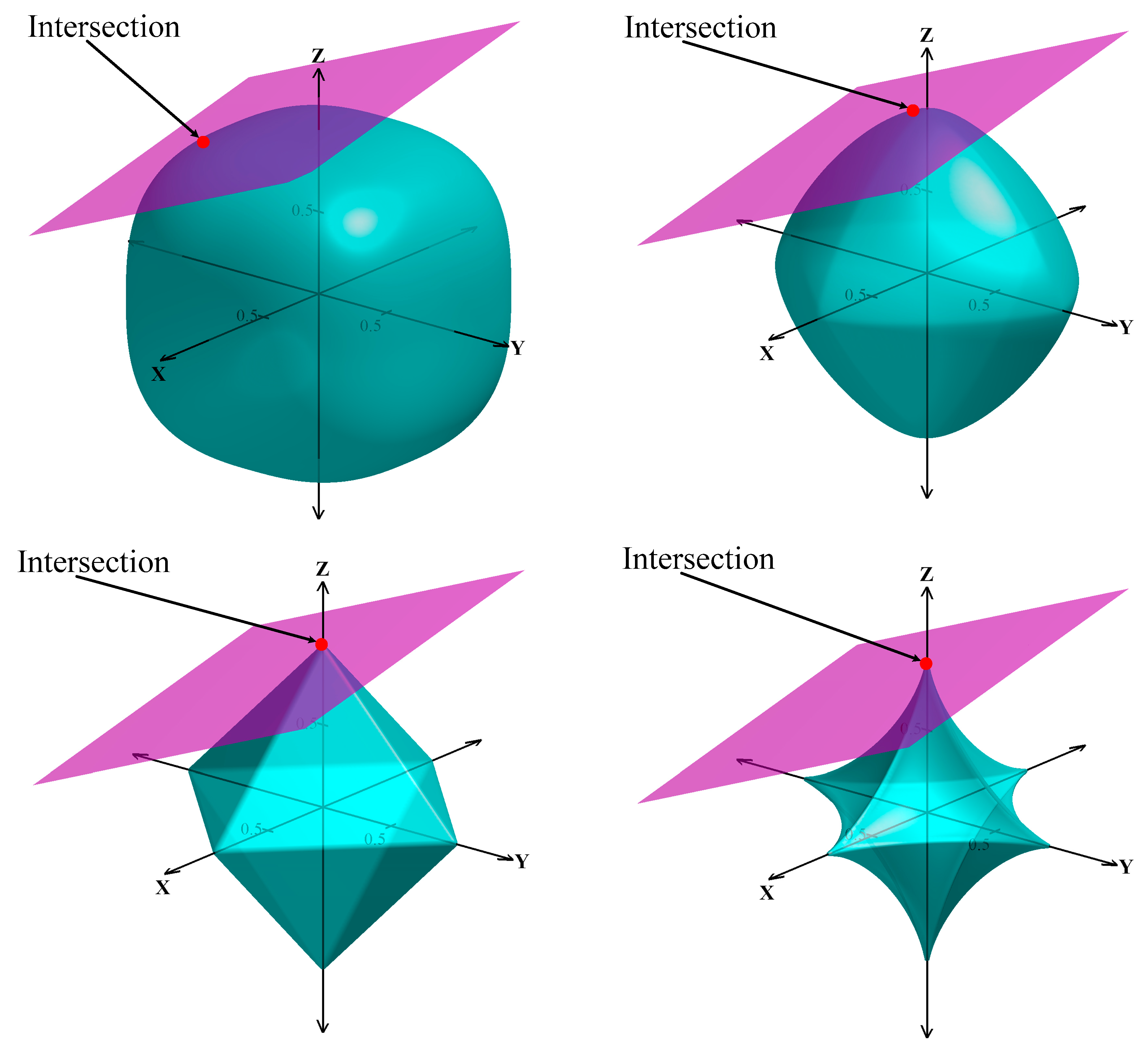
For the optimization problem in Equation (3), geometrically, the constraint is a hyperplane and the Lp-norm is a ball blown from the origin point. As shown in Figure 1, when the blown ball is in contact with the hyperplane for the first time, the intersection is the optimal solution of problem (3).

$$\underset{X}{\min }{\Vert X\Vert }_p^{p}s.t.AX=b$$

(3)

Figure 1 shows the geometry of p when taking different values in 3D space. It can be seen that when p is greater than 1, the obtained optimal solution is not sparse, and when p is less than or equal to 1, the intersection point is on the coordinate axis, and two of the three elements are 0, so the optimal solution is sparse. Therefore, it can be geometrically stated that a sparse solution can be obtained when p is less than or equal to 1.

Broadly speaking, the values of p in the Equation (2) can range from 0 to positive infinity. But, in order to obtain the sparse solution, only the case where p is less than or equal to 1 is considered. In the special case where q and p equal to 0, the two norms can be expressed as Equations (4) and (5), where Equation (4) is a constraint on low rank and Equation (5) is a constraint on sparseness.

$${\Vert A\Vert }_{s0}=\#(i)with{\sigma }_i\ne 0=rank(A)$$

(4)

$${\Vert A\Vert }_0=\#(i)with{a}_i\ne 0$$

(5)

However, these two functions above are non-convex and very difficult to solve, so they need to be approximated. Another special case is when q and p equal to 1, shown in Equations (6) and (7). These two norms are used in the reference [29] to approximate Equations (4) and (5) and constrain low rank and sparseness. Since Equations (6) and (7) are convex function, sub-problems with these two norm constraints can be easily solved.

$${\Vert A\Vert }_{s1}={\displaystyle \sum _{i=1}^{\min \{m,n\}}{\sigma }_i}={\Vert A\Vert }_{\ast }$$

(6)

$${\Vert A\Vert }_1={\displaystyle \sum _{i=1}^m{\displaystyle \sum _{j=1}^n\left|a_{ij}\right|}}$$

(7)

From the above analysis, the IPI model in reference [29] is a special case of the schatten q-norm and Lp-norm in this paper. It is worth mentioning that the strategy of using Lp-norm regularization can greatly improve the ability of the algorithm to recover sparse signals compared to the L1-norm [43,44,45,46]. Another advantage of the Lp-norm is that when a sparse signal can be recovered, it often requires fewer iterations to converge the equation. Based on this knowledge, we begin to introduce the model proposed in this paper.

2.2. The Proposed Method

In reference [10], when the noise can be approximated as additive, and the infrared small target image can be seen as a linear combination of target image, background image, and noise image. This assumption is also widely used in future models [30,31,32,33,34]. This model can be represented by the following equation.

$$f_D=f_B+f_T+f_N$$

(8)

where $f_D$ denotes the infrared image; $f_B$, $f_T$ and $f_N$ represent the target image background image and noise image, respectively. Among them, because the target occupies a small area, it can be considered as a sparse matrix. The background contains many repetitive elements, so it can be considered as low rank matrix. The target image can be recovered by solving the model.

Then, by transforming the original image with the sliding window into patch image, the sparsity of the target and the low rank of the background are enhanced. The model is transformed into Equation (9):

$$D=B+T+N$$

(9)

where $D$, $B$, $T$ and $N$ denotes the patch images. Subsequently, we apply constraints on $B$ and $T$ using schatten q-norm and Lp-norm, respectively, and propose a method based on non-convex optimization with schatten q-norm and Lp-norm constraint (NOSLC). The objective function is expressed as follows.

$$\underset{B,T}{\min }{\Vert B\Vert }_{sq}^q+\lambda {\Vert T\Vert }_p^{p}s.t.{\Vert D-B-T\Vert }_F\le \delta$$

(10)

where $\lambda$ is the penalty factor and $\delta$ denotes the noise level in the image; ${\Vert •\Vert }_F$ denotes the Frobenius norm which is a special case of Lp-norm when p equals to 2.

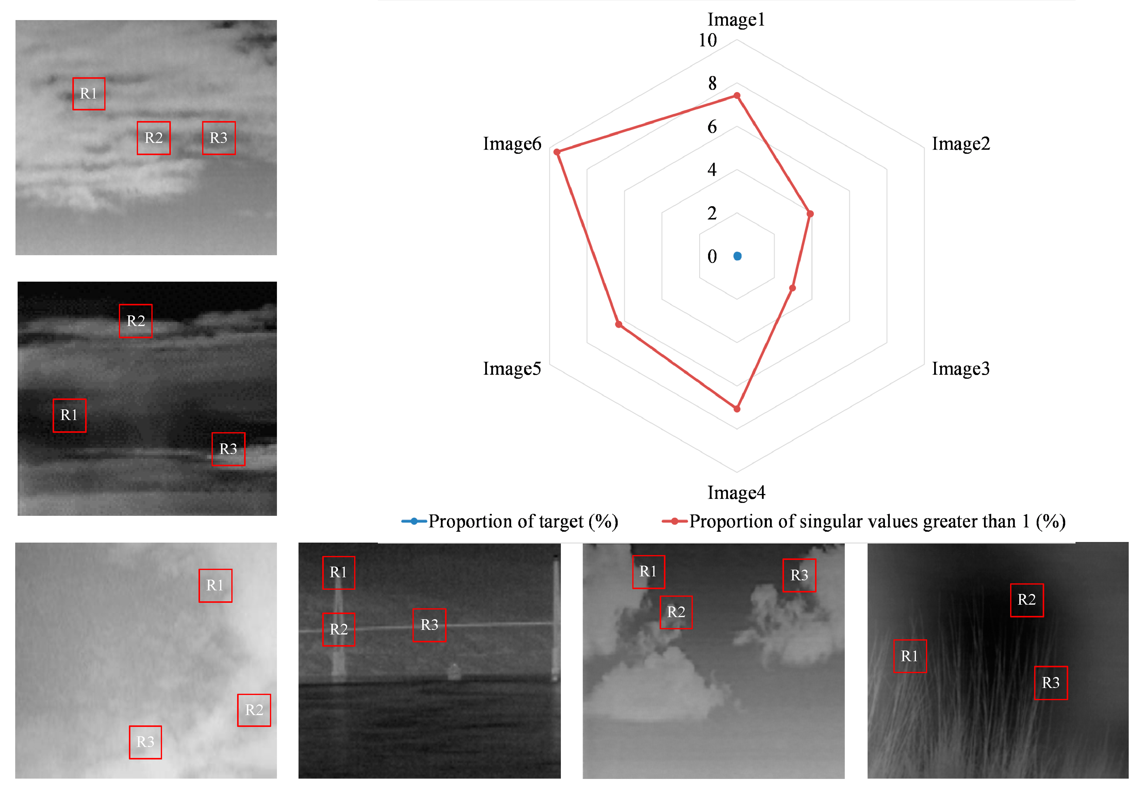
As we mentioned earlier, the smaller the q and p values, the stronger the constraint on low rank and sparsity. However, we analyzed the real infrared image and found that the low rank property of the background patch image is not very strict compared to the sparsity of the target patch image.

Figure 2 shows the proportion of singular values greater than one and the proportion of target pixels for different infrared images. In the figure, six infrared images are analyzed, wherein the marked regions R1 to R3 are patch images with relatively large background changes, and are also regions that make the low rank property of background image less stringent. In the radar chart, the red dots indicate the proportion of singular values greater than 1, and the blue dots indicate the proportion of targets. It is obvious that the blue dots are squeezed together because their value is much smaller than that of the red dots. This image also shows that the sparsity of the target should be stricter than the low rank property of the background.

Based on the above description, we know that it is unscientific to impose strong constraints on both the low rank property and sparsity, so we relax the constraint on the low rank property and let q equal to 1. Then, we propose a method based on non-convex optimization with Lp-norm constraint (NOLC). The objective function is shown in Equation (11).

$$\underset{B,T}{\min }{\Vert B\Vert }_{\ast }+\lambda {\Vert T\Vert }_p^{p}s.t.{\Vert D-B-T\Vert }_F\le \delta$$

(11)

where ${\Vert B\Vert }_{\ast }$ denotes the nuclear norm of matrix $B$ which is the special case of the schatten q-norm when q equals to 1. We have scaled down the constraints on low-rank property, so the model is not as sensitive as NOSLC to structural clutter in the background image which is inevitable. We qualitatively consider the two models presented above, and the NOLC method will achieve better results.

2.3. Solution of NOLC model

We obtained the physical model and objective function that we need to solve from the previous section. In this section we will give the solution to the NOLC model. Combined with the ADMM method, the Lagrange function of the objective function (11) is shown by Equation (12).

$$L\left(B,T,Y\right)={\Vert B\Vert }_{\ast }+\lambda {\Vert T\Vert }_p^p+\langle Y,D-B-T\rangle +\frac{\rho }{2}{\Vert D-B-T\Vert }_F^2$$

(12)

where $\langle •,•\rangle$ represents the inner product of two matrices, $\rho$ is a penalty factor and $Y$ is Lagrange multiplier matrix. Now we need to use an iterative method to minimize the Lagrange function. In this process, two sub-problems are solved. Next, we explain their solution method separately.

(a) The First Sub-Problem

The function is as follows:

$$\begin{array}{cc}\hfill B^{k+1}& =\arg \underset{B}{\min }L\left(B,T^k,Y^k\right)\hfill \\ & =\arg \underset{B}{\min }{\Vert B\Vert }_{\ast }+\frac{\rho }{2}{\Vert B-\left(D+{\rho }^{-1}{Y}^k-T^k\right)\Vert }_F^2\hfill \end{array}$$

(13)

The above formula is a convex optimization problem and can be solved by the singular value shrinkage operator [54].

$$B^{k+1}=Q\ast S_{{\rho }^{-1}}[diag(\sum )]\ast R^T$$

(14)

where $Q$, $\sum$, $R$ represents the singular value decomposition of matrix $D^k+{\rho }^{-1}{Y}^k-T^k$, that is to say $D^k+{\rho }^{-1}{Y}^k-T^k=Q\ast \sum \ast R^T$; $diag(\sum )$ denotes the diagonal elements of matrix $\sum$; $S_{{\rho }^{-1}}[•]$ is the soft thresholding operator; its definition is given in the following formula.

$$S_{\epsilon }[x]=\{\begin{array}{ll}x-\epsilon \hfill & ifx>\epsilon \hfill \\ x+\epsilon \hfill & ifx<-\epsilon \hfill \\ 0\hfill & others\hfill \end{array}$$

(15)

(b) The Second Sub-Problem

For the second sub-problem, a non-convex optimization problem is involved.

$$\begin{array}{cc}\hfill T^{k+1}& =\arg \underset{T}{\min }L\left(B^{k+1},T,Y^k\right)\hfill \\ & =\arg \underset{T}{\min }\lambda {\Vert T\Vert }_p^p+\frac{\rho }{2}{\Vert T-\left(D+{\rho }^{-1}{Y}^k-B^{k+1}\right)\Vert }_F^2\hfill \end{array}$$

(16)

Since the elements in the matrix are linearly independent, this problem can be refined to each pixel to solve [50]. For each pixel, the optimization goal is:

$$x^{\ast }=\underset{x}{\min }\frac{1}{2}{\left(x-a\right)}^2+\lambda {\left|x\right|}^p$$

(17)

Let the optimization function of each pixel be $g\left(x\right)$.

$$g\left(x\right)=\frac{1}{2}{\left(x-a\right)}^2+\lambda {\left|x\right|}^p$$

(18)

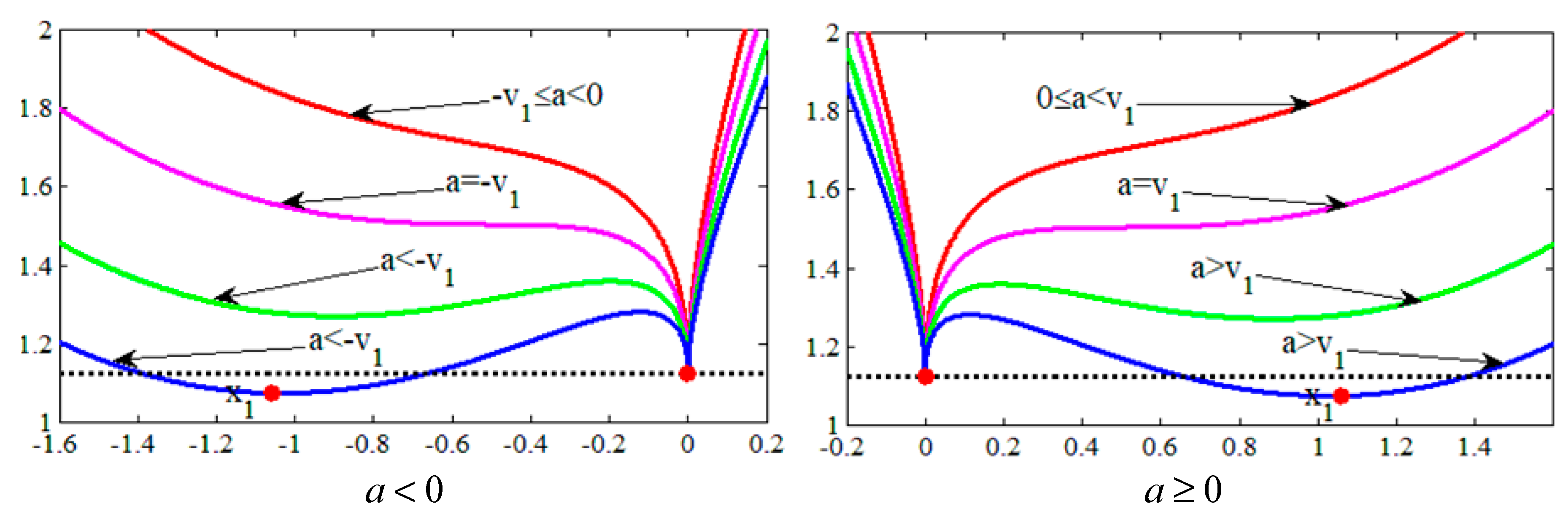
In problem (17), we want to get the corresponding $x$ value when $g\left(x\right)$ is the smallest. The curve of this function is shown in Figure 3. Obviously $g\left(x\right)$ is not a convex function, but the minimum point of $g\left(x\right)$ is easy to find.

By analyzing the first second and third derivative of $g\left(x\right)$, we can get the minimum point of $g\left(x\right)$, either 0 or $x_1$. We set two parameters $v={\left(\lambda p\left(1-p\right)\right)}^{\frac{1}{2-p}}$ and $v_1=v+\lambda p{\left|v\right|}^{p-1}$. The solution to problem (17) is:

$$x^{\ast }=\{\begin{array}{cc}0& a\le v_1\\ \arg {\min }_{x\in \left\{0,x_1\right\}}g(x)& a>v_1\end{array}$$

(19)

where $x_1$ is the solution of $g^{\prime }\left(x\right)=0$ in the case of $v<x<a$, and can be obtained by Newton iteration method. In the case where the initial value is set to $v$, it can be iteratively converged five times. The iterative formula of Newton method is as shown in Equation (20).

$$x_{n+1}=x_n-\frac{g^{\prime }\left(x\right)}{g^{″}\left(x\right)}$$

(20)

where $g^{\prime }\left(x\right)$ and $g^{″}\left(x\right)$ denote the first and second derivative of function $g\left(x\right)$. We define an operator ${\mathcal{T}}_{\lambda }[•]$ to solve problem (17) in the matrix.

$${\mathcal{T}}_{\lambda ,p}\left[W\right]=\arg \underset{X}{\min }\lambda {\Vert X\Vert }_p^p+\frac{1}{2}{\Vert X-W\Vert }_F^2$$

(21)

By applying Equation (19) pixel by pixel, an optimal solution can be obtained. Therefore, it is obvious that problem (16) is solved by the definition of the operator ${\mathcal{T}}_{\lambda }[•]$.

$$T^{k+1}={\mathcal{T}}_{{\rho }^{-1}\lambda ,p}\left[D+{\rho }^{-1}{Y}^k-B^{k+1}\right]$$

(22)

The specific process of solving the non-convex optimization problem (12) in combination with the ADMM is shown in Algorithm 1. So far, we have explained the definition and properties of schatten q-norm and Lp-norm, and have also described the principle and solution method of NOLC model in detail.

Algorithm 1 Solving the objective function of NOLC model

Input:  Patch Image $D$, $\lambda$, $p$. Output:  Target patch image $T$ and background patch image $B$. 1: Initialization parameters: $B^0=D,T^0=0,Y^0=0,{\rho }^0=1/\left(5\ast std\left(D\right)\right);$ 2: While not converged do 3: % Update $B^{k+1}$ via solving $B^{k+1}=\arg \underset{B}{\min }L\left(B,T^k,Y^k\right)$ 4: $B^{k+1}=Q\ast S_{{\rho }^{-1}}[diag(\sum )]\ast R^T;$ 5: % Update $T^{k+1}$ via solving $T^{k+1}=\arg \underset{T}{\min }L\left(B^{k+1},T,Y^k\right)$ 6: $T^{k+1}={\mathcal{T}}_{{\rho }^{-1}\lambda ,p}\left[D+{\rho }^{-1}{Y}^k-B^{k+1}\right];$ 7: % Update $Y^{k+1}$ and ${\rho }^{k+1}$ 8: $Y^{k+1}=Y^k+{\rho }^k\left(D-B^{k+1}-T^{k+1}\right),{\rho }^{k+1}=1.5\ast {\rho }^k;$ 9: % Judge whether it has converged 10: $stopCriterion={\Vert D-B^{k+1}-T^{k+1}\Vert }_F/{\Vert D\Vert }_F$ 11: if$stopCriterion<{10}^{-7}$ 12: converged and stop iteration; 13: endif 14: End while 15: Return:$B=B^{k+1},T=T^{k+1}.$

2.4. Detection Procedure

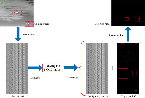
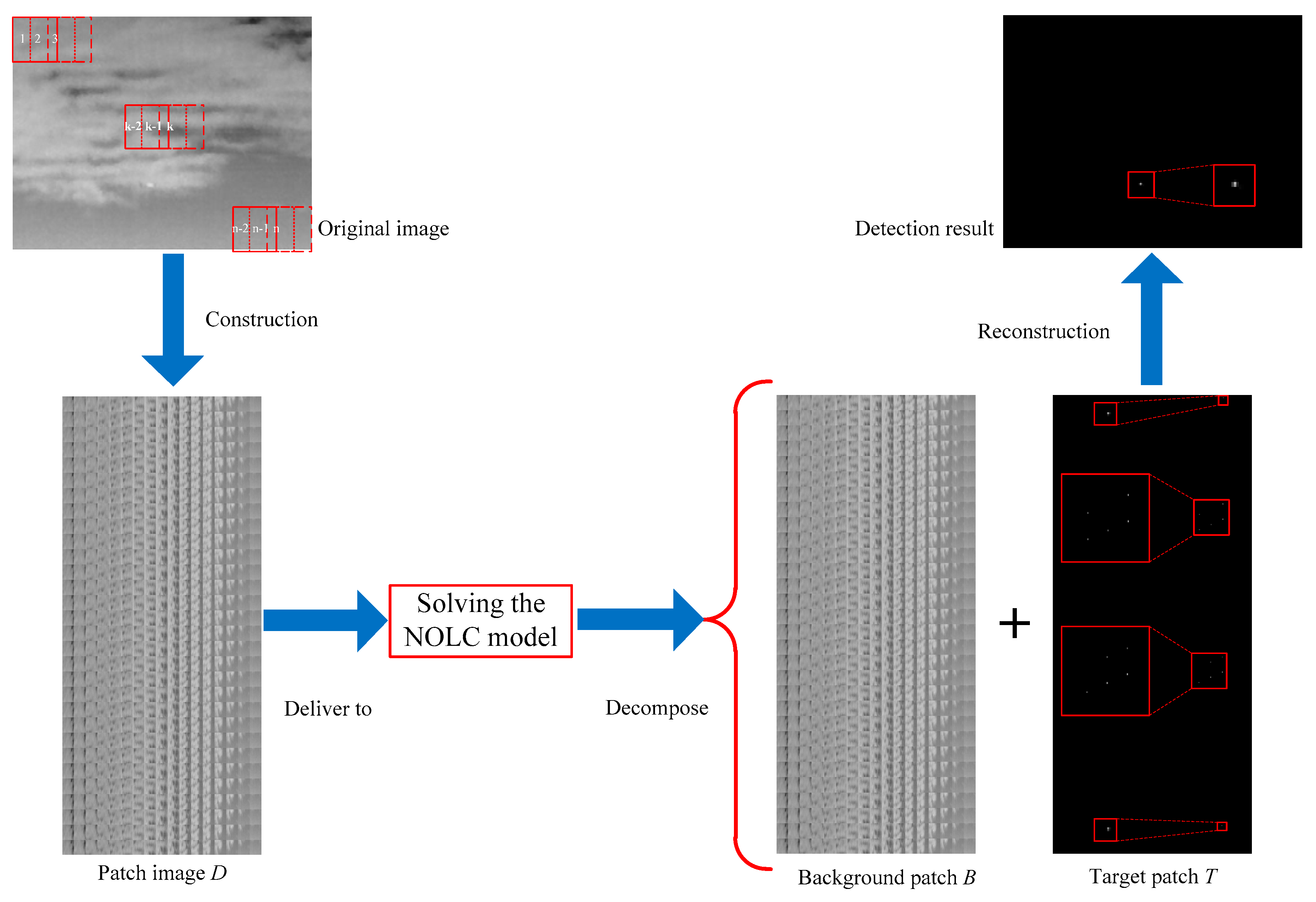
Here are the specific implementation steps for the NOLC method proposed in this paper. Figure 4 also shows the detection steps.

(a) Traversing an infrared image $I\left(x,y\right)$ using a sliding window of length len and a step size into the patch image $D\left(x,y\right)$; the values of these two parameters will be discussed in detail in Section 3.

(b) Initialize some parameters: $lambda=L/\sqrt{\max \left(size\left(D\right)\right)}$, the value of L and p will be discussed in Section 3; the recommended setting here is 1 and 0.4;

(c) Enter patch image $D\left(x,y\right)$ into Algorithm 1, and solve the target patch image $T\left(x,y\right)$ iteratively. It is worth mentioning that during the experiment we found that the non-zero elements in the target patch image no longer increase before the algorithm converges. In order to speed up the convergence of the algorithm, we set the non-zero element to no longer to increase as one of the conditions for the algorithm to stop iterating;

(d) Restore the target image $t\left(x,y\right)$ with the same sliding window as step (a);

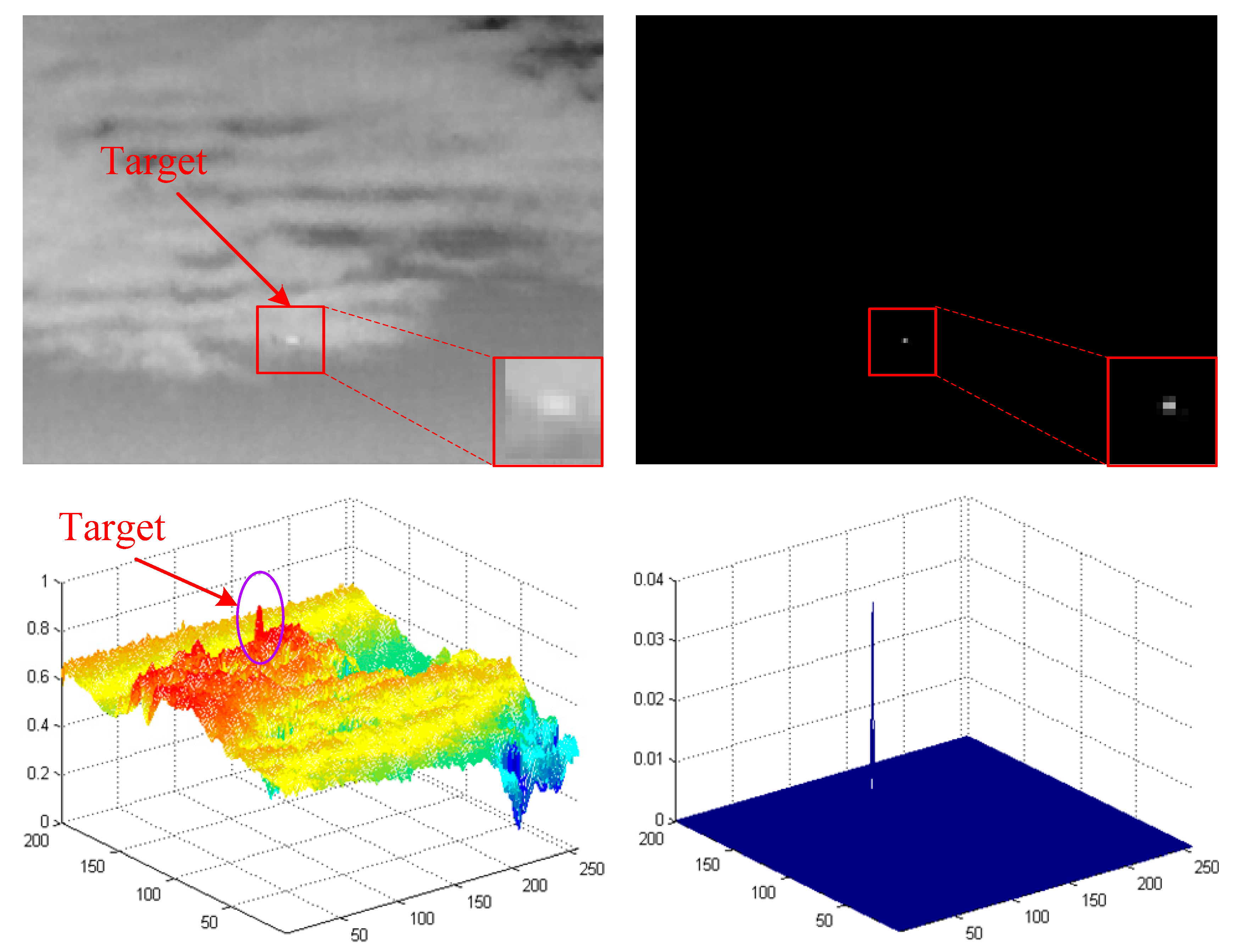
(e) Threshold segmentation to the target image using the following formula, where $th$ is the threshold for segmentation; $\mu$ and $\sigma$ represents the respective mean and variance of the target image. Figure 5 shows the detection result of NOLC model.

$$th=\mu +k\ast \sigma$$

(23)

3. Experiments

In this section we will introduce the evaluation indicators of this paper, discuss the impact of different parameter settings on the NOLC model, and compare NOLC with state-of-the-art, and finally, verify the validity of the NOLC model through the above steps.

3.1. Experimental Setting

This paper compares the NOLC model to the Tophat method (Tophat), Max Median method (MaxMedian), Local Contrast Method (LCM), Multiscale Patch-based Contrast Measure (MPCM), Infrared Patch Image (IPI) model and Reweighted Infrared Patch Tensor (RIPT) model, Non-Convex Rank Approximation Minimization (NRAM). The algorithm parameter settings used in this paper are given in

Table 1. Algorithm parameter setting.

Algorithm Name	Abbreviation	Parameter Setting
Tophat Method	Tophat	Structure shape: disk Structure size: $5\times 5$
Max Median Method	MaxMedian	Support size: $5\times 5$
Local Contrast Method	LCM	Window radius: 1,2,3,4
Multiscale Patch-based Contrast Measure	MPCM	Window radius: 1,2,3,4
Infrared Patch Image model	IPI	Patch size: $30\times 30$ Slide step: 10, L: 1 Lambda: $L/\sqrt{\min (m,n)}$
Reweighted Infrared Patch Tensor model	RIPT	Patch size: $30\times 30$ Slide step: 10, L: 1 Lambda: $L/\sqrt{\min (I,J,P)}$ h: 10, $\epsilon$: 0.01
Non-Convex Rank Approximation Minimization	NRAM	Patch size: $30\times 30$ Slide step: 10, L: 1 Lambda: $L/\sqrt{\min \left(m,n\right)}$
Non-Convex Optimization with Lp-Norm Constraint	NOLC	Patch size: $30\times 30$ Slide step: 10 Lambda: $L/\sqrt{\max \left(size\left(D\right)\right)}$ L: 1, p: 0.5

. In addition, the specific information and image descriptions of the four sequences tested in this paper are summarized in

Table 2. Test sequence information.

Sequence	Resolution	Image Description
Seq1	$256\times 200$	The target is a long strip, the target is relatively pure, but there is a lot of horizontal cloud interference above the image.
Seq2	$320\times 240$	The target is close to a circle with noise interference around it, and there are a lot of irregular clouds at the edges of the image.
Seq3	$256\times 172$	The target is relatively bright, and it shuttles through the clouds. There are a lot of structural disturbances around it. At the same time, the target changes greatly in the field of view, and the background changes quickly.
Seq4	$252\times 213$	The target occupies a small number of pixels, and there is vertical clutter interference around the target, there is cluttered grass under the image, and the brightness around the target is uneven.

. The software used in this article is MATLAB R2014a and the CPU is Core i5 7500, 3.4 GHz.

In order to objectively illustrate the effectiveness of the NOLC method, this paper uses quantitative evaluation indicators such as the receiver operating characteristic (ROC) curve, signal-to-clutter ratio gain (SCR Gain), background suppression factor (BSF) and iteration number.

(a) ROC curve

The ROC curve is widely used in the evaluation of two-class models and also in the field of infrared small target detection. It can quantitatively describe the dynamic relationship between the true positive rate (TPR) and false positive rate (FPR), and give neutral and objective suggestions when evaluating algorithms. The abscissa of the ROC curve is TPR, which reflects the proportion of the target being correctly detected; the ordinate is FPR, which reflects the proportion of non-targets being misdetected as targets. Therefore, the closer the ROC curve is to the upper left corner, the better the algorithm works. When the ROC curve is applied to infrared small target detection, the abscissa and ordinate are defined as follows:

$$\mathrm{FPR}=\frac{\%\mathrm{number}\mathrm{of}\mathrm{pixels}\mathrm{detected}\mathrm{in}\mathrm{background}\mathrm{region}}{\%\mathrm{real}\mathrm{targets}}$$

(24)

$$\mathrm{TPR}=\frac{\%\mathrm{real}\mathrm{targets}\mathrm{detected}}{\%\mathrm{real}\mathrm{targets}}$$

(25)

Another key indicator of the ROC curve is the area under the curve (AUC). In general, the larger the AUC, the better the algorithm works.

(b) SCR Gain and BSF

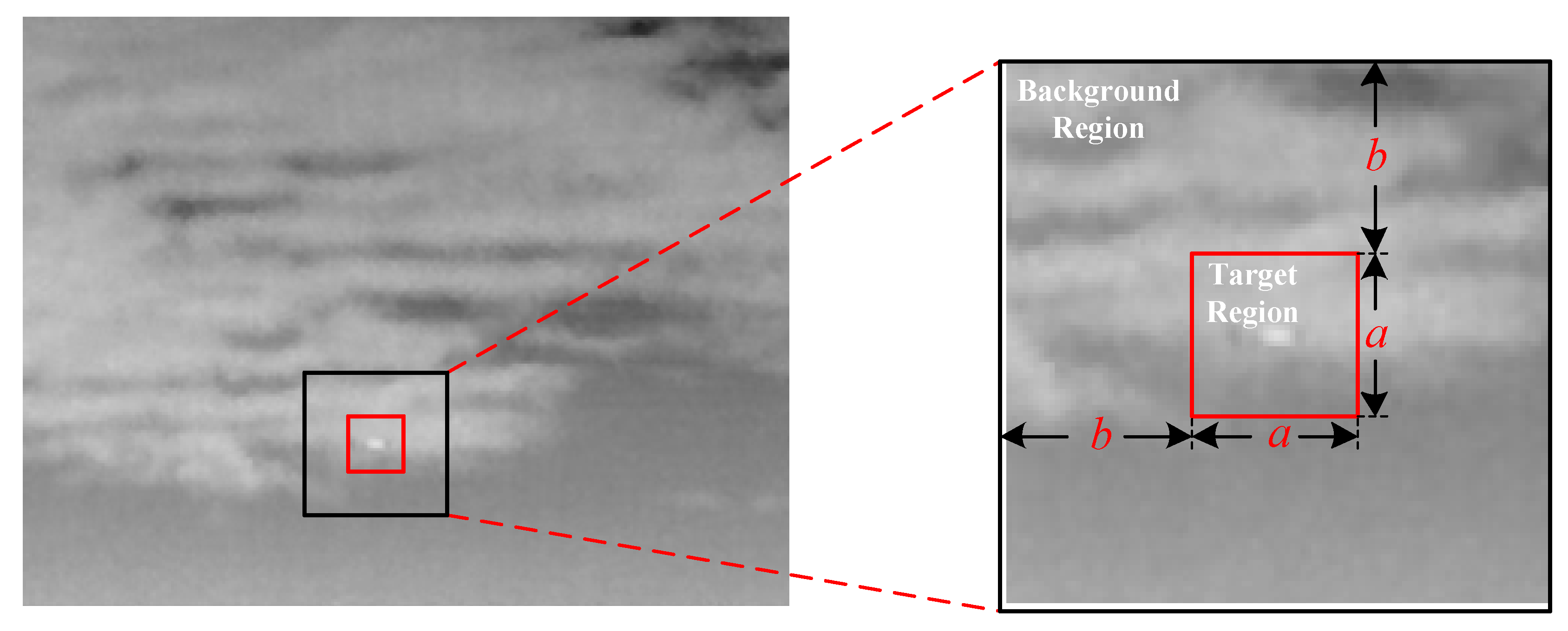
SCR Gain and BSF are indicators for measuring the degree of improvement of the target and the ability to suppress the background, respectively. Their definition of the target and background area is shown in Figure 6, defined as Equation (26).

$$\mathrm{SCRG}=\frac{{(S/C)}_{out}}{{(S/C)}_{in}},\mathrm{BSF}=\frac{C_{in}}{C_{out}}$$

(26)

where S and C denote the signal (target region) amplitude and clutter (background region) standard deviation, respectively; in and out represent the original image and the detection result image. In the experiment, the values of a and b are 10 and 40, respectively. According to the definition, the larger the values of SCR Gain and BSF, the better the detection performance of the algorithm.

(c) Iteration number

All the sparse and low-rank matrices recovery based methods involve iterative solution, in which the iteration number of the algorithm directly affects the detection efficiency and running time. If a method has fewer iterations, it basically shows that the operation time is shorter, so the iteration number is also a key evaluation indicator.

3.2. Algorithm Validity

This section will prove the robustness of the NOLC model in various scenarios from the scene validity, and compare the proposed model with the IPI model and NOSLC model to prove the feasibility of NOLC.

(a) Validity of Diverse Scene

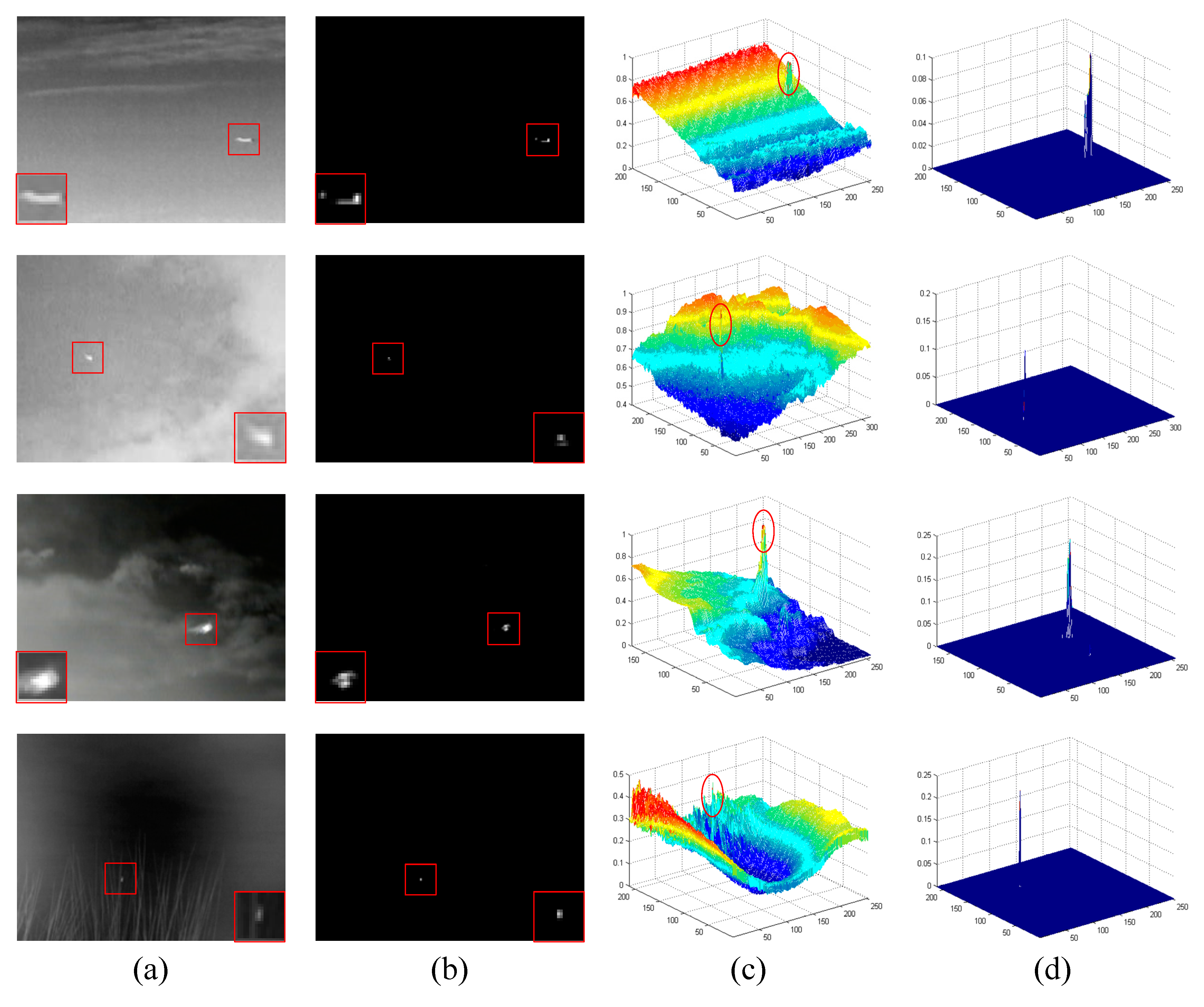
The NOLC model strengthens the constraint on sparse items, and at the same time appropriately shrinks the constraints on low rank items, so it has a good detection effect. Figure 7 shows multiple original images, NOLC processing results, and their three-dimensional display.

In order to better display the target information, the target region in the Figure 7 is enlarged and placed in the corner of the image. Each row in Figure 7 represents the presentation of the images in Sequence 1–4, with each column being the original image, NOLC processing results and their three-dimensional display. It can be seen from the Figure 7 that NOLC can accurately detect small targets regardless of whether the background is submerged in the clutter or the gray scale of the image is not uniform. As far as the result is concerned, the detected target image has only a corresponding target position, and the background region is suppressed to 0, so the effect of NOLC is remarkable.

(b) Validity of the Proposed Algorithm

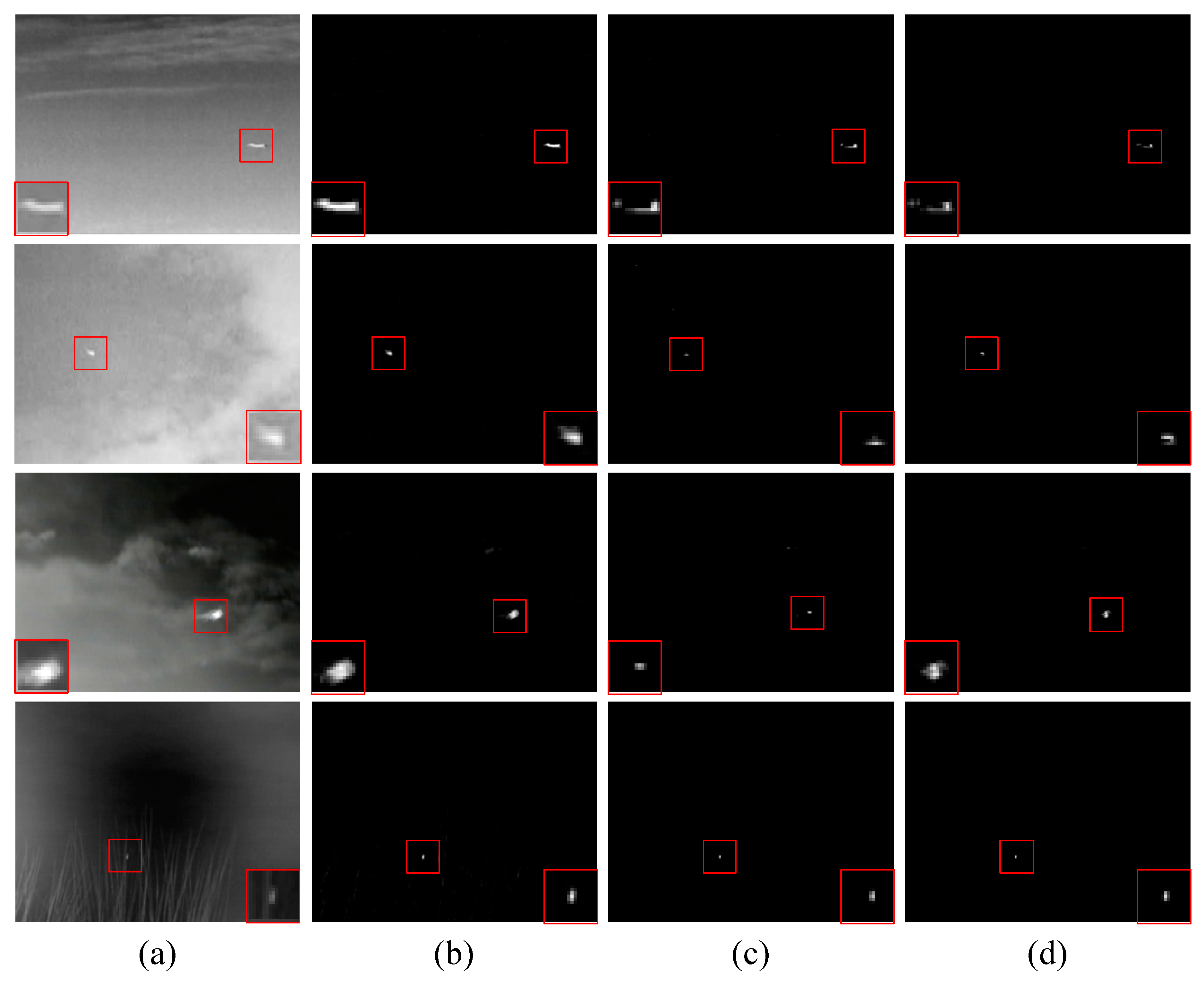
The previous section verifies that NOLC is effective. This section compares it with the IPI and NOSLC model mentioned in this paper, and the effectiveness of this method will be further confirmed. Figure 8 and Figure 9 show the results of the three algorithms.

In Figure 8, from left to right are the original image, IPI, NOSLC and NOLC result image and from top to bottom are sequences 1–4. Similar to Figure 7, the target region is placed in the corner of the image in the processing result. For better illustration, Figure 9 shows a three-dimensional view of the corresponding position image of Figure 8. In the figure, the target position in the original image is circled in red, and the position of the clutter is circled with cyan in the 3D display of processing result. Since the clutter is relatively small in 3D display, it is not easy to visually see it, so it is marked in a cyan circle. It can be seen from the figure that all three methods can detect the target, but the IPI method contains much clutter when dealing with complex background images. The results of the NOSLC method are relatively low in terms of clutter, but because the constraints on the background low rank are stricter, the result is not very satisfactory. The NOLC method enhances the sparsity of the target and appropriately scales the background low rank property. The result is the lowest among the three methods in terms of clutter, and the background of most images is suppressed to 0. The test results of the sequence images are shown in Figure 10.

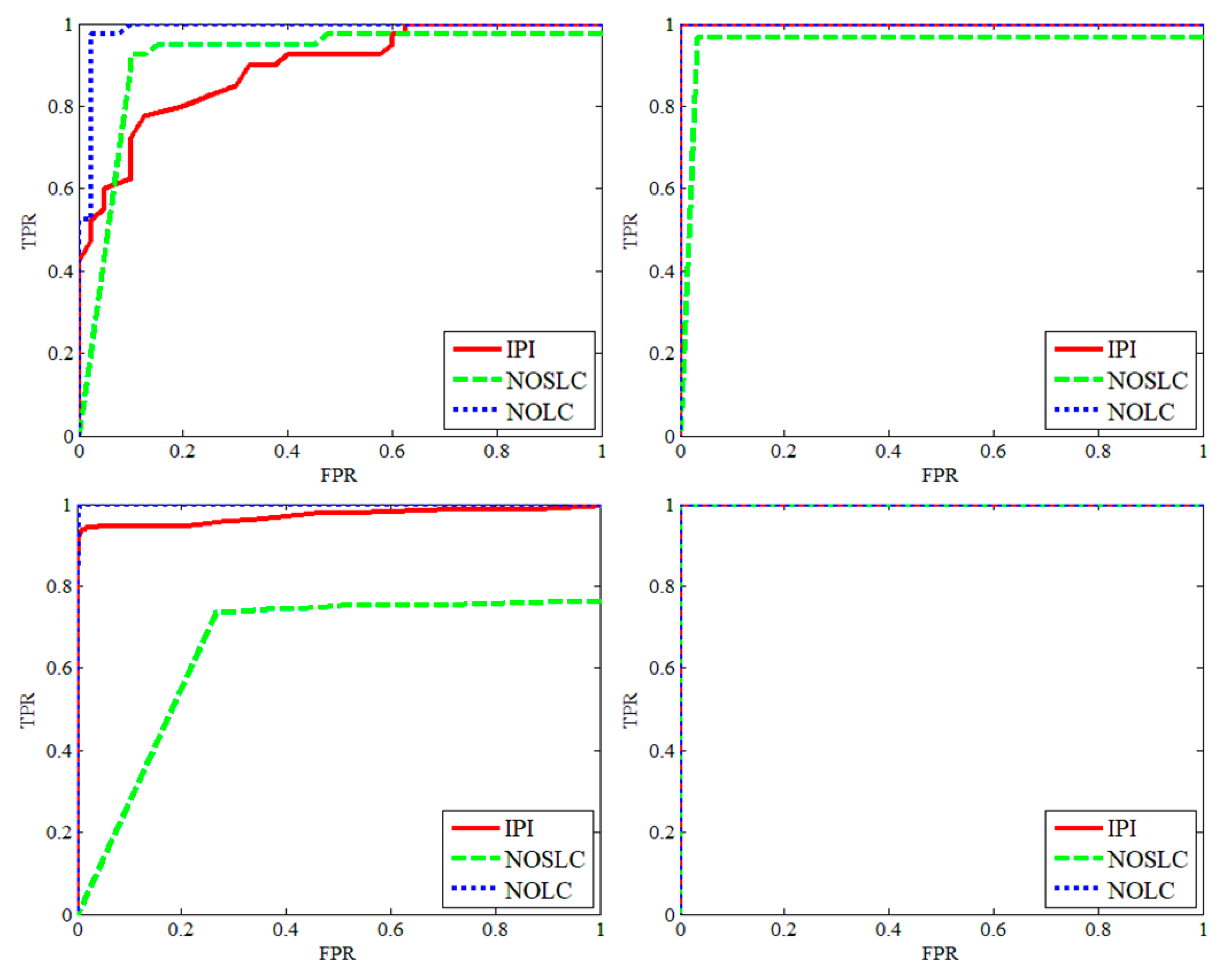
From the upper left corner to the lower right corner in Figure 10 are sequences 1–4. It can be seen that the three algorithms in Seq 4 have similar effects. The NOLC and IPI effects in Seq 2 are comparable and superior to NOSLC. In Seq 1, 3 the FPR of NOLC rises to 1 at the fastest, which is better than the other two. According to the above analysis, NOLC can not only accurately detect infrared small targets, but is also better than the IPI method and NOSLC method designed in this paper.

3.3. Parameter Analysis

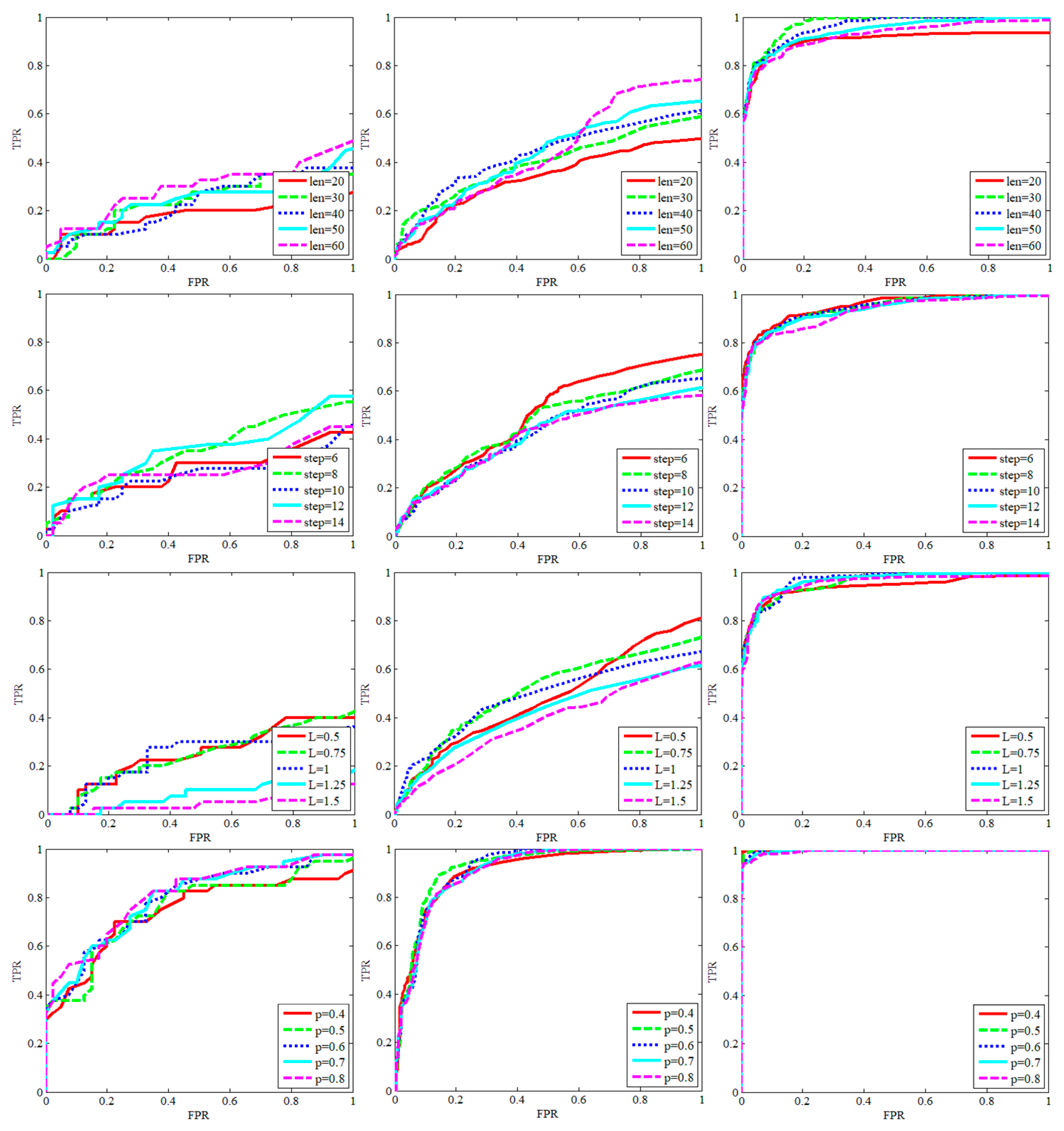
In this section, we compare the four key parameters of NOLC to discuss the effect of parameter settings on the detection of NOLC method. The four parameters are the sliding window size len, the window sliding step size step, the Lambda initialization parameter L and the value of p in the Lp-norm. Figure 11 shows the ROC curve for comparison of these parameters.

The three columns from left to right in Figure 11 represent the ROC comparison chart of sequence 1–3, respectively. From top to bottom, the ROC curve comparison of the sliding window size len, sliding step, L and p parameters is shown. In the comparison experiment of the sliding window size len, we set the len values to 20, 30, 40, 50 and 60, and the remaining parameters are consistent. For qualitative considerations, if the len value is small, then the elements of each column in the patch image D will be relatively small, and the information contained will be less, the association between the columns will be missing, and the low rank and sparsity cannot be accurately guaranteed. On the contrary, if the len value is relatively large, it will not strictly conform to the constraint due to too many elements and redundant information. The first row of the ROC curve in Figure 11 also illustrates this. In the figure, when the len value is 30, a good ROC performance can be maintained in more sequences, and thus the len value can be taken as 30.

For the sliding window step, the step value is smaller, the window change is smaller each time, and the low rank property is stronger, but the small step greatly increases the block image matrix dimension and affects the algorithm detection efficiency. The second row in Figure 11 shows the ROC contrast image with step values of 6, 8, 10, 12, 14 when the remaining parameters are unchanged. In order to achieve a balance between algorithm efficiency and detection efficiency, the step value is recommended to be 10. In addition, the value of L also affects the detection effect. The third row in Figure 11 shows the ROC contrast image with different L values. It can be seen from the figure that the ROC curve performs best when the value of L is 1.

The fourth row of Figure 11 shows the ROC comparison of the last key parameter p. As mentioned in the second section, the smaller the p, the stronger the constraint on the low rank property and the efficiency of the algorithm is guaranteed. But when p is too small, the target cannot be detected. When the p value is increased, although the detection accuracy of the target can be ensured, it will increase the calculation time. Therefore, the choice of p value should be as small as possible. In combination with the ROC curve comparison in Figure 11, the p value is recommended to be 0.4.

3.4. Comparison to State-of-the-Art

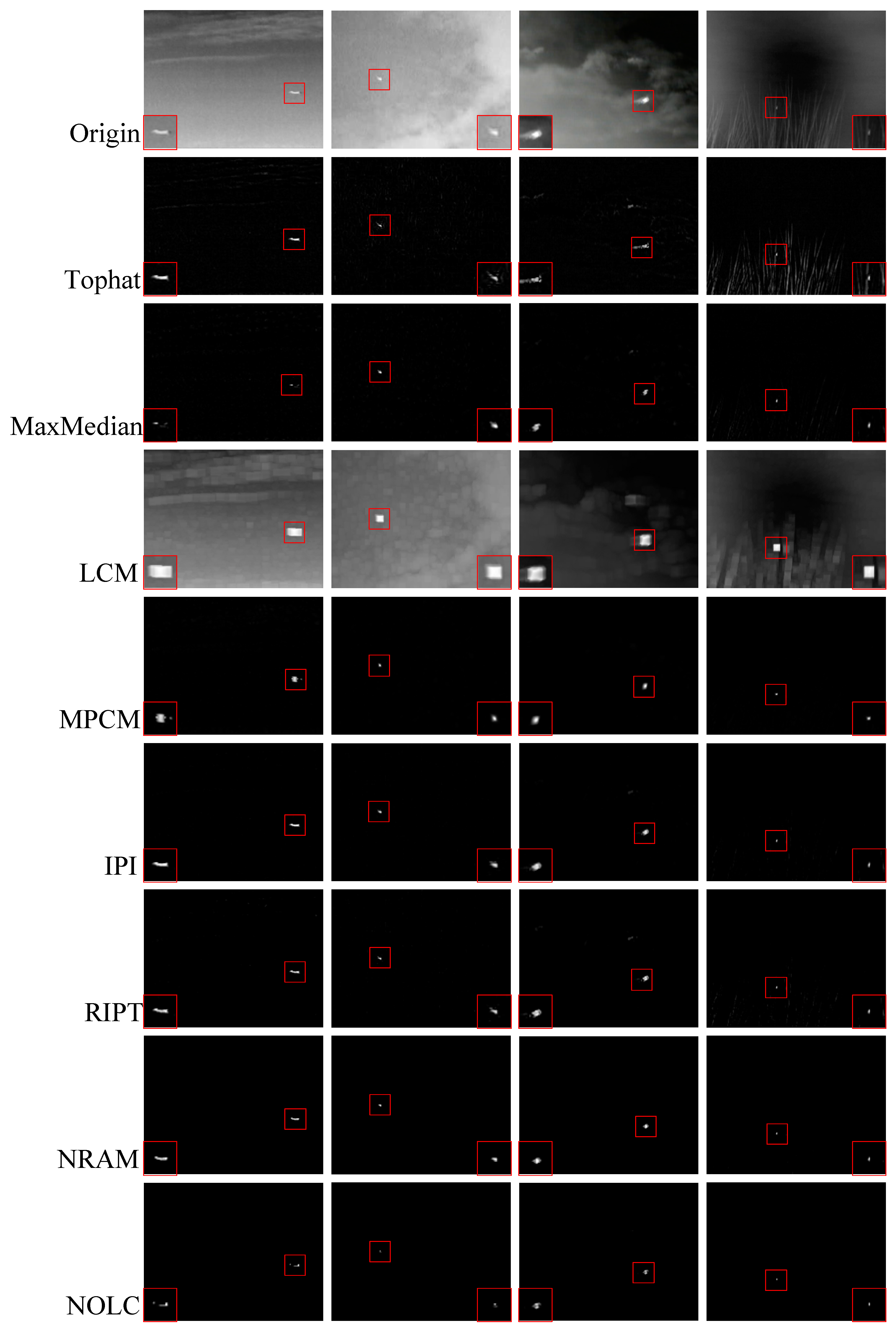
The above sections verify the effectiveness of the diverse scene and the proposed method, and discuss the setting of key parameters. In this section, we compare the NOLC algorithm with other detection algorithms. The parameter settings of the seven contrasting algorithms and NOLC are presented in Table 1. We compared the NOLC model to the Tophat method (Tophat), Max Median method (MaxMedian), Local Contrast Method (LCM), Multiscale Patch-based Contrast Measure (MPCM), Infrared Patch Image (IPI) model, Reweighted Infrared Patch Tensor (RIPT) model and Non-Convex Rank Approximation Minimization (NRAM). The effect of all algorithms on a single frame image is shown in Figure 12 and Figure 13.

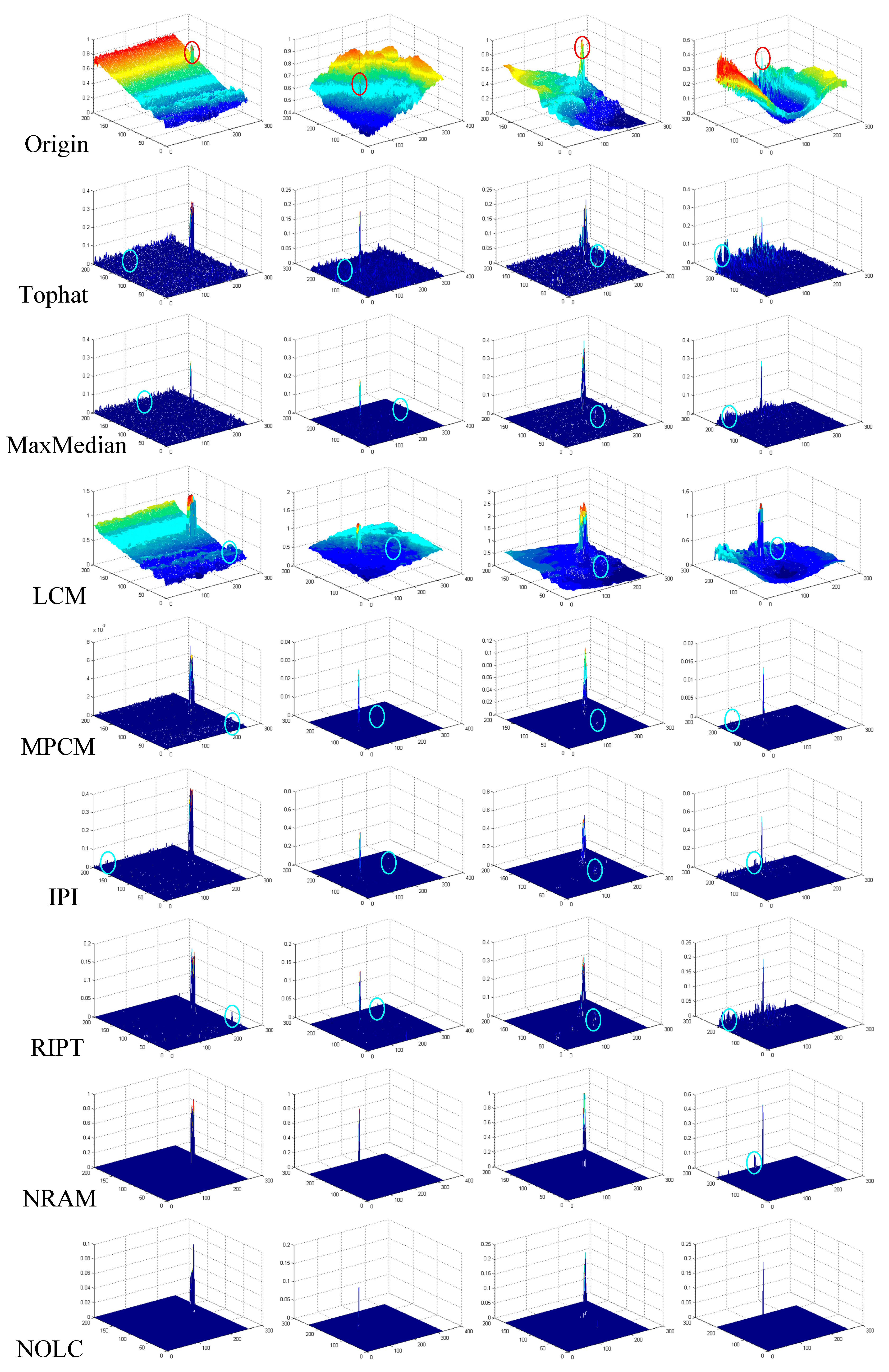
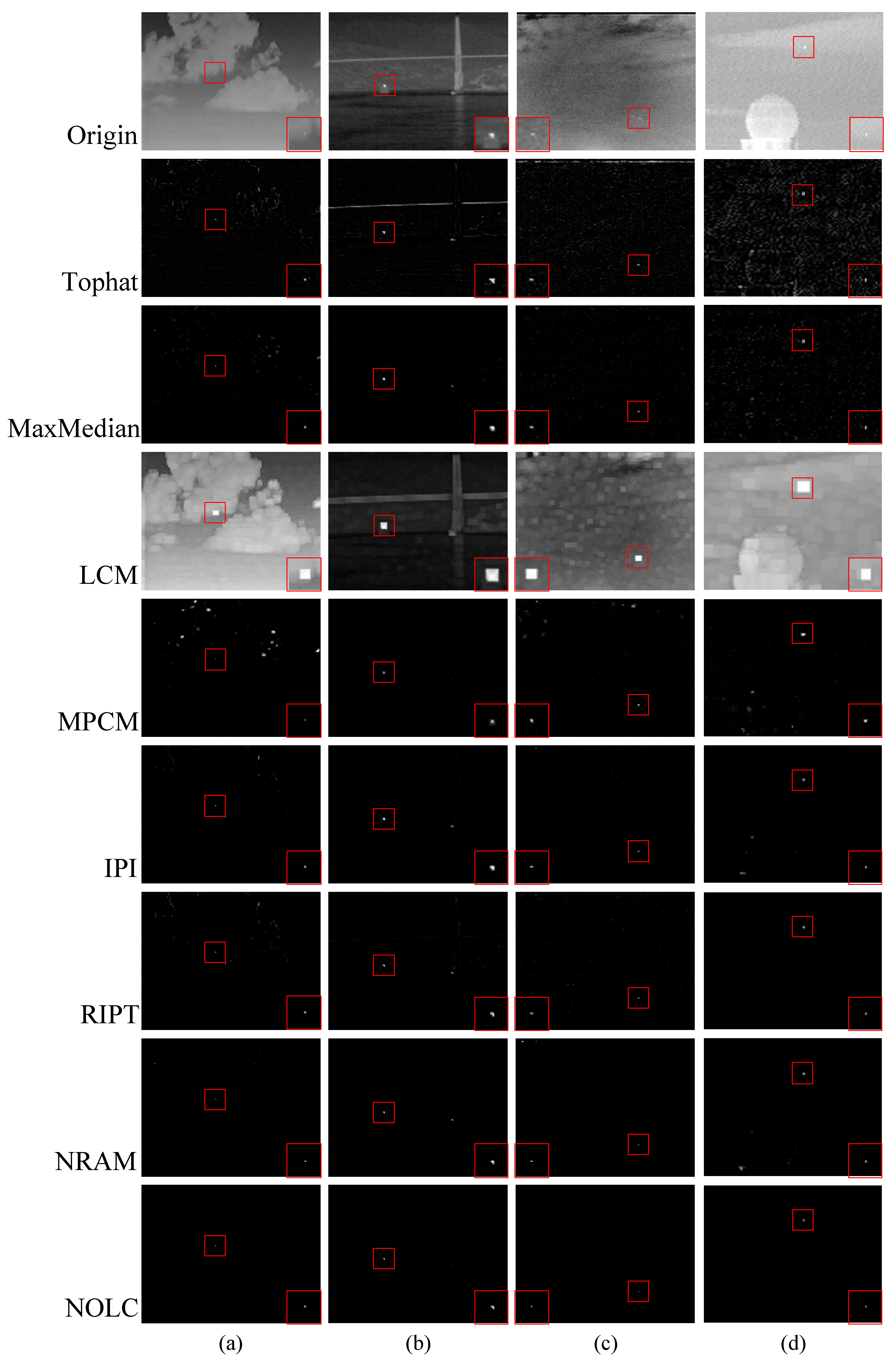
Figure 12 shows the processing results of the original image and the above seven algorithms. For better display, the target region is framed in red and enlarged to the corner of the image. Figure 13 is a 3D representation of the corresponding position image of Figure 12. As in the previous section, the target position in the original image is circled in red, and the position of the clutter is circled in cyan in the 3D display of processing result.

In the above method, Tophat and MaxMedian are classic infrared small target detection methods. It can be seen that Tophat has a lot of clutter, while MaxMedian has less relative clutter but the target is greatly weakened. LCM and MPCM are typical methods based on the HVS method, but because the processing mechanism of LCM is relatively simple, the effect is not ideal. MPCM is able to accurately detect the target, but there is still a significant clutter in Sequence 1. IPI, RIPT, NRAM and NOLC are all sparse and low-rank matrices recovery based methods. Both IPI and RIPT can observe obvious clutter and have poor robustness. NRAM and NOLC can accurately detect the target while keeping the background basically suppressed to zero. However, as shown in the figure, the NRAM processing result has significant clutter.

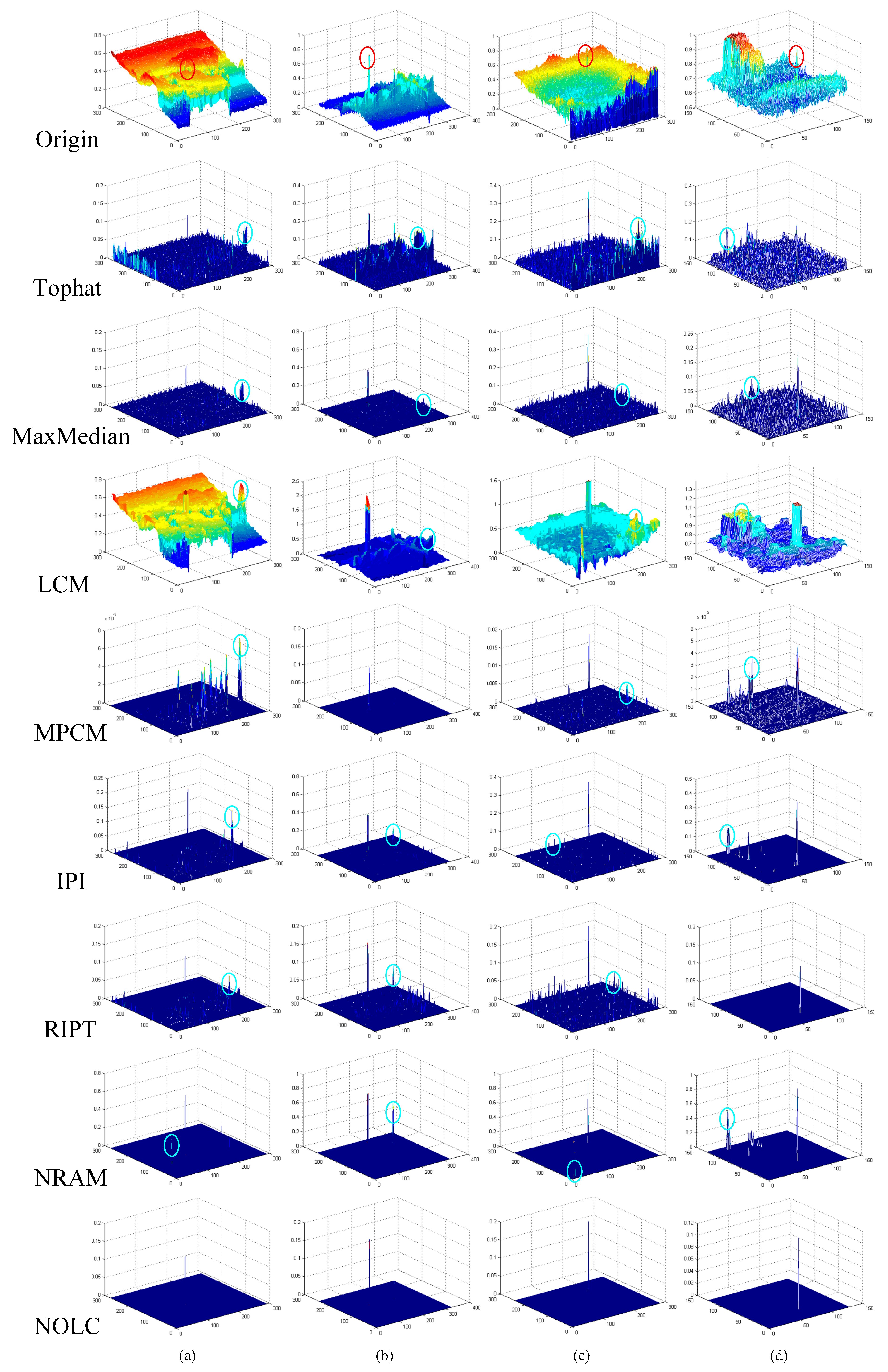
To further demonstrate the superior performance of the NOLC method, we have experimented with four other complex scenarios. The processing results are shown in Figure 14 and Figure 15 and the marking method is the same as above. The target position in the original image is circled in red, and the position of the clutter is circled in cyan in the 3D display of the processing result. The background of scene 1 is a large number of clouds, and the target occupies very few pixels and is disturbed by the clouds; scene 2 is a sea-sky background, in which there is sea level interference, and the bridge body appears as a structural disturbance in the picture, and the scene is very complicated; scene 3 is an air background, and irregular clouds appear on the edges. The image noise is relatively large, which also brings difficulty to the detection; the random noise in scene 4 is very strong, and there is a strong architectural disturbance in the lower left.

It can be seen from the experimental results that the background suppression based methods and the HVS based methods are very difficult to detect small targets in complex backgrounds. This is because the assumptions of the two methods are simple, and it is difficult to distinguish between clutter and target when encountering complex backgrounds. In contrast, because the assumptions of the sparse and low-rank matrices recovery based methods are supported by scientific physical models, they are superior in effect to other kinds of algorithms. However, there is still a lot of clutter in the processing results of IPI and RIPT. This is because the IPI model only limits the sparse item to a rough one, resulting in poor detection results. The RIPT method uses structural tensors to weight the sparse item, and the sparse constraints are still not strict, so the detection effect of RIPT is not ideal. As for the NRAM method, since the method only imposes constraints on the clutter, the contribution of this constraint to the detection effect is indirect, and the sparsity of the target is not strictly limited, so there is still clutter in the complex background. The NOLC method directly strengthens sparsely constrains and thus always finds sparse target locations in complex backgrounds, which explains why NOLC processing results have little clutter. This experiment also preliminarily illustrates the excellent robustness of NOLC.

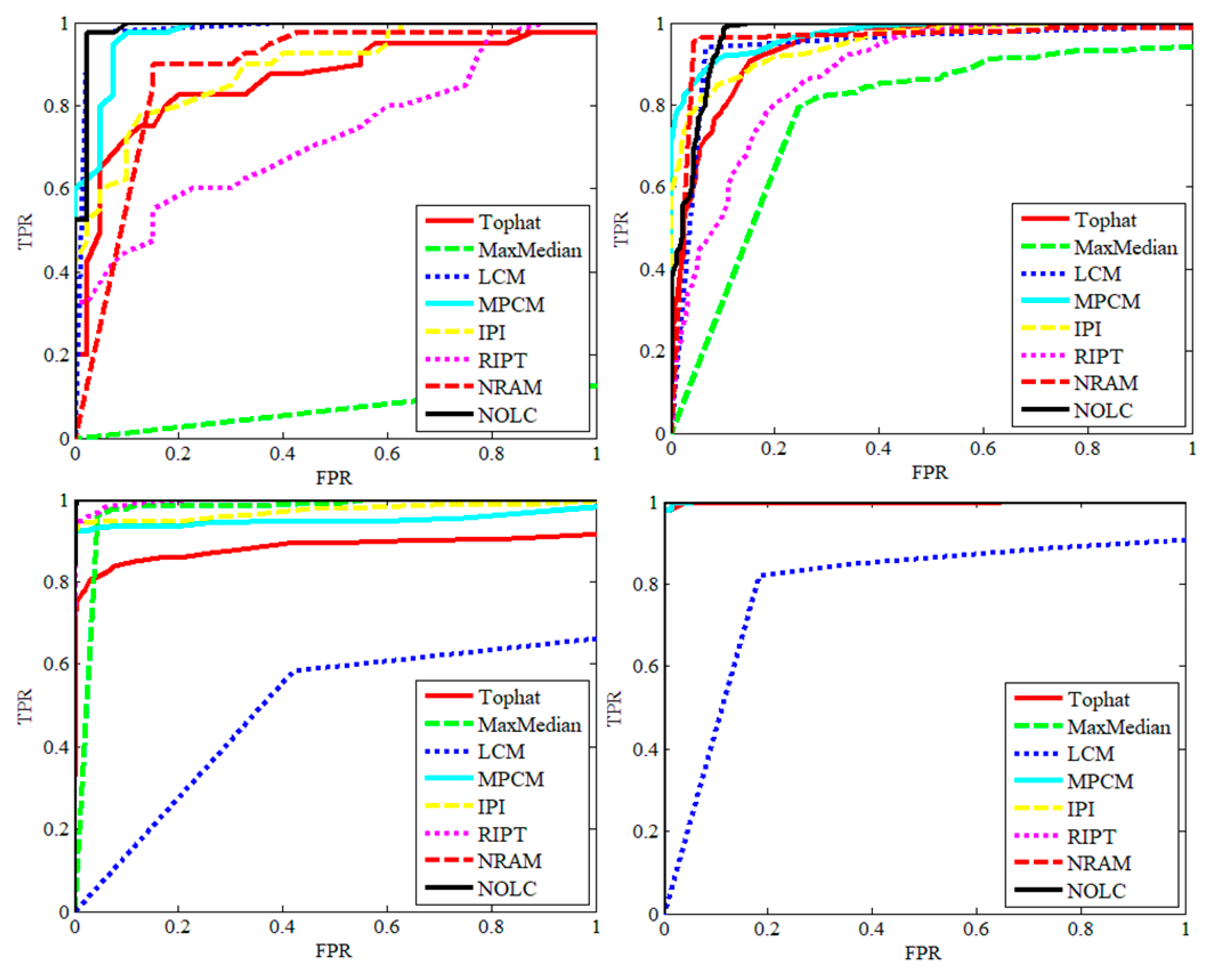
The ROC comparison chart for the seven algorithms for the above four sequences is given by Figure 16 where the black line represents the curve of NOLC. From the top left to the bottom right, they represent sequences 1–4. As can be seen from the figure, the NOLC curve can always achieve a TPR of 1 when the FPR is relatively small, which means that the AUC of the NOLC is larger. To better compare the AUC of each of the curves in Figure 16, their specific values are listed in

Table 3. AUC of the ROC curves in Figure 14.

	Seq1	Seq2	Seq3	Seq4
Tophat	0.8591	0.9384	0.8814	0.9974
MaxMedian	0.0688	0.7698	0.9679	1.0000
LCM	0.9828	0.9369	0.4835	0.7855
MPCM	0.9731	0.9712	0.9494	0.9996
IPI	0.8900	0.9489	0.9721	1.0000
RIPT	0.7256	0.8781	0.9959	1.0000
NRAM	0.8769	0.9535	1.0000	1.0000
NOLC	0.9866	0.9657	0.9996	1.0000

Note: The maximum value of each sequence AUC is indicated in red and the second largest value is indicated in purple.

, where the maximum value of each sequence AUC is indicated in red and the second largest value is indicated in purple. From Table 3 we can quantitatively observe that the AUC of NOLC is the second largest in Sequence 2 and 3, and the rest are the largest. Therefore, it can be said that NOLC's performance in the sequence image test is remarkable.

The test data for the other two key evaluation indicators, SCR Gain and BSF, are listed in

Table 4. Comparison of SCRG and BSF in various methods.

	Seq1		Seq2		Seq3		Seq4
Evaluation Indicators	SCR Gain	BSF	SCR Gain	BSF	SCR Gain	BSF	SCR Gain	BSF
Tophat	10.78	5.196	3.936	2.764	11.68	14.62	2.451	1.864
MaxMedian	0.850	3.237	3.975	2.092	4.882	12.18	3.638	2.643
LCM	3.047	1.575	2.742	1.772	6.007	6.428	7.524	5.806
MPCM	102.2	111.3	193.8	138.9	Inf	Inf	129.1	116.9
IPI	121.3	53.50	48.06	25.19	218.5	190.6	22.10	12.80
RIPT	122.7	68.44	Inf	Inf	Inf	Inf	12.97	9.929
NRAM	Inf	Inf	Inf	Inf	Inf	Inf	Inf	Inf
NOLC	Inf	Inf	Inf	Inf	Inf	Inf	Inf	Inf

Note: The maximum value is indicated in red and the second largest is indicated in purple.

. Similarly, the maximum value is indicated in red and the second largest is indicated in purple. You can see that the two classic methods do not perform very well. In the HVS based method, MPCM performs excellently with two maximum values and five second largest values. In the sparse and low-rank matrices recovery based methods, in addition to NOLC, the performance of RIPT is also excellent, with four maximum values and one second largest value. Overall, the comparison of the eight algorithms of NRAM and NOLC has the upper hand and has a maximum in each sequence. This shows that the two methods also do a better job of suppressing the background.

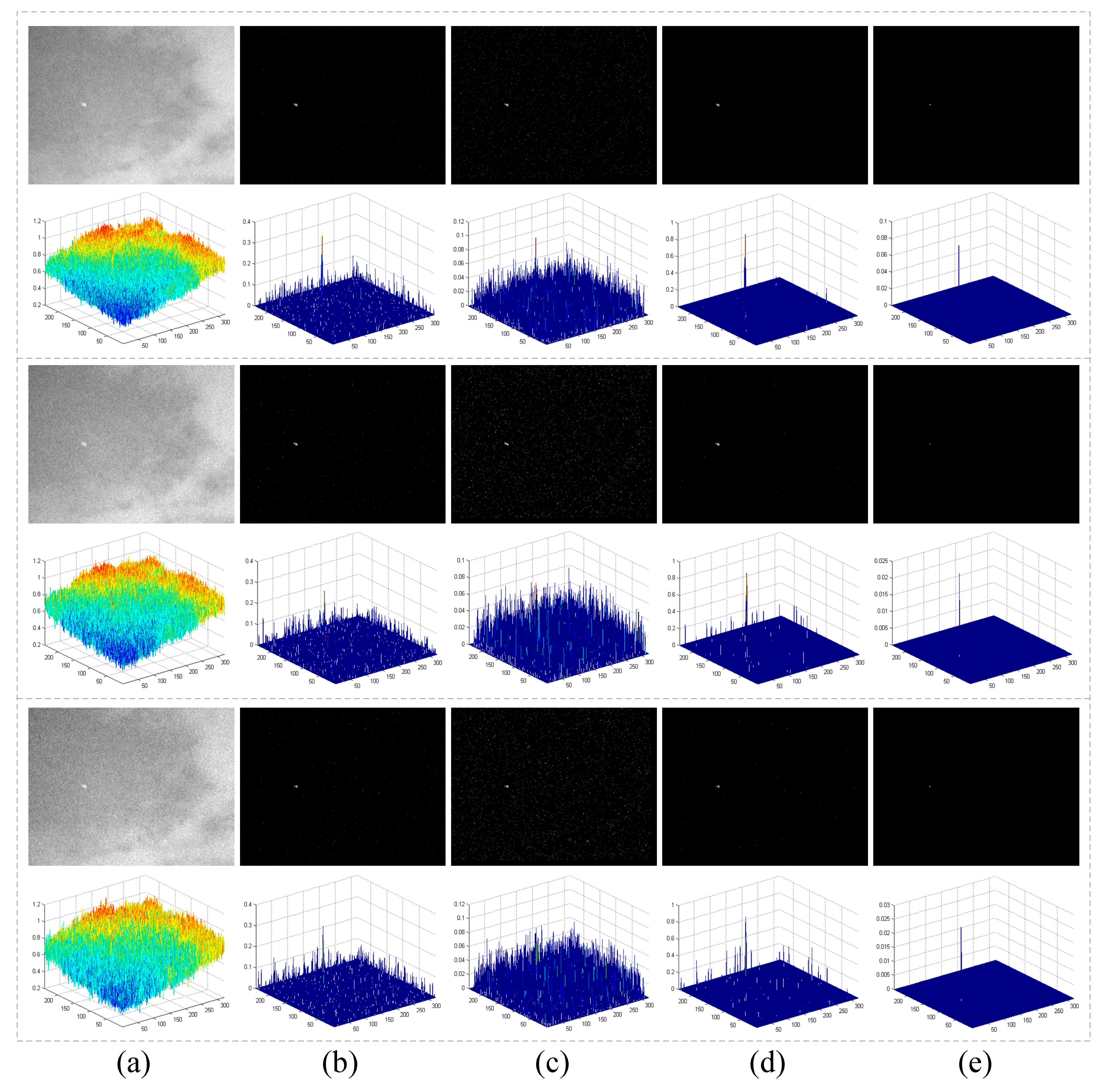
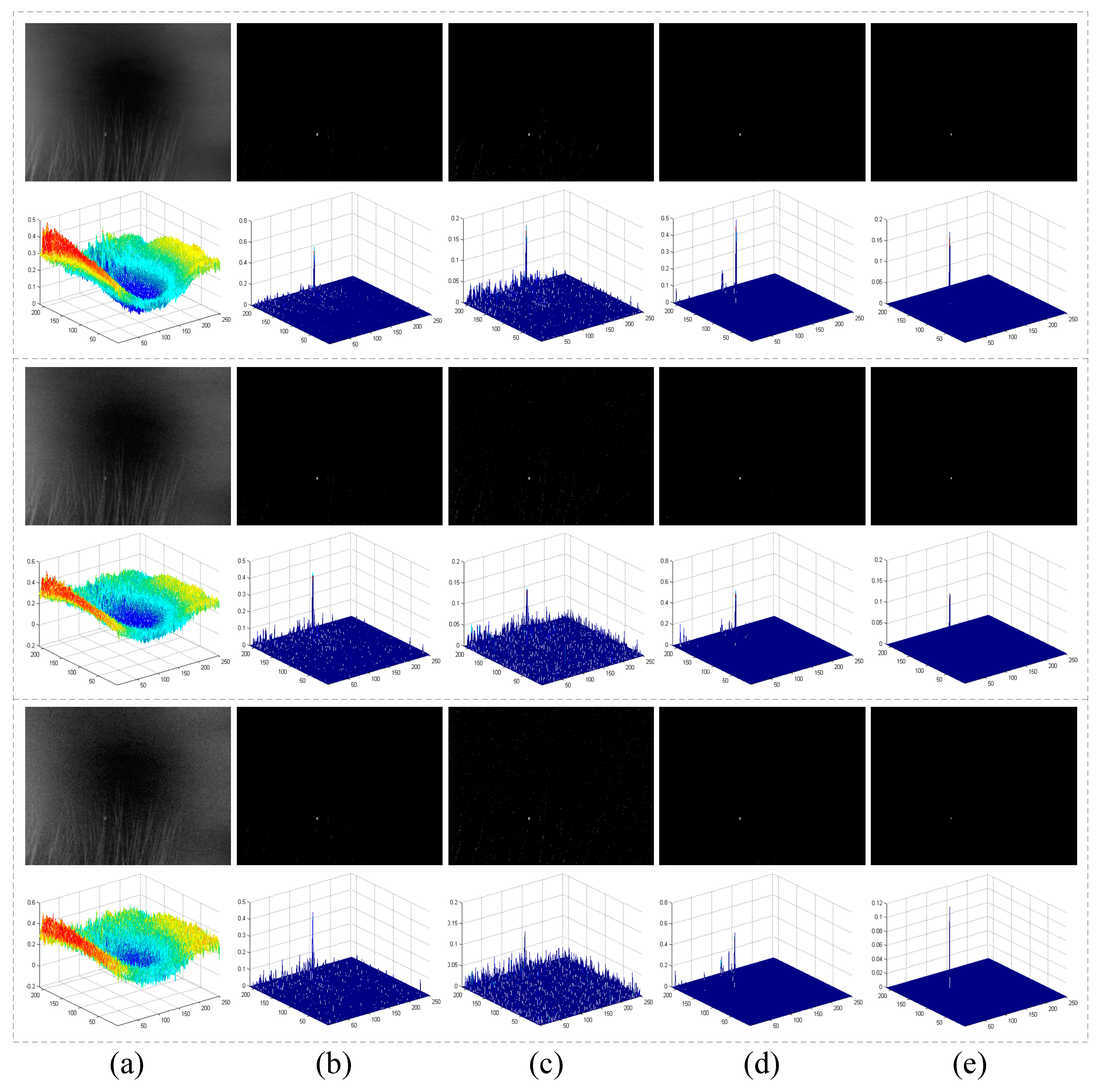
To further illustrate that the performance of the NOLC method is superior to the rest of the methods while verifying its robustness, we add normal noise with a mean of zero to the two sequences and compare it with IPI, RIPT and NRAM. The variance of the normal noise in Figure 17 is 0.04, 0.05 and 0.06. It can be seen that both IPI and RIPT are sensitive to noise, and the noise is very strong in the processing result. In the process of increasing the variance of the noise, the NRAM processing result is also mixed with a lot of clutter. While NOLC has always shown good performance, it can accurately detect the target and suppress the background very purely when the variance becomes larger. Figure 18 also illustrates the same fact in Seq 4. The above experiments show that the NOLC method is superior to other algorithms in terms of detection accuracy and algorithm robustness.

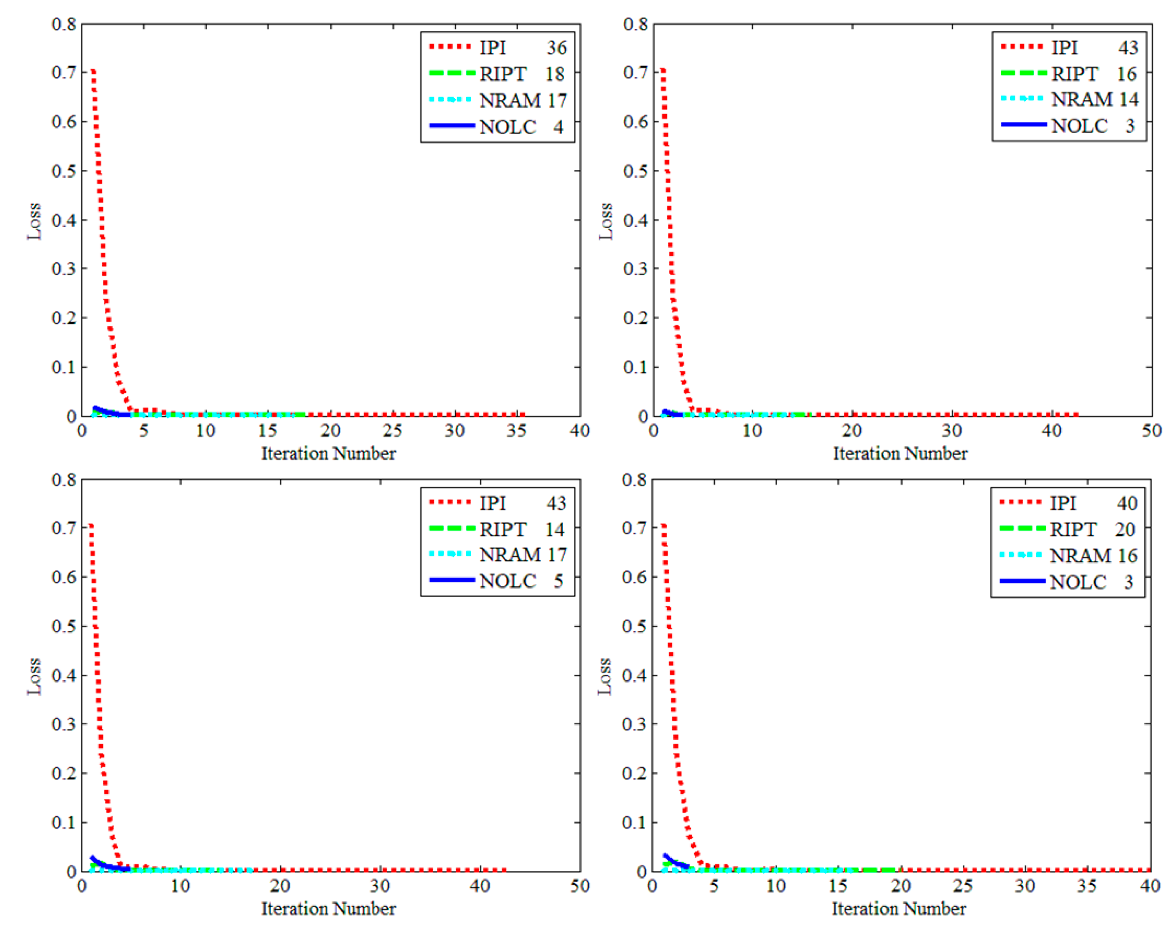
The last evaluation indicator is the iteration number. Since other methods do not involve iterative solution, four methods of IPI, RIPT, NRAM and NOLC are compared here. Figure 19 shows the iteration curves of the four methods in four sequences, where the algorithm name and the iteration number are given in the legend. It can be seen that since the IPI is solved by the accelerated proximal gradient (APG) method, the number of iterations is the highest, while RIPT and NRAM are solved by the faster ADMM method, and the iteration number is still higher than 10. The NOLC method not only uses the Lp-norm which can converge faster, but also improves the convergence judgment mechanism, so it can basically converge within 5 iterations. The convergence speed of NOLC is much better than the similar method, and it also has more advantages in running time.

In the experiments in this section, we show the detection effect of NOLC, and demonstrate the feasibility of NOLC by comparing IPI, NOSLC and NOLC. Then, in the aspects of the single frame effect, ROC curve, AUC, SCR Gain and BSF, the NOLC and other infrared small target detection methods are compared. It can be seen that the detection effect of NOLC has great advantages. The comparison of the image plus noise further illustrates the robustness of the NOLC method. Finally, the iteration number of NOLC and other sparse low-rank matrix reconstruction based methods are compared. The advantage of NOLC is explained again from the efficiency of the algorithm. All in all, NOLC is an excellent infrared small target detection method in terms of detection effect and running time.

4. Discussion

The sparse and low-rank matrix recovery-based methods have been widely used by researchers, and a large number of methods are also applied to the field of infrared small target detection. However, starting from the IPI model, researchers often only pay attention to the use of additional constraint coefficients to improve the detection effect, while ignoring the difference in the sparse degree of low ranking items and sparse items in the infrared small target image. Experiments on six sets of actual data show that the sparsity degree difference between low-rank items and sparse terms is very large, even not within an order of magnitude, so it is unscientific to use only L1-norm constraints. Aiming at this property of infrared small target image, this paper uses the Lp-norm to constrain the sparse term and relaxes the constraint on the low ranking term, and the NOLC method is proposed.

Compared with other methods, the IPI model is the original method, and its principle and solution method are relatively simple. From the perspective of background characteristics, the RIPT model uses the local structure tensor as the penalty coefficient of the sparse term, in order to obtain a more accurate background. Because the results of local structure tensor are relatively rough and cannot be used as an ideal sparse penalty factor, RIPT does not work well in the face of complex backgrounds. The NRAM method is based on the structural noise and uses the L21-norm constraint. The L21-norm emphasizes that the row of the block image is sparse. To achieve this effect, the size of the structured noise must be smaller than the size of the sliding window to obtain the effect of row sparseness. However, for structured noise, its size often cannot meet the requirements (such as bridges and houses), which makes the NRAM using the L21-norm constrained noise term sometimes unconvincing. The NOLC method considers the difference between the target and the background sparsity from the perspective of the target, and directly uses the stricter Lp-norm to constrain the sparse item. This method can describe the target more directly and accurately than the IPI model and the NRAM method, can also obtain good detection effects under various complex backgrounds, and can always restore sparse targets in the noisy infrared small target image. The NOLC method improves the convergence strategy while utilizing the Lp-norm property, making the convergence speed better than other methods.

This article gives ample demonstration of the performance of NOLC through experiments. Firstly, the effect of the NOLC method in multiple scenarios is verified. Then, the key parameters in the method are analyzed and the values of the parameters are given. Then, compared with the existing methods, the results are also in line with the above analysis. NOLC is superior to other algorithms in detection accuracy, and can suppress most backgrounds to zero in terms of background suppression. Then, the noise infrared small target image is tested to verify the anti-noise ability of NOLC, and the robustness of the algorithm is further illustrated. Finally, comparing the iterative convergence speed of the four methods, NOLC also has obvious advantages.

In summary, the NOLC method has the advantages of high detection accuracy, anti-noise, fast convergence, etc. This method is not only a change of the metric, but an improvement of the performance brought by the improvement of the method. Recently, tensor-based infrared small target detection methods have also received extensive attention [34,55]. These method replace the matrix with tensor, and they can also provide good detection results.

5. Conclusions

In this paper, a novel infrared small target detection method based on non-convex optimization with Lp-norm constraint (NOLC) is proposed. The detection effect of the algorithm is enhanced by extending the original nuclear norm and L1-norm to the schatten q-norm and Lp-norm to strengthen the constraints on sparse items and appropriately scaling the constraints on low-rank items. At the same time, the NP-hard problem is transformed into a non-convex optimization problem. The NOLC model can not only accurately detect the target, but also greatly suppress the background area, achieving a good infrared small target detection effect. In the final part of the experiment, NOLC was compared with seven methods. It performed well on the ROC curve and also had very high SCR Gain and BSF. The comparison of the image plus noise further illustrates the robustness of the NOLC method. At the same time, it is also ahead of other algorithms in the number of iterations, which means that NOLC also leads in computing time.

References

- Shao, X.; Fan, H.; Lu, G.; Xu, J. An improved infrared dim and small target detection algorithm based on the contrast mechanism of human visual system. Infrared Phys. Technol. 2012, 55, 403–408. [Google Scholar] [CrossRef]
- Chen, Y.; Xin, Y. An Efficient Infrared Small Target Detection Method Based on Visual Contrast Mechanism. IEEE Geosci. Remote Sens. Lett. 2016, 13, 962–966. [Google Scholar] [CrossRef]
- Han, J.; Ma, Y.; Huang, J.; Mei, X.; Ma, J. An Infrared Small Target Detecting Algorithm Based on Human Visual System. IEEE Geosci. Remote Sens. Lett. 2016, 13, 452–456. [Google Scholar] [CrossRef]
- Peng, Z.; Zhang, Q.; Wang, J.; Zhang, Q. Dim target detection based on nonlinear multi-feature fusion by Karhunen-Loeve transform. Opt. Eng. 2004, 43, 2954–2958. [Google Scholar]
- Peng, Z.; Zhang, Q.; Guan, A. Extended target tracking using projection curves and matching pel count. Opt. Eng. 2007, 46, 066401. [Google Scholar]
- Zheng, X.; Peng, Z.; Dai, J. Criterion to evaluate the quality of iInfrared target images based on scene features. Elektronika ir Elektrotechnika 2014, 20, 44–50. [Google Scholar] [CrossRef]
- Fan, X.; Xu, Z.; Zhang, J.; Huang, Y.; Peng, Z. Dim small targets detection based on self-adaptive caliber temporal-spatial filtering. Infrared Phys. Technol. 2017, 85, 465–477. [Google Scholar] [CrossRef]
- Wang, X.; Peng, Z.; Zhang, P.; He, Y. Infrared Small Target Detection via Nonnegativity-Constrained Variational Mode Decomposition. IEEE Geosci. Remote Sens. Lett. 2017, 14, 1700–1704. [Google Scholar] [CrossRef]
- Wang, X.; Peng, Z.; Kong, D.; He, Y. Infrared Dim and Small Target Detection Based on Stable Multisubspace Learning in Heterogeneous Scene. IEEE Trans. Geosci. Remote Sens. 2017, 99, 1–13. [Google Scholar] [CrossRef]
- Gu, Y.; Wang, C.; Liu, B.X.; Zhang, Y. A Kernel-Based Nonparametric Regression Method for Clutter Removal in Infrared Small-Target Detection Applications. IEEE Geosci. Remote Sens. Lett. 2010, 7, 469–473. [Google Scholar] [CrossRef]
- Reed, I.S.; Gagliardi, R.M.; Stotts, L.B. Optical moving target detection with 3-D matched filtering. IEEE Trans. Aerosp. Electron. Syst. 2002, 24, 327–336. [Google Scholar] [CrossRef]
- Li, M. Moving weak point target detection and estimation with three-dimensional double directional filter in IR cluttered background. Opt. Eng. 2005, 44, 107007. [Google Scholar] [CrossRef]
- Modestino, J.W. Spatiotemporal multiscan adaptive matched filtering. In Signal and Data Processing of Small Targets; International Society for Optics and Photonics: Bellingham, WA, USA, 1995. [Google Scholar]
- Braganeto, U.M.; Choudhury, M.; Goutsias, J.I. Automatic target detection and tracking in forward-looking infrared image sequences using morphological connected operators. J. Electron. Imaging 2004, 13, 802. [Google Scholar] [Green Version]
- Dong, X.; Huang, X.; Zheng, Y.; Bai, S.; Xu, W. A novel infrared small moving target detection method based on tracking interest points under complicated background. Infrared Phys. Technol. 2014, 65, 36–42. [Google Scholar] [CrossRef]
- Li, Y.; Tan, Y.; Li, H.; Li, T.; Tian, J. Biologically inspired multilevel approach for multiple moving targets detection from airborne forward-looking infrared sequences. J. Opt. Soc. Am. A Opt. Image Sci. Vis. 2014, 31, 734. [Google Scholar] [CrossRef] [PubMed]
- Li, Y.; Zhang, Y.; Yu, J.G.; Tan, Y.; Tian, J.; Ma, J. A novel spatio-temporal saliency approach for robust dim moving target detection from airborne infrared image sequences. Inf. Sci. 2016, 369, 548–563. [Google Scholar] [CrossRef]
- Tom, V.T.; Peli, T.; Leung, M.; Bondaryk, J.E. Morphology-based algorithm for point target detection in infrared backgrounds. In Signal and Data Processing of Small Targets; International Society for Optics and Photonics: Bellingham, WA, USA, 1993. [Google Scholar]
- Venkateswarlu, R. Max-mean and max-median filters for detection of small targets. In Signal and Data Processing of Small Targets; International Society for Optics and Photonics: Bellingham, WA, USA, 1999; Volume 3809, pp. 74–83. [Google Scholar]
- Wang, G.D.; Chen, C.Y.; Shen, X.B. Facet-based infrared small target detection method. Electron. Lett. 2005, 41, 1244–1246. [Google Scholar] [CrossRef]
- Qi, S.; Xu, G.; Mou, Z.; Huang, D.; Zheng, X. A fast-saliency method for real-time infrared small target detection. Infrared Phys. Technol. 2016, 77, 440–450. [Google Scholar] [CrossRef]
- Borji, A.; Itti, L. State-of-the-Art in Visual Attention Modeling. IEEE Trans. Pattern Anal. Mach. Intell. 2013, 35, 185–207. [Google Scholar] [CrossRef] [PubMed] [Green Version]
- Chen, C.P.; Li, H.; Wei, Y.; Xia, T.; Tang, Y.Y. A Local Contrast Method for Small Infrared Target Detection. IEEE Trans. Geosci. Remote Sens. 2014, 52, 574–581. [Google Scholar] [CrossRef]
- Han, J.; Ma, Y.; Zhou, B.; Fan, F.; Liang, K.; Fang, Y. A Robust Infrared Small Target Detection Algorithm Based on Human Visual System. IEEE Geosci. Remote Sens. Lett. 2014, 11, 2168–2172. [Google Scholar]
- Deng, H.; Sun, X.; Liu, M.; Ye, C.; Zhou, X. Small Infrared Target Detection Based on Weighted Local Difference Measure. IEEE Trans. Geosci. Remote Sens. 2016, 54, 4204–4214. [Google Scholar] [CrossRef]
- Wei, Y.; You, X.; Li, H. Multiscale patch-based contrast measure for small infrared target detection. Pattern Recognit. 2016, 58, 216–226. [Google Scholar] [CrossRef]
- Bai, X.; Bi, Y. Derivative Entropy-Based Contrast Measure for Infrared Small-Target Detection. IEEE Trans. Geosci. Remote Sens. 2018, 99, 1–15. [Google Scholar] [CrossRef]
- Shi, Y.; Wei, Y.; Yao, H.; Pan, D.; Xiao, G. High-Boost-Based Multiscale Local Contrast Measure for Infrared Small Target Detection. IEEE Geosci. Remote Sens. Lett. 2018, 15, 1–5. [Google Scholar] [CrossRef]
- Gao, C.; Meng, D.; Yang, Y.; Wang, Y.; Zhou, X.; Hauptmann, A.G. Infrared Patch-Image Model for Small Target Detection in a Single Image. IEEE Trans. Image Process. 2013, 22, 4996–5009. [Google Scholar] [CrossRef] [PubMed]
- He, Y.J.; Li, M.; Zhang, J.L.; An, Q. Small infrared target detection based on low-rank and sparse representation. Infrared Phys. Technol. 2015, 68, 98–109. [Google Scholar] [CrossRef]
- Wang, C.; Qin, S. Adaptive detection method of infrared small target based on target-background separation via robust principal component analysis. Infrared Phys. Technol. 2015, 69, 123–135. [Google Scholar] [CrossRef]
- Dai, Y.; Wu, Y.; Song, Y. Infrared small target and background separation via column-wise weighted robust principal component analysis. Infrared Phys. Technol. 2016, 77, 421–430. [Google Scholar] [CrossRef]
- Takeda, H.; Farsiu, S.; Milanfar, P. Kernel Regression for Image Processing and Reconstruction. IEEE Trans. Image Process. 2007, 16, 349–366. [Google Scholar] [CrossRef] [PubMed] [Green Version]
- Dai, Y.; Wu, Y. Reweighted Infrared Patch-Tensor Model with Both Nonlocal and Local Priors for Single-Frame Small Target Detection. IEEE J. Sel. Top. Appl. Earth Observ. Remote Sens. 2017, 10, 3752–3767. [Google Scholar] [CrossRef]
- Goldfarb, D.; Qin, Z. Robust Low-rank Tensor Recovery: Models and Algorithms. Siam J. Matrix Anal. Appl. 2013, 35, 225–253. [Google Scholar] [CrossRef]
- Wu, Z.; Wang, Q.; Jin, J.; Shen, Y. Structure tensor total variation-regularized weighted nuclear norm minimization for hyperspectral image mixed denoising. Signal Process. 2017, 131, 202–219. [Google Scholar] [CrossRef]
- Dai, Y.; Wu, Y.; Song, Y.; Guo, J. Non-negative infrared patch-image model: robust target-background separation via partial sum minimization of singular values. Infrared Phys. Tech. 2017, 81, 182–194. [Google Scholar] [CrossRef]
- Wang, X.; Peng, Z.; Kong, D.; Zhang, P.; He, Y. Infrared dim target detection based on total variation regularization and principal component pursuit. Image Vis. Comput. 2017, 63, 1–9. [Google Scholar] [CrossRef] [Green Version]
- Kong, D.; Peng, Z.; Fan, H.; He, Y. Seismic random noise attenuation using directional total variation in shearlet domain. J. Seismic Explor. 2016, 25, 321–338. [Google Scholar]
- Kong, D.; Peng, Z. Seismic random noise attenuation using shearlet and total generalized variation. J. Geophys. Eng. 2015, 12, 1024–1035. [Google Scholar] [CrossRef]
- Zhang, L.; Peng, L.; Zhang, T.; Cao, S.; Peng, Z. Infrared small target detection via non-convex rank approximation minimization joint l2,1 norm. Remote Sens. 2018, 10, 1821. [Google Scholar] [CrossRef]
- Liu, X.; Chen, Y.; Peng, Z.; Wu, J.; Wang, Z. Infrared image super-resolution reconstruction based on quaternion fractional order total variation with Lp quasinorm. Appl. Sci. 2018, 8, 1864. [Google Scholar] [CrossRef]
- Chartrand, R. Exact Reconstruction of Sparse Signals via Nonconvex Minimization. IEEE Signal Process. Lett. 2007, 14, 707–710. [Google Scholar] [CrossRef] [Green Version]
- Chartrand, R.; Staneva, V. Restricted isometry properties and nonconvex compressive sensing. Inverse Probl. 2010, 24, 657–682. [Google Scholar]
- Chartrand, R.; Yin, W.T. Iteratively reweighted algorithms for compressive sensing. In Proceedings of the 2008 IEEE International Conference on Acoustics, Speech and Signal Processing, Las Vegas, NV, USA, 31 March–4 April 2008. [Google Scholar]
- Elad, M. Sparse and Redundant Representations; Springer: New York, NY, USA, 2010; pp. 8–12. [Google Scholar]
- Chen, X.; Xu, F.; Ye, Y. Lower bound theory of nonzero entries in solutions of l2-lp minimization. SIAM J. Sci. Comput. 2010, 32, 2832–2852. [Google Scholar] [CrossRef]
- Marjanovic, G.; Solo, V. On lq Optimization and Matrix Completion. IEEE Trans. Signal Process. 2012, 60, 5714–5724. [Google Scholar] [CrossRef]
- Kwak, N. Principal Component Analysis by Lp-Norm Maximization. IEEE Trans. Cybern. 2014, 44, 594–609. [Google Scholar] [CrossRef] [PubMed]
- Nie, F.; Wang, H.; Huang, H.; Ding, C. Joint Schatten p-norm and lp-norm robust matrix completion for missing value recovery. Knowl. Inf. Syst. 2015, 42, 525–544. [Google Scholar] [CrossRef]
- Xie, Y.; Gu, S.; Liu, Y.; Zuo, W.; Zhang, W.; Zhang, L. Weighted Schatten p-Norm Minimization for Image Denoising and Background Subtraction. IEEE Trans. Image Process. 2015, 25, 4842–4857. [Google Scholar] [CrossRef]
- Lin, Z.; Chen, M.; Ma, Y. The Augmented Lagrange Multiplier Method for Exact Recovery of Corrupted Low-Rank Matrices. arXiv, 2010; arXiv:1009.5055. [Google Scholar]
- Boyd, S.; Parikh, N.; Chu, E.; Peleato, B.; Eckstein, J. Distributed optimization and statistical learning via the alternating direction method of multipliers. Found. Trends Mach. Learn. 2011, 3, 1–122. [Google Scholar] [CrossRef]
- Cai, J.F.; Candès, E.J.; Shen, Z. A Singular Value Thresholding Algorithm for Matrix Completion. Siam J. Opt. 2008, 20, 1956–1982. [Google Scholar] [CrossRef]
- Zhang, L.; Peng, Z. Infrared Small Target Detection Based on Partial Sum of the Tensor Nuclear Norm. Remote Sens. 2019, 11, 382. [Google Scholar] [CrossRef]
Figure 1.
Geometry with different p values. From left top to right bottom, p equals to 2.8, 1.4, 1, 0.7, respectively.
Figure 2.
Illustration of low rank property and sparsity of infrared images.
Figure 3.
Illustration of the curves for different and .
Figure 4.
Detection flow of NOLC model.
Figure 5.
Infrared small target detection result of NOLC model.
Figure 6.
Neighborhood defined by SCR Gain and BSF.
Figure 7.
Display of the NOLC results of Seq1 to Seq4. (a) The original image; (b) the result of NOLC; (c) 3D display of (a); (d) 3D display of (b).
Figure 8.
Comparison of IPI NOSLC and NOLC. (a) Original images; (b) IPI processing result; (c) NOSLC processing result; (d) NOLC processing result.
Figure 9.
3D display of Figure 8. (a) Original images; (b) IPI processing result; (c) NOSLC processing result; (d) NOLC processing result.
Figure 10.
ROC curves for IPI, NOSLC and NOLC.
Figure 11.
Parameter setting comparison.
Figure 12.
Performance of multiple methods.
Figure 13.
3D display of original image and multiple method processing results.
Figure 14.
Comparison of four complex scenes. (a)–(d) are scenes 1–4.
Figure 15.
3D display of Figure 14. (a–d) are scenes 1–4.
Figure 16.
Seven algorithm comparison ROC curves.
Figure 17.
Comparison of processing results for Seq 2 noise images. The variance from top to bottom is 0.04, 0.05 and 0.06. (a) Noise image; (b) IPI processing result; (c) RIPT processing result; (d) NRAM processing result; (e) NOLC processing result.
Figure 18.
Comparison of processing results for Seq 4 noise images. The variance from top to bottom is 0.01, 0.02, 0.03. (a) Noise image; (b) IPI processing result; (c) RIPT processing result; (d) NRAM processing result; (e) NOLC processing result.
Figure 19.
Iteration number comparison.