Convolutional Neural Network and Guided Filtering for SAR Image Denoising


1
College of Electronic and Information Engineering, Hebei University, Baoding 071000, China
2
Department of Electronic and Information Engineering, Hong Kong Polytechnic University, Kowloon 999077, Hong Kong, China
3
Institute of Geophysics and Geomatics, China University of Geosciences, Wuhan 430074, China
4
Bureau of Economic Geology, University of Texas at Austin, Austin, TX 78713-8924, USA
*
Author to whom correspondence should be addressed.
Remote Sens. 2019, 11(6), 702; https://0-doi-org.brum.beds.ac.uk/10.3390/rs11060702
Submission received: 21 February 2019
/
Revised: 15 March 2019
/
Accepted: 20 March 2019
/
Published: 23 March 2019
(This article belongs to the Special Issue Convolutional Neural Networks Applications in Remote Sensing)
Abstract
:Coherent noise often interferes with synthetic aperture radar (SAR), which has a huge impact on subsequent processing and analysis. This paper puts forward a novel algorithm involving the convolutional neural network (CNN) and guided filtering for SAR image denoising, which combines the advantages of model-based optimization and discriminant learning and considers how to obtain the best image information and improve the resolution of the images. The advantages of proposed method are that, firstly, an SAR image is filtered via five different level denoisers to obtain five denoised images, in which the efficient and effective CNN denoiser prior is employed. Later, a guided filtering-based fusion algorithm is used to integrate the five denoised images into a final denoised image. The experimental results indicate that the algorithm cannot eliminate noise, but it does improve the visual effect of the image significantly, allowing it to outperform some recent denoising methods in this field.
1. Introduction
Synthetic aperture radar (SAR) is a significant coherent imaging system that generates high-resolution images of terrain and targets. Since SAR possesses inherent all-time and all-weather features that can overcome the shortcomings of the optical and infrared systems, it is widely used in ocean monitoring, resource exploration, and military development. Multiplicative noise, called speckle, often interferes with SAR images. Speckle is formed by interference echo of each resolving unit and brings difficulties to the analysis and processing on computer vision systems. Therefore, removing the coherent noise is very important for applications in the SAR image field.
Over the past few decades, scholars have proposed a lot of methods for SAR image denoising. Some denoising methods are based on spatial filtering, for example, Lee filtering [1], Kuan filtering [2], Frost filtering [3], Gamma maximum a posteriori (MAP) filtering [4], and non-local means (NLM) denoising [5]. Since the spatial filtering tends to darken the denoised SAR images, denoising algorithms based on the transform domain have been developed and have had remarkable achievements in recent years. These transform domain filters are mainly based on wavelet transform and multi-scale geometric transforms, such as wavelet-domain Bayesian denoising [6], contourlet-domain SAR image denoising [7,8], Shearlet-domain SAR image denoising [9,10,11], and so on. The general procedure of transform domain filtering is, firstly, to transform the original images; then, the noise-free coefficients are estimated; and, finally, the denoised images are achieved via the inverse-transform from the processed coefficients. The transform domain algorithms can effectively suppress the speckle. However, due to some inherent disadvantages of the transform domain, the denoising algorithms cause pixel distortion. Moreover, the statistical relationship between a pixel and its neighboring pixels is used mostly in the speckle suppression algorithms, and they do not utilize the information of similar local regions or the natural statistical characteristics of the whole image, which could be utilized to enhance the image denoising effect further.
Through the study of multifarious inverse problems in low-level vision, scholars have found that optimization methods based on model and discriminant learning methods have become vital strategies for solving such problems, including image denoising problems [12]. Model-based methods have been used in SAR image denoising widely in the last few years, including the sparse representation-based SAR image denoising algorithm [13], the block sorting for SAR image denoising algorithm [14], the non-local prior based SAR image denoising algorithm [15,16], and the low rank matrix for SAR image denoising algorithm [17,18]. A denoising algorithm based on discriminant learning tries to learn a degenerated matrix of the model via machine learning algorithms for the forthcoming noise reducing step. Nowadays, the commonly used discriminant models are linear regression, logistic regression (LR), neural network, support vector machine, Gaussian process, conditional random field (CRF), and classification and regression trees (CART). With recent machine learning technologies, a lot of new discriminant learning-based SAR image denoising algorithms have emerged. These kinds of algorithms include the neural network-based SAR image denoising algorithm [19], the support vector machine-based SAR image denoising algorithm [20], the convolutional neural network-based SAR image denoising algorithm [21] which uses the CNN network containing the residual learning to recover the speckle component and subtracts this component from the noise image to achieve denoising [22], SAR despeckling with a dilated residual network including skip connections and residual learning [23], and so on. Zhang et al. [12] pointed out that the biggest difference between the optimization methods based on models and the discriminant-based learning method is that the former has to specify the degradation matrix, while the latter tries to learn the degradation matrix through the training data set. Moreover, the model-based optimization method can solve different inverse problems adaptively, but this is usually time-consuming. The discriminant learning method is able to suppress noise efficiently, but its application area is limited by specific tasks. In order to take advantage of both methods, Zhang et al. [12] trained a series of efficient and effective discriminant denoisers using a convolutional neural network and used the variable splitting technique to integrate the prior denoiser as a module into an optimization method based on a model to solve the inverse problem. This method achieved a promising performance in solving the classic inverse problem. Thus, this paper extends this method to SAR image denoising, which achieves a superior effect on speckle noise suppression.
The CNN is a popular discriminant model for deep learning [24]. Deep learning-based methods, such as super resolution and image denoising, have demonstrated the most promising performance in image processing [25,26]. The characteristic of deep learning is feature extraction, which means that the most discriminative features are capable of learning from the relatively abstract high-level representation by learning the lower-level features of the input data. In [12], a series of efficient and effective CNN denoisers were trained and integrated into the model-based denoising algorithm, which obtained a superior denoising effect. In the process of denoising, the algorithm in [12] constructs a CNN denoiser based on different noise variances, and then a series of CNN-based prior denoisers can be obtained, which means each denoiser works for its corresponding noise variance. However, as the noise level of speckle in the SAR image is unknown, this algorithm cannot directly be applied on SAR images for de-speckling. In order to solve the above problem, we select five denoisers to denoise the SAR image respectively, and then use an image fusion algorithm to integrate the five denoised images into a final noise-free SAR image.
Recently, scholars have proposed many image fusion algorithms. Data-driven image fusion methods and multi-scale image fusion methods are the two most popular image fusion methods [27]. However, these methods do not fully consider spatial consistency and therefore tend to produce brightness and color distortion. Then, a variety of optimization-based image fusion methods were introduced, for example, image fusion algorithms based on generalized random walks [28], which can utilize the spatial information of an image fully. These methods try to estimate the weights of pixels in different source images via energy functions that work on the same positions in different source images, and then the source images are fused into one image through the weighted average of the pixel values. Nevertheless, the optimization-based methods are affected by the computational complexity because, to find a global optimal solution, several iterations are needed. Another disadvantage is that methods based on global optimization tend to over-smooth the weights, which is harmful to image fusion [29,30]. To overcome the above-mentioned problems, Li et al. [30] proposed a method called fusion based on guided filtering (GFF), which is able to combine the pixel saliency with the spatial information of the image to produce image fusion without relying on specific image decomposition to achieve the rapid fusion of images. Thus, the GFF algorithm is employed to fuse the denoised images after using the CNN denoisers in our paper.
Traditionally, most of the noise suppression algorithms need to know the variance of noise. Normally, it is difficult to estimate the level of noise of SAR images, but the level of noise has a great influence on denoising. As an example, the performance of the denoising algorithm proposed in [12] relies on the noise level of the image. Generally, when the estimated noise level is larger than the ground truth noise level of the image, the last denoised image relying on the model-based denoising algorithm tends to be over-smoothed [31], and if the estimated noise level is smaller than the ground truth noise level of the image, the final denoised image contains more noise and artificial textures [31,32]. That is to say, for SAR image denoising, there would be many speckles left after the image processing through the denoisers at a low noise level, and the final denoised image obtained via the denoiser at a high noise level would appear over-smoothed as a side effect. However, a feasible idea [32] is to fuse the denoised images obtained from different denoising algorithms through a fusion algorithm to achieve a superior performance. Obviously, CNN prior denoising algorithms that rely on different levels of noise training and processing can work as different denoising algorithms, while the fusion algorithm based on guided filtering is also a fast and advanced fusion algorithm. Therefore, according to this idea, this paper proposes a new SAR image denoising algorithm based on convolutional neural networks and guided filtering. Firstly, the algorithm chooses five noise level CNN prior denoisers to denoise the SAR image and then fuses the denoised images through the GFF fusion algorithm to obtain the final denoised image. Compared with the traditional despeckling methods and CNN based despeckling methods, the most obvious advantage of the proposed algorithm is the combination of model-based optimization method and discriminant learning method. The discriminant denoisers, which are obtained by CNN, are plugged in the model-based optimization method to solve the speckle suppression problem. It not only can suppress the speckle like the model-based optimization method, but also has the advantage of the discriminative learning method, which is fast. The experimental results show that the algorithm can remove noise effectively and retain the detailed texture in the final images.
2. The Model of Image Denoising Based on the CNN Prior
2.1. Image Denoising Model
In general, recovering an underlying clean image is the purpose of image denoising from a degraded observation model, , where represents the observed image, and is additive white Gaussian noise whose standard deviation is . Therefore, the denoising problem can be converted to the following energy minimization problem [12]:
where is the fidelity term, and it ensures the similarity between the denoised image and the source image. is a regularization term to suppress noise, and it contains image prior information. That is to say, the fidelity term ensures that the solution conforms to the degradation process, and the regularization term implements the expected result of the output. is a trade-off parameter to balance the relationship between the fidelity term and the regularization term.
Generally, the algorithms for solving Equation (1) can be divided into two categories: discriminative learning algorithms and model-based optimization algorithms. The model-based optimization methods aim to directly solve Equation (1) with some optimization algorithms that usually involve a time-consuming iterative inference. On the contrary, discriminative learning methods try to learn the prior parameters Θ and a compact inference through an optimization of a loss function on a training set containing degraded-clean image pairs [12]. The objective is generally given by
Usually, model-based optimization algorithms are able to handle noise suppression flexibly through specific degradation matrix, which tends to be time-consuming. On the contrary, discriminant learning algorithms, with the sacrifice of flexibility, can achieve not only relatively faster speeds, but also a superior denoising effect due to their combined optimization with end-to-end training [12]. Therefore, it is an intuitive idea to take advantage of both categories for denoising. The half quadratic splitting [33] algorithm is used to combine the two methods to solve the inverse problem of the images. Based on this framework, we only describe the denoising model that is based on a CNN prior.
In order to plug the CNN denoisers into the optimization procedure of Equation (1), we can insert the denoiser prior into the iterative scheme to separate the fidelity term and the regularization term according to half quadratic splitting algorithm. Equation (1) can be transformed into a sub-problem related to the fidelity term and a denoising sub-problem. Equation (1) can be redefined as an optimization problem by introducing auxiliary variables z as follows:
Then, Equation (3) can be solved by the half quadratic splitting algorithm. We firstly construct the following cost function:
where the penalty parameter is slightly iteratively adjusted in a non-descending order [12,31]. That is, the solution of Equation (3) can be obtained by minimizing Equation (4). Since the condition of unconstrained optimization can be solved, it is clear that Equation (4) can be solved by using the Karush–Kuhn–Tucker (KKT) condition. The most direct algorithm is the alternating direction method of multipliers (ADMM), and ADMM is an algorithm that solves convex optimization problems by breaking them into smaller pieces, each of which is then easier to handle. It has recently found application in a number of areas such as image recovery and autoregressive identification in neuroimaging time series [33,34,35,36]. If the fixing of and is constant, Equation (4) can be converted to Equation (5), that is,
If the fixing of , and is constant, the solution of minimizing can be converted to Equation (6), that is,
It can be seen that the fidelity term and regularization item are divided into two separate sub-problems. Obviously, can be regarded as a constant in the process of solving Equation (5). The solution of Equation (5) is the same as the solution of minimizing . We conducted a derivative operation for . That is,
Let ; we can get the solution of minimizing . That is,
We divided both sides of Equation (6) simultaneously by , and the operation has no effect on , which can be redefined as
From the Bayesian maximum posterior probability, Equation (9) denotes that the image can be denoised by a Gaussian denoiser with the noise level [12]. Thus, any Gaussian denoiser that can serve as a modular part solves Equation (1). This means that we can obtain the denoised image from by using any denoiser. is a denoiser function, and we rewrite Equation (9) as
From Equations (9) and (10), we find that the regularization term constructed by the image prior can be implicitly replaced by other denoisers. Obviously, even the regularization term is unknown, and Equation (10) can also be solved by denoisers containing complementary image priors. In this paper, the CNN denoisers trained in [12] are employed, and they are introduced in the coming section.
2.2. CNN Denoiser
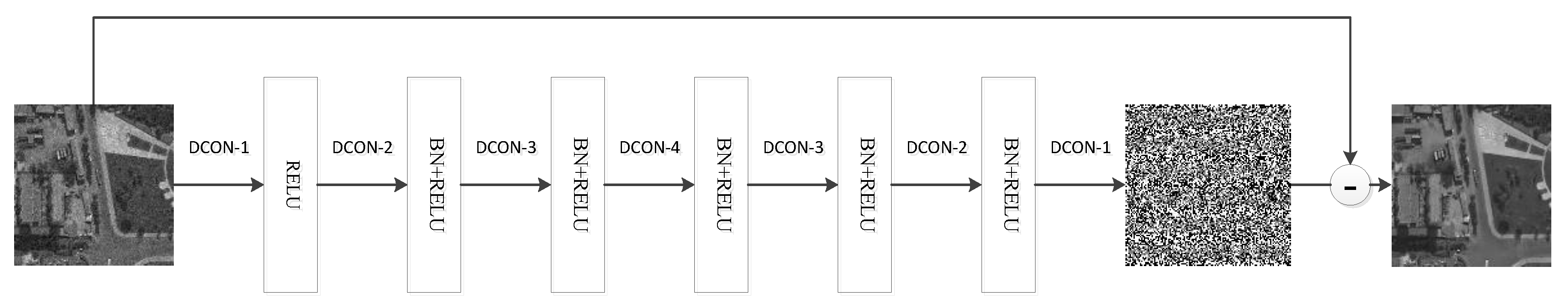
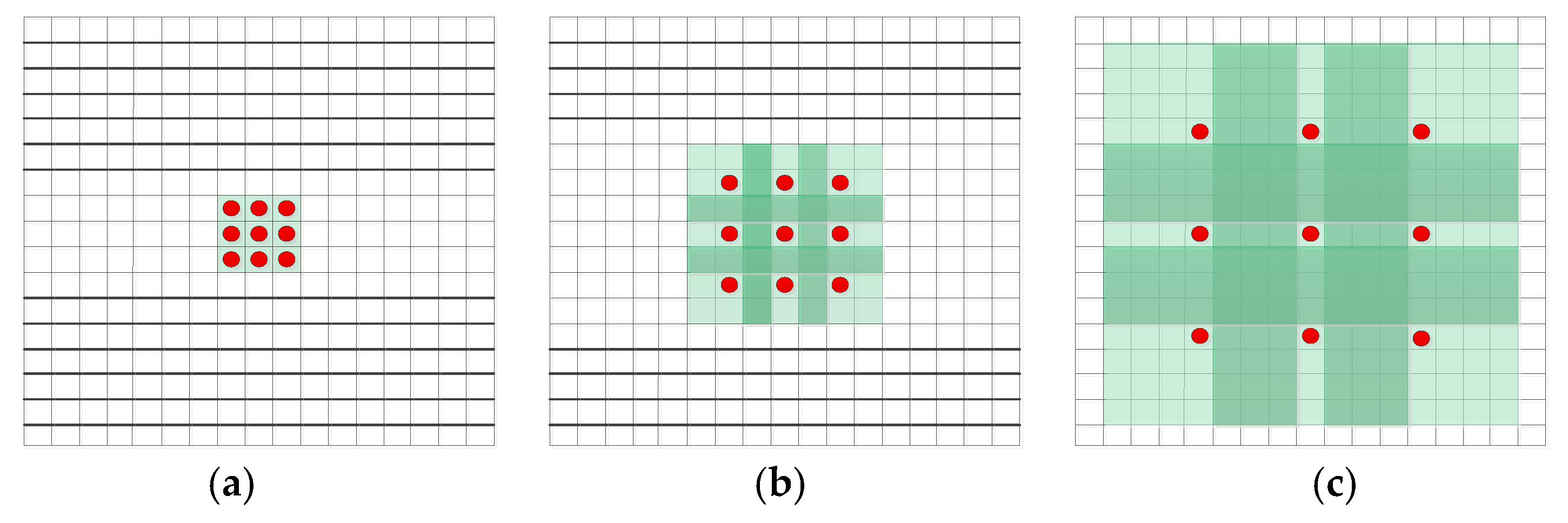
The architecture of CNN in this paper is the same as that in [12], as shown in Figure 1. It has three different modules consisting of a seven-layer network. In Figure 1, “DCon-s” indicate dilated convolutions, and s = 1, 2, 3, and 4, “BN” denotes batch normalization, and “ReLU” represents rectified linear units. The first layer is “Dilated Convolution + ReLU”, and the dilated convolution operation is as follows: Each parameter in the convolution kernel expands according to the inflation factor in the four directions of up, down, left, and right. The number of convolution kernel parameters does not change, and the receptive field becomes large. An example for dilated convolution is given in Figure 2. Figure 2a is a normal convolution. After 1-dilated convolution, we can get a receptive field of . Figure 2b is obtained from Figure 2a through 2-dilated convolution, and we can get a receptive field of . Figure 2c is obtained from Figure 2b through 4-dilated convolution, we can get a receptive filed of . The middle layers have five blocks. Each block represents “Dilated Convolution + Batch Normalization + ReLU”, and the last layer is a “Dilated Convolution” block. We set the expansion factors of the dilated convolution as 1, 2, 3, 4, 3, 2, and 1 from the front to back. The number of feature maps was set to 64 for each middle layer. Next, the important details of the network design and training are illustrated.
Firstly, the network model uses the dilated convolution to balance the size of the receptive field and the depth of the network. We know about the dilated convolution because of its expansion ability in the receptive field while retaining the advantages of a traditional convolution. An expansion filter with an expansion factor s can be simply translated to a sparse filter, where only nine fixed position terms can be non-zero. Therefore, 3, 5, 7, 9, 7, 5, and 3 are the equivalent receptive domains for each layer, respectively. We know that the size of the receptive field is .
Secondly, residual learning and batch normalization are used for the network model to speed up the training. They are two of the most influential architecture design techniques in CNN network structure design. The combination of these two techniques means that the CNN does not have immediate stabilizing training, but it can more easily produce a better denoising performance [12].
Thirdly, the network model uses small size training samples to prevent boundary artifacts. Owing to the characteristics of convolution operations, image boundary processing may result in boundary artifacts when denoised images of CNN are not properly processed. Zhang et al. [12] found that using the zero padding boundary expansion strategy by utilizing a small training sample size helps to prevent boundary artifacts, since the small blocks allow the CNN to use more boundary information. Therefore, an image block is cropped into small non-overlapping blocks in the network model to strengthen the boundary information of the image.
For training the CNN, we used a dataset consisting of 400 Berkeley segmentation dataset images of size 180 × 180, as mentioned in [12]. For convenience, we converted the images to gray images, and we cropped the images into small patches of size 35 × 35 and selected 12,000 patches for training. As for the generation of corresponding noisy patches, we achieved this by adding additive Gaussian noise to the clean patches during training. During training, the loss function of CNN was the same as the loss function in [12].
Finally, the network model trains specific denoisers with small spaced noise levels for noise images with different noise levels. Ideally, the denoisers in Equation (9) should use the training set of the current noise level to train the network model. Zhang et al. [12] trained a series of denoisers with a noise level range of [0, 50] and divided it by a step size of 2 for each model, resulting in a total of 25 denoisers. Since the small fluctuation of the SAR image noise level have less effect on the denoising result, we chose CNN denoisers with noise levels of 5, 10, 15, 20, and 25 to remove the speckle and then fused the five denoised images to obtain the final denoised image. The GFF algorithm employed in this paper is briefly introduced below.
3. Image Fusion-Based Guided Filtering
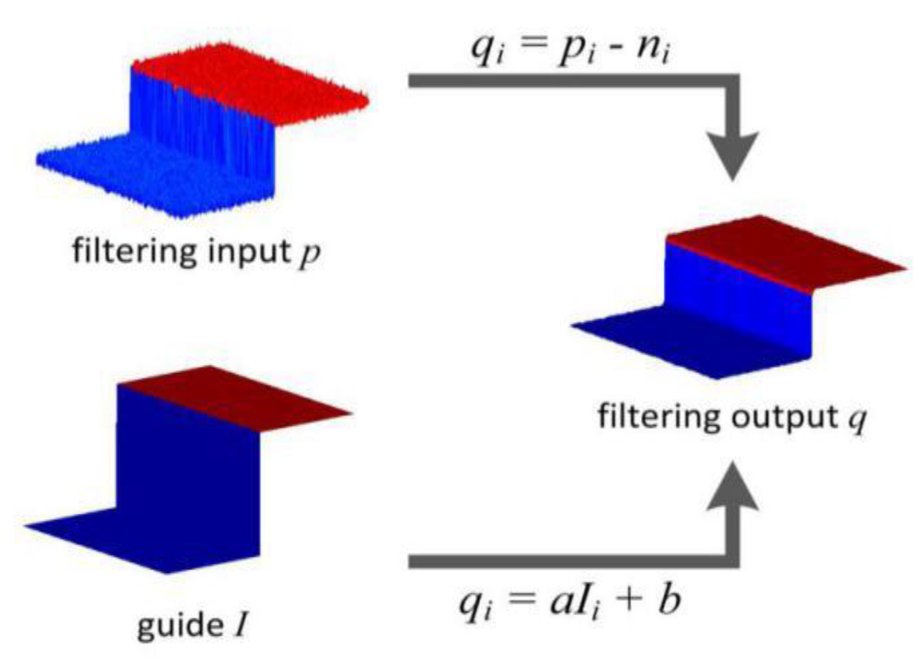
Derived from a local linear model, the guided filter computes the filtering output by considering the content of a guidance image, which can be the input image itself or another different image. The guided filter can be used as an edge-preserving smoothing operator, like the popular bilateral filter, but it has better behavior near the edges. The guided filter is also a more generic concept beyond smoothing: it can transfer the structures of the guidance image to the filtering output. Moreover, the guided filter naturally has a fast and non-approximate linear time algorithm, regardless of the kernel size and the intensity range. Thus, guided filtering is applied widely to the image processing field [37]. We suppose that the guided image is , the input image is (i.e., the image needs to be filtered), and the output image is . The local linear model is the vital assumption of guided filtering between the guided image and the output image, that is,
where are the linear coefficients, is a pixel index, and is the local window centered on the point in the guided image . It is a square window whose size is .
The edge-preserving filtering problem of the image is transformed into an optimization problem. The optimization problem involves minimizing the difference between and when meeting the linear relationship in Equation (11). That is, we should solve the minimization optimization problem, Equation (12):
where is the normalization factor. We can use linear regression [37] to solve Equation (12):
where and represent the mean and variance of the local window in . represents the number of pixels in the window, and the mean of p in the window is . To ensure the calculation amount of in Equation (11) does not change with the change of the local window, we apply mean filtering to and in the local window after calculating and . For simplicity, we adopt to represent guided filtering, where is the size of the filtering kernel, and is the normalization factor. Figure 3 gives an example to show the guided filtering process when and .
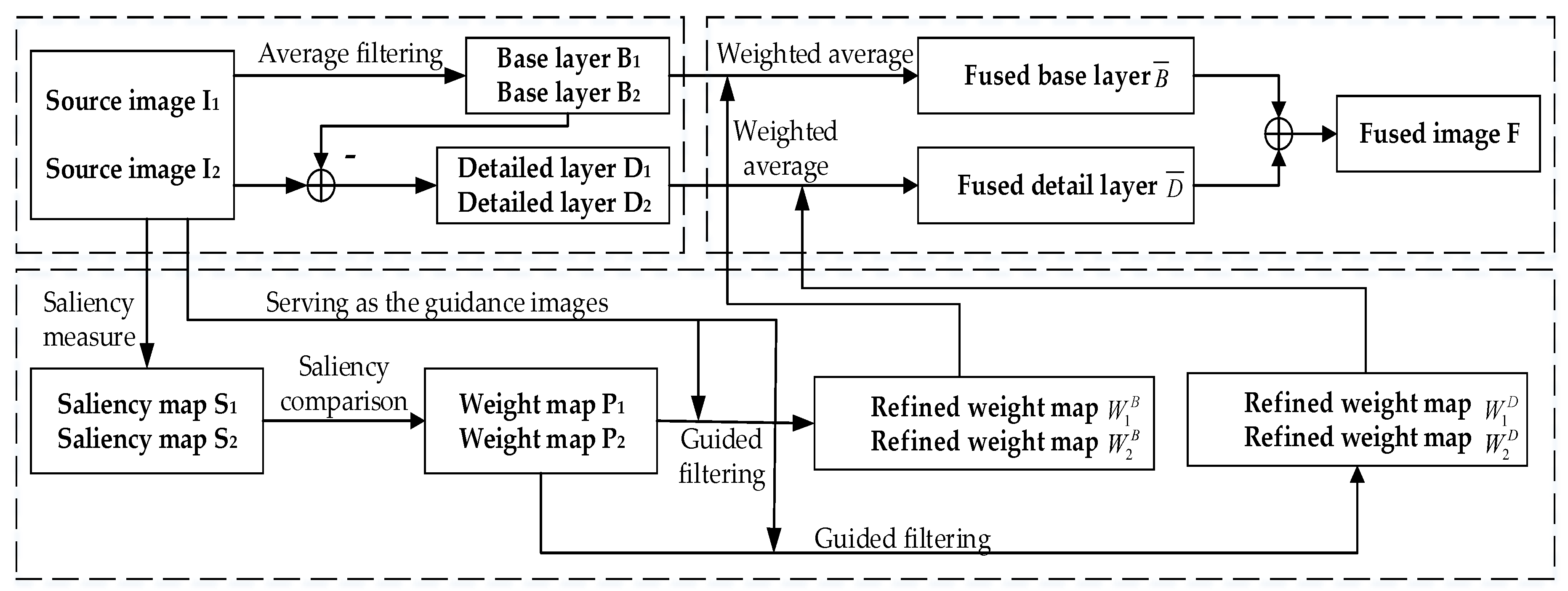
An image fusion algorithm with guided filtering is given in Figure 2 [30]. First of all, the source image is decomposed into two scales by mean filtering, namely the basic layer and the detailed layer . Then, we apply Laplacian filtering to obtain the high-pass portion for each source image . The saliency map is constructed through the local averages of the absolute values of . We use a large saliency map in the source image to construct the weight map . Next, we use the corresponding source image as a guide image for performing guided filtering on each weight map . We get
where , , and are the parameters of the filter, and and are the final weight maps of the basic layer and the detailed layer.
Then, the basic layers and the detailed layers of different original images are merged by the weighted average:
Finally, the fused image is acquired by .
In GFF, the size of should be decided experimentally. To fuse the base layers, the size of is . A big filter size is preferred. To fuse the detailed layers, the size of is , and the fusion performance will be worse when the filter size is too big or too small. In this paper, the value of was set to 45 and the value of was set to 7 based on the experiment. The flow diagram of GFF is shown in Figure 4.
4. CNN Denoiser Prior and Guided Filtering for SAR Image Denoising
In the SAR image, the relative phase between the scattering points in each resolution unit is closely related to the radar azimuth. The speckle is considered to be produced by the coherent superposition of the echoes of many scattering points, which randomly distribute in the same resolution of the scene. It has been proven that fully developed speckle is multiplicative noise by Goodman [9], and its multiplicative model is as follows:
where denotes the SAR image contaminated by speckle; indicates the radar scattering characteristic of the ground target (i.e., the clear image); and denotes the speckle due to fading. The random process and are independent. conforms to a Gamma distribution where the mean is one and the variance is :
where , , is the Gamma function, and is the equivalent number of looks (ENL).
The main purpose of denoising is to eliminate and to restore from . To facilitate the denoising process, homomorphic filtering is usually chosen in Equation (17), and the multiplication model is replaced by an addition model, as shown in Equation (19):
It can be seen that the current noise can be assumed to obey a Gaussian distribution [38]. Thus, Equation (19) can be rewritten as , where represents the observed image, is the additive noise, and is the clean image. Therefore, the SAR image can be denoised by the above denoising algorithm.
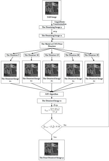
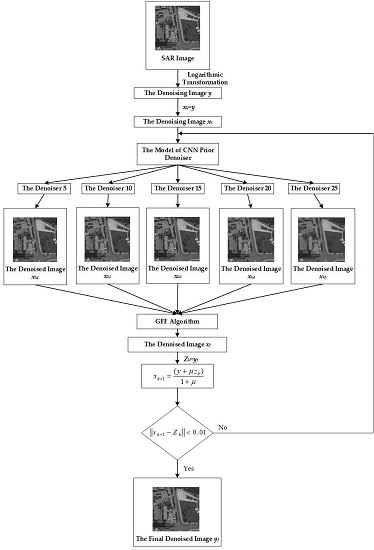
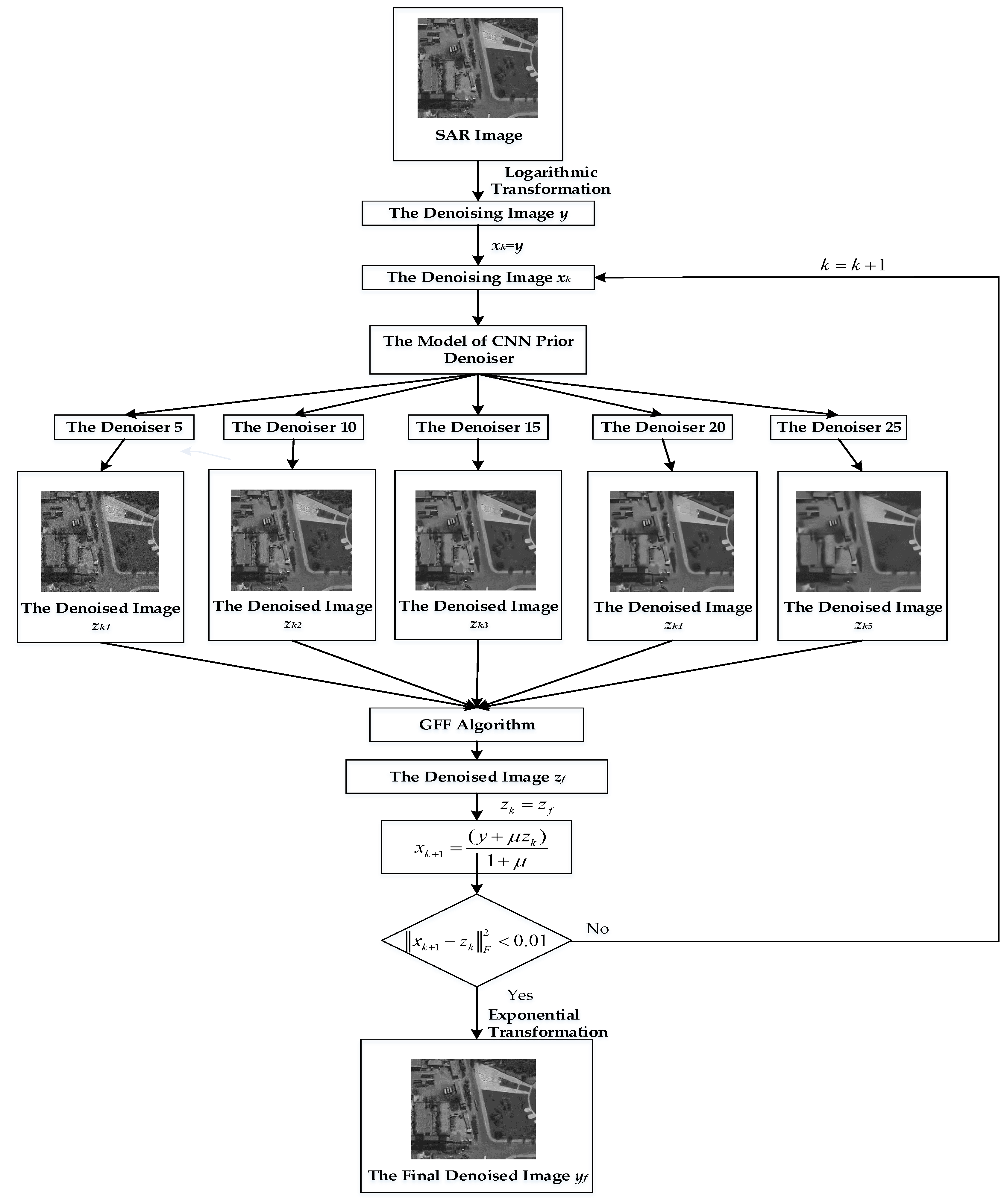
Figure 5 gives the flow chart of SAR image denoising based on CNN denoiser priors and the guided filtering fusion algorithm.
The specific algorithm workflow of this paper is as follows:
Step 1: Equation (19) is used to process the original SAR image by homomorphic filtering and to obtain the denoising image called ;
Step 2: Train the CNN prior denoisers;
Step 3: The initial value of is ;
Step 4: The CNN denoisers are adopted with noise levels of 5, 10, 15, 20, and 25 to denoise the image and to get the denoised images , , , , and by Equation (10);
Step 5: The denoised images , , , , and are fused to obtain the denoised image by the GFF fusion algorithm with Equations (15) and (16). Here, five images are fused instead of two images through the process in Figure 3;
Step 6: Assign the value of to . From Equation (8), we can get ;
Step 7: Let , and repeat Step 4, Step 5, and Step 6 until the norm of and is less than 0.01;
Step 8: The image is indexed to obtain the final denoised image .
5. Experimental Results
The training sets and training process of the CNN denoisers used in this paper are the same as those described in the literature [12]. The denoiser model training platform used was Matlab R2014b which is from Mathworks company in Natick, MA, USA, the CNN toolbox was MatConvnet (MatConvnet-1.0-beta24, Mathworks, Natick, Massachusetts, USA), and the GPU platform was Nvidia Titan X Quadro K6000 (Santa Clara, California, USA) which is from NVIDIA Corporation in Santa Clara, CA, USA. The parameters of the GFF algorithm used in our algorithm were the same as those described in the literature [30].
In order to verify the reliability and effectiveness of the proposed algorithm, the proposed algorithm was tested on a simulated SAR image. The specific steps of the experiment were as follows:
The first step was to convert the clean SAR image into the logarithmic domain to obtain the logarithmic SAR image by using the logarithmic function.
In the second step, a random matrix whose size is the same as the logarithmic SAR image is produced according to various noise variance, the noise variance that this paper is based on is 0.04, 0.05, 0.06, respectively. Then, add the random matrix, which is Gaussian noise to the logarithmic SAR image. Finally, the simulated noise SAR images are obtained.
In the third step, with the simulated noise SAR image as input, the proposed algorithm was used to obtain the denoised image.
In the fourth step, the denoised image was exponentially transformed to obtain the final denoised image.
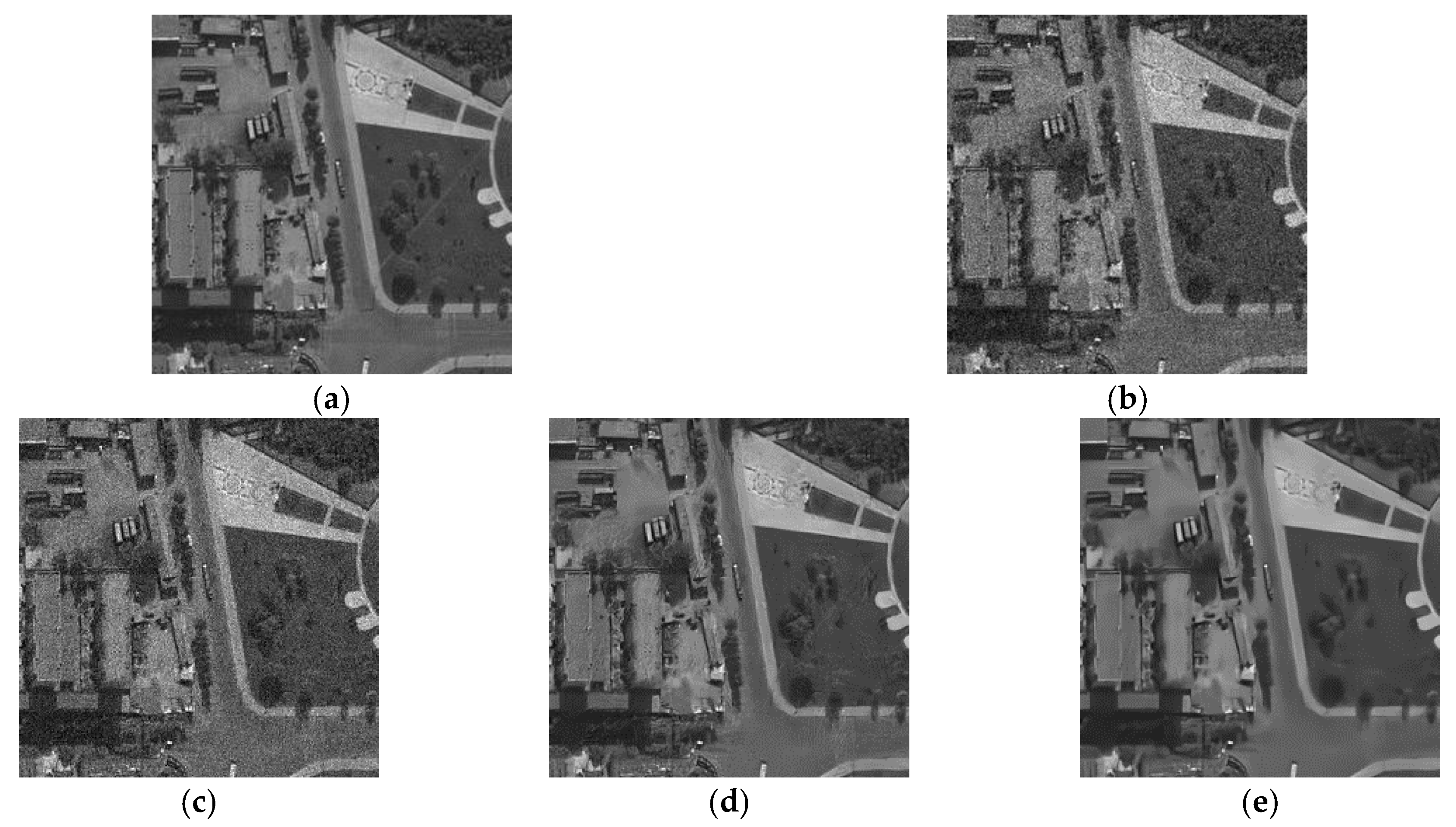
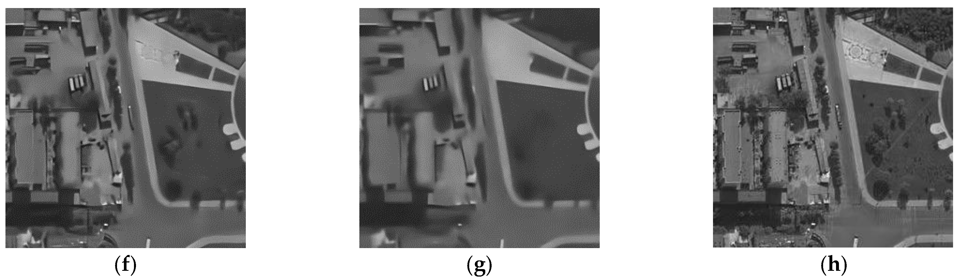
Figure 6a,b show the original image and the noise image, respectively, the six images in (c), (d), (e), (f), (g), and (h) are the denoised images produced through denoisers whose noise levels were 5, 10, 15, 20, and 25, and the final denoised image was produced by using the proposed method. Figure 6c indicates that, when the selected denoiser level is smaller than the ground truth noise level, the denoised image still has a lot of noise, while (f) and (g) illustrate that, when the selected denoiser level is bigger than the ground truth noise level, the denoised image will appear to be over-smoothed. Thus, we fused all the denoised images using the GFF algorithm in order to obtain better denoised results, as shown in Figure 6h. It turned out that the denoised image obtained by the proposed algorithm had less noise while retaining the detailed texture and having a promising visual effect.
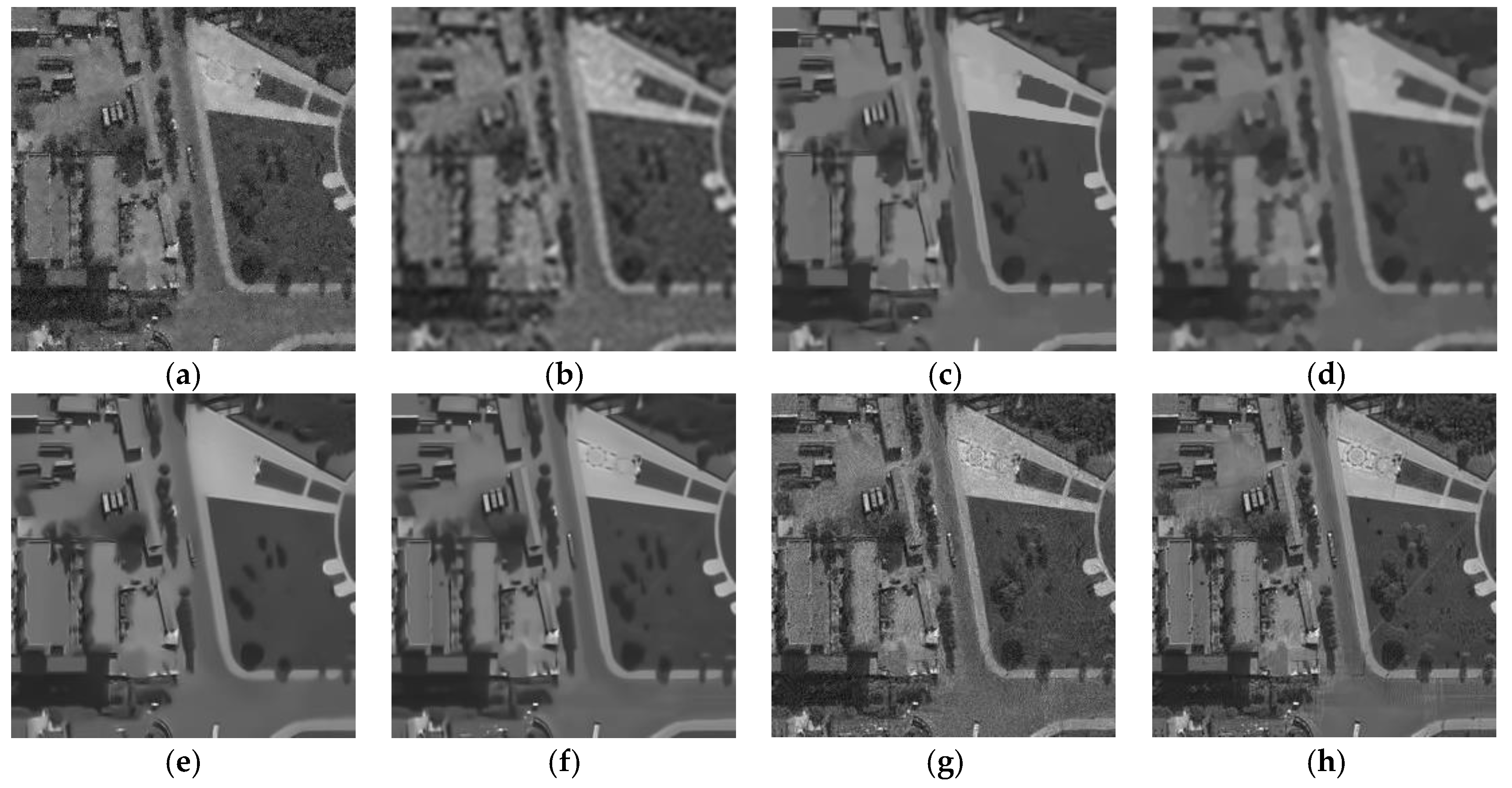
Figure 7 shows a comparison between the proposed algorithm and other denoising algorithms. For all algorithms, the images in the figure had added Gaussian noise with 0.05 noise variance. The denoising algorithms used were the Lee filter [1]; the sparse representation-based Bayesian threshold shrinkage denoising algorithm in the Shearlet domain (BSS-SR), as described in [39]; the local linear minimum-mean-square-error (LLMMSE) wavelet shrinkage-based nonlocal denoising algorithm for SAR image (SAR-BM3D), as described in [40]; SAR image denoising based on continuous cycle spinning via sparse representation in the Shearlet domain (CS-BSR), as described in [41]; probabilistic patch-based weights iteration weighted maximum likelihood denoising (PPB), as described in [42]; the use of texture strength and weighted nuclear norm minimization for SAR image denoising (BWNNM), as described in [43]; deep CNN based on residual learning for image denoising (DnCNN), as described in [44]; and the proposed algorithm.
By observing the experimental results, we found that Figure 7a still retains much noise after Lee filtering, and the edge of the denoised images shown in Figure 7b,d have some blur after the BSS-SR and CS-BSR methods. Although the SAR-BM3D and the PPB methods effectively suppress the speckle, they lose a lot of detail and appear to be over-smoothed, as shown in Figure 7c,e. The BWNNM method and DnCNN algorithm have a good noise suppression effect and better preserve the edge, but there is still some residual noise, as shown in Figure 7f,g. The proposed algorithm, as shown in Figure 7h, achieves a better visual effect than BWNNM and SAR-BM3D, and the noise is more effectively suppressed than with BSS-SR and CS-BSR. These experimental results demonstrate the advantages of the denoising algorithm based on convolutional neural networks and guided filtering.
To further validate the advantages of the algorithm in this thesis, we used five objective evaluation indexes to evaluate the above denoised algorithms: the peak signal to noise ratio (PSNR) [45], the equivalent number of looks (ENL) [45], the edge preservation index (EPI) [14], the structural similarity index measurement (SSIM), and an unassisted measure of the quality of the first-order and second-order descriptors of the denoised image ratio (UM) [14]. The higher the PSNR value is, the stronger the denoising ability of the algorithm is. If the ENL value is bigger, the visual effect is better. The EPI value reflects the retentive ability of the boundary, and a bigger value is better. The SSIM indicates the similarity of the image structure after denoising, and it is as big as possible. The UM does not depend on the source image to assess the denoised image—when the value is smaller, the ability of the speckle suppression is stronger. The evaluation parameter values of the denoised images are given in Table 1.
We can obtain from Table 1 that the PSNR value of all the algorithms improved compared to that of the original image when noise with variance of 0.04 was added to images. Obviously, all algorithms can effectively suppress speckle, but our method had the highest PSNR value. The ENL value of the proposed algorithm improved compared with that of DnCNN, which indicates the effectiveness of the fusion algorithm based on guided filtering. Because of the complex and inherent denoising structure of CNN, it had a worse ENL value than the other algorithms. The results of our method in terms of retaining image edge information and texture detail are satisfying. The ENL value was higher than most of the other algorithms by about 0.1 to 0.2, and it was higher than the Lee filter by about 0.4. At the same time, the SSIM results show that the proposed method maintains the integrity of the image structure and has minimum structural distortion.
Meanwhile, our method also achieved the best results on the three evaluation indexes of PSNR, EPI and SSIM when noise with variance of 0.05 was added to images. Through Table 1, we can see that the SSIM of BSS-SR, SAR-BM3D, and other algorithms decreased slightly, which means that these algorithms cannot retain the detail and reduce the distortion simultaneously, but our method, as well as the DnCNN and Lee filter, showed satisfactory results. Moreover, the ENL value of our method remained stable, which is better than that of DnCNN. When we added noise with variance of 0.06 to the image, the experimental results were the same as those analyzed above.
Generally speaking, whatever the noise level is, our proposed algorithm can preserve the structural information of the image, suppress the noise effectively, and retain the edge details to some extent.
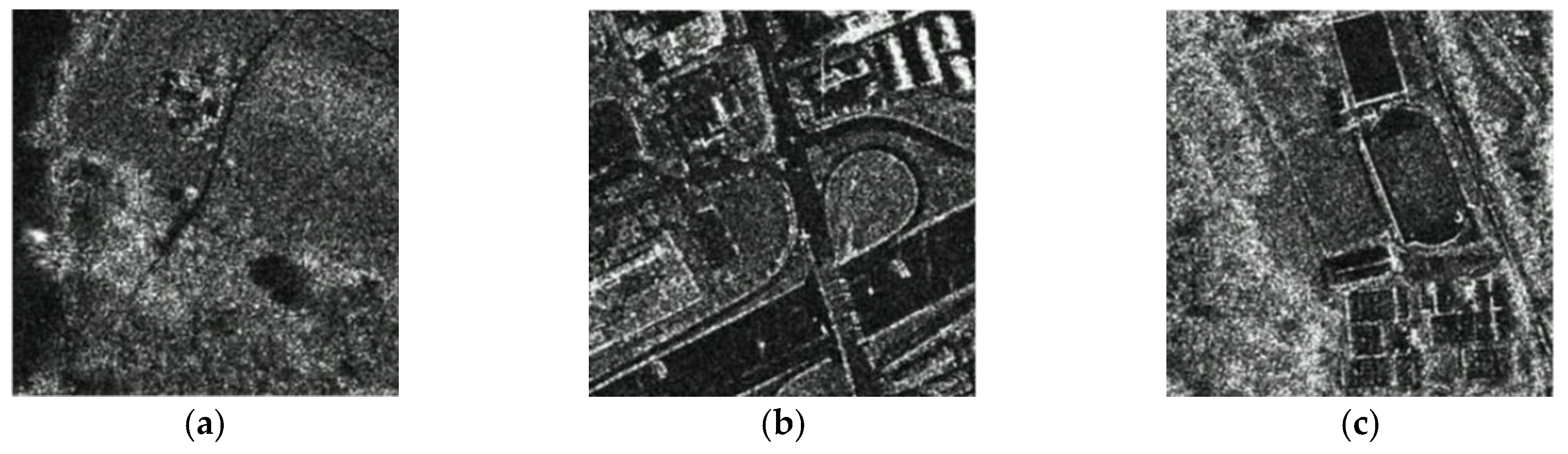
Moreover, our proposed algorithm was tested by using the actual SAR image. The test images were the SAR images of TerraSar-X, and they can be downloaded from the website of Federico II University in Naples, Italy. They are shown in Figure 8.
Figure 8a shows an SAR image of trees, Figure 8b shows an SAR image of a city area, and Figure 8c shows an SAR image of a lake. They were denoised by the above denoising algorithms.
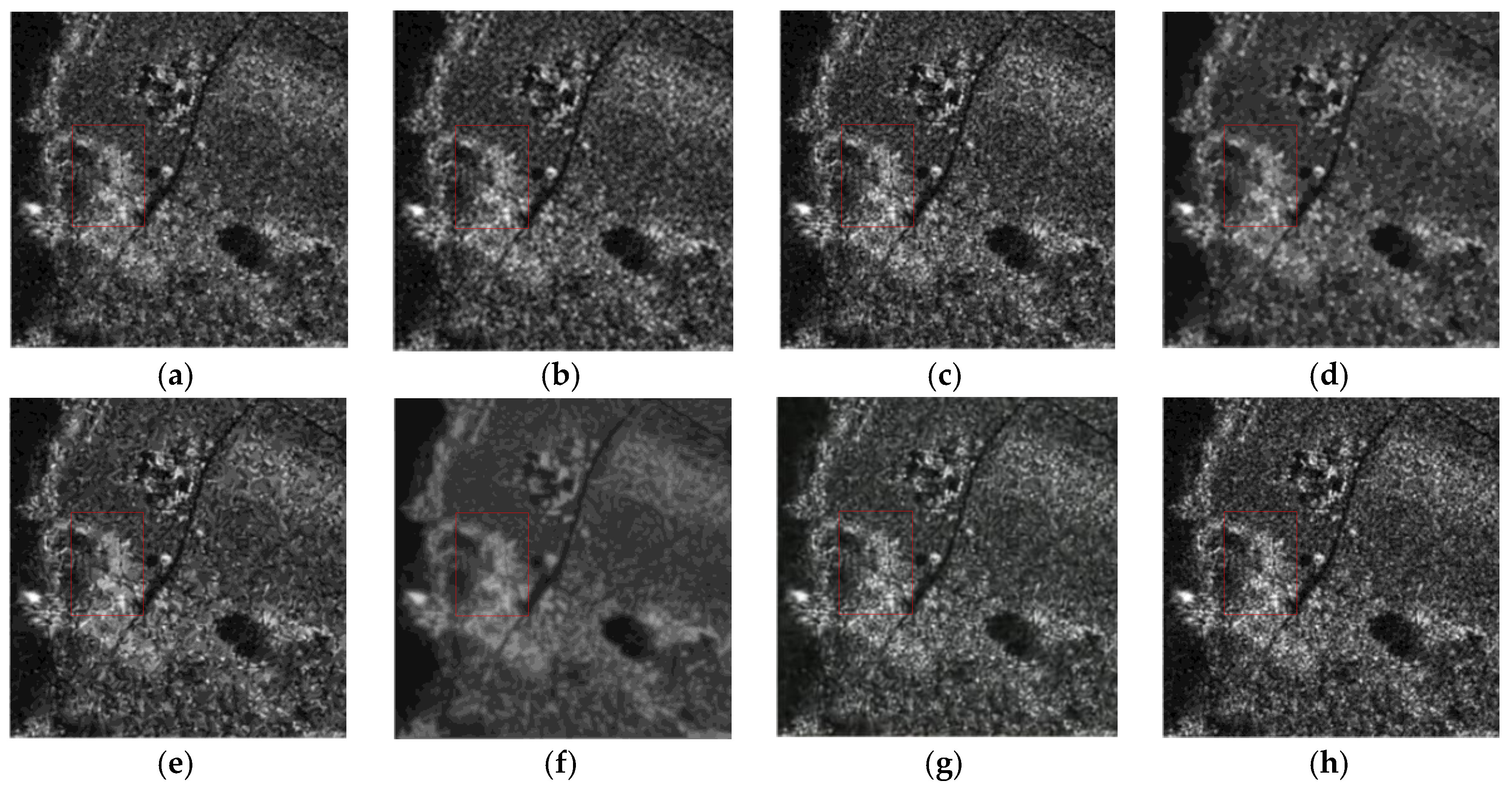
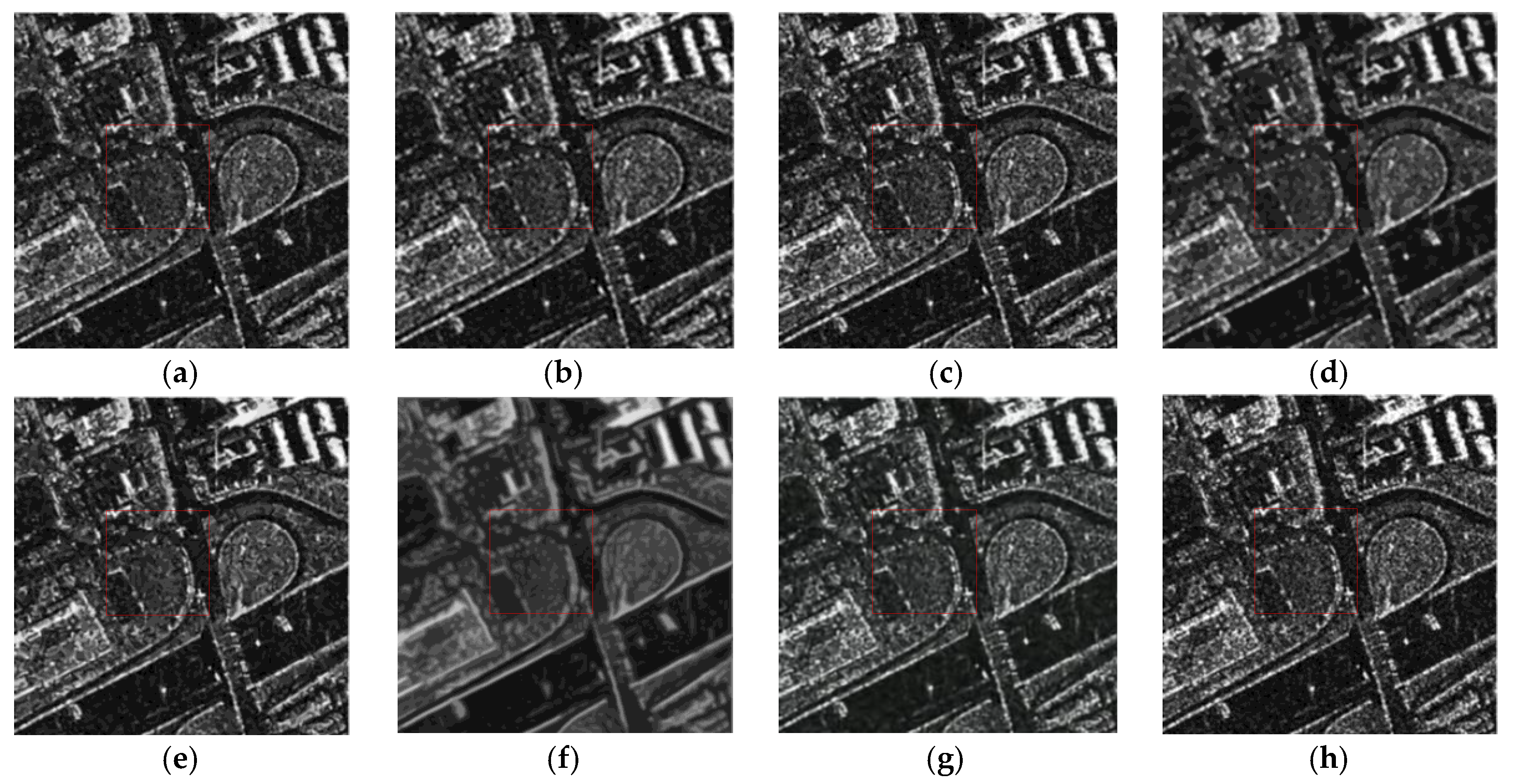
Figure 9 shows the denoised images of Figure 8a. In addition, the red boxes in Figure 9, Figure 10 and Figure 11 mark out the region of the objective evaluation parameter UM. The specific values are given in the objective evaluation index section. We can see that the Lee filter is the worst denoising algorithm from Figure 9. BSS-SR and CS-BSR blurred some edge texture, while SAR-BM3D and PPB brought in little artificial texture. BWNNM and DnCNN produced over-smoothing. Our algorithm not only preserved the texture and edge information well, but it also suppressed the generation of artificial texture.
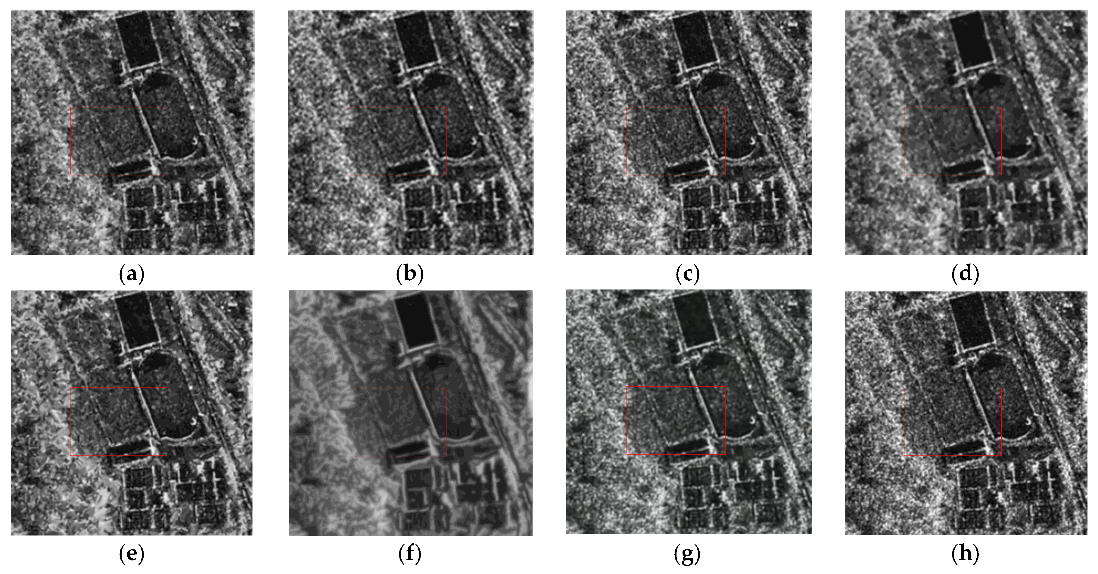
Figure 10 shows the denoised images of the city area in Figure 8b by using different denoising algorithms, and Figure 11 shows the denoised images of a lake SAR in Figure 8c by using different denoising algorithms.
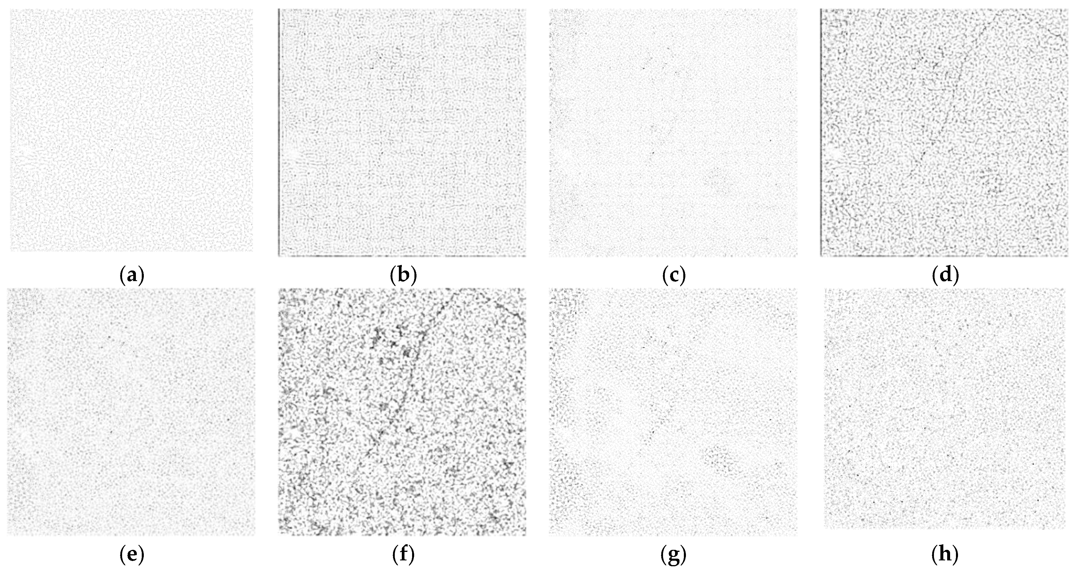
As shown in Figure 10 and Figure 11, the performances of the eight denoising algorithms presented in this paper are similar to the results shown in Figure 8a. The denoising effect of our proposed algorithms is the most promising. However, we have neither the clean image nor an expert interpreter, which is difficult to ensure whether such artifacts mean any loss of detail. Some help comes from the analysis of ratio images obtained, as mentioned in [40], as the pointwise ratio between the original SAR image and de-noised SAR images. Given a perfect denoising, the ratio image should only contain speckle. On the contrary, the existence of structures or details related to the original image shows that the algorithm has removed not only noise but also some useful information. In order to highlight the better visual effect of our method, we give the ratio images in Figure 12, Figure 13 and Figure 14.
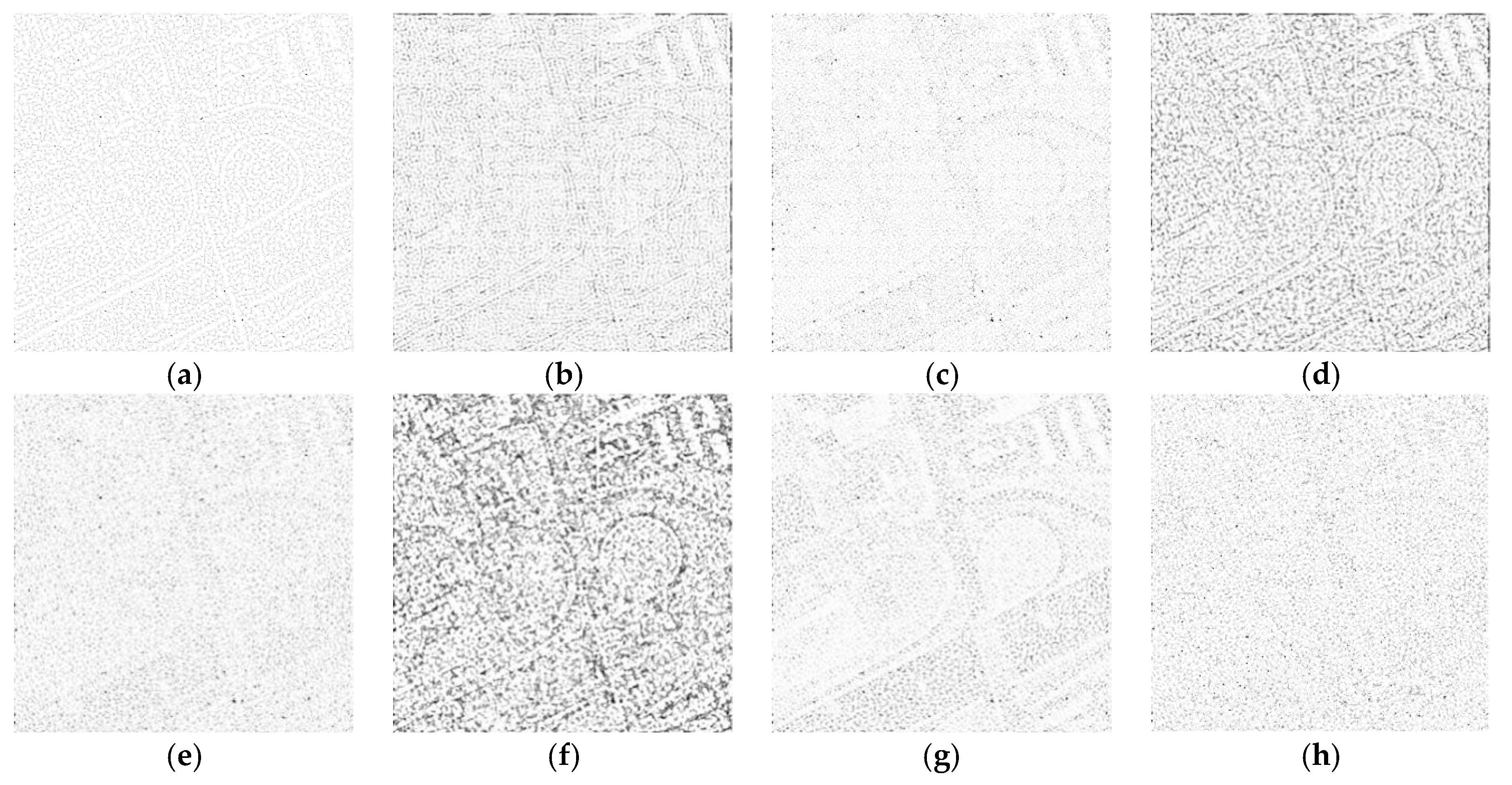
From Figure 12, we can see that the ratio image of our algorithm is closer to speckle. Figure 13 gives the ratio images from Figure 10.
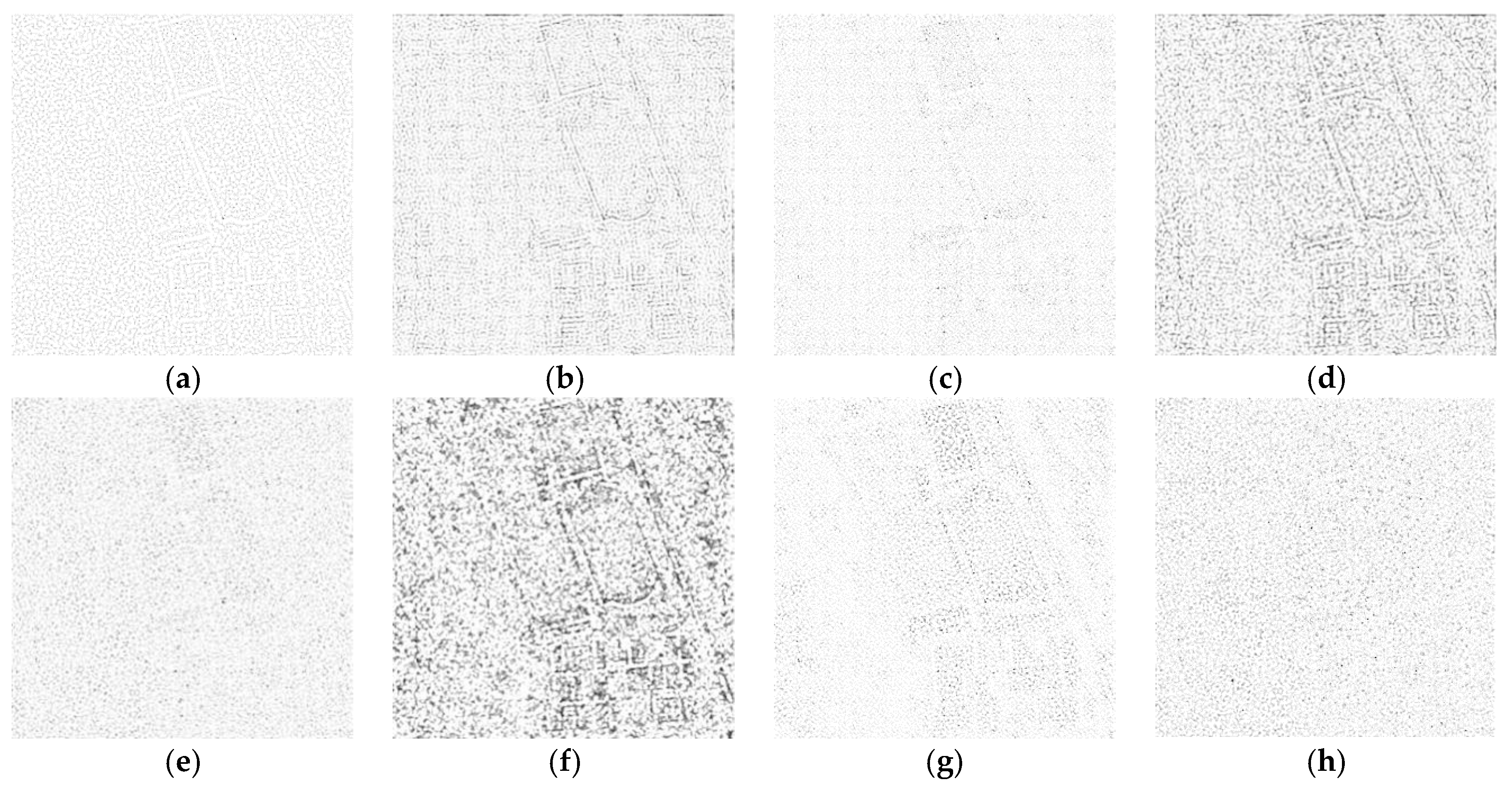
From the ratio images in Figure 12, Figure 13 and Figure 14, we can find that our method have no obvious pattern and obtain the least signal information. From this view, it can show that our method can attain a better visual effect.
To show the superiority of our algorithm, we used various common objective evaluation parameters for the denoising algorithms, including UM, ENL, EPI and SSIM. Table 2, Table 3 and Table 4 give the experimental results of the objective evaluation results of the above denoised images.
Table 2 presents the results of evaluation indexes of the tree SAR image denoised by eight algorithms. First of all, the UM value was 25.4 of our proposed algorithm, and it was the smallest and the best of the eight algorithms. This shows that the proposed algorithm has an excellent comprehensive performance in terms of noise suppression. The ENL value of our method was not ideal, but its value was still bigger than the DnCNNs. The reason for this phenomenon is not only the complex and inherent denoising structure of CNN, but it is also related to the texture, light, and shade of SAR images. Finally, it is easy to see that the EPI and SSIM values of our method were the biggest, which shows that our proposed method has the strongest ability to preserve edges, and the integrity of the image structure was also the best.
As shown in Table 3 and Table 4, the performances of all the algorithms basically showed a similar trend to those in Table 2. Compared with other methods, we found that our method significantly improved UM, EPI, and SSIM. In summary, our algorithm possesses the best denoising ability, the strongest edge and detail preservation ability, and the most promising visual effects.
Without any loss of generality, the abilities to preserve detailed information and smoothness are contradictory in our method. Although our method is better than the Lee filter for ENL, it is not as good as PPB or SAR-BM3D because the selection of the CNN model and fusion algorithm is just empirical. If there were more suitable models and fusion methods, the performance of our method could be improved furtherly.
6. Conclusions
In this paper, a novel SAR image denoising algorithm based on CNN and the guided filtering fusion algorithm was proposed. First, five different noise level denoisers from the prior set of CNN denoisers were used to obtain five denoised SAR images. Then, the five denoised images were fused with guided filtering to obtain the final denoised image. The experimental results indicate that our proposed algorithm can significantly increase the PSNR after image denoising, effectively suppress the speckle noise, maintain the edge and detail information, and obtain promising visual effects. However, due to the limitation of the CNN structure, our proposed algorithm cannot obtain the highest ENL and EPI values at the same time, which could be a future task for this field.
Author Contributions
S.L. proposed the method; S.L. and T.L. designed and performed the experiments; S.L., T.L., Q.H. and H.L. wrote the manuscript and modified the paper; L.G. did the data validation; J.Z. and C.W. supervised the process. All the authors read and testified the final results.
Funding
This research was funded by the Natural Science Foundation of China under Grant Nos. 61401308 and 61572063, the Natural Science Foundation of Hebei Province under Grant No. F2016201142, F2016201187 and F2018210148, the Science research project of Hebei Province under Grant No. QN2016085, the Natural Science Foundation of Hebei University under Grant No. 2014-303, the Opening Foundation of Machine vision Engineering Research Center of Hebei Province under Grant No. 2018HBMV02, and the Post-graduate's Innovation Fund Project of Hebei University under Grant No. hbu2018ss01.
Acknowledgments
This work is supported by the High-Performance Computing Center of Hebei University.
Conflicts of Interest
The authors declare no conflict of interest.
References
- Lee, J.S. Refined filtering of image noise using local statistics. Comput. Graph. Image Process. 1981, 15, 380–389. [Google Scholar] [CrossRef] [Green Version]
- Akl, A.; Tabbara, K.; Yaacoub, C. An enhanced Kuan filter for suboptimal speckle reduction. In Proceedings of the International Conference on Advances in Computational TOOLS for Engineering Applications, Beirut, Lebanon, 12–15 December 2012; pp. 91–95. [Google Scholar]
- Lopes, A.; Touzi, R.; Nezry, E. Adaptive speckle filters and scene heterogeneity. IEEE Trans. Geosci. Remote Sens. 1990, 28, 992–1000. [Google Scholar] [CrossRef]
- Gagnon, L.; Jouan, A. Speckle filtering of SAR images: A comparative study between complex-wavelet-based and standard filters. In Proceedings of the SPIE Meeting: Wavelet Applications in Signal and Image Processing, San Diego, CA, USA, August 1997; pp. 80–91. [Google Scholar]
- Chen, S.; Gao, L.; Li, Q. SAR image despeckling by using nonlocal sparse coding model. Circuits Syst. Signal Process. 2017, 37, 1–23. [Google Scholar] [CrossRef]
- Min, D.; Cheng, P.; Chan, A.K.; Loguinov, D. Bayesian wavelet shrinkage with edge detection for SAR image despeckling. IEEE Trans. Geosci. Remote Sens. 2004, 42, 1642–1648. [Google Scholar] [CrossRef] [Green Version]
- Fang, J.; Wang, D.; Xiao, Y.; Ajay Saikrishna, D. De-noising of SAR images based on Wavelet-Contourlet domain and PCA. In Proceedings of the International Conference on Signal Processing, Hangzhou, China, 19–23 October 2014; pp. 942–945. [Google Scholar]
- Puranikmath, S.S.; Kaliyaperumal, V. Enhancement of SAR images using curvelet with controlled shrinking technique. Remote Sens. Lett. 2016, 7, 21–30. [Google Scholar]
- Rezaei, H.; Karami, A. SAR image denoising using homomorphic and shearlet transforms. In Proceedings of the International Conference on Pattern Recognition & Image Analysis, Shahrekord, Iran, 19–20 April 2017; pp. 1–5. [Google Scholar]
- Liu, S.; Shi, M.; Hu, S.; Yang, X. Synthetic aperture radar image de-noising based on Shearlet transform using the context-based model. Phys. Commun. 2014, 13, 221–229. [Google Scholar] [CrossRef]
- Liu, S.; Zhang, Y.; Hu, Q.; Liu, M.; Zhao, J. SAR image de-noising based on GNL-means with optimized pixel-wise weighting in non-subsample shearlet domain. Comput. Inform. Sci. 2017, 10, 16–22. [Google Scholar] [CrossRef]
- Zhang, K.; Zuo, W.M.; Gu, S.H.; Zhang, L. Learning deep cnn denoiser prior for image restoration. In Proceedings of the IEEE Conference on Computer Vision and Pattern Recognition(CVPR), Honolulu, HI, USA, July 2017; pp. 2808–2817. [Google Scholar]
- Lu, T.; Li, S.; Fang, L.; Benediktsson, J.-A. SAR image despeckling via structural sparse representation. Sens. Imaging 2016, 17, 1–20. [Google Scholar] [CrossRef]
- Liu, S.; Hu, Q.; Li, P.; Zhao, J.; Zhu, Z. SAR image denoising based on patch ordering in nonsubsample shearlet domain. Turk. J. Electr. Eng. Comput. Sci. 2018, 26, 1860–1870. [Google Scholar] [CrossRef]
- Deledalle, C.A.; Denis, L.; Poggi, G.; Tupin, F.; Verdoliva, L. Exploiting patch similarity for SAR image processing: The nonlocal paradigm. IEEE Signal Process. Mag. 2014, 31, 69–78. [Google Scholar] [CrossRef]
- Liu, S.; Hu, Q.; Li, P.; Zhao, J.; Wang, C.; Zhu, Z. Speckle suppression based on sparse representation with non-local priors. Remote Sens. 2018, 10, 439. [Google Scholar] [CrossRef]
- Thapa, D.; Raahemifar, K.; Lakshminarayanan, V. Reduction of speckle noise from optical coherence tomography images using multi-frame weighted nuclear norm minimization method. J. Mod. Opt. 2015, 62, 1856–1864. [Google Scholar] [CrossRef]
- Wu, Y. Speckle noise removal via nonlocal low-rank regularization. J. Vis. Commun. Image Represent. 2016, 39, 172–180. [Google Scholar] [CrossRef]
- Xu, J. Speckle noise filtering algorithm by using wavelet based on PCNN. J. Inform. Comput. Sci. 2013, 10, 2237–2246. [Google Scholar] [CrossRef]
- Huang, X.; Qiao, H.; Zhang, B.; Nie, X. Supervised polarimetric SAR image classification using tensor local discriminant embedding. IEEE Trans. Image Process. 2018, 27, 2966–2979. [Google Scholar] [CrossRef]
- Wang, P.; Zhang, H.; Patel, V.M. SAR image despeckling using a convolutional neural network. IEEE Signal Process. Lett. 2017, 24, 1763–1767. [Google Scholar] [CrossRef]
- Chierchia, G.; Cozzolino, D.; Poggi, G.; Verdoliva, L. SAR image despeckling through convolutional neural networks. IGARSS 2017, 2017, 5438–5441. [Google Scholar]
- Zhang, Q.; Yuan, Q.; Li, J.; Yang, Z.; Ma, X. Learning a dilated residual network for SAR image despeckling. Remote Sens. 2018, 10, 196. [Google Scholar] [CrossRef]
- Hinton, G.; Salakhutdinov, R. Reducing the dimensionality of data with neural networks. Science. 2006, 313, 504–507. [Google Scholar] [CrossRef] [PubMed]
- Qiangqiang, Y.; Qiang, Z.; Jie, L.; Shen, H.; Zhang, L. Hyperspectral Image Denoising Employing a Spatial-Spectral Deep Residual Convolutional Neural Network. IEEE Trans. Geosci. Remote Sens. 2019, 57, 1205–1218. [Google Scholar]
- Wei, Y.; Yuan, Q.; Shen, H.; Zhang, L. Boosting the accuracy of multi-spectral image pan-sharpening by learning a deep residual network. IEEE Geosci. Remote Sens. Lett. 2017, 14, 1795–1799. [Google Scholar] [CrossRef]
- Li, S.; Kang, X.D.; Fang, L.; Hu, J.; Yin, H. Pixel-level image fusion: A survey of the state of the art. Inform. Fusion 2017, 33, 100–112. [Google Scholar] [CrossRef]
- Shen, R.; Cheng, I.; Shi, J.; Basu, A. Generalized random walks for fusion of multi-exposure images. IEEE Trans. Image Process. 2011, 20, 3634–3646. [Google Scholar] [CrossRef] [PubMed]
- Liu, S.; Shi, M.; Zhu, Z.; Zhao, J. Image fusion based on complex-shearlet domain with guided filtering. Multidimens. Syst. Signal Process. 2017, 28, 207–224. [Google Scholar] [CrossRef]
- Li, S.T.; Kang, X.D.; Hu, J.W. Image fusion with guided filtering. IEEE Trans. Image Process. 2013, 22, 2864–2875. [Google Scholar] [PubMed]
- Gragnaniello, D.; Poggi, G.; Scarpa, G.; Verdoliva, L. SAR image despeckling by soft classification. IEEE J. Sel. Top. Appl. Earth Obs. Remote Sens. 2016, 9, 2118–2130. [Google Scholar] [CrossRef]
- Liu, S.; Liu, M.; Shi, M.Z.; Xin, Q.; Hu, Q. SAR image de-noising based on nuclear norm minimization fusion algorithm. In Proceedings of the International Conference in Communications, Singapore, October 2016; pp. 193–201. [Google Scholar]
- Geman, D.; Yang, C. Nonlinear image recovery with half-quadratic regularization. IEEE Trans. Image Process. 1995, 4, 932–946. [Google Scholar] [CrossRef] [PubMed] [Green Version]
- Bioucas-Dias, J.M.; Figueiredo, M.A. A New TwIST: Two-step iterative shrinkage/thresholding algorithms for image restoration. IEEE Trans. Image Process. 2007, 16, 2992–3004. [Google Scholar] [CrossRef] [PubMed]
- Ciccone, V.; Ferrante, A.; Zorzi, M. Factor models with real data: A robust estimation of the number of factors. IEEE Trans. Autom. Control 2018, 1–13. [Google Scholar] [CrossRef]
- Liégeois, R.; Mishra, B.; Zorzi, M.; Sepulchre, R. Sparse plus low-rank autoregressive identification in neuroimaging time series. In Proceedings of the 54th IEEE Conference on Decision and Control, Osaka, Japan, 15–18 December 2015; pp. 3965–3970. [Google Scholar]
- He, K.; Sun, J.; Tang, X. Guided image filtering. IEEE Trans. Patt. Anal. Mach. Intel. 2013, 35, 1397–1409. [Google Scholar] [CrossRef] [PubMed]
- Xue, B.; Huang, Y.; Yang, J.; Shi, L.; Zhan, Y.; Cao, X. Fast nonlocal remote sensing image denoising using cosine integral images. IEEE Geosci. Remote Sens. Lett. 2013, 10, 1309–1313. [Google Scholar] [CrossRef]
- Liu, S.Q.; Hu, S.H.; Xiao, Y.; An, Y.L. Bayesian shearlet shrinkage for SAR image de-noising via sparse representation. Multidimens. Syst. Signal Process. 2014, 25, 683–701. [Google Scholar] [CrossRef]
- Parrilli, S.; Poderico, M.; Angelino, C.V.; Verdoliva, L. A nonlocal SAR image denoising algorithm based on LLMMSE wavelet shrinkage. IEEE Trans. Geosci. Remote Sens. 2012, 50, 606–616. [Google Scholar] [CrossRef]
- Liu, S.; Liu, M.; Li, P.; Zhao, J.; Wang, X. SAR image denoising via sparse representation in shearlet domain based on continuous cycle spinning. IEEE Trans. Geosci. Remote Sens. 2017, 55, 2985–2992. [Google Scholar] [CrossRef]
- Deledalle, C.A.; Tupin, F. Iterative weighted maximum likelihood denoising with probabilistic patch-based weights. IEEE Trans. Image Process. 2009, 18, 2661–2672. [Google Scholar] [CrossRef] [PubMed]
- Fang, J.; Liu, S.; Xiao, Y.; Li, H. SAR image de-noising based on texture strength and weighted nuclear norm minimization. J. Syst. Eng. Electron. 2016, 27, 807–814. [Google Scholar]
- Zhang, K.; Zuo, W.; Chen, Y.; Meng, D.; Zhang, L. Beyond a Gaussian denoiser: Residual learning of deep CNN for image denoising. IEEE Trans. Image Process. 2017, 26, 3142–3155. [Google Scholar] [CrossRef] [PubMed]
- Hou, B.; Zhang, X.; Bu, X.; Feng, H. SAR image despeckling based on nonsubsampled shearlet transform. IEEE J. Sel. Top. Appl. Earth Obs. Remote Sens. 2012, 5, 809–823. [Google Scholar] [CrossRef]
Figure 1.
The framework of the denoiser network.

Figure 2.
The example of a dilated convolution process.

Figure 3.
Illustrations of the guided filtering process.

Figure 4.
The flow diagram of the fused algorithm.

Figure 5.
The flow diagram of the proposed algorithm.

Figure 6.
Denoised images using different level denoisers: (a) the source image; (b) the noise image; (c) denoiser 5; (d) denoiser 10; (e) denoiser 15; (f) denoiser 20; (g) denoiser 25; (h) the proposed algorithm.
Figure 6.
Denoised images using different level denoisers: (a) the source image; (b) the noise image; (c) denoiser 5; (d) denoiser 10; (e) denoiser 15; (f) denoiser 20; (g) denoiser 25; (h) the proposed algorithm.


Figure 7.
Denoised images using different methods: (a) Lee filter; (b) BSS-SR; (c) SAR-BM3D; (d) CS-BSR; (e) PPB; (f) BWNNM; (g) DnCNN; (h) our method.
Figure 7.
Denoised images using different methods: (a) Lee filter; (b) BSS-SR; (c) SAR-BM3D; (d) CS-BSR; (e) PPB; (f) BWNNM; (g) DnCNN; (h) our method.

Figure 8.
The real SAR images: (a) trees; (b) city area; (c) lake.

Figure 9.
The denoised tree SAR images using all denoising methods: (a) Lee filter; (b) BSS-SR; (c) SAR-BM3D; (d) CS-BSR; (e) PPB; (f) BWNNM; (g) DnCNN; (h) our method.
Figure 9.
The denoised tree SAR images using all denoising methods: (a) Lee filter; (b) BSS-SR; (c) SAR-BM3D; (d) CS-BSR; (e) PPB; (f) BWNNM; (g) DnCNN; (h) our method.

Figure 10.
The denoised city area SAR images using all denoising methods: (a) Lee filter; (b) BSS-SR; (c) SAR-BM3D; (d) CS-BSR; (e) PPB; (f) BWNNM; (g) DnCNN; (h) our method.
Figure 10.
The denoised city area SAR images using all denoising methods: (a) Lee filter; (b) BSS-SR; (c) SAR-BM3D; (d) CS-BSR; (e) PPB; (f) BWNNM; (g) DnCNN; (h) our method.

Figure 11.
The denoised lake SAR image using all denoising methods: (a) Lee filter; (b) BSS-SR; (c) SAR-BM3D; (d) CS-BSR; (e) PPB; (f) BWNNM; (g) DnCNN; (h) our method.
Figure 11.
The denoised lake SAR image using all denoising methods: (a) Lee filter; (b) BSS-SR; (c) SAR-BM3D; (d) CS-BSR; (e) PPB; (f) BWNNM; (g) DnCNN; (h) our method.

Figure 12.
The ratio images using all denoising methods for Figure 8. (a) ratio image by using lee filter; (b) ratio image by using BSS-SR; (c) ratio image by using SAR-BM3D; (d) ratio image by using CS-BSR; (e) ratio image by using PPB; (f) ratio image by using BWNNM; (g) ratio image by using DnCNN; (h) ratio image by using our method.

Figure 13.
The ratio images using all denoising methods for Figure 9. (a) ratio image by using lee filter; (b) ratio image by using BSS-SR; (c) ratio image by using SAR-BM3D; (d) ratio image by using CS-BSR; (e) ratio image by using PPB; (f) Ratio image by using BWNNM; (g) ratio image by using DnCNN; (h) ratio image by using our method.

Figure 14.
The ratio images using all denoising methods for Figure 10. (a) ratio image using lee filter; (b) ratio image using BSS-SR; (c) ratio image using SAR-BM3D; (d) ratio image using CS-BSR; (e) ratio image using PPB; (f) ratio image using BWNNM; (g) ratio image using DnCNN; (h) ratio image using our method.


Table 1.
The evaluation parameter values of all denoising methods.
| Noise Variance | Denoising Methods | PSNR | ENL | EPI | SSIM |
|---|---|---|---|---|---|
| 0.04 | Lee filter | 32.51 | 6.94 | 0.82 | 0.75 |
| BSS-SR | 31.65 | 7.84 | 0.71 | 0.62 | |
| SAR-BM3D | 33.61 | 8.08 | 0.62 | 0.69 | |
| CS-BSR | 31.48 | 8.92 | 0.63 | 0.58 | |
| PPB | 30.87 | 7.56 | 0.66 | 0.71 | |
| BWNNM | 33.42 | 7.28 | 0.66 | 0.75 | |
| DnCNN | 31.51 | 6.02 | 0.71 | 0.72 | |
| Our method | 38.29 | 6.46 | 0.81 | 0.94 | |
| 0.05 | Lee filter | 30.76 | 6.64 | 0.66 | 0.70 |
| BSS-SR | 31.58 | 7.85 | 0.75 | 0.62 | |
| SAR-BM3D | 33.72 | 8.34 | 0.68 | 0.67 | |
| CS-BSR | 31.49 | 8.96 | 0.79 | 0.58 | |
| PPB | 33.42 | 7.56 | 0.73 | 0.71 | |
| BWNNM | 32.93 | 7.35 | 0.77 | 0.74 | |
| DnCNN | 32.98 | 6.95 | 0.74 | 0.77 | |
| Our method | 39.06 | 6.57 | 0.80 | 0.94 | |
| 0.06 | Lee filter | 31.60 | 6.27 | 0.62 | 0.63 |
| BSS-SR | 31.65 | 7.83 | 0.71 | 0.61 | |
| SAR-BM3D | 34.28 | 8.63 | 0.65 | 0.66 | |
| CS-BSR | 31.64 | 8.95 | 0.74 | 0.58 | |
| PPB | 33.41 | 7.57 | 0.84 | 0.71 | |
| BWNNM | 32.49 | 7.60 | 0.81 | 0.89 | |
| DnCNN | 30.29 | 5.78 | 0.86 | 0.90 | |
| Our method | 41.57 | 6.48 | 0.90 | 0.93 |
Table 2.
The evaluation parameter values of all denoising methods in the tree SAR image.
| Denoising Methods | UM | ENL | EPI | SSIM |
|---|---|---|---|---|
| Lee filter | 27.30 | 3.17 | 0.72 | 0.93 |
| BSS-SR | 33.01 | 4.46 | 0.93 | 0.94 |
| SAR-BM3D | 32.10 | 3.82 | 0.84 | 0.96 |
| CS-BSR | 34.98 | 5.37 | 0.95 | 0.97 |
| PPB | 28.75 | 4.13 | 0.93 | 0.91 |
| BWNNM | 32.51 | 4.18 | 0.95 | 0.94 |
| DnCNN | 31.83 | 3.59 | 0.77 | 0.93 |
| Our method | 25.40 | 3.61 | 0.98 | 0.98 |
Table 3.
The evaluation parameter values of all denoising methods in the city SAR image.
| Denoising Methods | UM | ENL | EPI | SSIM |
|---|---|---|---|---|
| Lee filter | 32.96 | 1.98 | 0.79 | 0.95 |
| BSS-SR | 40.67 | 2.04 | 0.91 | 0.86 |
| SAR-BM3D | 34.53 | 1.87 | 0.88 | 0.97 |
| CS-BSR | 36.30 | 2.30 | 0.92 | 0.75 |
| PPB | 31.02 | 1.93 | 0.83 | 0.94 |
| BWNNM | 30.18 | 1.99 | 0.94 | 0.96 |
| DnCNN | 32.54 | 1.80 | 0.80 | 0.93 |
| Our method | 25.26 | 1.81 | 0.95 | 0.98 |
Table 4.
The evaluation parameter values of all denoising methods in the lake SAR image.
| Denoising Methods | UM | ENL | EPI | SSIM |
|---|---|---|---|---|
| Lee filter | 39.60 | 3.72 | 0.74 | 0.93 |
| BSS-SR | 38.51 | 3.78 | 0.90 | 0.84 |
| SAR-BM3D | 31.96 | 3.35 | 0.89 | 0.97 |
| CS-BSR | 31.03 | 4.32 | 0.92 | 0.73 |
| PPB | 33.25 | 3.65 | 0.77 | 0.92 |
| BWNNM | 31.45 | 3.73 | 0.95 | 0.93 |
| DnCNN | 32.26 | 3.19 | 0.82 | 0.96 |
| Our method | 30.60 | 3.26 | 0.96 | 0.98 |
© 2019 by the authors. Licensee MDPI, Basel, Switzerland. This article is an open access article distributed under the terms and conditions of the Creative Commons Attribution (CC BY) license (http://creativecommons.org/licenses/by/4.0/).
Share and Cite
MDPI and ACS Style
Liu, S.; Liu, T.; Gao, L.; Li, H.; Hu, Q.; Zhao, J.; Wang, C. Convolutional Neural Network and Guided Filtering for SAR Image Denoising. Remote Sens. 2019, 11, 702. https://0-doi-org.brum.beds.ac.uk/10.3390/rs11060702
AMA Style
Liu S, Liu T, Gao L, Li H, Hu Q, Zhao J, Wang C. Convolutional Neural Network and Guided Filtering for SAR Image Denoising. Remote Sensing. 2019; 11(6):702. https://0-doi-org.brum.beds.ac.uk/10.3390/rs11060702
Chicago/Turabian StyleLiu, Shuaiqi, Tong Liu, Lele Gao, Hailiang Li, Qi Hu, Jie Zhao, and Chong Wang. 2019. "Convolutional Neural Network and Guided Filtering for SAR Image Denoising" Remote Sensing 11, no. 6: 702. https://0-doi-org.brum.beds.ac.uk/10.3390/rs11060702
Note that from the first issue of 2016, this journal uses article numbers instead of page numbers. See further details here.