A New Approach to Defining Uncertainties for MODIS Land Surface Temperature
by
 , , ,
, , ,
Darren Ghent
1,2,* ,
,
Karen Veal
1,2,
Tim Trent
1,2,
Emma Dodd
1,2,
Harjinder Sembhi
2 and
John Remedios
1,2 1
National Centre for Earth Observation (NCEO), Department of Physics & Astronomy, University of Leicester, University Road, Leicester LE1 7RH, UK
2
Earth Observation Science, Department of Physics & Astronomy, University of Leicester, University Road, Leicester LE1 7RH, UK
*
Author to whom correspondence should be addressed.
Remote Sens. 2019, 11(9), 1021; https://0-doi-org.brum.beds.ac.uk/10.3390/rs11091021
Submission received: 1 March 2019
/
Revised: 17 April 2019
/
Accepted: 25 April 2019
/
Published: 30 April 2019
Abstract
:The accuracy of land surface temperature (LST) observations is critical to many applications. Any observation of LST is subject to incomplete knowledge, so an accurate assessment of the uncertainty budget is critical. We present a comprehensive and consistent approach to determining an uncertainty budget for LST products. We apply this approach to the Moderate Resolution Imaging Spectroradiometer (MODIS) instrument on-board the Aqua satellite. In order to generate the uncertainty model, a new implementation of the generalised split-window algorithm is applied, in which retrieval coefficients are categorised by viewing angle and water vapour. Validation of the LST against in situ data shows a mean absolute bias of 0.37 K for daytime and 0.73 K for nighttime. The average standard deviation per site is 1.53 K for daytime and 1.21 K for nighttime. Uncertainties from the implemented model are estimates in their own right and are also validated. We do this by comparing the standard deviation of the differences between the satellite and in situ LSTs, and the total uncertainties of the validation matchups. We show that the uncertainty model provides a good fit. Our approach offers a framework for quantifying uncertainties for LST that is equally applicable across different sensors and different retrieval approaches.

1. Introduction
Land surface temperature (LST) is a basic determinant of the terrestrial thermal behaviour, as it controls the effective radiating temperature of the Earth’s surface. It is influenced by land/atmosphere boundary conditions and exerts control over the partitioning of energy into the component turbulent heat fluxes. There is now an archive of LST data records from satellites [1,2,3,4,5,6] produced from both thermal infrared [7,8,9] and passive microwave instruments [10] on multiple low-earth orbit and geostationary observing platforms [11,12,13].
The LST for each pixel is the mean radiative skin temperature of an area of land resulting from the mean balance of solar heating and land-atmosphere cooling fluxes. Any inference of LST as measured from satellite is of limited value without the accompaniment of an uncertainty estimate. Indeed, all LST observations will have an associated uncertainty estimate, since effects such as atmospheric attenuation and variability of surface emissivities are not known to sufficient accuracy; and the appropriate examination of these uncertainties is a necessary step in developing an LST retrieval scheme. Furthermore, pixel-level uncertainty fields are becoming a mandatory requirement in provision of operational LST products, such as those from the Sea and Land Surface Temperature Radiometer (SLSTR) instrument on-board Sentinel-3 [1], the MOderate Resolution Imaging Spectroradiometer (MODIS) instrument on-board Terra and Aqua [14,15], and the Spinning Enhanced Visible InfraRed Imager (SEVIRI) on-board Meteosat [16].
The Joint Committee for Guides in Metrology quote an uncertainty as a parameter associated with the result of a measurement that characterizes the dispersion of the values that could reasonably be attributed to the measurand that is the value of the particular quantity to be measured [17]. Although often used interchangeably, here we use the term “uncertainty” rather than “error”. The term “error” is defined as the measured value minus the true value of the measurand [17]. In most real-world situations the error is not known since the true value cannot be measured, whereas the uncertainty does not rely on a unique true value. An exception is when the measured value can be compared with a reference value of negligible uncertainty [18]. In simple terms, “error” is the “wrongness” of the measured value, and “uncertainty” is the “doubt” on the value of the measurement given an estimate of the error distribution [18].
It has been conventional to categorise uncertainties into two broad categories: random and systematic [19,20]. Random uncertainties, or in other words uncertainties due to uncorrelated error effects, can be defined as “the result of a measurement minus the mean that would result from an infinite number of measurements of the same measurand carried out under repeatability conditions” [17] providing an estimate of the precision of the observations. Truly random uncertainties are uncorrelated, whereas pseudo-random uncertainties—which may appear to be randomly scattered over large spatial and temporal domains—may be correlated on either synoptic to seasonal scales or on scales greater than this. Systematic uncertainties, on the other hand, are defined as “the mean that would result from an infinite number of measurements of the same measurand carried out under repeatability conditions minus a true value of the measurand” [17].
All inputs to an LST algorithm contribute to the overall uncertainty of the retrieved value for each pixel. The uncertainty analysis should thus take into account the expected performance of the algorithm under varying surface and atmospheric conditions. Satellite-derived observations of LST for each pixel represent the aggregated surface temperatures of all the land cover features within the instantaneous field of view: for bare soil surfaces this corresponds to the soil surface temperature; whereas for dense vegetation this can be interpreted as the canopy surface temperature. In sparse or mixed vegetation pixels, the satellite-observed LST is the average temperature of the sunlit and shadow components of the canopy, understorey, and the soil surface—which is influenced by both the satellite viewing geometry and the position of the sun at the time of observation. For global 1-km observations such variability within a pixel is difficult to assess, and as such, any uncertainty analysis is challenging for every component of the retrieval.
Uncertainty information is critical for many of the applications utilising these datasets, a prime example being data assimilation. With LST being integral to the surface energy budget, satellite-derived LST data have been used as inputs into data assimilation routines [21,22,23,24] to improve the estimate of model state and prognostic variables. The strengths of both satellite observations and model predictions are assessed given the respective weightings of the model and observation uncertainties enabling data assimilation to apply appropriate corrections to the model. The broad distinction between random and systematic uncertainties is critical since an underlying assumption is that the differences between the model and observations are unbiased [22].
Uncertainty budgets have been estimated for LST products in several previous studies [14,15,16,25,26,27] with some being applied in an operational capacity or in the generation of first climate data records for LST [28]. In general, these budgets have been developed based on how different conditions impact the retrieval and estimating these uncertainties on a pixel level within the retrieval process. While these are welcome steps forward in understanding the LST data, there has been no previous attempt to quantify the uncertainties into effects whose errors differ in terms of their correlation properties. This is important, since unless errors can be appropriately categorised by their correlation properties then propagation of uncertainties from native resolution to higher-level gridded products is not possible with any degree of accuracy.
The approach we take in this study is a significant advance on what has generally been done for LST datasets to date, since we can demonstrate a method for propagating the LST pixel-level uncertainties to gridded products utilising the knowledge on the correlation properties of the errors. LST is a relatively new Essential Climate Variable (ECV) having been included for the first time in the 2016 Global Climate Observing System (GCOS) Implementation Plan [29]. Improving uncertainty estimation for the generation of LST CDRs is a key action for this ECV. Failing to account for the properties of error correlation can lead to uncertainty underestimation thus affecting the interpretation of the CDR [18]. Our study addresses this challenge ensuring an approach that can be used with more confidence in the generation of CDRs for LST.
This paper introduces a comprehensive and consistent approach to determining an uncertainty budget for LST products consistent with advances recently made for sea surface temperature (SST) retrievals [30,31]. In generating this uncertainty model a new LST product for MODIS has been produced. This differs both in the LST retrieved for MODIS compared with current operational products [5,32] and in the estimation of the LST uncertainty. The algorithm itself and the framework of uncertainties are introduced in Section 2. There are numerous studies that have presented validation of MODIS LST [32,33,34,35], but none have evaluated the uncertainty budgets. In Section 3 we present validation of both LST and the uncertainty budget. Propagation of these uncertainties to averaged LST products are considered in Section 4. Finally, the overall product and uncertainty approach are discussed in Section 5, with limitations and further work postulated.
2. Framework
To demonstrate the concept of the theoretical uncertainty approach applied to actual data, we construct an uncertainty model for MODIS LST data. This necessitates generation of new retrieval coefficients, and thus we first present the retrieval algorithm and summarise the steps taken to produce the coefficients.
2.1. Data Source
MODIS is a multi-channel instrument, which is part of the payload of two sun-synchronous, near-polar orbiting satellites Terra (EOS AM-1) and Aqua (EOS PM-1). A pair of observations each day is acquired from each instrument. For Terra, “daytime” corresponds to approximately 10:30 am (local solar time) in its descending mode; and “nighttime” corresponds to approximately 10:30 pm (local solar time) in its ascending mode. For Aqua, “daytime” corresponds to approximately 1:30 pm (local solar time) in its ascending mode; and “nighttime” corresponds to approximately 1:30 am (local solar time) in its descending mode. The data record from MODIS goes back to late 1999 for Terra and mid-2002 for Aqua. These are near-daily records since the large swath width of these instruments (2330 km) enables the satellites to view most of the Earth’s surface every day at a spatial resolution of 1 km in the thermal channels. Land surface temperature and land surface emissivity are core data products from these instruments.
The data utilized here for the new MODIS LST uncertainty model, and indeed a new implementation of the standard MODIS retrieval algorithm, are from Collection 6.0 acquired from the National Aeronautics and Space Administration Distributed Active Archive Center (NASA DAAC) (https://lpdaac.usgs.gov/dataset_discovery/modis). Specifically, we utilize Level-1b geolocation and viewing geometry (MOD03 and MYD03 for Terra and Aqua respectively), Level-1b radiances (MOD021KM and MYD021KM), and Level-2 cloud information (MOD35_L2 and MYD35_L2). Collection 6 includes improvements to the calibration algorithms, together with methods to handle known issues with the aging instruments [36]. The MODIS cloud mask includes refinements to account for surface elevation in the cloud-masking algorithm [4,5]. We apply a user-defined selection of the individual cloud flags (cloudy, uncertain clear, and thin cirrus) in the MOD35_L2 and MYD35_L2 products. Experience indicates these maintain conservative masking where required but reduces over-masking. For the purpose of clarity, in this paper the demonstration of the new implementation is focused on a single MODIS instrument (the instrument on the Aqua platform) over a processing period 2003–2016 inclusive. However, the implementation has been applied to both instruments and the resultant datasets are publically available (see Section 5).
2.2. Algorithm Review
The standard MODIS retrieval algorithm is based on the generalized split-window (GSW) approach [37], similar to the split-window method [38] used for the Advanced Very High Resolution Radiometer (AVHRR) data. LST is estimated as a linear function of the clear-sky top of atmosphere (TOA) brightness temperatures (BTs) from bands 31 and 32 centred on 11 μm and 12 μm respectively. The typical form of the equation is:
where and are the TOA-BTs for the 11 μm and 12 μm channels respectively (bands 31 and 32), is the mean land surface emissivity of the two channels, and the emissivity difference between the channels (ε11 − ε12). In the operational MODIS Collection 5 [1] and Collection 6 [5] implementations of the algorithm the retrieval coefficients: , and are dependent on water vapour and zenith view angle, such that the algorithm is dependent on a linearization of the TOA BTs with the surface temperature and the controlling factors are the surface emissivity, atmosphere and satellite viewing angle.
The products resulting from the implementation in this study are known as the ESA DUE GlobTemperature (http://www.globtemperature.info/) MODIS products: GT_MOD_2P and GT_MYD_2P for Terra-MODIS and Aqua-MODIS, respectively. In our implementation, this functional form of the algorithm in Equation (1) is also used for both instruments and we generate retrieval coefficients categorised into 13 classes of satellite viewing angle (in steps of 5°) and 8 classes of water vapour (in steps of 7.5 kg m−2). These retrieval coefficients are derived by minimizing the l2-norm of the model fitting uncertainty for each viewing angle–water vapour category. When applying the algorithm to MODIS TOA BTs at each pixel, the coefficients are interpolated to the actual satellite zenith angle and water vapour for the observation.
2.3. Emissivity Data
The operational MODIS Level-2 LST product (MOD11_L2 and MYD11_L2) uses a classification-based approach for a number of defined land cover types when determining the pixel-level emissivities. This classification approach works well for surfaces where the emissivity can be accurately assigned, such as full vegetated canopies, lakes and snow. It is less optimum for surfaces with large variability in emissivity, such as arid and semi-arid regions [39]. To overcome this weakness, the MOD21_L2/MYD21_L2 product utilises the Temperature-Emissivity Separation (TES) approach, fits applied to the Advanced Spaceborne Thermal Emission and Reflection Radiometer (ASTER) instrument [40], in order to simultaneously retrieve LST and emissivity using information from three thermal channels of MODIS [39].
Here we use a different approach and utilise an external emissivity dataset as input to the GSW algorithm. The most appropriate dataset is the well-established global database of land surface emissivities produced by the University of Wisconsin (UWIREMIS), also known as Cooperative Institute for Meteorological Satellite Studies (CIMSS) [41]. This is a monthly dataset, starting in 2002, derived using the standard land surface emissivity product from the MOD11B1 product. The dataset is available at ten wavelengths between 3.6 μm and 14.3 μm at a spatial resolution of 0.05°. For the split-window channels used in the GSW algorithm, UWIREMIS emissivities at 10.8 μm and 12.1 μm can be used. The ten wavelengths were chosen as hinge points to represent the shape of the higher resolution emissivity spectra. The spectral gap between the input MOD11B1 channels is filled in by applying a baseline fit method [41].
In the implementation, the monthly 0.05° emissivity data is spatially and temporally interpolated onto the 1-km instantaneous observation native swath grid to provide pixel-level emissivities. Spatially, a bilinear interpolation is applied and temporally, a linear interpolation is applied to the day of the MODIS acquisition. Where no data exists for a month—for example before the start of the UWIREMIS database—a climatology of the monthly database is used instead.
2.4. Coefficient Generation
We utilise an approach to coefficient generation, trading off spectral resolution in the radiative transfer model against fast processing of a large number of profiles sufficient to characterise the full range of atmospheric states. The optimum model for this approach is RTTOV (Radiative Transfer Model for TOVS satellite). RTTOV is a fast model for nadir-viewing passive infrared and microwave satellite radiometers, spectrometers and interferometers [42,43]. A comparison of simulated and observed TOA radiances for a selection of known atmospheric and surface states between the RTTOV model and the full line-by-line Reference Forward Model (http://www.atm.ox.ac.uk/RFM/) show very small biases [44]. The version of RTTOV used here is 10.2. This is appropriate even for wide-swath instruments, where radiances can be modelled for varying satellite zenith angles, and has successfully been used as such [45]. In our derivation of the coefficients we stratify based both on water vapour and satellite zenith angle. For the latter case we set different viewing angles in the RTTOV configuration. In other words coefficients are determined by setting different viewing angles in the RTTOV configuration up to 60–65° for the end of a MODIS scan line. In [45] however, there are higher uncertainties for larger viewing angles and more moist atmospheres. While we attempt to represent this by stratifying the errors in the uncertainty model into in bands of water vapour and satellite zenith angle, we acknowledge there may be greater uncertainty in the quantification of the errors at the extremes. Future work will look into better quantifying any potential increased errors at the larger viewing angles.
For the generation of the retrieval coefficients for category combination of viewing angle and water vapour, vertical atmospheric profiles of temperature, ozone, and water vapour, surface and near-surface conditions (temperature, wind, humidity), and the surface emissivities are input. The channel spectral response functions of the instrument are also part of the input to the radiative transfer model. ECMWF ERA-Interim [46] daily and invariant fields are used for the atmospheric profile data and surface/near-surface inputs. ERA-Interim uses 60-level atmospheric model data on a T255 resolution grid four times each day. For surface emissivity input to the radiative transfer model the UWIREMIS database is used.
The distribution of the input profiles should be representative of the range of atmospheres and surfaces encountered globally. Globally, water vapour column amounts will change with season over different latitudinal bands; however, land mass and surface characteristics plus the amount of ocean surface mean that variability is not uniform throughout the tropics, mid-latitudes and polar regions, but is more regionally specific [47,48]. A uniform random sampling distribution is used to select clear-sky profile data spatially with a temporal sampling strategy to ensure sufficient coverage across seasons and years. This sampling is presented in detail in [1]. Briefly, profiles are selected from the 15th day of every month from 10 years of data using the two profiles temporally closest to the daytime and nighttime local overpass times of the satellite. Using a land cover map it is ensured that every land cover type across all continents and latitudinal bands are sufficiently represented in the uniform random sampling distribution.
The process of generating the retrieval coefficients for Equation (1) involves linear regression applied to the simulated BTs and corresponding skin temperatures. A set of coefficients is generated for each combination of satellite zenith angle band and water vapour band.
2.5. Uncertainty Budget
We adapt to LST data a theoretical approach for surface temperature uncertainties first applied to SST [30,31]. This approach has gained much traction, both in the surface temperature community and the wider satellite climate community [18]. It is for example, being adopted in multiple projects: ESA SST CCI (http://www.esa-sst-cci.org/); H2020 EUSTACE (https://www.eustaceproject.eu/); and ESA DUE GlobTemperature (http://www.globtemperature.info/). Each of these projects conforms to a standard uncertainty model for surface temperature across different domains. A simplified version of this approach was first applied to the Advanced Along Track Scanning Radiometer (AATSR) instrument [1]. Here we present the full LST implementation of this uncertainty model, using MODIS as an example case.
In general three components of uncertainty are provided for each pixel; each component represents the uncertainty due to effects whose errors have distinct correlation properties:
- Random (also called uncorrelated), for which there is no correlation of error components between pixels;
- Locally correlated (also called structured random), for which there is a correlation of error components between pixels that are within the correlation length of the effect;
- (Large-scale) systematic, for which there is a correlation of error components between all pixels.
This three-component model applies to all satellite processing levels (Level 1 through to Level 3 and above).
2.5.1. Level-1
Ideally, Level-1 products would provide per pixel uncertainty information that could be propagated to Level 2, but frequently this is not yet the case. In general, Level-1 uncertainties are from effects related to the instrument calibration. If available, a standard deviation of the measured values when viewing a calibration target would be the basis for the Level-1 uncertainty. Where this is not known, as is the case for MODIS, a constant noise equivalent differential temperature (NEDT) value per channel is used as a standard uncertainty estimate. With the necessary information on locally correlated effects generally absent for Level-1 data, an assumption is made that the error sources at Level 1 are not correlated. We accept this assumption in our MODIS based on, for example, the work of [49] which shows that Aqua bands 31 and 32 are stable with very low systematic errors. Indeed, for many operational sensors this information is not available, and so an assumption is generally made that locally correlated effects are removed through calibration models. The FIDUCEO project (http://www.fiduceo.eu/) is attempting to address this, and future work could investigate applying such techniques to different sensors. In our study, locally correlated effects are resolved at Level 2.
2.5.2. Level-2
For Level 2, we present the three-component model in detail, using MODIS as an example to demonstrate each component. Unlike the uncertainty model implemented for SST and Ice Surface Temperature (IST) in the projects introduced above, for LST the locally correlated component is divided into two distinct sub-categories: (i) atmosphere; and (ii) surface. First, we revisit the LST retrieval algorithm (Equation (1)). This can be simplified as:
where R is the retrieval which depends on the state vector X(Ti, εi, θ) and β which is the array of retrieval coefficients: , and which depend primarily on the atmospheric state, specifically water vapour (wv). For an actual retrieval of LST for any given pixel (x) we do not know the exact values of each state of brightness temperatures (Ti) for each channel i, surface emissivity (ε), water vapour (wv), and satellite zenith angle (θ). In most cases, we can make the assumption that the satellite zenith viewing angle (θ) is a known value for each pixel since any relatively small mis-pointing produces a very small airmass uncertainty; pragmatically, information on any deviation is not generally provided with Level-1 data. In the derivation of LST for any given pixel according to Equation (1) the exact input states, and retrieval coefficients can thus be replaced with the inaccurate input states (T11 + eT11, T12 + eT12, ε11 + eε11, ε12 + eε12) and uncertainty in the knowledge of the atmosphere (wv + ewv). A characterisation of the uncertainty budget for each pixel can thus be given as:
where given the observations of brightness temperatures (y11, y12), emissivities (ε11, ε12) and water vapour (wv), R is the retrieval with the inaccurate input states and F is the retrieval with the accurate input states.
This total pixel uncertainty budget is a combination of the random, locally correlated and (large-scale) systematic components and can be expressed as such. Assuming each component is independent of each other these components can be added together in quadrature:
The uncertainty analysis thus takes into account the expected performance of the retrieval algorithm under varying surface and atmospheric conditions, with these uncertainties categorized into the three-component model. The derivation of each of these is presented next.
Random
Truly random uncertainties are uncorrelated. Here we identify two distinct random effects: (i) radiometric noise per channel since it is uncorrelated between individual pixels; and (ii) effects from sub-pixel variability in channel surface emissivity. Assuming these are independent of each other, the total random uncertainty per pixel is:
where is the random uncertainty due to effects from radiometric noise, and is the random uncertainty due to effects from surface emissivity. The random component of the Level-1 channel uncertainty is the expected radiometric noise for channel i. Taking the MODIS instrument on Aqua as our example, the typical respective NEDTs for the 11-µm (band 31) and 12-µm (band 32) split-window channels are 0.02 K and 0.03 K, respectively [9]. The effect of the NEDTs combined across all channels relevant to the retrieval needs to be appropriately propagated to give the uncertainty contribution from random effects due to radiometric noise. Assuming the radiometric noise is Gaussian the propagation can be expressed as:
where the partial derivatives of the retrieval algorithm (Equation (1)) for each channel with respect to T11 and T12 are respectively given by Equations (7) and (8):
where is the mean land surface emissivity of the two channels ((ε11 − ε12)/2) and the emissivity difference between the channels (ε11 − ε12).
The second source of random effects relates to the sub-pixel variations in emissivity, which are not fully captured in the auxiliary emissivity data. In other words, this variation is due to sub-pixel variability more representative of the actual variability of emissivity on the ground. Assuming the effects due to sub-pixel variability are Gaussian the propagation through the retrieval can be expressed as:
where the partial derivatives of the retrieval algorithm (Equation (1)) for each channel with respect to ε11 and ε12 are respectively given by Equations (10) and (11):
To quantify some estimate of the effects due to sub-pixel emissivity variability per channel is required (). Pixel-to-pixel scale emissivity variability is assumed to be categorised by the different land cover types. An estimate of the magnitude of these effects is therefore determined for each land cover class. For land cover classification in the MODIS example, we use the MCD12C1 MODIS land cover product [50,51] which applies the International Geosphere-Biosphere Programme (IGBP) land cover classification system of 17 land cover types.
To quantify this sub-pixel scale emissivity variability we utilised knowledge of the emissivity at finer spatial resolution. In this case, the Global Emissivity Database (GED), derived from ASTER data at 100 m [52] was used to characterise the mean standard deviation within a 1-km MODIS pixel for each IGBP class. We use band 14 of ASTER, centred at 11.3 µm, to determine our statistics. For many materials the emissivity spectra is much flatter in the traditional split-window windows around 11 µm and 12 µm than in the 8–9 µm region. We have exploited this by assuming the coefficient of variability at 11.3 µm would be similar to that for both the MODIS bands centred at 11 µm and 12 µm. The pixel-to-pixel variability in the atmospheric state is assumed to be negligible and therefore no random effects associated with the atmosphere are estimated.
Locally correlated
The estimation of remotely sensed LST data from TOA radiance measurements observed by a satellite instrument is dependent on both atmospheric and surface states which are subject to errors that are in general shared between nearby pixels. The spatial and temporal scale of these error correlations depends on this effect. It is important to take into account the locally correlated errors otherwise there is a general underestimation of the uncertainty [18].
It may be a reasonable assumption that atmospheric fields are correlated on timescales of the order of days in the temporal domain and hundreds of kilometres in the spatial domain, with associated errors also correlated on these scales. For LST retrieval though, the dominant factor is water vapour, which has been argued as being correlated on much smaller scales of a few minutes and a few kilometres [53,54]. For the derivation of coefficients from radiative transfer for coefficient based retrieval methods, the minimization of the l2-norm in the model fitting is a source of uncertainty. The standard deviation of the difference between the input surface temperatures into the model-fitting and the simulated-retrieved output is an estimate of this uncertainty.
ECMWF ERA-Interim daily fields are used both as the source of the water vapour band selection in the LST retrieval (Equation (1)), and in the simulated-retrieved output from the model fitting. For the latter perturbations to the water vapour are used to quantify the uncertainty as a result of imperfect knowledge on the water vapour field. These perturbations are performed within error ranges of water vapour determined from comparison of the ECMWF water vapour with respect to in situ measurements from microwave radiometers at six sites of the Atmospheric Radiation Measurement (ARM) network [55]: (i) NSA_C1, Barrow, Alaska; (ii) NSA_C2, Atqasuk, Alaska; (iii) SGP_C1, Lamont, Oklahoma; (iv) TWP_C1, Manus, Papua New Guinea; (v) TWP_C2, Nauru Island; and (vi) TWP_C3, Darwin, Australia. The differences are shown in Figure 1. Thus, the impact of locally correlated error effects from water vapour on the selection of retrieval coefficients are encompassed the simulations.
Since the retrieval coefficients for GT_MYD_2P are categorised into 13 classes of satellite viewing angle and eight classes of water vapour, the locally correlated atmospheric component of uncertainty is stratified into 104 bands. For each range of satellite viewing angle and water vapour, the uncertainty is estimated as:
Land surface emissivity is input to the retrieval Equation (1) and therefore errors in the estimation of this data will propagate forward through the LST retrieval. This emissivity can be assumed to be driven by knowledge of the land classification. The CIMSS estimates are physically derived rather than based on surface type. However, it is not the emissivity estimates themselves that are assumed to be correlated, but the error effects. This is a reasonable assumption because a source of error in the estimation of emissivity will be the response of the retrieval to different materials. Surface types sharing similar materials, as can be categorised by land cover classes, present the emissivity retrieval with similar error structures. Thus, for any given land cover class, there may be a mean difference between the assumed and true mean emissivity. This is a locally correlated effect on the scales of variability in the land cover classification. The form of the propagation to L2 uncertainty is estimated as:
where is the error on the estimation of the surface emissivity per channel. Taking the assumption that the errors are correlated within each land cover class we take as an estimate of these errors the values from [56] who quantified these errors for each land cover class of the IGBP classification system. This length scale based on land cover class is different in space and time to that for the atmospheric effects and thus propagation would be handled differently for each. The emissivity data is temporally interpolated to each date. There may be some additional unknown error that is not accounted due to the temporal estimation, which will be investigated in future work.
For estimation of a total locally correlated component, this can be acquired by adding the individual components in quadrature since the different effects from the atmosphere and surface can be assumed to be independent.
Large-scale Systematic
Systematic uncertainties correlated on the global/instrument level directly propagate through the LST retrieval without reduction when averaging. For any given instrument and retrieval algorithm it is assumed that known corrections have been applied by the producers of the satellite-based data product. Corrections can be made at either Level-1 in the calibration or Level-2 in the retrieval process. The unknown remainder is assumed to be an uncertainty in the bias relative to other sources that are more challenging to estimate. One such component is the uncertainty in the radiative transfer model. The basis of this uncertainty is in the ability to accurately simulate radiances for a given channel for a satellite instrument. This could be estimated by performing repeated simulations each with a perturbation applied to a given parameter. Here we have used the estimate from [57], which we assume is of an equivalent magnitude for the radiative transfer model when applied to MODIS filter functions. A further source of error is in lack of knowledge regarding the satellite instrument engineering specifications and calibration. This would be expected to be removed through an instrument calibration model. Calibration results for MODIS from the literature [49,50,51,52,53,54,55,56,57,58,59] indicate bands 31 and 32 are stable with very low systematic errors, particularly for Aqua. Systematic uncertainty can be quantified by way of an estimate over different conditions of the performance with respect to ground-based validation.
Other sources of uncertainty not quantified
In terms of impact on the estimated LST, the largest source of uncertainty can result from misclassification of clear-sky pixels. Here we use the standard cloud flags from the MYD35_L2 product to determine a conservative cloud mask appropriate for LST estimation. In this sense, cloud contamination is defined as the cloudy/part-cloudy pixels which are incorrectly classified as clear-sky. However, this is perhaps the most challenging uncertainty component to quantify and no operational LST algorithm has confronted this to date. A first attempt has been made in [60], which exploits simulated data to estimate an average impact on the LST of misclassification with the probability of any given pixel being misclassified extracted both from previous cloud masking assessment and from the probability of a pixel being subject to cloud contamination. They found there is a dependence on the dominant land cover classification, with uncertainties ranging from 0.09 K for cropland up to 1.95 K over permanent snow and ice. An assumption was made though that different cloud types are both equally likely and have the same impact on the LST. In reality, this would not be the case and future work is needed to assess this.
2.6. Output Product
The GlobTemperature MODIS products (GT_MOD_2P and GT_MYD_2P) provide data on LST and its associated uncertainty. Auxiliary information used in the LST retrieval, such as surface emissivity, is also output together with indicators of overall quality as a set of flags. The Level-2 output data are produced on the same swath grid and at five-minute granules consistent with the input MODIS Level-1b data. Full-resolution geolocation and viewing geometry data are also provided in the output of Level-2 products. In addition to the individual pixel uncertainty components, the output product defines a total pixel uncertainty. Since the different random, locally correlated and large-scale systematic components can be assumed to be mutually exclusive they can be added together in quadrature:
Here we illustrate the contributions of the different components of the uncertainty budget by way of a single GT_MYD 2P five-minute granule (Figure 2). The granule in question is from 1 June 2010 with a timestamp of 10:50 UTC. Higher locally correlated atmospheric uncertainties are evident as you move towards the edges of the swath corresponding to larger errors in estimating atmospheric water vapour. The locally correlated surface uncertainty is larger at the horn of Africa than over much of the rest of the granule. This corresponds to larger errors in estimating emissivity for this primarily bare soil region compared with more vegetated areas. For the lakes of Eastern Africa, the locally correlated surface uncertainty is relatively small, which is consistent with the better knowledge and less variability of lake surface water emissivity.
3. Validation
3.1. Site Descriptions
The GlobTemperature MODIS LST products are validated against several permanent stations of the Surface Radiation (SURFRAD) network to assess quality. These stations have been used in numerous LST validation exercises [6,61,62,63]. Table 1 (reproduced from [1]) details the location, altitude and surface characteristics of each of the seven sites.
For the seven SURFRAD stations, ground-based LSTs are obtained from incoming and outgoing infrared (IR) radiance measurements made by upward and downward pointing Eppley Precision Infrared Radiometers respectively together with the associated broadband emissivities (BBE). The instruments measure hemispherical IR radiances between 4–50 µm with a spatial representativeness of approximately 70 × 70 m and are re-calibrated on an annual basis [64]. Further details of the instrumentation and calibration can be found in [65].
To calculate the ground-based LST, we first estimate the BBE using the corresponding monthly emissivities of the CIMSS Baseline Fit Emissivity Database applied in the linear equation given by [66]:
We then use the BBE following the Stefan–Boltzmann law to convert the measured upwelling and downwelling radiances to in situ LST using the following formula:
where is the upwelling radiance, is the upwelling radiance, and is the Stefan–Boltzmann constant. This is the same method as used in previous validation studies with SURFRAD such as [34,67].
3.2. Product Validation
Figure 3 shows the validation for the GlobTemperature Aqua-MODIS product (GT_MYD_2P) at each of the seven sites over a full year of observations (2011). Corresponding validation is also shown for the level-2 operational Aqua-MODIS Collection 5 LST product (MYD11_L2) in Figure 4. Table 2 details the statistics of the validation. We use a three-sigma Hampel filter using robust statistics [67] to limit the number of outliers primarily caused by undetected clouds. This has been used in previous LST validation studies [68,69]. A general finding is that better agreement against the in situ data is found for GT_MYD_2P compared with MYD11_L2.
The overall statistics for GT_MYD_2P show mean daytime bias of 0.37 K and an average daytime standard deviation per site of 1.53 K. For nighttime these values are 0.73 K and 1.21 K respectively. The corresponding statistics for MYD11_L2 show mean daytime bias of 1.33 K and average daytime standard deviation per site of 1.43 K. For nighttime, these values are 0.92 K and 1.09 K respectively. While the spread of the matchups (as measured by the standard deviation) is similar for GT_MYD_2P and MYD11_L2, there is a reduction in overall bias for GT_MYD_2P compared with MYD11_L2 both during the day and night. For almost all combinations of day/night and site the RMSE is lower for the GT_MYD_2P product. Another noticeable feature is that the MYD11_L2 is primarily negative biased with respect to the in situ measurements. This “cool” bias of the operational MYD11_L2 product with respect to in situ data is consistent with previous studies [3,61], whereas GT_MYD_2P is more evenly spread across the sites between positive and negative differences. The implication is that the new approach to determining retrieval coefficients for the GSW algorithm implementation for Aqua-MODIS LST is better able to eliminate any systematic “cool” bias for MODIS. The generally higher number of matchups for GT_MYD_2P is a result of the selection of optimum cloud flags we have made.
Possible explanations for this reduction in bias include: (i) an improved representation of the surface emissivity; and (ii) an improved stratification of the retrieval coefficients by water vapour and satellite zenith angle. The statistical improvement from MYD11_L2 to GT_MYD_2P is dependent on the site, with bias reductions at some sites larger than others, which indicates the surface emissivity estimation is the most likely factor influencing the product improvement.
3.3. Uncertainty Validation
The uncertainty associated with each pixel is an estimate in its own right and thus should be validated as such. The approach here is to compare the standard deviation of ground-based differences between the satellite-derived LST and in situ measurements, and the total uncertainties of such validation pairs. In other words, we test the goodness-of-fit between the uncertainty from in situ validation () and the total satellite product uncertainty for each associated matchup (), where is determined from four components:
For each matchup, is the total LST uncertainty for the satellite pixel () from Equation (4); is the uncertainty associated with the ground-based instrumentation; is the uncertainty associated with matching a satellite and ground observation in a spatial context; and is the uncertainty associated with matching a satellite and ground observation in time. Here we validate the uncertainties for each of the seven sites independently for the full year (2011) of matchups. This is a necessity since the characteristics of the spatial matchups between a 1-km satellite pixel and a point source measurement from the in situ sites vary between sites.
The uncertainty associated with the ground-based instrumentation () is ±0.3 K for the seven SURFRAD stations. This is determined firstly from the quoted instrument uncertainty of ±5.0 Wm−2 [70] for measuring the radiance with the upwelling and downwelling pyrgeometers.
The second component is the uncertainty for each site, which is composed of the input IR global land surface emissivities [41] uncertainty and the fitting equation uncertainty. [71] gives a standard deviation between 0.005 and 0.02 for the emissivity uncertainty per channel, and an RMSE of 0.005 is given for the emissivity fitting uncertainty [66]. An upper value of 0.01 is estimated from uncertainty propagation of the input emissivity uncertainty and the input fitting uncertainty.
For the uncertainty associated with matching a satellite and ground observation in a spatial context () the standard deviation of the clear-sky LST for the 5 × 5 0.01° region of interest centred on the validation station is estimated. Since any temporal variability between the satellite data and the in situ measurements is minimised to within one minute for any matchup, the associated uncertainty () is assumed to be negligible.
Figure 5 illustrates the comparison between (x-axis) and (y-axis) for each 0.1 K band of . If the uncertainty model is accurate the estimates should fit within and intersect with the 1:1 dashed lines for each 0.1 K band. Values of outside the dashed lines represent an underestimate of , with values inside representing an overestimate. The horizontal section of the dashed lines represent the component of that cannot be reduced further, specifically the uncertainty due to the calibration on the in situ instrumentation . In general, this appears to be the case, with the fit remaining relatively stable across the bands of . Nevertheless, differences up to 0.5 K exist between and . These tend to be for higher values of where there is an overestimate in , or for lower values of where there is an underestimate in , although the frequency of such matchups is generally much lower. There are several possible explanations for this.
Larger differences are primarily associated with either higher uncertainties due to cloud contamination or higher values of . The former is related to how well the operational cloud detection algorithm correctly identifies cloud types over the different surfaces where the validation station is located, the latter is a function of the heterogeneity of the 5 × 5 pixel region of interest surrounding the station. Surface types where cloud contamination is more likely, due to the challenge of distinguishing cloud features from surface features, could lead to an underestimate of the uncertainty leading to larger biases in the matchup pair. For landscapes with higher heterogeneity, the standard deviation of the 5 × 5 pixel region of interest may not accurately represent the difference between the in situ measurement and the mean of the 5 × 5 pixel satellite pixels if the station is measuring an unrepresentative surface in the context of the wider landscape.
For the validation matchups, the reduced chi-squared test can be employed to assess the goodness-of-fit between the observed uncertainty and the estimated uncertainty. The chi-squared values for each site are given in Figure 5. An accurate estimation of the uncertainty would result in a chi-squared value of 1.0. Values <1.0 imply that the estimated uncertainties are on average overestimating the observed uncertainties; and values >1.0 imply that the estimated uncertainties are on average under-estimating the observed uncertainties. The values for the seven sites are spread between 0.6 and 1.28 with the most homogeneous sites showing chi-squared values close to 1.0. Overall the uncertainty model is providing a reasonable representation of the observed uncertainties. The principle explanatory factor for site-to-site differences in the uncertainty validation is a result of surface heterogeneity around each site.
4. Propagation of Uncertainties
Many applications require LST data with associated uncertainties as gridded products with individual pixel values averaged within each grid-cell (GT RBD). This propagation of uncertainties requires knowledge of the spatial and temporal correlation properties. For each component of the uncertainty budget, it is important to understand to what extent an individual pixel shares properties in common with other pixels, both nearby and distant pixels.
The way in which individual components propagate is related to whether pixels are correlated within the output grid cell. For clear-sky observations, random components when averaged in a grid-cell are reduced by 1/. The correlation length scales for locally correlated components are driven by changes primarily in atmospheric water vapour and surface emissivity. These do not reduce by 1/ when averaged providing the averaging is on a scale within the respective correlation length. The determination of this correlation length itself is subject to uncertainty, and will change dependent on both geographical and seasonal scales. The total cell uncertainty is estimated in Equation (18), and an assumption is made here that all averaging is carried out within the respective length scales of the atmospheric and surface components respectively.
where and are the number of clear-sky and cloudy pixels respectively in the grid-cell; the overall total number of pixels being the sum of those pixels where an LST estimate is possible. The individual uncertainty components for the cell are calculated from the clear-sky pixels only. The final term in Equation (18) relates to the grid-cell uncertainty as a result of sub-sampling only clear-sky pixels; as introduced in previous studies of averaging sea surface temperature from satellite [31,72] to account for such fields not being fully observed and thus how well the calculated average represents the surface temperature of the cell if it was fully sampled. It is assumed this concept is equally valid for spatial and/or temporal averaging. Examples of these gridded uncertainties per cell over a single day of MODIS data are illustrated for scrutiny in Figure 6.
The sub-sampling uncertainty is based on an estimate of the grid-cell variance . This estimate is taken as the variance of all the clear-sky observations within the grid-cell. For grid-cells where the proportion of clear-sky pixels is high relative to the total number of pixels within the grid-cell the variance is assumed to be representative. Where relatively few clear-sky pixels exist the estimate of may become unstable. While it may be possible to overcome this difficulty by deriving a climatology of cell variances this would need to be defined for every possible spatial-temporal framework, thus limiting flexibility. A simple solution is to define a minimum value of when the proportion of clear-sky pixels falls below a given threshold value. Rational values for the minimum estimate and threshold value can be obtained empirically through an assessment of completely clear-sky grid-cells. Here this was performed over a sample of a full year of MODIS Aqua data. The scaling of the variance is a function of the proportion of cloudy pixels within a grid-cell; thus the sampling uncertainty reduces to zero as the cloudy proportion reduces to zero. The total uncertainty values in Figure 6 show larger uncertainties: (i) in the tropical regions where water vapour errors are likely to be higher; (ii) in the bare soil regions, such as the Sahara, where emissivity errors are likely to be higher; and (iii) at the edges of cloud-cleared cells where missed cloud detections of cloud edges are more likely.
In the propagation the random components, such as the radiometric noise component and the sub-pixel emissivity component, are reduced by 1/. Over much of the land surface, taking the example in Figure 6, this reduction in random components is offset by the additional sampling term. For other regions, such as the Sahara, which is principally cloud-free; this additional term is also near zero for most grid cells. On propagation of the LST uncertainties to Level-3 differences between day and night become apparent. This is because the final term in Equation (18) introduces divergence. There are two relevant factors: (i) LST heterogeneity is generally higher during the day within each corresponding grid-cell; and (ii) there is on average a difference between the proportion of pixels masked as cloudy between day and night since the cloud masking algorithms utilise different channel combinations for day and night.
5. Discussion
In this study, we have developed an uncertainty approach that attempts to quantify and appropriately propagate uncertainties from the individual effects whose errors have distinct correlation properties. We have applied this approach in a first instance to MODIS data, and a necessary prerequisite is to derive a set of retrieval coefficients from model fitting, from which components of the uncertainty model can be determined. While the functional form of the retrieval algorithm remains the same as the operational MxD11 algorithm the coefficients are derived from a different set of profile data. Furthermore, we have taken an alternative approach to the input emissivity estimates. While a focus of the study has been a consistent approach to uncertainty estimation for LST data, it is pertinent to also assess the quality of the LST data retrieved with this new implementation of the standard generalised split-window algorithm, which we have done through validation of LSTs against in situ data.
In addition to the derivation of a fully characterised Level-2 uncertainty model for MODIS LST data, this study has also produced an improved Level-2 LST dataset relative to the operational Collection 5 MxD11 product. In particular, the differences against ground-based validation data are lower for this new implementation of the GSW. This new implementation is publically available on the UK CEDA Archive (http://archive.ceda.ac.uk/) with a dataset name of “EUSTACE/GlobTemperature: Global clear-sky land surface temperature data from MODIS Terra/Aqua on the satellite swath with estimates of uncertainty components, v2.1, 2000-2016”. While no immediate updates to recent years are scheduled, it is foreseen to update to the end of 2018 at minimum and to compare the validation performance against the most recent operational Collection 6 MODIS MxD11 product.
The validation of the uncertainty model—the first such validation of LST uncertainties—shows the satellite uncertainty model for LST is reasonably capturing the main sources of uncertainty in the satellite observations. There is in general good agreement at low uncertainty values and consistent behaviour across many sites, which provides some evidence that the satellite uncertainty model is capturing most of the main sources of uncertainty. Future work will focus on the upscaling uncertainty, uncertainty due to instrument calibration, and assess the feasibility of integrating the most advanced approaches, such as [60], to cloud detection uncertainty into the uncertainty model for LST presented here. Such work would be intended to address any underestimation at low uncertainties and overestimation at high uncertainties. Previous quantification of LST uncertainty budgets have placed a caveat upon their uncertainty budgets due to lack of understanding of cloud detection errors [16,27,73]. While our study also adds this caveat, the consistent approach to uncertainty characterisation does however provide a more robust framework for incorporating additional, as yet unquantified, uncertainty components. One of these additional uncertainty components to be assessed in future work is the impact on LST as a result of the presence of high aerosol loading. The rationale here is that coarse mode aerosol, such as dust—a mineral tropospheric aerosol—can modify up-welling radiances over a broad range of wavelengths in the thermal infrared including the split-window radiances [74].
The estimation of LST from a satellite as—with any measurand—is bound by its uncertainty budget. This budget itself must also be treated as a measurand, in that each uncertainty component is itself an estimate of the true lack of knowledge. Thus validation of the uncertainty budget is recommended to facilitate a better understanding of this measurand. This study represents to our knowledge a first attempt to assess the uncertainty components of LST retrieval. We demonstrate that the uncertainty model displays a good fit with the standard deviation of the in situ differences. However, the conceptual cone shape may well be an overly simplistic representation of the true relationship between the total uncertainty and the in situ differences. For instance, LST validation has a non-negligible site component, which is a function of factors such as its heterogeneity and elevation. Further quantification of these factors is necessary in order to evolve the LST uncertainty budget with the aim of meeting climate quality standards.
6. Conclusions
Earth observation satellites offer an opportunity to obtain global coverage of LST, with the appropriate exploitation of data from multiple instruments providing a capacity to resolve the diurnal cycle on a global scale. To confront such a challenge, as a minimum, both a consistent algorithm and a consistent approach to uncertainty analysis, which distinguishes and quantifies the different components: random, locally correlated and large-scale systematic, should be employed. An accurate assessment of the uncertainty budget is thus critical. Any observation of LST from a satellite or any other observing instrument is subject to an incomplete lack of knowledge. Even though the physical process of retrieving LST from split-window radiances is well established, any algorithm will have inherent uncertainties—ranging from systematic uncertainty in the radiative transfer code employed to generate retrieval coefficients, to imperfect identification of cloud contamination. Furthermore, a consistent uncertainty budget with a common nomenclature for uncertainty and accuracy is a powerful tool enabling users to explore and compare the differences between LST datasets.
We present in this study a comprehensive and consistent approach to determining an uncertainty budget for LST products, which distinguishes and quantifies the different components: random, locally correlated and large-scale systematic. This approach is applied to MODIS data and necessarily requires a new implementation of the GSW algorithm. Validation of this new LST product shows a mean absolute daytime bias with respect to the reference in situ data of 0.37 K. The mean absolute bias for nighttime is 0.73 K. The average standard deviation per site is 1.53 K for daytime and 1.21 K for nighttime. These statistics show improvement on the corresponding biases and standard deviations for the MYD11_L2 operational product. Goodness-of-fit tests show that the uncertainty model provides a good representation of the observed uncertainties.
The developments made here not only result in a new dataset of LST from the MODIS instruments, but also provide a framework for quantifying uncertainties for LST estimation from satellite observed TOA radiances that is equally applicable across different sensors and different retrieval approaches. Future work will focus on the impact on the LST uncertainty model as a result of missed clouds, high aerosol loading, and instrument calibration, utilising techniques being developed in studies such as FIDUCEO [75], and Land Surface Temperature CCI (http://cci.esa.int/lst/). The framework we present will enable datasets of LST to be compared with each other with greater certainty, hence increasing confidence in our knowledge of recent surface temperature changes over land.
This approach underlines a new direction for LST research, demonstrating that LST datasets can achieve uncertainties of better than 1.0 K, particularly in mid-latitudes. The error framework provides a clear guide to areas of focus where improvements may results in lower errors, e.g., the Sahara and where errors are dominated by natural phenomena, such as mostly cloudy regions. For the first time, exploitation of the data can be secured by knowledge of uncertainties appropriate to the region of the world under study.
Author Contributions
Conceptualization, D.G. and J.R.; Formal analysis, T.T. and H.S.; Investigation, K.V. and E.D.; Methodology, D.G. and K.V.; Software, K.V. and E.D.; Supervision, J.R.; Validation, T.T.; Writing—original draft, D.G.; Writing—review & editing, K.V., E.D. and J.R.
Funding
This project has received funding from the European Union’s Horizon 2020 research and innovation programme under grant agreement No 640171 with additional funding received from the European Space Agency within the framework of the GlobTemperature project under the Data User Element of ESA’s Fourth Earth Observation Envelope Programme (2013–2017), contract number 4000109452/13/I-AM. Finally, support has also been received from NERC national capability funding to the National Centre for Earth Observation (NCEO) in the UK.
Acknowledgments
The Level-1b and Level-2 MODIS data used in this study are obtained from the NASA Earth Observing System Data and Information System (http://earthdata.nasa.gov). In situ measurements are obtained from the Surface Radiation (SURFRAD) network of stations (ftp://aftp.cmdl.noaa.gov/data/radiation/surfrad/).
Conflicts of Interest
The authors declare no conflicts of interest.
References
- Ghent, D.; Corlett, G.; Gottsche, F.; Remedios, J. Global land surface temperatures from the Along-Track Scanning Radiometers. J. Geophys. Res. Atmos. 2017, 122, 12167–12193. [Google Scholar] [CrossRef]
- Prata, F. Land Surface Temperature Measurement from Space: AATSR Algorithm Theoretical Basis Document; CSIRO Atmospheric Research: Aspendale, Australia, 2002. [Google Scholar]
- Trigo, I.F.; Monteiro, I.T.; Olesen, F.; Kabsch, E. An assessment of remotely sensed land surface temperature. J. Geophys. Res. Atmos. 2008, 113, D17108. [Google Scholar] [CrossRef]
- Wan, Z. New refinements and validation of the MODIS land-surface temperature/emissivity products. Remote Sens. Environ. 2008, 112, 59–74. [Google Scholar] [CrossRef]
- Wan, Z. New refinements and validation of the collection-6 MODIS land-surface temperature/emissivity product. Remote Sens. Environ. 2014, 140, 36–45. [Google Scholar] [CrossRef]
- Yu, Y.; Tarpley, D.; Privette, J.L.; Flynn, L.E.; Xu, H.; Chen, M.; Vinnikov, K.Y.; Sun, D.; Tian, Y. Validation of GOES-R satellite land surface temperature algorithm using SURFRAD ground measurements and statistical estimates of error properties. IEEE Trans. Geosci. Remote Sens. 2012, 50, 704–713. [Google Scholar] [CrossRef]
- Aminou, D. MSG’s SEVIRI Instrument; ESA Bulletin (0376-4265); European Space Agency, ESTEC: Noordwijk, The Netherlands, 2002; pp. 15–17. [Google Scholar]
- Llewellyn-Jones, D.; Remedios, J. The Advanced Along Track Scanning Radiometer (AATSR) and its predecessors ATSR-1 and ATSR-2: An introduction to the special issue. Remote Sens. Environ. 2012, 116, 1–3. [Google Scholar] [CrossRef]
- Xiong, X.; Chiang, K.; Esposito, J.; Guenther, B.; Barnes, W. MODIS on-orbit calibration and characterization. Metrologia 2003, 40, S89. [Google Scholar] [CrossRef]
- Aires, F.; Prigent, C.; Rossow, W.; Rothstein, M. A new neural network approach including first guess for retrieval of atmospheric water vapor, cloud liquid water path, surface temperature, and emissivities over land from satellite microwave observations. J. Geophys. Res. Atmos. 2001, 106, 14887–14907. [Google Scholar] [CrossRef] [Green Version]
- Li, Z.-L.; Tang, B.-H.; Wu, H.; Ren, H.; Yan, G.; Wan, Z.; Trigo, I.F.; Sobrino, J.A. Satellite-derived land surface temperature: Current status and perspectives. Remote Sens. Environ. 2013, 131, 14–37. [Google Scholar] [CrossRef] [Green Version]
- Trigo, I.F.; Dacamara, C.C.; Viterbo, P.; Roujean, J.-L.; Olesen, F.; Barroso, C.; Camacho-de-Coca, F.; Carrer, D.; Freitas, S.C.; Garcia-Haro, J. The satellite application facility for land surface analysis. Int. J. Remote Sens. 2011, 32, 2725–2744. [Google Scholar] [CrossRef]
- Wan, Z.; Li, Z.-L. A physics-based algorithm for retrieving land-surface emissivity and temperature from EOS/MODIS data. IEEE Trans. Geosci. Remote Sens. 1997, 35, 980–996. [Google Scholar]
- Hulley, G.C.; Hughes, C.G.; Hook, S.J. Quantifying uncertainties in land surface temperature and emissivity retrievals from ASTER and MODIS thermal infrared data. J. Geophys. Res. 2012, 117, D23113. [Google Scholar] [CrossRef]
- Wan, Z.M. Estimate of noise and systematic error in early thermal infrared data of the Moderate Resolution Imaging Spectroradiometer (MODIS). Remote Sens. Environ. 2002, 80, 47–54. [Google Scholar] [CrossRef]
- Freitas, S.C.; Trigo, I.F.; Bioucas-Dias, J.M.; Gottsche, F.M. Quantifying the Uncertainty of Land Surface Temperature Retrievals From SEVIRI/Meteosat. IEEE Trans. Geosci. Remote Sens. 2010, 48, 523–534. [Google Scholar] [CrossRef] [Green Version]
- Joint Commitee for Guides in Metrology. Evaluation of Measurement Data—Guide to the Expression of Uncertainty in Measurement; BIPM: Sèvres Cedex, France, 2008. [Google Scholar]
- Merchant, C.J.; Paul, F.; Popp, T.; Ablain, M.; Bontemps, S.; Defourny, P.; Hollmann, R.; Lavergne, T.; Laeng, A.; de Leeuw, G.; et al. Uncertainty information in climate data records from Earth observation. Earth Syst. Sci. Data 2017, 9, 511–527. [Google Scholar] [CrossRef] [Green Version]
- Kent, E.C.; Taylor, P.K. Toward estimating climatic trends in SST. Part I: Methods of measurement. J. Atmos. Ocean. Technol. 2006, 23, 464–475. [Google Scholar] [CrossRef]
- Merchant, C.J.; Llewellyn-Jones, D.; Saunders, R.W.; Rayner, N.A.; Kent, E.C.; Old, C.P.; Berry, D.; Birks, A.R.; Blackmore, T.; Corlett, G.K.; et al. Deriving a sea surface temperature record suitable for climate change research from the along-track scanning radiometers. Adv. Space Res. 2008, 41, 1–11. [Google Scholar] [CrossRef]
- Bosilovich, M.G.; Radakovich, J.D.; da Silva, A.; Todling, R.; Verter, F. Skin temperature analysis and bias correction in a coupled land-atmosphere data assimilation system. J. Meteorol. Soc. Jpn. 2007, 85, 205–228. [Google Scholar] [CrossRef]
- Ghent, D.; Kaduk, J.; Remedios, J.; Ardo, J.; Balzter, H. Assimilation of land surface temperature into the land surface model JULES with an ensemble Kalman filter. J. Geophys. Res. Atmos. 2010, 115, D19112. [Google Scholar] [CrossRef]
- Ghent, D.; Kaduk, J.; Remedios, J.; Balzter, H. Data assimilation into land surface models: The implications for climate feedbacks. Int. J. Remote Sens. 2011, 32, 617–632. [Google Scholar] [CrossRef]
- Huang, C.L.; Li, X.; Lu, L. Retrieving soil temperature profile by assimilating MODIS LST products with ensemble Kalman filter. Remote Sens. Environ. 2008, 112, 1320–1336. [Google Scholar] [CrossRef]
- Jiménez-Muñoz, J.; Sobrino, J. Error sources on the land surface temperature retrieved from thermal infrared single channel remote sensing data. Int. J. Remote Sens. 2006, 27, 999–1014. [Google Scholar] [CrossRef]
- Sobrino, J.A.; Del Frate, F.; Drusch, M.; Jiménez-Muñoz, J.C.; Manunta, P.; Regan, A. Review of thermal infrared applications and requirements for future high-resolution sensors. IEEE Trans. Geosci. Remote Sens. 2016, 54, 2963–2972. [Google Scholar] [CrossRef]
- Sòria, G.; Sobrino, J.A. ENVISAT/AATSR derived land surface temperature over a heterogeneous region. Remote Sens. Environ. 2007, 111, 409–422. [Google Scholar] [CrossRef]
- Duguay-Tetzlaff, A.; Bento, V.A.; Göttsche, F.M.; Stöckli, R.; Martins, J.P.A.; Trigo, I.; Olesen, F.; Bojanowski, J.S.; Da Camara, C.; Kunz, H. Meteosat Land Surface Temperature Climate Data Record: Achievable Accuracy and Potential Uncertainties. Remote Sens. 2015, 7, 13139–13156. [Google Scholar] [CrossRef] [Green Version]
- Global Climate Observing System (GCOS). The Global Observing System for Climate: Implementation Needs (GCOS-200); World Meterological Organization: Geneva, Switzerland, 2016. [Google Scholar]
- Bulgin, C.E.; Embury, O.; Corlett, G.; Merchant, C.J. Independent uncertainty estimates for coefficient based sea surface temperature retrieval from the Along-Track Scanning Radiometer instruments. Remote Sens. Environ. 2016, 178, 213–222. [Google Scholar] [CrossRef]
- Bulgin, C.E.; Embury, O.; Merchant, C.J. Sampling uncertainty in gridded sea surface temperature products and Advanced Very High Resolution Radiometer (AVHRR) Global Area Coverage (GAC) data. Remote Sens. Environ. 2016, 177, 287–294. [Google Scholar] [CrossRef]
- Hulley, G.C.; Malakar, N.K.; Islam, T.; Freepartner, R.J. NASA’s MODIS and VIIRS Land Surface Temperature and Emissivity Products: A Long-Term and Consistent Earth System Data Record. IEEE J. Sel. Top. Appl. Earth Obs. Remote Sens. 2018, 11, 522–535. [Google Scholar] [CrossRef]
- Coll, C.; Wan, Z.M.; Galve, J.M. Temperature-based and radiance-based validations of the V5 MODIS land surface temperature product. J. Geophys. Res. Atmos. 2009, 114, D20102. [Google Scholar] [CrossRef]
- Martin, M.A.; Ghent, D.; Pires, A.C.; Göttsche, F.-M.; Cermak, J.; Remedios, J.J. Comprehensive In Situ Validation of Five Satellite Land Surface Temperature Data Sets over Multiple Stations and Years. Remote Sens. 2019, 11, 479. [Google Scholar] [CrossRef]
- Wan, Z.; Li, Z.L. Radiance-based validation of the V5 MODIS land-surface temperature product. Int. J. Remote Sens. 2008, 29, 5373–5395. [Google Scholar] [CrossRef]
- Toller, G.; Xiong, X.J.; Sun, J.; Wenny, B.N.; Geng, X.; Kuyper, J.; Angal, A.; Chen, H.; Madhavan, S.; Wu, A. Terra and Aqua moderate-resolution imaging spectroradiometer collection 6 level 1B algorithm. J. Appl. Remote Sens. 2013, 7, 073557. [Google Scholar] [CrossRef]
- Wan, Z.; Dozier, J. A generalized split-window algorithm for retrieving land-surface temperature from space. IEEE Trans. Geosci. Remote Sens. 1996, 34, 892–905. [Google Scholar]
- Becker, F.; Li, Z.-L. Towards a local split window method over land surfaces. Remote Sens. 1990, 11, 369–393. [Google Scholar] [CrossRef]
- Hulley, G.; Veraverbeke, S.; Hook, S. Thermal-based techniques for land cover change detection using a new dynamic MODIS multispectral emissivity product (MOD21). Remote Sens. Environ. 2014, 140, 755–765. [Google Scholar] [CrossRef]
- Gillespie, A.; Rokugawa, S.; Matsunaga, T.; Cothern, J.S.; Hook, S.; Kahle, A.B. A temperature and emissivity separation algorithm for Advanced Spaceborne Thermal Emission and Reflection Radiometer (ASTER) images. IEEE Trans. Geosci. Remote Sens. 1998, 36, 1113–1126. [Google Scholar] [CrossRef]
- Seemann, S.W.; Borbas, E.E.; Knuteson, R.O.; Stephenson, G.R.; Huang, H.-L. Development of a global infrared land surface emissivity database for application to clear sky sounding retrievals from multispectral satellite radiance measurements. J. Appl. Meteorol. Climatol. 2008, 47, 108–123. [Google Scholar] [CrossRef]
- Hocking, J.; Rayer, P.; Saunders, R.; Matricardi, M.; Geer, A.; Brunel, P. Rttov v10 users guide. In EUMETSAT Satellite Application Facility on Numerical Weather Prediction; Met Office: Exeter, UK, 2011. [Google Scholar]
- Saunders, R.; Hocking, J.; Rayer, P.; Matricardi, M.; Geer, A.; Bormann, N.; Brunel, P.; Karbou, F.; Aires, F. RTTOV-10 Science and Validation Report; NWPSAF-MO-TV-023 v1. 11; EUMETSAT NWP-SAF, Met Office: Exeter, UK, 2012.
- Embury, O.; Merchant, C.J.; Filipiak, M.J. A reprocessing for climate of sea surface temperature from the along-track scanning radiometers: Basis in radiative transfer. Remote Sens. Environ. 2012, 116, 32–46. [Google Scholar] [CrossRef]
- Islam, T.; Hulley, G.C.; Malakar, N.K.; Radocinski, R.G.; Guillevic, P.C.; Hook, S.J. A Physics-Based Algorithm for the Simultaneous Retrieval of Land Surface Temperature and Emissivity From VIIRS Thermal Infrared Data. IEEE Trans. Geosci. Remote Sens. 2017, 55, 563–576. [Google Scholar] [CrossRef]
- Dee, D.P.; Uppala, S.M.; Simmons, A.J.; Berrisford, P.; Poli, P.; Kobayashi, S.; Andrae, U.; Balmaseda, M.A.; Balsamo, G.; Bauer, P.; et al. The ERA-Interim reanalysis: Configuration and performance of the data assimilation system. Q. J. R. Meteorol. Soc. 2011, 137, 553–597. [Google Scholar] [CrossRef]
- Randall, D.A.; Wood, R.A.; Bony, S.; Colman, R.; Fichefet, T.; Fyfe, J.; Kattsov, V.; Pitman, A.; Shukla, J.; Srinivasan, J.; et al. Cilmate Models and Their Evaluation. In Climate Change 2007: The Physical Science Basis. Contribution of Working Group I to the Fourth Assessment Report of the Intergovernmental Panel on Climate Change; Solomon, S., Qin, D., Manning, M., Chen, Z., Marquis, M., Averyt, K.B., Tignor, M., Miller, H.L., Eds.; Cambridge University Press: Cambridge, UK, 2007. [Google Scholar]
- Sherwood, S.C.; Roca, R.; Weckwerth, T.M.; Andronova, N.G. Tropospheric water vapor, convection, and climate. Rev. Geophys. 2010, 48, RG2001. [Google Scholar] [CrossRef]
- Liu, R.G.; Liu, J.Y.; Liang, S. Estimation of Systematic Errors of MODIS Thermal Infrared Bands. IEEE Geosci. Remote Sens. Lett. 2006, 3, 541–545. [Google Scholar] [CrossRef] [Green Version]
- Friedl, M.A.; McIver, D.K.; Hodges, J.C.; Zhang, X.Y.; Muchoney, D.; Strahler, A.H.; Woodcock, C.E.; Gopal, S.; Schneider, A.; Cooper, A. Global land cover mapping from MODIS: Algorithms and early results. Remote Sens. Environ. 2002, 83, 287–302. [Google Scholar] [CrossRef]
- Friedl, M.A.; Sulla-Menashe, D.; Tan, B.; Schneider, A.; Ramankutty, N.; Sibley, A.; Huang, X. MODIS Collection 5 global land cover: Algorithm refinements and characterization of new datasets. Remote Sens. Environ. 2010, 114, 168–182. [Google Scholar] [CrossRef]
- Hulley, G.C.; Hook, S.J.; Abbott, E.; Malakar, N.; Islam, T.; Abrams, M. The ASTER Global Emissivity Dataset (ASTER GED): Mapping Earth’s emissivity at 100 meter spatial scale. Geophys. Res. Lett. 2015, 42, 7966–7976. [Google Scholar] [CrossRef]
- Steinke, S.; Eikenberg, S.; Löhnert, U.; Dick, G.; Klocke, D.; Di Girolamo, P.; Crewell, S. Assessment of small-scale integrated water vapour variability during HOPE. Atmos. Chem. Phys. 2015, 15, 2675–2692. [Google Scholar] [CrossRef] [Green Version]
- Vogelmann, H.; Sussmann, R.; Trickl, T.; Reichert, A. Spatiotemporal variability of water vapor investigated using lidar and FTIR vertical soundings above the Zugspitze. Atmos. Chem. Phys. 2015, 15, 3135–3148. [Google Scholar] [CrossRef] [Green Version]
- Turner, D.D.; Clough, S.A.; Liljergen, J.C.; Clothiaux, E.E.; Cady-Pereira, K.E.; Gaustad, K.L. Retrieving liquid water path and preciptable water vapour from Atmospheric Radiation Measurement (ARM) microwave radiometers. IEEE Trans. Geosci. Remote Sens. 2007, 45, 3680–3690. [Google Scholar] [CrossRef]
- Peres, L.F.; DaCamara, C.C. Emissivity maps to retrieve land-surface temperature from MSG/SEVIRI. IEEE Trans. Geosci. Remote Sens. 2005, 43, 1834–1844. [Google Scholar] [CrossRef]
- Embury, O.; Merchant, C.J.; Corlett, G.K. A reprocessing for climate of sea surface temperature from the along-track scanning radiometers: Initial validation, accounting for skin and diurnal variability effects. Remote Sens. Environ. 2012, 116, 62–78. [Google Scholar] [CrossRef] [Green Version]
- Xiong, X.; Chiang, K.-F.; Wu, A.; Barnes, W.; Guenther, B.; Salomonson, V. Multiyear On-Orbit Calibration and Performance of Terra MODIS Thermal Emissive Bands; Technical Report; NASA Goddard Space Flight Center: Greenbelt, MD, USA, 2007. Available online: https://ntrs.nasa.gov/archive/nasa/casi.ntrs.nasa.gov/20080040164.pdf (accessed on 25 February 2019).
- Xiong, X.; Wu, A.; Cao, C. On-orbit calibration and inter-comparison of Terra and Aqua MODIS surface temperature spectral bands. Int. J. Remote Sens. 2008, 29, 5347–5359. [Google Scholar] [CrossRef]
- Bulgin, C.E.; Merchant, C.J.; Ghent, D.; Klüser, L.; Popp, T.; Poulsen, C.; Sogacheva, L. Quantifying Uncertainty in Satellite-Retrieved Land Surface Temperature from Cloud Detection Errors. Remote Sens. 2018, 10, 616. [Google Scholar] [CrossRef]
- Li, S.; Yu, Y.; Sun, D.; Tarpley, D.; Zhan, X.; Chiu, L. Evaluation of 10 year AQUA/MODIS land surface temperature with SURFRAD observations. Int. J. Remote Sens. 2014, 35, 830–856. [Google Scholar] [CrossRef]
- Liu, Y.; Yu, Y.; Yu, P.; Göttsche, F.; Trigo, I. Quality Assessment of S-NPP VIIRS Land Surface Temperature Product. Remote Sens. 2015, 7, 12215–12241. [Google Scholar] [CrossRef] [Green Version]
- Sobrino, J.; Jiménez-Muñoz, J.; Sòria, G.; Ruescas, A.; Danne, O.; Brockmann, C.; Ghent, D.; Remedios, J.; North, P.; Merchant, C. Synergistic use of MERIS and AATSR as a proxy for estimating Land Surface Temperature from Sentinel-3 data. Remote Sens. Environ. 2016, 179, 149–161. [Google Scholar] [CrossRef]
- Guillevic, P.C.; Biard, J.C.; Hulley, G.C.; Privette, J.L.; Hook, S.J.; Olioso, A.; Gottsche, F.M.; Radocinski, R.; Roman, M.O.; Yunyue, Y.; et al. Validation of Land Surface Temperature products derived from the Visible Infrared Imaging Radiometer Suite (VIIRS) using ground-based and heritage satellite measurement. Remote Sens. Environ. 2014, 154, 19–37. [Google Scholar] [CrossRef]
- Augustine, J.A.; DeLuisi, J.J.; Long, C.N. SURFRAD—A National Surface Radiation Budget Network for Atmospheric Research. Bull. Amer. Meteorol. Soc. 2000, 81, 2341–2357. [Google Scholar] [CrossRef] [Green Version]
- Cheng, J.; Liang, S.; Yao, Y.; Zhang, X. Estimating the optimal broadband emissivity spectral range for calculating surface longwave net radiation. IEEE Geosci. Remote Sens. Lett. 2013, 10, 401–405. [Google Scholar] [CrossRef]
- Pearson, R.K. Outliers in Process Modeling and Identification. IEEE Trans. Control Syst. Technol. 2002, 10, 55–63. [Google Scholar] [CrossRef]
- Göttsche, F.M.; Olesen, F.; Trigo, I.; Bork-Unkelbach, A.; Martin, M. Long Term Validation of Land Surface Temperature Retrieved from MSG/SEVIRI with Continuous in-Situ Measurements in Africa. Remote Sens. 2016, 8, 410. [Google Scholar] [CrossRef]
- Gottsche, F.M.; Olesen, F.S.; Bork-Unkelbach, A. Validation of land surface temperature derived from MSG/SEVIRI with in situ measurements at Gobabeb, Namibia. Int. J. Remote Sens. 2013, 34, 3069–3083. [Google Scholar] [CrossRef]
- Augustine, J.A.; Dutton, E.G. Variability of the surface radiation budget over the United States from 1996 through 2011 from high-quality measurements. J. Geophys. Res. Atmos. 2013, 118, 43–53. [Google Scholar] [CrossRef] [Green Version]
- Borbas, E.E.; Ruston, B.C. The RTTOV UWiremis IR Land Surface Emissivity Module. Associate Scientist Mission Report; Space Science and Engineering Center, University of Wisconsin US: Madison, WI, USA, 2010. [Google Scholar]
- Veal, K.L.; Corlett, G.K.; Ghent, D.; Llewellyn-Jones, D.T.; Remedios, J.J. A time series of mean global skin SST anomaly using data from ATSR-2 and AATSR. Remote Sens. Environ. 2013, 135, 64–76. [Google Scholar] [CrossRef]
- Jiménez-Muñoz, J.-C.; Sobrino, J.A. Split-window coefficients for land surface temperature retrieval from low-resolution thermal infrared sensors. IEEE Geosci. Remote Sens. Lett. 2008, 5, 806–809. [Google Scholar] [CrossRef]
- Merchant, C.; Embury, O.; Le Borgne, P.; Bellec, B. Saharan dust in nighttime thermal imagery: Detection and reduction of related biases in retrieved sea surface temperature. Remote Sens. Environ. 2006, 104, 15–30. [Google Scholar] [CrossRef]
- Mittaz, J.; Merchant, C.J.; Woolliams, E.R. Applying Principles of Metrology to Historical Earth Observations from Satellites; D2.7 FIDUCEO Framework for FCDR Development V2 Technical Report; University of Reading: Reading, UK, 2018; Available online: http://www.fiduceo.eu/ (accessed on 27 February 2019).
Figure 1.
Comparison of European Centre for Medium-Range Weather Forecasts (ECMWF) against water vapour from the Atmospheric Radiation Measurement (ARM) Network for January 2002 to December 2012. The differences are banded into water vapour bands of 0.0–1.5 cm (first row), 1.5–3.0 cm (second row), 3.0–4.5 cm (third row) and 4.5–6.0 cm (fourth row).

Figure 2.
Aqua MODIS Level-2 land surface temperature (LST) data and pixel uncertainty estimates for 1 June 2010 at 10:50: (a) LST; (b) total random component; (c) locally correlated atmosphere component; and (d) locally correlated surface component. Note, the cloud mask is not applied in deriving the Level-2 output but is made available as a separate field in the product.

Figure 3.
LST validation for the GlobTemperature Aqua-MODIS LST product (GT_MYD_2P) over seven SURFRAD validation sites: (a) Table Mountain, (b) Penn State University, (c) Bondville, (d) Desert Rock, (e) Goodwin Creek, (f) Sioux Falls, (g) Fort Peck; covering the year of 2011. Daytime matchups are in red, and nighttime matchups are in blue.

Figure 4.
LST validation for the operational Aqua-MODIS Collection 5 Level-2 LST product (MYD11_L2) over seven SURFRAD validation sites: (a) Table Mountain, (b) Penn State University, (c) Bondville, (d) Desert Rock, (e) Goodwin Creek, (f) Sioux Falls, (g) Fort Peck; covering the year of 2011. Daytime matchups are in red, and nighttime matchups are in blue.

Figure 5.
Validation of the satellite uncertainty estimates over seven SURFRAD validation sites: (a) Table Mountain, (b) Penn State University, (c) Bondville, (d) Desert Rock, (e) Goodwin Creek, (f) Sioux Falls, (g) Fort Peck. The standard deviation of satellite LST minus ground-based LST is plotted against bands of the total uncertainty budget for the matchup. The cone shape is distorted near zero since the in situ instruments have a calibration uncertainty. Chi-squared goodness-of-fit values are given for each site.

Figure 6.
Aqua MODIS global Level-3 gridded LST data and associated total uncertainty estimates for 1 June 2010: (a) daytime LST composite; (b) nighttime LST composite; (c) total uncertainty for the daytime LST composite; and (d) nighttime LST composite.
Figure 6.
Aqua MODIS global Level-3 gridded LST data and associated total uncertainty estimates for 1 June 2010: (a) daytime LST composite; (b) nighttime LST composite; (c) total uncertainty for the daytime LST composite; and (d) nighttime LST composite.


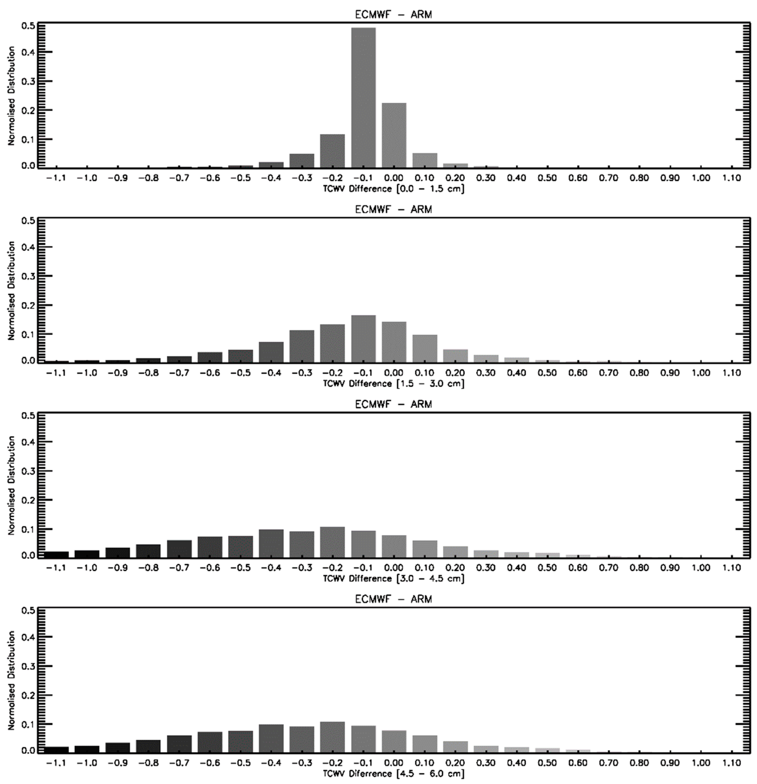
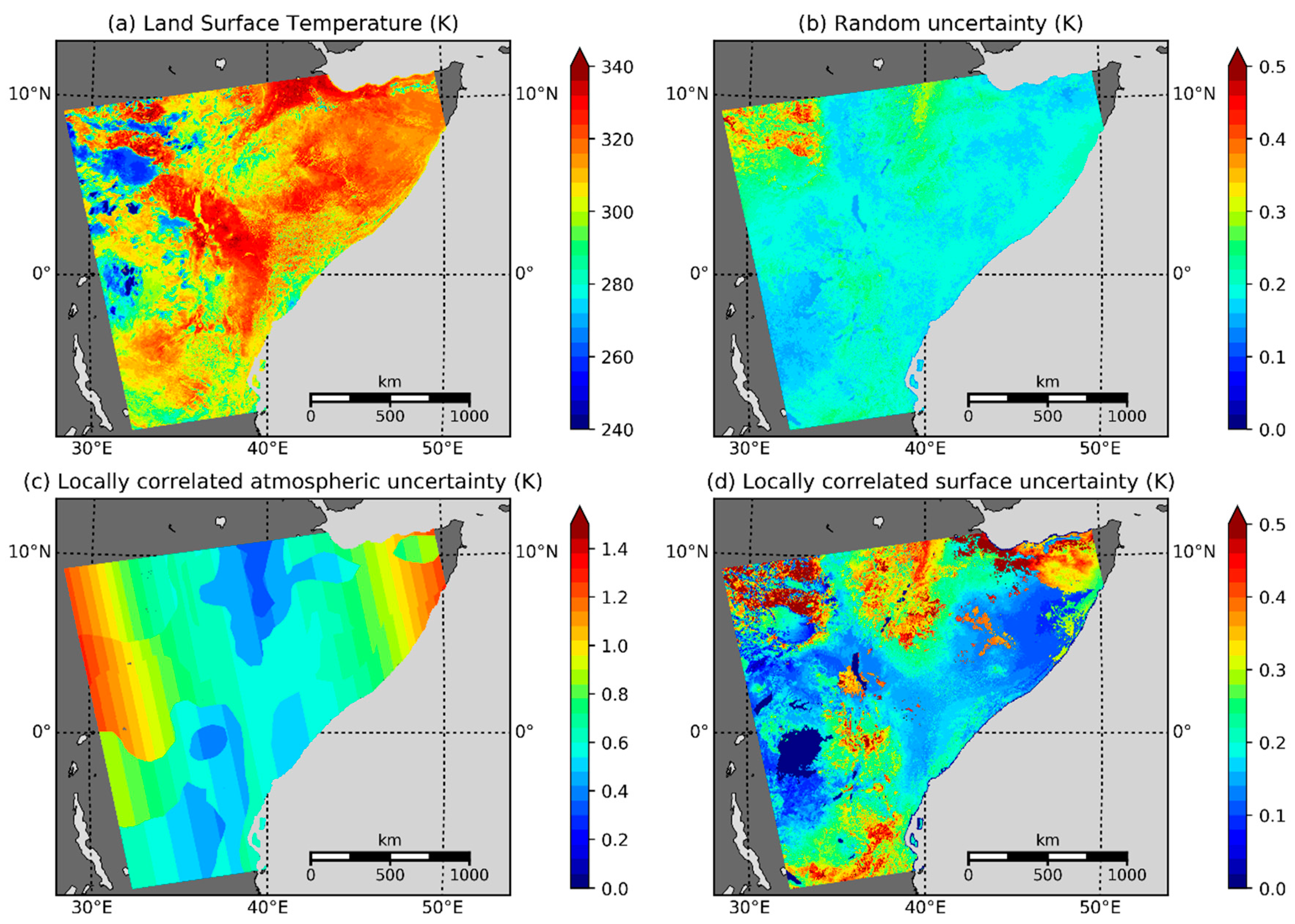
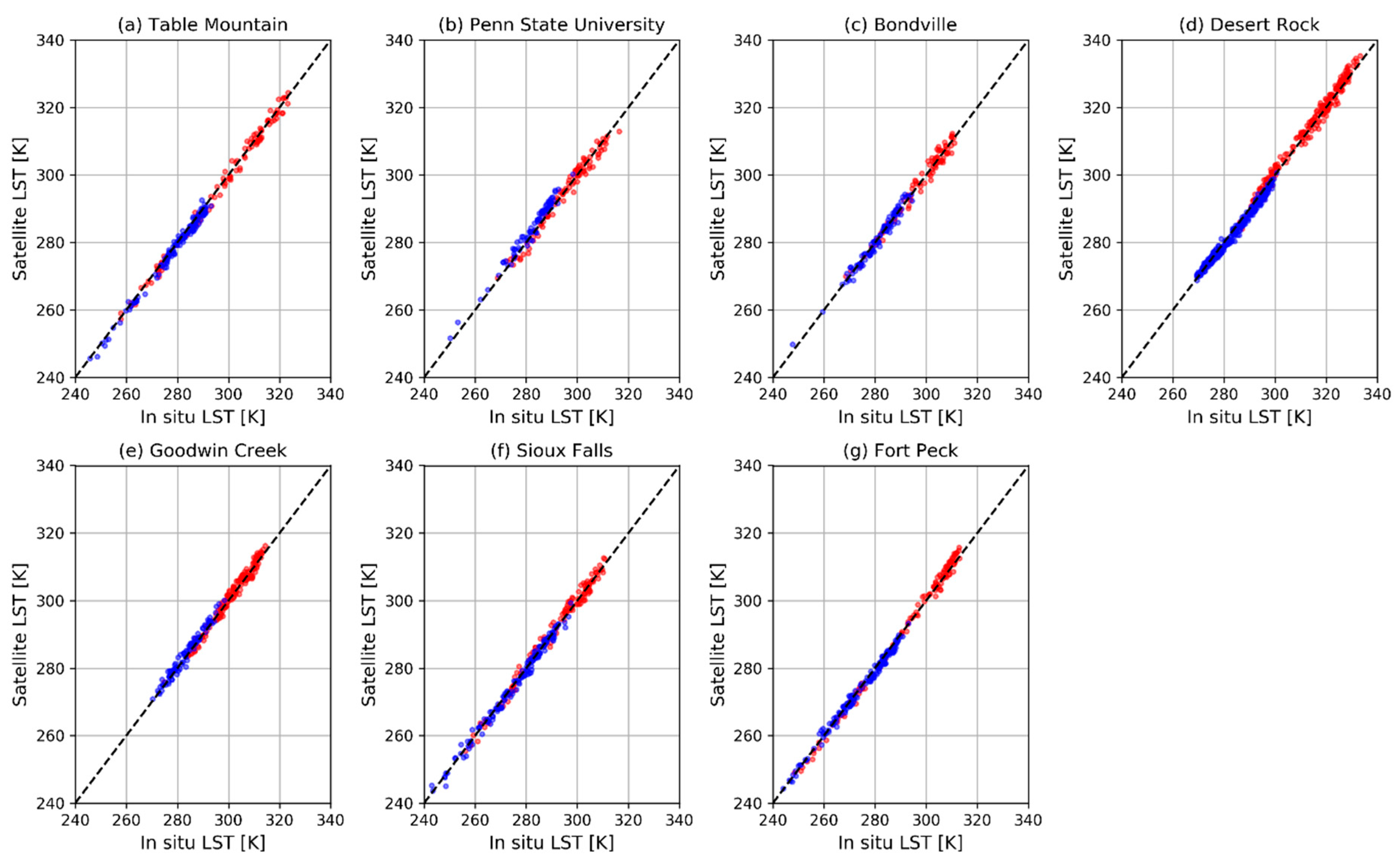
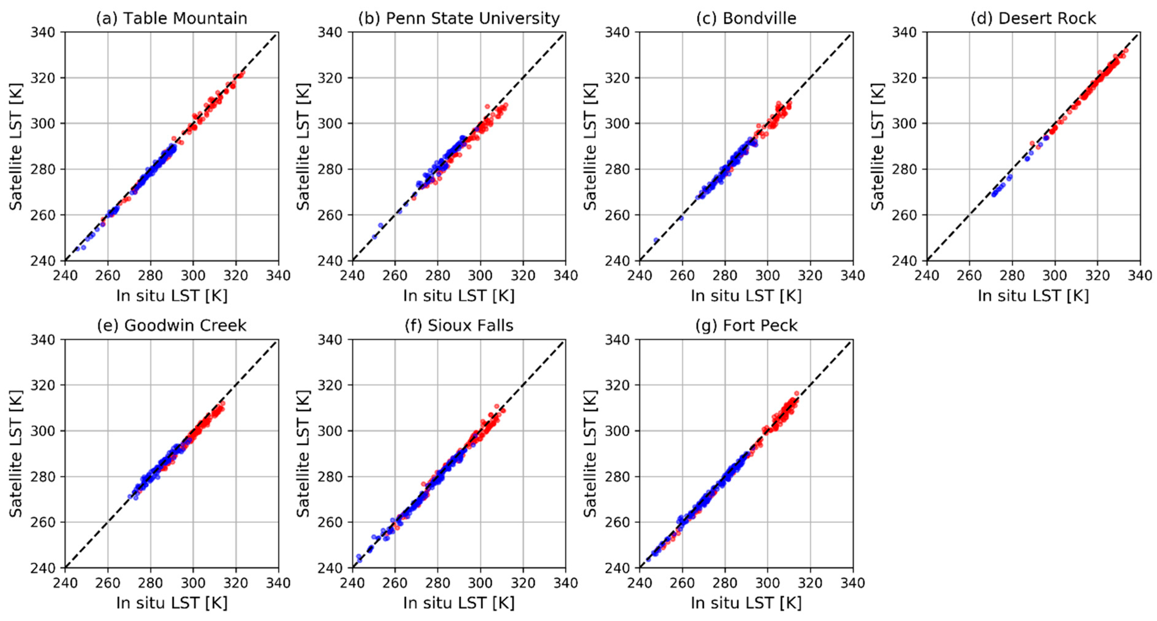
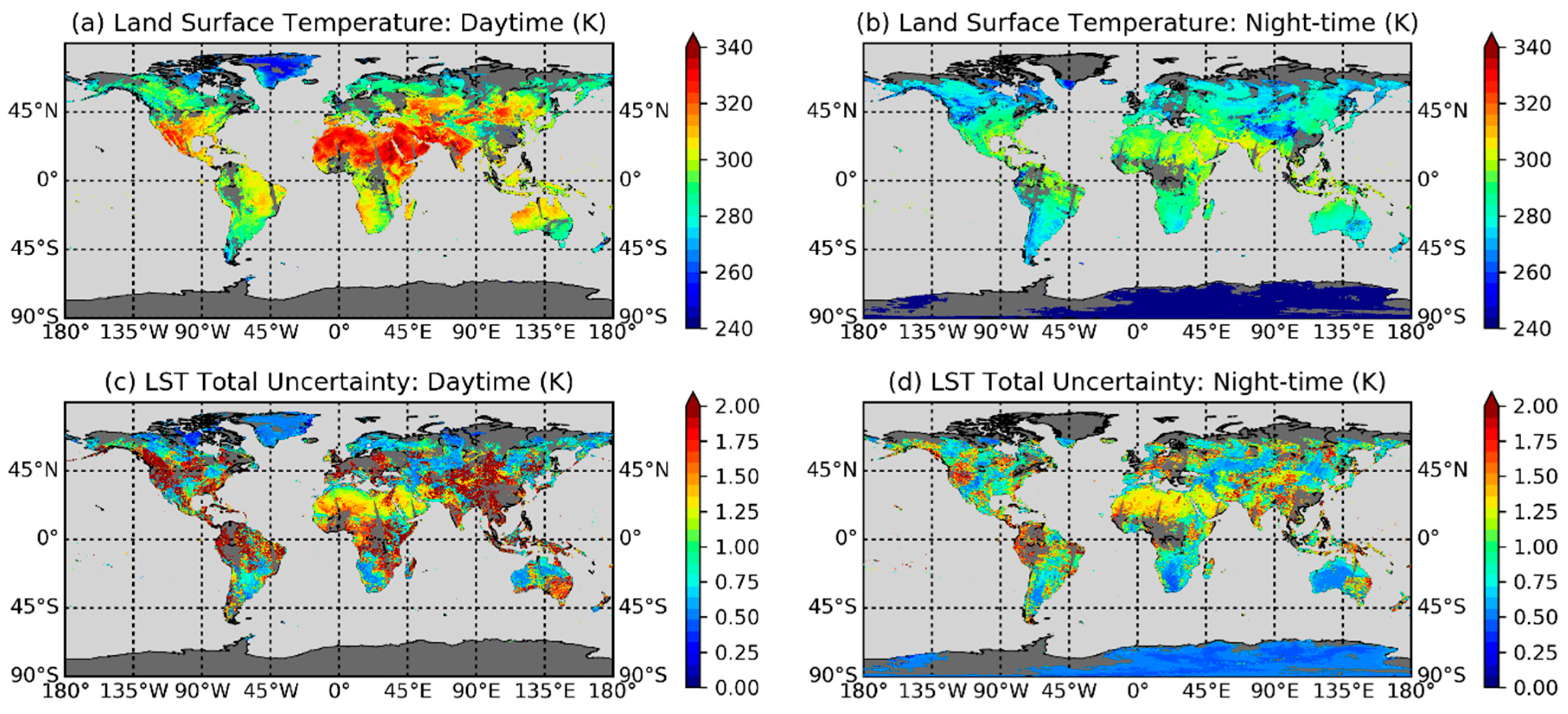
Table 1.
Characteristics of the in situ stations of the Surface Radiation (SURFRAD) network.
| Site | Latitude | Longitude | Elevation | Surface Type | Site |
|---|---|---|---|---|---|
| Bondville | 40.05155 | −88.37325 | 230 m | Grassland | Bondville |
| Desert Rock | 36.62320 | −116.01962 | 1007 m | Arid shrub land | Desert Rock |
| Fort Peck | 48.30798 | −105.10177 | 634 m | Grassland | Fort Peck |
| Goodwin Creek | 34.2547 | −89.8729 | 98 m | Grassland | Goodwin Creek |
| Penn State University | 40.72033 | −77.93100 | 376 m | Cropland | Penn State University |
| Sioux Falls | 43.73431 | −96.62334 | 473 m | Grassland | Sioux Falls |
| Table Mountain | 40.12557 | −105.23775 | 1689 m | Sparse grassland | Table Mountain |
Table 2.
In situ validation statistics during 2011 for both GlobTemperature Aqua-MODIS LST retrievals (GT_MYD_2P) and operational Aqua-MODIS LST retrievals (MYD11_L2) with respect to the seven SURFRAD sites. Number of matchups (n), median (μ) differences, robust standard deviations (σ) and root-mean-square errors (RMSEs) are presented for both day and night observations.
| Site | LST Product | Day | Night | ||||||
|---|---|---|---|---|---|---|---|---|---|
| n | μ (K) | σ (K) | RMSE (K) | n | μ (K) | σ (K) | RMSE (K) | ||
| Bondville | MYD11_L2 | 74 | −1.16 | 1.74 | 2.09 | 92 | −0.51 | 1.38 | 1.47 |
| GT_MYD_2P | 84 | 0.08 | 1.66 | 1.66 | 93 | 0.02 | 1.33 | 1.33 | |
| Desert Rock | MYD11_L2 | 101 | −1.57 | 0.85 | 1.78 | 16 | −2.36 | 0.23 | 2.37 |
| GT_MYD_2P | 219 | 0.87 | 1.48 | 1.71 | 270 | −0.88 | 1.17 | 1.46 | |
| Fort Peck | MYD11_L2 | 116 | −0.68 | 1.60 | 1.74 | 167 | −0.63 | 1.06 | 1.23 |
| GT_MYD_2P | 107 | 0.28 | 1.43 | 1.46 | 166 | −0.42 | 1.09 | 1.17 | |
| Goodwin Creek | MYD11_L2 | 113 | −1.91 | 1.06 | 2.18 | 90 | −0.08 | 1.41 | 1.41 |
| GT_MYD_2P | 138 | 0.31 | 1.38 | 1.42 | 89 | 0.86 | 1.21 | 1.49 | |
| Penn State University | MYD11_L2 | 82 | −2.20 | 1.67 | 2.76 | 76 | 0.75 | 1.47 | 1.65 |
| GT_MYD_2P | 91 | −0.28 | 1.66 | 1.68 | 73 | 1.85 | 1.37 | 2.31 | |
| Sioux Falls | MYD11_L2 | 110 | −0.84 | 1.69 | 1.89 | 139 | −0.88 | 1.27 | 1.55 |
| GT_MYD_2P | 120 | 0.35 | 1.63 | 1.67 | 142 | −0.29 | 1.26 | 1.30 | |
| Table Mountain | MYD11_L2 | 87 | −0.96 | 1.40 | 1.70 | 121 | −1.23 | 0.84 | 1.49 |
| GT_MYD_2P | 102 | −0.40 | 1.45 | 1.50 | 136 | −0.77 | 1.06 | 1.31 | |
© 2019 by the authors. Licensee MDPI, Basel, Switzerland. This article is an open access article distributed under the terms and conditions of the Creative Commons Attribution (CC BY) license (http://creativecommons.org/licenses/by/4.0/).
Share and Cite
MDPI and ACS Style
Ghent, D.; Veal, K.; Trent, T.; Dodd, E.; Sembhi, H.; Remedios, J. A New Approach to Defining Uncertainties for MODIS Land Surface Temperature. Remote Sens. 2019, 11, 1021. https://0-doi-org.brum.beds.ac.uk/10.3390/rs11091021
AMA Style
Ghent D, Veal K, Trent T, Dodd E, Sembhi H, Remedios J. A New Approach to Defining Uncertainties for MODIS Land Surface Temperature. Remote Sensing. 2019; 11(9):1021. https://0-doi-org.brum.beds.ac.uk/10.3390/rs11091021
Chicago/Turabian StyleGhent, Darren, Karen Veal, Tim Trent, Emma Dodd, Harjinder Sembhi, and John Remedios. 2019. "A New Approach to Defining Uncertainties for MODIS Land Surface Temperature" Remote Sensing 11, no. 9: 1021. https://0-doi-org.brum.beds.ac.uk/10.3390/rs11091021
Note that from the first issue of 2016, this journal uses article numbers instead of page numbers. See further details here.