Three-Dimensional Reconstruction of Structural Surface Model of Heritage Bridges Using UAV-Based Photogrammetric Point Clouds


Abstract
:1. Introduction
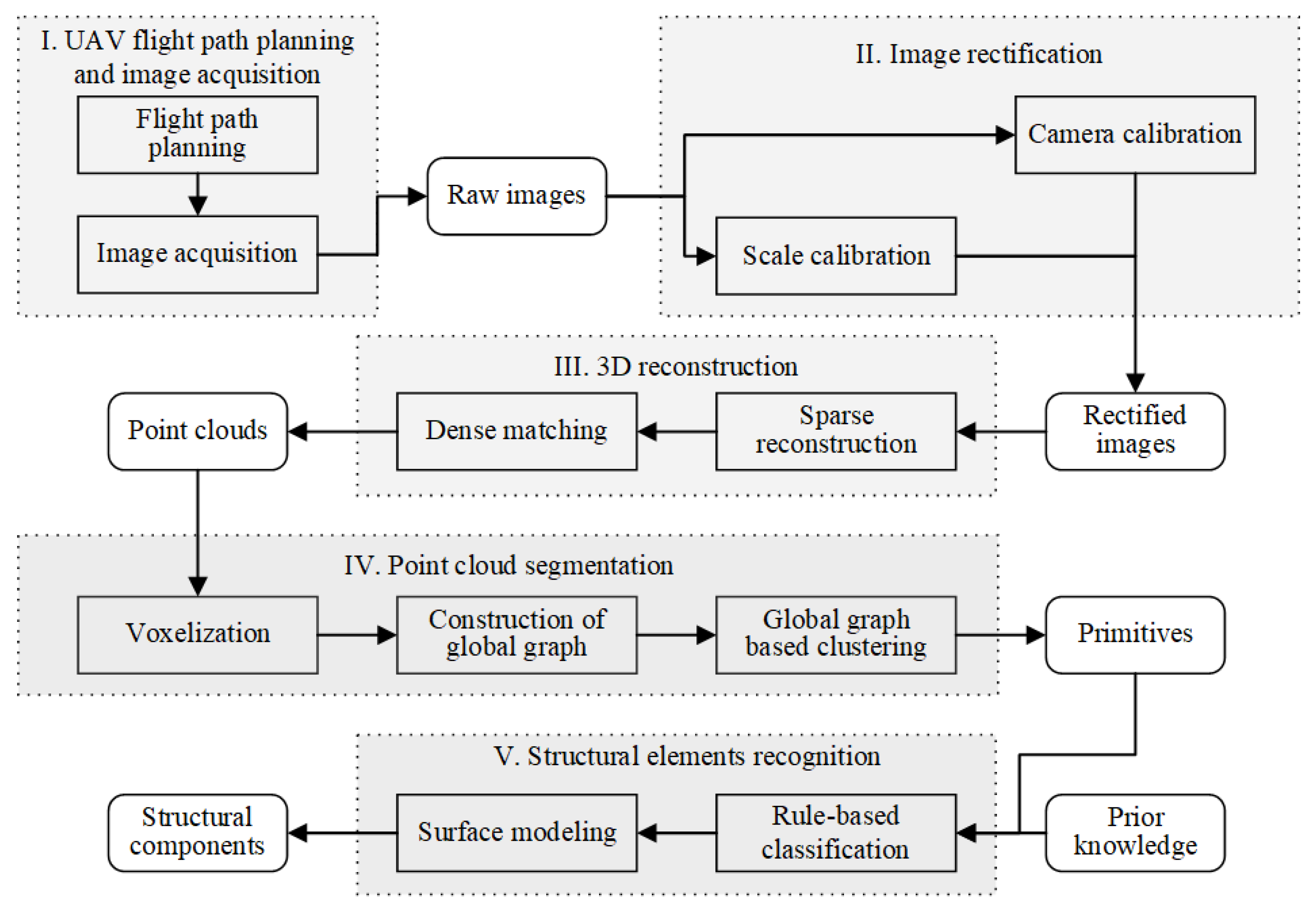
2. Methodology
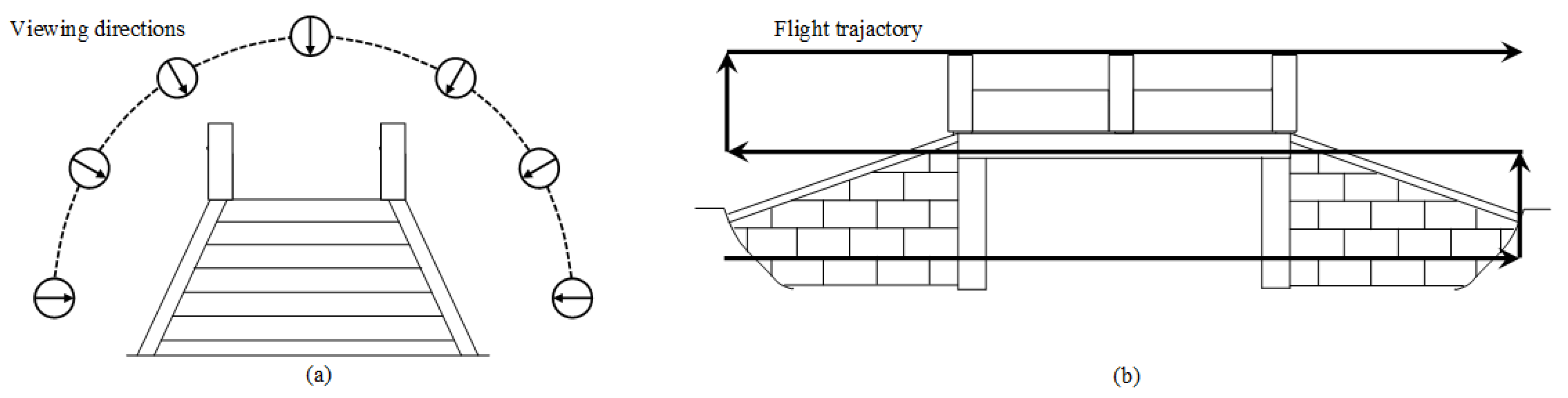
2.1. UAV Flight Path Planning and Image Acquisition
- Shooting according to a serpentine route;
- The overlap ratio of the heading should be greater than 60%, and 90% is recommended;
- The side overlap ratio should be greater than 30%, and 60% is recommended.
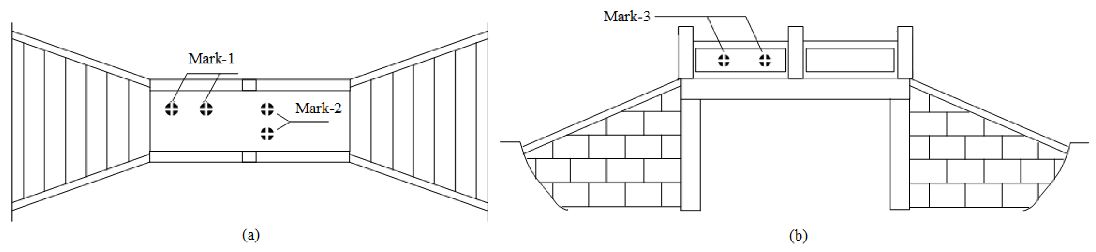
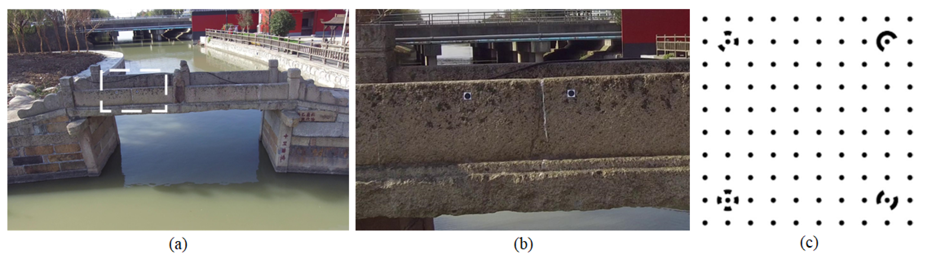
2.2. Image Rectification
2.3. 3D Reconstruction
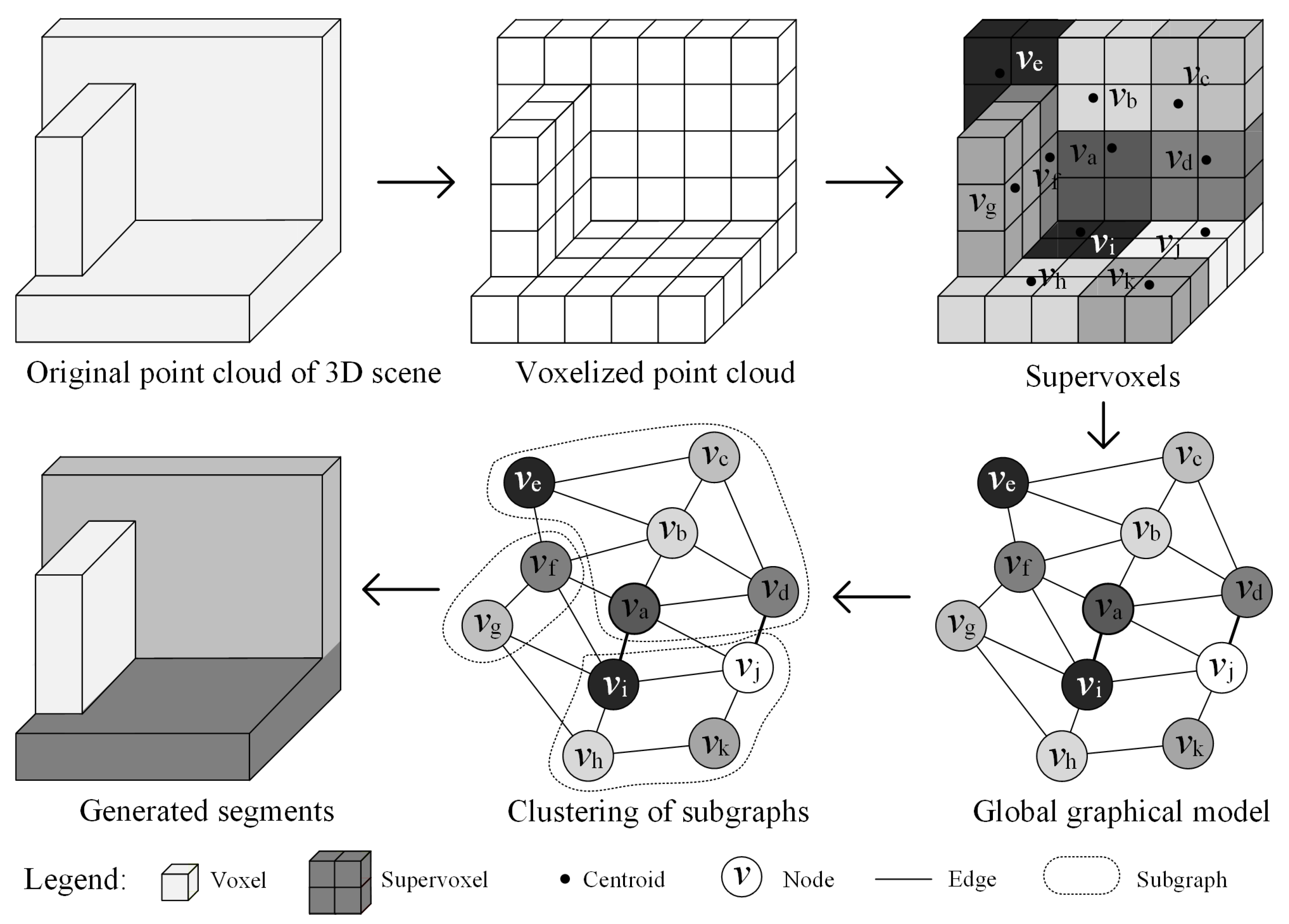
2.4. Point Cloud Segmentation
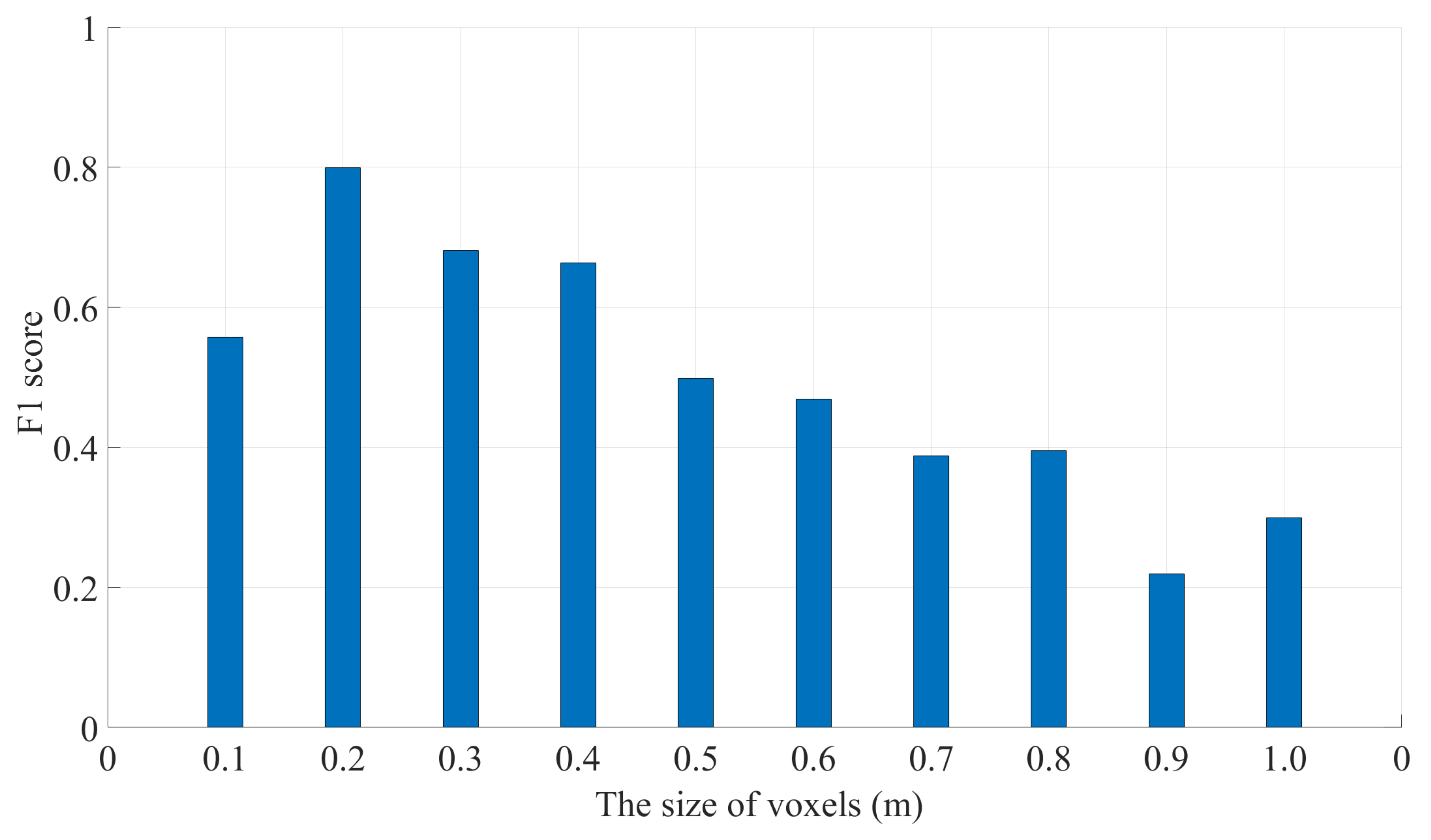
2.4.1. Supervoxelization of Point Clouds
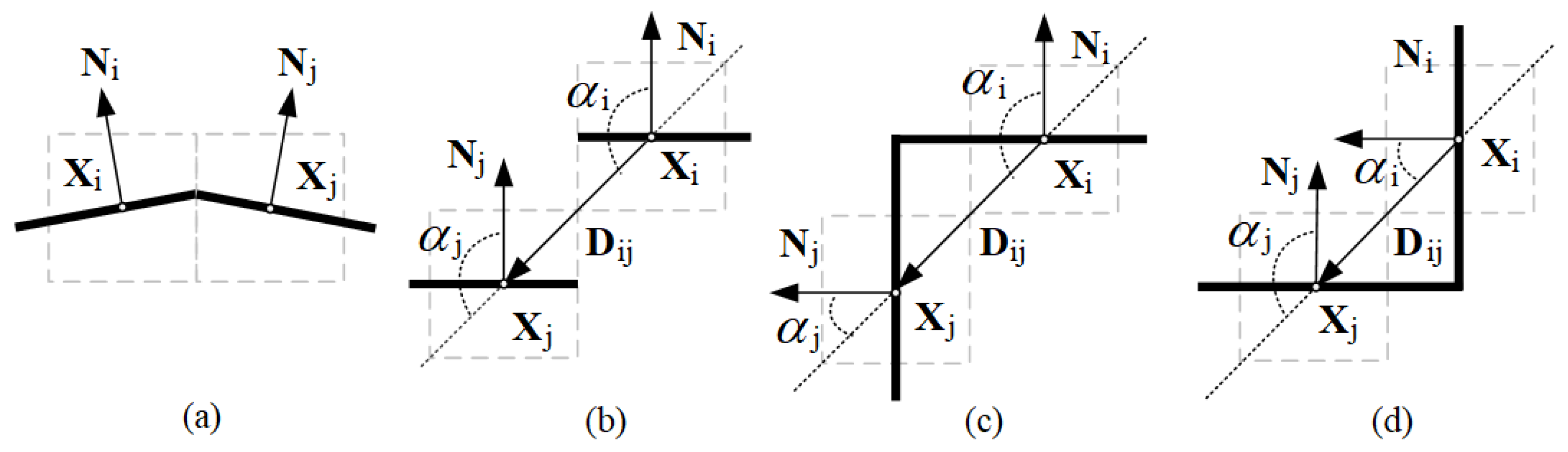
2.4.2. Construction of Global Graph
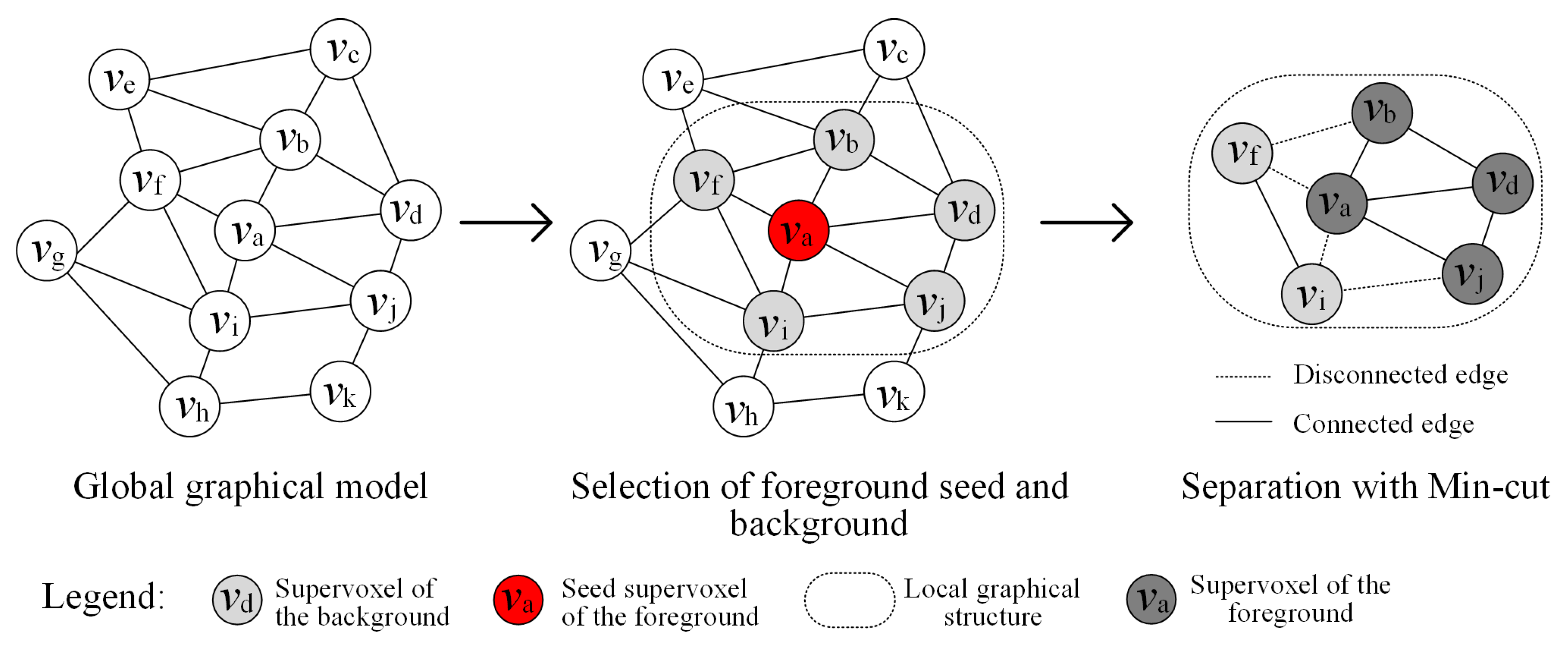
2.4.3. Global Graph-Based Clustering
2.5. Structural Element Recognition
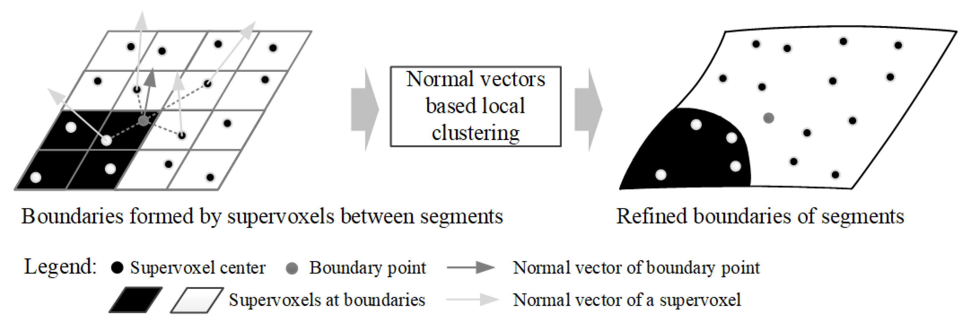
2.5.1. Refinement of Segments
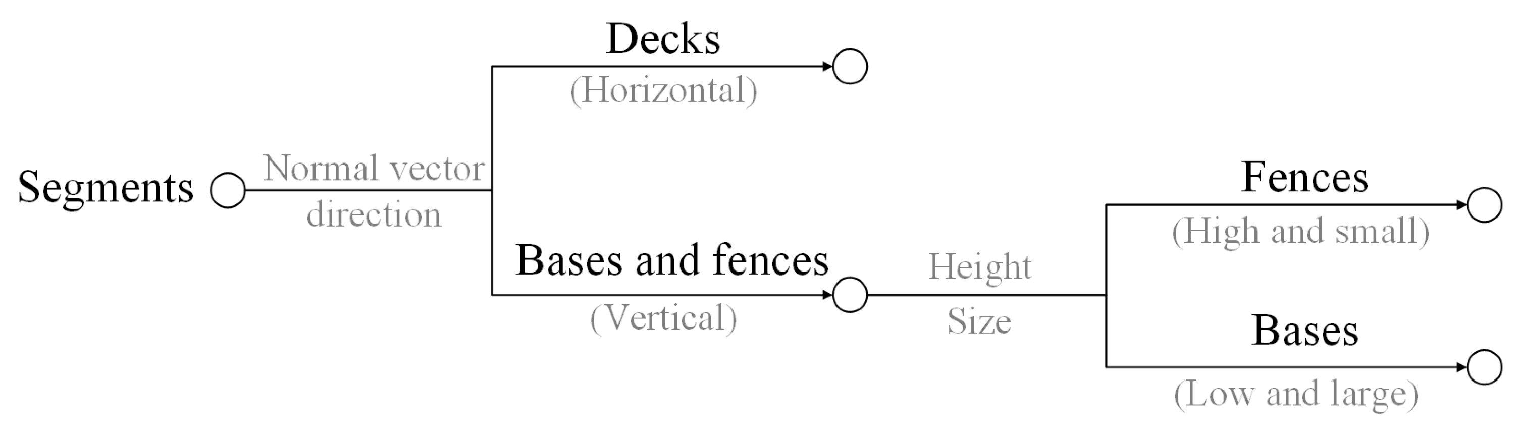
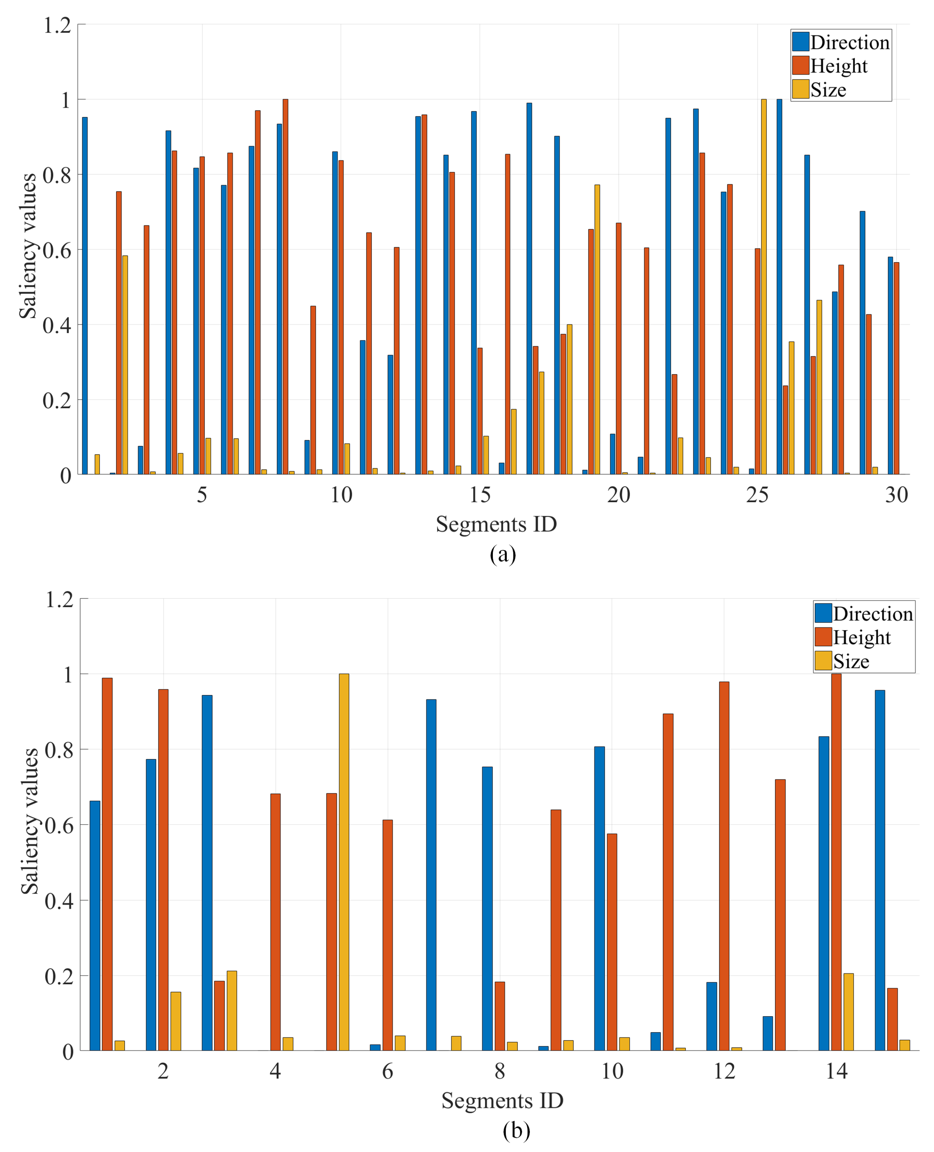
2.5.2. Recognition of Elements
- The height indicating the spatial position;
- The angle between the horizontal direction and the normal vector of the segment;
- The size of segments relating to the spatial length, width, and height.
2.5.3. Surface Modeling
3. Results and Discussion
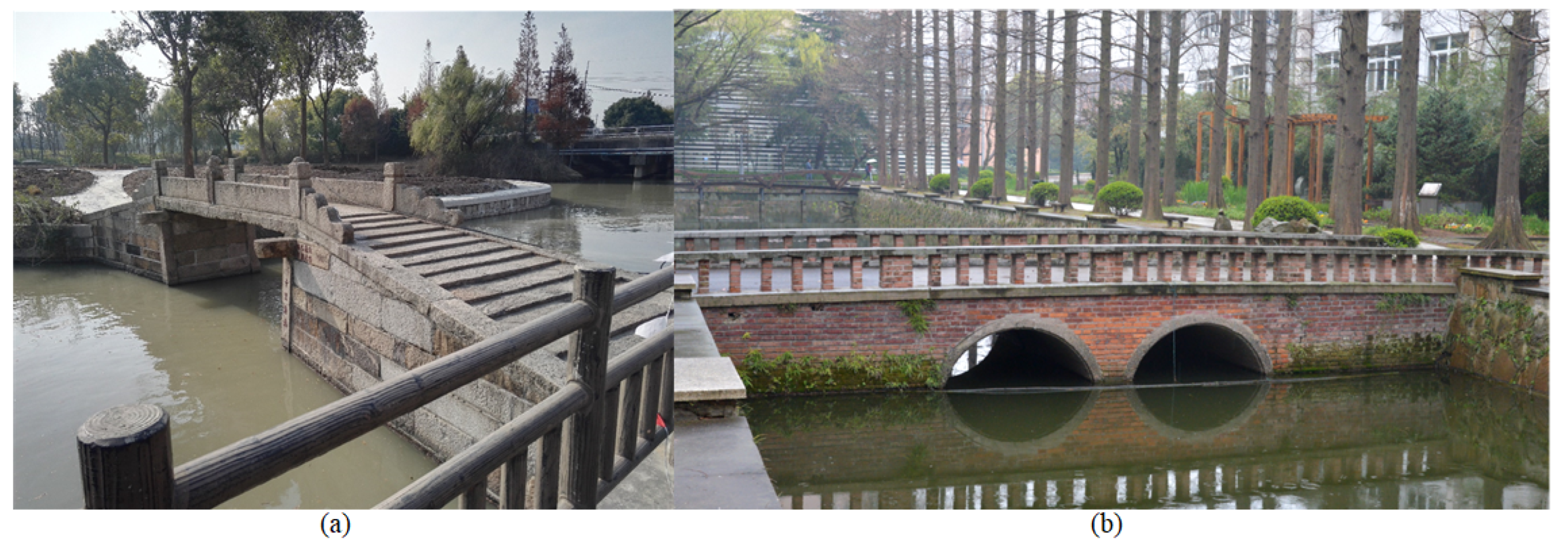
3.1. Testing Data of Bridges
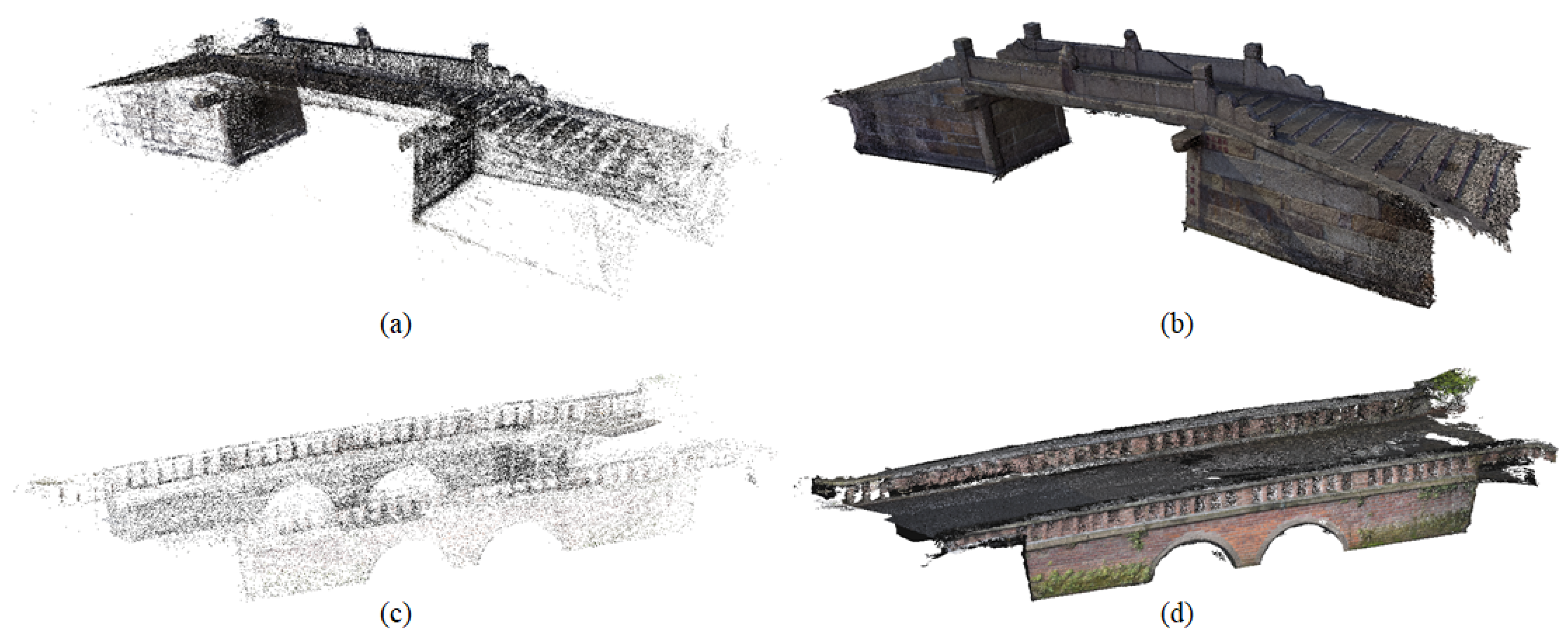
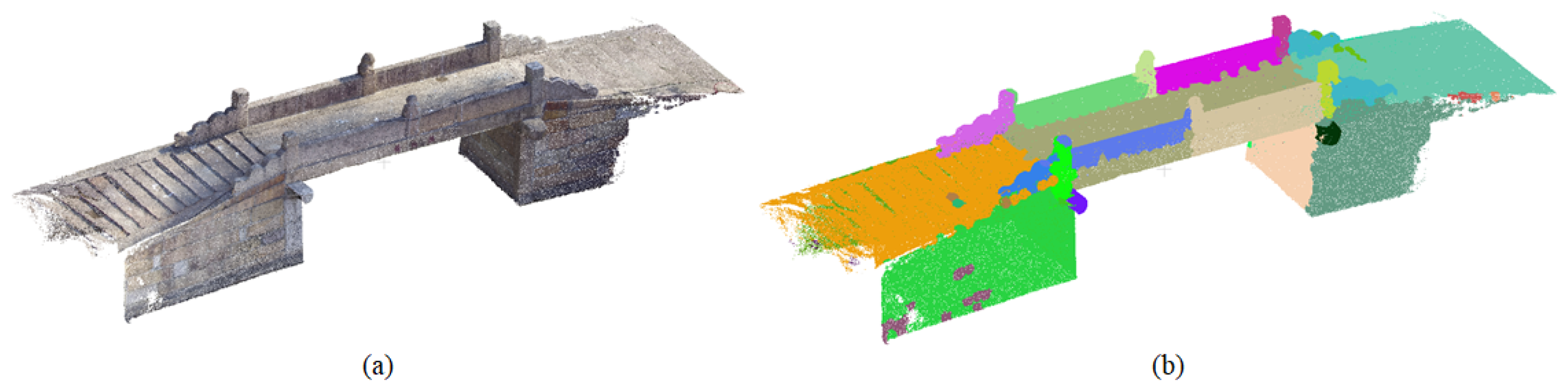
3.2. Generated Point Clouds
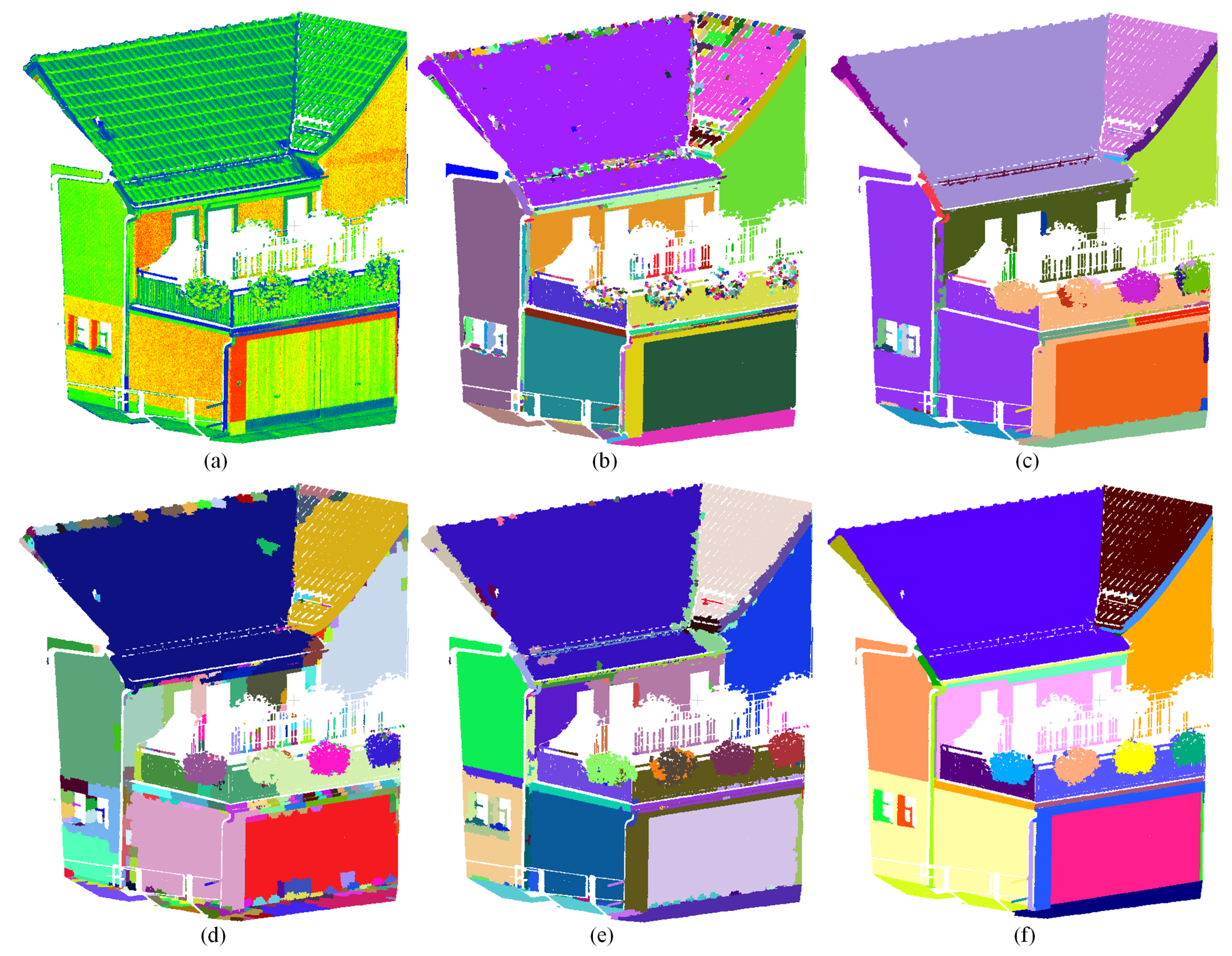
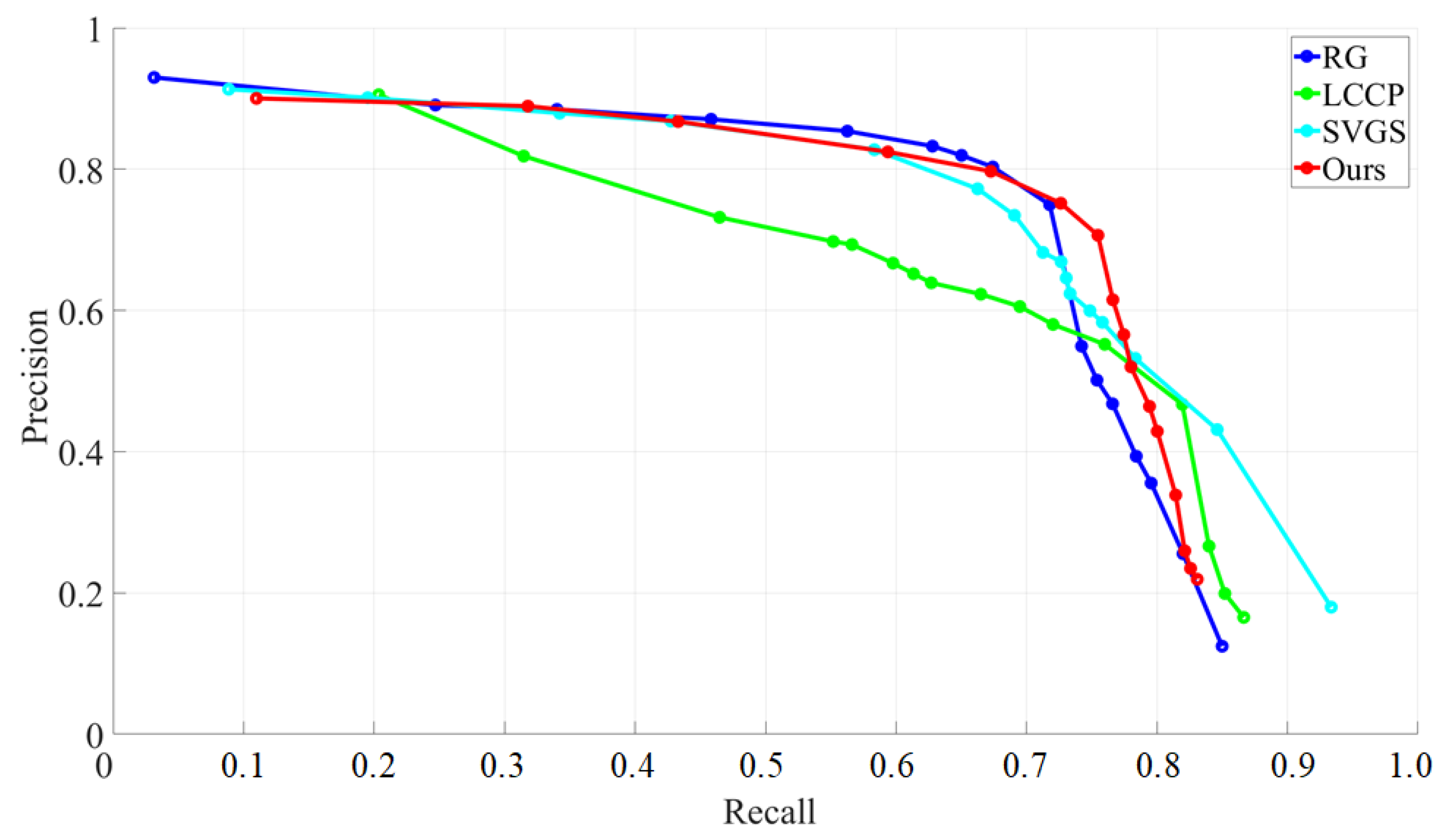
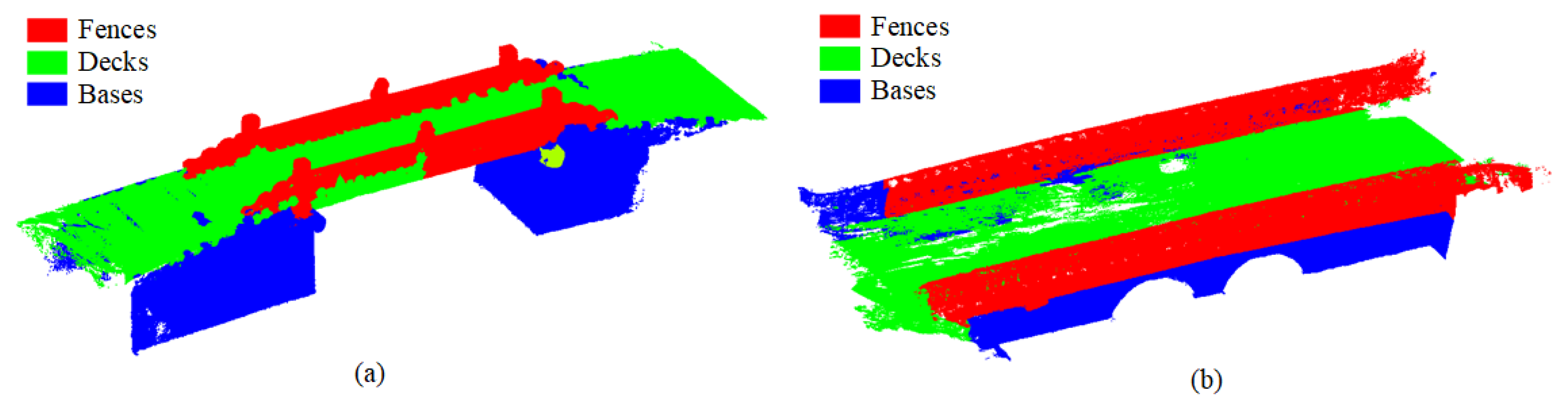
3.3. Quality of Segmentation
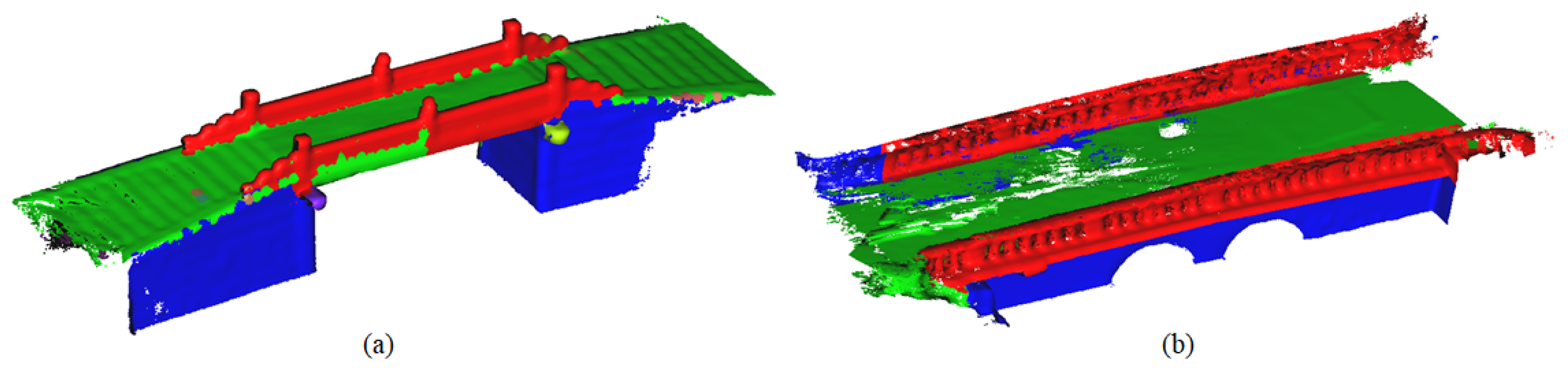
3.4. Recognition and Modeling of Structural Elements
4. Conclusions
Author Contributions
Funding
Conflicts of Interest
References
- Murtiyoso, A.; Grussenmeyer, P. Documentation of heritage buildings using close-range UAV images: Dense matching issues, comparison and case studies. Photogramm. Rec. 2017, 32, 206–229. [Google Scholar] [CrossRef]
- Jiang, S.; Jiang, W. Efficient sfm for oblique uav images: From match pair selection to geometrical verification. Remote. Sens. 2018, 10, 1246. [Google Scholar] [CrossRef]
- Watts, A.C.; Ambrosia, V.G.; Hinkley, E.A. Unmanned aircraft systems in remote sensing and scientific research: Classification and considerations of use. Remote. Sens. 2012, 4, 1671–1692. [Google Scholar] [CrossRef]
- Colomina, I.; Molina, P. Unmanned aerial systems for photogrammetry and remote sensing: A review. ISPRS J. Photogramm. Remote. Sens. 2014, 92, 79–97. [Google Scholar] [CrossRef] [Green Version]
- Nex, F.; Remondino, F. UAV for 3D mapping applications: A review. Appl. Geomat. 2014, 6, 1–15. [Google Scholar] [CrossRef]
- Fernández-Hernandez, J.; González-Aguilera, D.; Rodríguez-Gonzálvez, P.; Mancera-Taboada, J. Image-based modelling from unmanned aerial vehicle (UAV) photogrammetry: An effective, low-cost tool for archaeological applications. Archaeometry 2015, 57, 128–145. [Google Scholar] [CrossRef]
- Liu, S.; Tong, X.; Chen, J.; Liu, X.; Sun, W.; Xie, H.; Chen, P.; Jin, Y.; Ye, Z. A Linear Feature-Based Approach for the Registration of Unmanned Aerial Vehicle Remotely-Sensed Images and Airborne LiDAR Data. Remote. Sens. 2016, 8, 82. [Google Scholar] [CrossRef]
- Gevaert, C.; Sliuzas, R.; Persello, C.; Vosselman, G. Evaluating the societal impact of using drones to support urban upgrading projects. ISPRS Int. J. -Geo-Inf. 2018, 7, 91. [Google Scholar] [CrossRef]
- Bhardwaj, A.; Sam, L.; Martín-Torres, F.J.; Kumar, R. UAVs as remote sensing platform in glaciology: Present applications and future prospects. Remote. Sens. Environ. 2016, 175, 196–204. [Google Scholar] [CrossRef]
- Lottes, P.; Khanna, R.; Pfeifer, J.; Siegwart, R.; Stachniss, C. UAV-based crop and weed classification for smart farming. In Proceedings of the 2017 IEEE International Conference on Robotics and Automation (ICRA), Singapore, 29 May–3 June 2017; pp. 3024–3031. [Google Scholar]
- Manfreda, S.; McCabe, M.; Miller, P.; Lucas, R.; Pajuelo Madrigal, V.; Mallinis, G.; Ben Dor, E.; Helman, D.; Estes, L.; Ciraolo, G.; et al. On the use of unmanned aerial systems for environmental monitoring. Remote. Sens. 2018, 10, 641. [Google Scholar] [CrossRef]
- Chen, P.; Dang, Y.; Liang, R.; Zhu, W.; He, X. Real-time object tracking on a drone with multi-inertial sensing data. IEEE Trans. Intell. Transp. Syst. 2018, 19, 131–139. [Google Scholar] [CrossRef]
- Lucieer, A.; Jong, S.M.D.; Turner, D. Mapping landslide displacements using Structure from Motion (SfM) and image correlation of multi-temporal UAV photography. Prog. Phys. Geogr. 2014, 38, 97–116. [Google Scholar] [CrossRef]
- Ewertowski, M.; Tomczyk, A.; Evans, D.; Roberts, D.; Ewertowski, W. Operational Framework for Rapid, Very-high Resolution Mapping of Glacial Geomorphology Using Low-cost Unmanned Aerial Vehicles and Structure-from-Motion Approach. Remote. Sens. 2019, 11, 65. [Google Scholar] [CrossRef]
- Rakha, T.; Gorodetsky, A. Review of Unmanned Aerial System (UAS) applications in the built environment: Towards automated building inspection procedures using drones. Autom. Constr. 2018, 93, 252–264. [Google Scholar] [CrossRef]
- Kohv, M.; Sepp, E.; Vammus, L. Assessing multitemporal water-level changes with uav-based photogrammetry. Photogramm. Rec. 2017, 32, 424–442. [Google Scholar] [CrossRef] [Green Version]
- He, F.; Zhou, T.; Xiong, W.; Hasheminnasab, S.; Habib, A. Automated aerial triangulation for UAV-based mapping. Remote. Sens. 2018, 10, 1952. [Google Scholar] [CrossRef]
- He, F.; Habib, A. Automated relative orientation of UAV-based imagery in the presence of prior information for the flight trajectory. Photogramm. Eng. Remote. Sens. 2016, 82, 879–891. [Google Scholar] [CrossRef]
- Habib, A.; Xiong, W.; He, F.; Yang, H.L.; Crawford, M. Improving orthorectification of UAV-based push-broom scanner imagery using derived orthophotos from frame cameras. IEEE J. Sel. Top. Appl. Earth Obs. Remote. Sens. 2017, 10, 262–276. [Google Scholar] [CrossRef]
- Ye, Z.; Tong, X.; Zheng, S.; Guo, C.; Gao, S.; Liu, S.; Xu, X.; Jin, Y.; Xie, H.; Liu, S.; et al. Illumination-Robust Subpixel Fourier-Based Image Correlation Methods Based on Phase Congruency. IEEE Trans. Geosci. Remote. Sens. 2018, 1995–2008. [Google Scholar] [CrossRef]
- Khaloo, A.; Lattanzi, D.; Cunningham, K.; Dell’Andrea, R.; Riley, M. Unmanned aerial vehicle inspection of the Placer River Trail Bridge through image-based 3D modelling. Struct. Infrastruct. Eng. 2018, 14, 124–136. [Google Scholar] [CrossRef]
- Morgenthal, G.; Hallermann, N.; Kersten, J.; Taraben, J.; Debus, P.; Helmrich, M.; Rodehorst, V. Framework for automated UAS-based structural condition assessment of bridges. Autom. Constr. 2019, 97, 77–95. [Google Scholar] [CrossRef]
- Chen, S.; Laefer, D.F.; Mangina, E.; Zolanvari, S.I.; Byrne, J. UAV Bridge Inspection through Evaluated 3D Reconstructions. J. Bridge Eng. 2019, 24, 05019001. [Google Scholar] [CrossRef] [Green Version]
- Xu, Y.; Tuttas, S.; Heogner, L.; Stilla, U. Reconstruction of scaffolds from a photogrammetric point cloud of construction sites using a novel 3D local feature descriptor. Autom. Constr. 2018, 85. [Google Scholar] [CrossRef]
- Xu, Y.; Tuttas, S.; Hoegner, L.; Stilla, U. Geometric Primitive Extraction From Point Clouds of Construction Sites Using VGS. IEEE Geosci. Remote. Sens. Lett. 2017, 14, 424–428. [Google Scholar] [CrossRef]
- Grilli, E.; Menna, F.; Remondino, F. A review of point clouds segmentation and classification algorithms. ISPRS Int. Arch. Photogramm. Remote. Sens. Spat. Inf. Sci. 2017, XLII-2/W3, 339–344. [Google Scholar] [CrossRef]
- Aldoma, A.; Marton, Z.C.; Tombari, F.; Wohlkinger, W.; Potthast, C.; Zeisl, B.; Rusu, R.; Gedikli, S.; Vincze, M. Tutorial: Point cloud library: Three-dimensional object recognition and 6 dof pose estimation. IEEE Robot. Autom. Mag. 2012, 19, 80–91. [Google Scholar] [CrossRef]
- Lu, X.; Yao, J.; Tu, J.; Li, K.; Li, L.; Liu, Y. Pairwise linkage for point cloud segmentation. ISPRS Ann. Photogramm. Remote. Sens. Spat. Inf. Sci. 2016, III-3, 201–208. [Google Scholar] [CrossRef]
- Aljumaily, H.; Laefer, D.F.; Cuadra, D. Urban point cloud mining based on density clustering and mapreduce. J. Comput. Civ. Eng. 2017, 31, 04017021. [Google Scholar] [CrossRef]
- Vo, A.V.; Truong-Hong, L.; Laefer, D.F.; Bertolotto, M. Octree-based region growing for point cloud segmentation. ISPRS J. Photogramm. Remote. Sens. 2015, 104, 88–100. [Google Scholar] [CrossRef]
- Tóvári, D.; Pfeifer, N. Segmentation based robust interpolation-a new approach to laser data filtering. ISPRS Int. Arch. Photogramm. Remote. Sens. Spat. Inf. Sci. 2005, 36, 79–84. [Google Scholar]
- Rabbani, T.; Van Den Heuvel, F.; Vosselmann, G. Segmentation of point clouds using smoothness constraint. ISPRS Int. Arch. Photogramm. Remote. Sens. Spat. Inf. Sci. 2006, 36, 248–253. [Google Scholar]
- Besl, P.; Jain, R. Segmentation through variable-order surface fitting. IEEE Trans. Pattern Anal. Mach. Intell. 1988, 10, 167–192. [Google Scholar] [CrossRef]
- Nurunnabi, A.; Belton, D.; West, G. Robust segmentation for large volumes of laser scanning three-dimensional point cloud data. IEEE Trans. Geosci. Remote. Sens. 2016, 54, 4790–4805. [Google Scholar] [CrossRef]
- Harwin, S.; Lucieer, A.; Osborn, J. The impact of the calibration method on the accuracy of point clouds derived using unmanned aerial vehicle multi-view stereopsis. Remote. Sens. 2015, 7, 11933–11953. [Google Scholar] [CrossRef]
- Brown, D.C. Close-range camera calibration. Photogramm. Eng. 1971, 37, 855–866. [Google Scholar]
- Eltner, A.; Kaiser, A.; Castillo, C.; Rock, G.; Neugirg, F.; Abellán, A. Image-based surface reconstruction in geomorphometry–merits, limits and developments. Earth Surf. Dyn. 2016, 4, 359–389. [Google Scholar] [CrossRef]
- Verhoeven, G. Taking computer vision aloft–archaeological three-dimensional reconstructions from aerial photographs with photoscan. Archaeol. Prospect. 2011, 18, 67–73. [Google Scholar] [CrossRef]
- Rusu, R.B.; Cousins, S. 3D is here: Point cloud library (pcl). In Proceedings of the IEEE International Conference on Robotics and Automation, Shanghai, China, 9–13 May 2011; pp. 1–4. [Google Scholar] [CrossRef]
- Xu, Y.; Yao, W.; Tuttas, S.; Hoegner, L.; Stilla, U. Unsupervised segmentation of point clouds from buildings using hierarchical clustering based on gestalt principles. IEEE J. Sel. Top. Appl. Earth Obs. Remote. Sens. 2018, 1–17. [Google Scholar] [CrossRef]
- Papon, J.; Abramov, A.; Schoeler, M.; Worgotter, F. Voxel cloud connectivity segmentation-supervoxels for point clouds. In Proceedings of the IEEE Conference on Computer Vision and Pattern Recognition, Portland, OR, USA, 23–28 June 2013; pp. 2027–2034. [Google Scholar] [CrossRef]
- Xu, Y.; Heogner, L.; Tuttas, S.; Stilla, U. A voxel- and graph-based strategy for segmenting man-made infrastructures using perceptual grouping laws: Comparison and evaluation. Photogramm. Eng. Remote. Sens. 2018. [Google Scholar] [CrossRef]
- Weinmann, M.; Jutzi, B.; Hinz, S.; Mallet, C. Semantic point cloud interpretation based on optimal neighborhoods, relevant features and efficient classifiers. ISPRS J. Photogramm. Remote. Sens. 2015, 105, 286–304. [Google Scholar] [CrossRef]
- Stein, S.C.; Schoeler, M.; Papon, J.; Worgotter, F. Object partitioning using local convexity. In Proceedings of the IEEE Conference on Computer Vision and Pattern Recognition, Columbus, OH, USA, 23–28 June 2014; pp. 304–311. [Google Scholar] [CrossRef]
- Xu, Y.; Yao, W.; Hoegner, L.; Stilla, U. Segmentation of Building Roofs from Airborne LiDAR Point Clouds Using Robust Voxel-Based Region Growing. Remote. Sens. Lett. 2017, 8, 1062–1071. [Google Scholar] [CrossRef]
- Peng, B.; Zhang, L.; Zhang, D. A survey of graph theoretical approaches to image segmentation. Pattern Recognit. 2013, 46, 1020–1038. [Google Scholar] [CrossRef]
- Yao, W.; Hinz, S.; Stilla, U. Automatic vehicle extraction from airborne LiDAR data of urban areas aided by geodesic morphology. Pattern Recognit. Lett. 2010, 31, 1100–1108. [Google Scholar] [CrossRef]
- Funkhouser, T.; Golovinsky, A. Min-cut based segmentation of point clouds. In Proceedings of the 2009 IEEE 12th International Conference on Computer Vision Workshops (ICCV Workshops), Kyoto, Japan, 27 September–4 October 2009; pp. 39–46. [Google Scholar]
- Sun, Z.; Xu, Y.; Hoegner, L.; Stilla, U. Classification of MLS point clouds in urban scenes using detrended geometric features from supervoxel-based local context. ISPRS Ann. Photogramm. Remote. Sens. Spat. Inf. Sci. 2018, IV-2, 271–278. [Google Scholar] [CrossRef]
- Yang, B.; Dong, Z.; Zhao, G.; Dai, W. Hierarchical extraction of urban objects from mobile laser scanning data. ISPRS J. Photogramm. Remote. Sens. 2015, 99, 45–57. [Google Scholar] [CrossRef]
- Kazhdan, M.; Bolitho, M.; Hoppe, H. Poisson surface reconstruction. In Proceedings of the Fourth Eurographics Symposium on Geometry Processing, Sardinia, Italy, 26–28 June 2006; Volume 7. [Google Scholar]


| Scale | UAV Distance to Bridge (m) | Measured Distance (m) | Ground Truth Distance (m) | Error |
|---|---|---|---|---|
| Small | 2.0 | 0.504 | 0.5 | 0.8% |
| Middle | 5.0 | 0.515 | 0.5 | 3.0% |
| Large | 8.0 | 0.523 | 0.5 | 4.6% |
| All | – | 0.502 | 0.5 | 0.4% |
| Name | Number of Points | Number of Segments |
|---|---|---|
| Hongde Bridge | 18,114,743 | 30 |
| Tongxin Bridge | 5,613,422 | 15 |
| Name | Total Segments | Segments of Decks | Segments of Bases | Segments of Fences |
|---|---|---|---|---|
| Hongde Bridge | 30 | 8 | 8 | 14 |
| Tongxin Bridge | 15 | 2 | 4 | 9 |
| Hongde Bridge | Tongxin Bridge | ||||||
|---|---|---|---|---|---|---|---|
| Predict | Decks | Bases | Fences | Decks | Bases | Fences | |
| Truth | |||||||
| Decks | 6 | 0 | 2 | 2 | 0 | 0 | |
| Bases | 1 | 8 | 1 | 0 | 3 | 2 | |
| Fences | 1 | 0 | 11 | 0 | 1 | 7 | |
| Overall accuracy (OA) | 0.83 | 0.8 | |||||
© 2019 by the authors. Licensee MDPI, Basel, Switzerland. This article is an open access article distributed under the terms and conditions of the Creative Commons Attribution (CC BY) license (http://creativecommons.org/licenses/by/4.0/).
Share and Cite
Pan, Y.; Dong, Y.; Wang, D.; Chen, A.; Ye, Z. Three-Dimensional Reconstruction of Structural Surface Model of Heritage Bridges Using UAV-Based Photogrammetric Point Clouds. Remote Sens. 2019, 11, 1204. https://0-doi-org.brum.beds.ac.uk/10.3390/rs11101204
Pan Y, Dong Y, Wang D, Chen A, Ye Z. Three-Dimensional Reconstruction of Structural Surface Model of Heritage Bridges Using UAV-Based Photogrammetric Point Clouds. Remote Sensing. 2019; 11(10):1204. https://0-doi-org.brum.beds.ac.uk/10.3390/rs11101204
Chicago/Turabian StylePan, Yue, Yiqing Dong, Dalei Wang, Airong Chen, and Zhen Ye. 2019. "Three-Dimensional Reconstruction of Structural Surface Model of Heritage Bridges Using UAV-Based Photogrammetric Point Clouds" Remote Sensing 11, no. 10: 1204. https://0-doi-org.brum.beds.ac.uk/10.3390/rs11101204