A Fast Global Interpolation Method for Digital Terrain Model Generation from Large LiDAR-Derived Data

Abstract

Airborne light detection and ranging (LiDAR) datasets with a large volume pose a great challenge to the traditional interpolation methods for the production of digital terrain models (DTMs). Thus, a fast, global interpolation method based on thin plate spline (TPS) is proposed in this paper. In the methodology, a weighted version of finite difference TPS is first developed to deal with the problem of missing data in the grid-based surface construction. Then, the interpolation matrix of the weighted TPS is deduced and found to be largely sparse. Furthermore, the values and positions of each nonzero element in the matrix are analytically determined. Finally, to make full use of the sparseness of the interpolation matrix, the linear system is solved with an iterative manner. These make the new method not only fast, but also require less random-access memory. Tests on six simulated datasets indicate that compared to recently developed discrete cosine transformation (DCT)-based TPS, the proposed method has a higher speed and accuracy, lower memory requirement, and less sensitivity to the smoothing parameter. Real-world examples on 10 public and 1 private dataset demonstrate that compared to the DCT-based TPS and the locally weighted interpolation methods, such as linear, natural neighbor (NN), inverse distance weighting (IDW), and ordinary kriging (OK), the proposed method produces visually good surfaces, which overcome the problems of peak-cutting, coarseness, and discontinuity of the aforementioned interpolators. More importantly, the proposed method has a similar performance to the simple interpolation methods (e.g., IDW and NN) with respect to computing time and memory cost, and significantly outperforms OK. Overall, the proposed method with low memory requirement and computing cost offers great potential for the derivation of DTMs from large-scale LiDAR datasets.

1. Introduction

There is little doubt that the acquisition and availability of airborne light detection and ranging (LiDAR) datasets have revolutionized the construction of high-quality digital terrain models (DTMs) [1,2,3], which play an important role in supporting wide range of applications, including engineering projects, geomorphology, hydrology management, and disaster assessment and planning [4]. One promising feature of LiDAR point clouds is the high-density with a large amount of data points. However, this imposes a great challenge on most traditional interpolation methods for the construction of high-resolution and high-quality DTMs [5].

At present, a variety of interpolation methods have been adopted in geosciences for LiDAR-derived DTM generation, such as inverse distance weighting (IDW), triangulated irregular network (TIN) with linear interpolation, natural neighbor (NN), radial basis functions (RBFs), and kriging [6,7,8]. Among them, thin plate spline (TPS), one type of RBF, is highly recommended thanks to its ease of use, flexibility, and high interpolation accuracy. For example, Hutchinson and Gessler [9] suggested that TPS is approximately as accurate for interpolation as kriging, but avoids initial estimation of the covariance structure. Doucette and Beard [10] compared the performance of kriging, TPS, IDW, and surface trend analysis for filling DTM gaps, and found that TPS is more favorable than the others. Desmet [11] showed that the best interpolation method for DTM construction in the selected study area is TPS. Erdogan [12] observed that TPS can obtain the best results for DTM production at the field scale. Additionally, in the context of LiDAR point cloud filtering, TPS was often employed to generate reference ground surfaces [13,14,15,16,17,18].

Nevertheless, like the other RBFs, the wide applicability of TPS was seriously hindered by the huge computational cost. More specifically, using direct methods to solve the TPS system typically requires O(N³) operations and O(N²) storage with N being the number of sample points. As a result, many algorithms have been proposed in recent decades to decrease the computational burden primarily on the basis of three types of schemes: Preconditioner-based fast solution and evaluation, low rank approximation, and domain decomposition. However, these methods are suitable for the analytical TPS. In practice, generating continuous surfaces (e.g., DTMs) can be efficiently achieved by finite difference TPS [19]. Motivated by this idea, we propose a fast, global interpolation method based on finite difference TPS for DTM derivation from large LiDAR datasets.

The main methodological contributions of this paper are as follows: (1) A weighted finite difference TPS is proposed to handle the missing data problem in grid-based surface interpolation, (2) the interpolation matrix of the weighted TPS is deduced and found to be largely sparse. In addition, the values and positions of all nonzero elements of the interpolation matrix are analytically determined, and (3) the sparseness of the interpolation matrix is fully used to solve the linear system of the proposed method. Compared to the existing interpolation methods, the proposed method has the following advantages: (1) Fast by making full use of the sparseness of the linear system; (2) less memory requirement as the elements of the interpolation matrix are known beforehand and do not require the storage; and (3) a global interpolation manner that avoids the discontinuity problem of domain decomposition and local interpolation. The objective of this paper is to first develop a fast, global interpolation method for interpolating large LiDAR data and then assess its performance on simulated and real-world datasets with respect to computing time, accuracy, and memory cost.

The remainder of this paper is organized as follows: Related papers are reviewed in Section 2. Section 3 gives the two basic forms of TPS as the preliminary. Section 4 elaborates the new method. In Section 5, experiments on synthetic and real-world LiDAR datasets to compare the performance of the proposed method and some well-known interpolation methods are given. Discussion and conclusions are shown in Section 6.

2. Literature Review

The existing methods used to reduce the computational cost of TPS interpolation can be generally classified into three groups. The first group is based on the development of preconditioners. For example, Beatson et al. [20] introduced a preconditioning scheme by combining a proper approximate cardinal function preconditioner, existing fast matrix-vector multiplications, and the generalized minimal residual method to deduce the cost of RBFs to O(NlogN) operations. Ling and Kansa [21] employed the least-squares approximate cardinal basis functions (ACBF) to transform a badly conditioned linear system into a well-conditioned system. Faul et al. [22] used some carefully selected points to devise a preconditioner for which they can interpolate problems with d = 40 dimensions and N = 10,000 points with a few iterations. Gumerov and Duraiswami [23] adopted the fast multipole method to accelerate the matrix-vector multiplication in Faul’s method and decreased the calculation cost from O(N²) to O(NlogN). Castrillón-Candás et al. [24] developed a discrete hierarchical basis to efficiently solve the RBF interpolation problem with variable polynomial degree. However, the aforementioned algorithms do not take the huge storage requirement into account [25].

The second group is based on low-rank matrix approximation. The low-rank matrix approximation approximates a matrix by one whose rank (r) is less than that of the original matrix (N) [26]. Typically, it takes the form of a function z that maps the sample points from the input space into a feature space of higher dimensionality, approximating the interpolation kernel K: $K\left(\mathit{x},\mathit{y}\right)\approx z{\left(\mathit{x}\right)}^{T}z\left(\mathit{y}\right)$ with $\mathit{x},\mathit{y}\in R^2$. One way to construct such z is to randomly sample from the Fourier transformation of the kernel [27]. Another approach uses the Nyström method to approximate the eigen-decomposition of K, using only a random sample of the training set [28]. However, when N is large, empirical investigations suggest that r must be fairly large to adequately approximate K. This could negatively decrease the efficiency of the low-rank methods [29].

The last group uses the domain decomposition method (DDM). The idea behind DDM is based on dividing the whole domain into smaller sub-domains, solving the associated smaller fitting problems, and combining these solutions by using weighting functions that serve as smooth blending functions to obtain the global solution. Pouderoux et al. [30] developed an efficient reconstruction of smooth DTMs using a binary tree DDM and RBFs. Ling and Kansa [31] combined the RBF methods and the ACBF preconditioning technique with the DDM, and found that the efficiency of the ACBF–DDM scheme improves significantly as successively finer partitions of the domain are used. Mitasova et al. [32] adopted the DDM scheme to interpolate LiDAR point cloud using regularized spline with tension. Lai and Schumaker [33] employed a DDM for solving large bivariate scattered data fitting problems with bivariate minimal energy, discrete least-squares, and penalized least-squares splines. Smolik and Skala [34] adopted the DDM to process large datasets with low memory requirements and give high computation speed. However, the DDM inevitably encounters difficulties in dividing the dataset into blocks, determining the buffer size, and merging the separated DTMs [35]. Moreover, it may cause minor discontinuities in the boundary of each sub-domain that may appear in the aspect and curvature maps [36]. Therefore, a fast, global interpolation method that is capable of interpolating large LiDAR datasets is still desired urgently.

3. Preliminary

Let (x_i, y_i, z_i), i=1,…,N be the three-dimensional coordinates of airborne LiDAR-derived terrain points. Suppose that sample point can be modeled as $z_i=f\left(x_i,y_i\right)+e_i$, where e_i is an independent and normally distributed noise with zero mean and unknown variance, which may be caused by random measurement error and short range micro-scale variation that occurs over a range below the resolution of the dataset, and f(x, y) is the required function for DTM interpolation.

TPS interpolation is achieved by minimizing a criterion function that balances the tradeoff between the fidelity to the data and the smoothness of the interpolated surface [37]. Specifically, the objective function of TPS is expressed as

$$\underset{\mathit{f}}{\min }\left({\Vert \mathit{z}-\mathit{f}\Vert }_{}^2+\lambda T\left(\mathit{f}\right)\right)$$

(1)

where ‖·‖ is the Euclidean norm; λ is a smoothing parameter with the optimal value determined by the generalized cross-validation or the trial-and-error method; T(f) represents the penalty term of the smoothness defined as $T\left(f\right)={\displaystyle {\int }_{R^2}\left(f_{xx}^2+2f_{xy}^2+f_{yy}^2\right)}dxdy$, where f_xx and f_yy are the second order partial derivatives of f(x, y) with respect to x and y, respectively, and f_xy is the cross partial derivative.

For the analytical TPS, the function value of f(x,y) at any point (x₀,y₀) is evaluated as

$$f\left(x_0,y_0\right)={\displaystyle \sum _{i=1}^{t}q\left(r_{0i}\right){\alpha }_i}+{\displaystyle \sum _{j=0}^s{p}_j\left(x_0,y_0\right){\beta }_j}$$

(2)

where $q(\cdot )$ and $\alpha$ represent the kernel function and the corresponding weight; $p(\cdot )$ and $\beta$ represent the polynomial and its coefficient; $r_i$ is the Euclidean distance between the interpolated point (x₀, y₀) and the ith sample point; t and s represent the number of sample points and the order of the polynomial. For TPS, $q\left(r\right)=r^2\log \left(r^2\right)$.

To produce a DTM, the parameters α and β must be estimated beforehand by solving the following system

$$\left[\begin{array}{cc}\mathit{Q}+\lambda \mathit{I}& \mathit{P}\\ {\mathit{P}}^T& \mathit{0}\end{array}\right]\left[\begin{array}{c}\mathit{\alpha }\\ \mathit{\beta }\end{array}\right]=\left[\begin{array}{c}\mathit{z}\\ \mathit{0}\end{array}\right]$$

(3)

where $\mathit{Q}=\left[\begin{array}{ccc}{q}_{11}& \dots & q_{1t}\\ ⋮& ⋮& ⋮\\ q_{t1}& \dots & q_{tt}\end{array}\right]$; $q_{ij}=q\left(r_{ij}\right)$; $\mathit{P}=\left[\begin{array}{ccc}{p}_{10}& \cdots & p_{1s}\\ ⋮& ⋮& ⋮\\ p_{t0}& \cdots & p_{ts}\end{array}\right]$; $p_{ij}=p_j\left(x_i,y_i\right)$.

We can see that the analytical TPS needs two steps for DTM construction, namely solving the linear system of Equation (3) to estimate α and β and evaluating the function of Equation (2) at all DTM grids.

In case of gridded data, T(f) can be formulated by a second-order finite difference operator

$$T\left(\mathit{f}\right)={\Vert \mathit{B}\mathit{f}\Vert }_2^2$$

(4)

where $\mathit{f}={\left[\begin{array}{cccccccccc}{f}_{11}& \dots & f_{m1}& f_{12}& \dots & f_{m2}& \dots & f_{1n}& \dots & f_{mn}\end{array}\right]}^T$; f_ij is the function value at the grid (i, j); m and n are the total row and column of gridded data, respectively; $\mathit{B}={\left[\begin{array}{ccc}\underset{\left(m\cdot n\right)\cdot \left(m\cdot n\right)}{{\mathit{B}}_1}& \underset{\left(m\cdot n\right)\cdot \left(m\cdot n\right)}{2{\mathit{B}}_3}& \underset{\left(m\cdot n\right)\cdot \left(m\cdot n\right)}{{\mathit{B}}_2}\end{array}\right]}^T$; B₁, B₃, and B₂ represent the second-order finite difference operators of f_xx, f_xy, and f_yy, respectively, and their detailed expressions will be shown below.

Based on Equation (4), the matrix form of Equation (1) is expressed as

$$\underset{\mathit{f}}{\min }{\left(\mathit{z}-\mathit{f}\right)}^T\left(\mathit{z}-\mathit{f}\right)+\lambda \mathit{T}{\mathit{B}}^T\mathit{B}\mathit{f}$$

(5)

Minimizing Equation (5) with respect to f and letting it be zero, we obtain

$$\mathit{f}-\mathit{z}+\lambda {\mathit{B}}^T\mathit{B}\mathit{f}=0$$

(6)

or,

$$\left(\mathit{I}+\lambda {\mathit{B}}^T\mathit{B}\right)\mathit{f}=\mathit{z}.$$

(7)

Thus, Equation (7) can be used to smooth the gridded data like remote-sensing-derived images to different levels based on a proper smoothing parameter λ.

4. Proposed Method

In the methodology, a weighted finite difference TPS is first proposed to deal with the problem of missing data in the gridded data. Then, the interpolation matrix of the weighted TPS is deduced, and the values and positions of the non-zero elements in the matrix are analytically determined. Finally, the procedure of the derivation of DTMs from LiDAR datasets is given, where the Gauss-Seidel method is employed to efficiently solve the linear system of the proposed method. The schematic of the proposed method for DTM generation is shown in Figure 1.

4.1. Weighted TPS

When the gridded surface has missing data, a weighted TPS should be adopted. Here, grids with and without values are termed known and unknown grids. Thus, the weighted finite difference TPS is to smooth the known grids and interpolate the unknown grids. Its objective function is formulated as

$$\underset{\mathit{f}}{\min }{(\mathit{z}-\mathit{f})}^T\mathit{W}(\mathit{z}-\mathit{f})+\lambda {\mathit{f}}^T{\mathit{B}}^T\mathit{B}\mathit{f}$$

(8)

where $\mathit{W}=\mathrm{diag}(\begin{array}{ccc}{w}_1& \dots & w_{m\cdot n}\end{array})$ and w_i is the weight of the ith DTM grid cell. The weights of the known and unknown grid cells are set to be one and zero, respectively. Here, the DTM grid cells are defined by an orthogonal division of the computational domain with a specified resolution. Note that if the grid cell includes more than one sample points, the mean is used.

Similar to the deduction of Equation (7), we obtain the linear system of the weighted finite difference TPS as

$$(\mathit{W}/\lambda +{\mathit{B}}^T\mathit{B}){\mathit{f}}^{(k+1)}=(\mathit{W}/\lambda ){\mathit{z}}^{(k)}$$

(9)

where k is the iterative times. The initial values z⁽⁰⁾ of the unknown grids are estimated using the nearest neighbor interpolation in this paper, since it is the simplest interpolation method.

Equation (9) shows that unlike the analytical TPS, the weighted finite difference TPS only requires one step for DTM construction. The interpolation matrix dimension of Equation (9) equals to the total number of grid cells in the study domain (i.e., m·n). Thus, if direct methods were used to solve the system, the computational cost is O((m·n)³), which is computationally expensive. To improve the efficiency, Garcia [38] recently proposed a discrete cosine transform (DCT)-based algorithm with the computational complexity of O((m·n) log (m·n)).

In fact, Equation (9) is a largely sparse linear system, and each element of the left-hand interpolation matrix A can be analytically deduced beforehand, where $\mathit{A}=(\mathit{W}/\lambda +{\mathit{B}}^T\mathit{B})$. Thus, by making full use of the sparseness of the interpolation matrix, Equation (9) can be efficiently solved using an iterative method with low computational cost.

4.2. Determining the Elements of A

The elements of A are mainly determined by the divided difference operator B. Based on repeating border elements [39], for smoothing grid-based DTMs, B₁ and ${\mathit{B}}_1^T{\mathit{B}}_1$ are expressed as

$$\underset{(m\cdot n)\cdot (m\cdot n)}{{\mathit{B}}_1}=\left[\begin{array}{ccc}\mathit{D}& & \\ & \ddots & \\ & & \mathit{D}\end{array}\right];\underset{(m\cdot n)\cdot (m\cdot n)}{{\mathit{B}}_1^T{\mathit{B}}_1}=\left[\begin{array}{ccc}{\mathit{D}}^T\mathit{D}& & \\ & \ddots & \\ & & {\mathit{D}}^T\mathit{D}\end{array}\right]$$

where $\underset{m\cdot m}{\mathit{D}}=\left[\begin{array}{ccccc}-1& 1& & & \\ 1& -2& 1& & \\ & \ddots & \ddots & \ddots & \\ & & 1& -2& 1\\ & & & 1& -1\end{array}\right]$ and $\underset{m\cdot m}{{\mathit{D}}^T\mathit{D}}=\left[\begin{array}{cccccc}2& -3& 1& & & \\ -3& 6& -4& 1& & \\ 1& -4& 6& -4& 1& \\ & \ddots & \ddots & \ddots & \ddots & \ddots \\ & & 1& -4& 6& -3\\ & & & 1& -3& 2\end{array}\right]$.

B₂ and ${\mathit{B}}_2^T{\mathit{B}}_2$ are expressed as

$$\underset{(m\cdot n)\cdot (m\cdot n)}{{\mathit{B}}_2}=\left[\begin{array}{ccccc}-\mathit{I}& \mathit{I}& & & \\ \mathit{I}& -2\mathit{I}& \mathit{I}& & \\ & \ddots & \ddots & \ddots & \\ & & \mathit{I}& -2\mathit{I}& \mathit{I}\\ & & & \mathit{I}& -\mathit{I}\end{array}\right];\underset{(m\cdot n)\cdot (m\cdot n)}{{\mathit{B}}_2^T{\mathit{B}}_2}=\left[\begin{array}{cccccc}2\mathit{I}& -3\mathit{I}& \mathit{I}& & & \\ -3\mathit{I}& 6\mathit{I}& -4\mathit{I}& \mathit{I}& & \\ \mathit{I}& -4\mathit{I}& 6\mathit{I}& -4\mathit{I}& \mathit{I}& \\ & \ddots & \ddots & \ddots & \ddots & \ddots \\ & & \mathit{I}& -4\mathit{I}& 6\mathit{I}& -3\mathit{I}\\ & & & \mathit{I}& -3\mathit{I}& 2\mathit{I}\end{array}\right].$$

where $\underset{m\cdot m}{\mathit{I}}$ is the identity matrix.

B₃ and ${\mathit{B}}_3^T{\mathit{B}}_3$ are expressed as

$$\underset{\left(m\cdot n\right)\cdot \left(m\cdot n\right)}{{\mathit{B}}_3}=\left[\begin{array}{ccccc}\mathit{C}& -\mathit{C}& & & \\ \mathit{C}& & -\mathit{C}& & \\ & \ddots & & \ddots & \\ & & \mathit{C}& & -\mathit{C}\\ & & & \mathit{C}& -\mathit{C}\end{array}\right];\underset{\left(m\cdot n\right)\cdot \left(m\cdot n\right)}{{\mathit{B}}_3^T{\mathit{B}}_3}=\left[\begin{array}{cccccc}2\mathit{G}& -\mathit{G}& -\mathit{G}& & & \\ -\mathit{G}& 2\mathit{G}& & -\mathit{G}& & \\ -\mathit{G}& & 2\mathit{G}& -\mathit{G}& & \\ & \ddots & & \ddots & \ddots & \\ & & -\mathit{G}& & 2\mathit{G}& -\mathit{G}\\ & & & -\mathit{G}& -\mathit{G}& 2\mathit{G}\end{array}\right]$$

where $\underset{m\cdot m}{\mathit{C}}=\left[\begin{array}{ccccc}1& -1& & & \\ 1& & -1& & \\ & \ddots & & \ddots & \\ & & 1& & -1\\ & & & 1& -1\end{array}\right]$; $\underset{m\cdot m}{\mathit{G}}={\mathit{C}}^T\mathit{C}=\left[\begin{array}{cccccc}2& -1& -1& & & \\ -1& 2& & -1& & \\ -1& & 2& -1& & \\ & \ddots & & \ddots & \ddots & \\ & & -1& & 2& -1\\ & & & -1& -1& 2\end{array}\right]$.

Thus,

$$\begin{array}{l}{\mathit{B}}^T\mathit{B}={\mathit{B}}_1^T{\mathit{B}}_1+{\mathit{B}}_2^T{\mathit{B}}_2+{\mathit{B}}_3^T{\mathit{B}}_3\\ =\left[\begin{array}{ccccccc}\mathit{T}+2\mathit{I}& -\mathit{G}-3\mathit{I}& -\mathit{G}+\mathit{I}& & & & \\ -\mathit{G}-3\mathit{I}& \mathit{T}+6\mathit{I}& -4\mathit{I}& -\mathit{G}+\mathit{I}& & & \\ -\mathit{G}+\mathit{I}& -4\mathit{I}& \mathit{T}+6\mathit{I}& -4\mathit{I}& -\mathit{G}+\mathit{I}& & \\ & \ddots & \ddots & \ddots & \ddots & \ddots & \\ & & -\mathit{G}+\mathit{I}& -4\mathit{I}& \mathit{T}+6\mathit{I}& -4\mathit{I}& -\mathit{G}+\mathit{I}\\ & & & -\mathit{G}+\mathit{I}& -4\mathit{I}& \mathit{T}+6\mathit{I}& -\mathit{G}-3\mathit{I}\\ & & & & -\mathit{G}+\mathit{I}& -\mathit{G}-3\mathit{I}& \mathit{T}+2\mathit{I}\end{array}\right]\end{array}$$

where $\underset{m\cdot m}{\mathit{T}}=\left[\begin{array}{ccccccc}6& -5& -1& & & & \\ -5& 10& -4& -1& & & \\ -1& -4& 10& -4& -1& & \\ & \ddots & \ddots & \ddots & \ddots & \ddots & \\ & & -1& -4& 10& -4& -1\\ & & & -1& -4& 10& -5\\ & & & & -1& -5& 6\end{array}\right]$.

Based on $\mathit{A}=(\mathit{W}/\lambda +{\mathit{B}}^T\mathit{B})$, the elements of A are same to those of B^TB except for the diagonals. More specifically,

$$a_{ii}=b_{ii}+w_i/\lambda ,i=1,2,\dots ,m\cdot n$$

where a_ii and b_ii is the ith diagonals of A and B^TB, respectively.

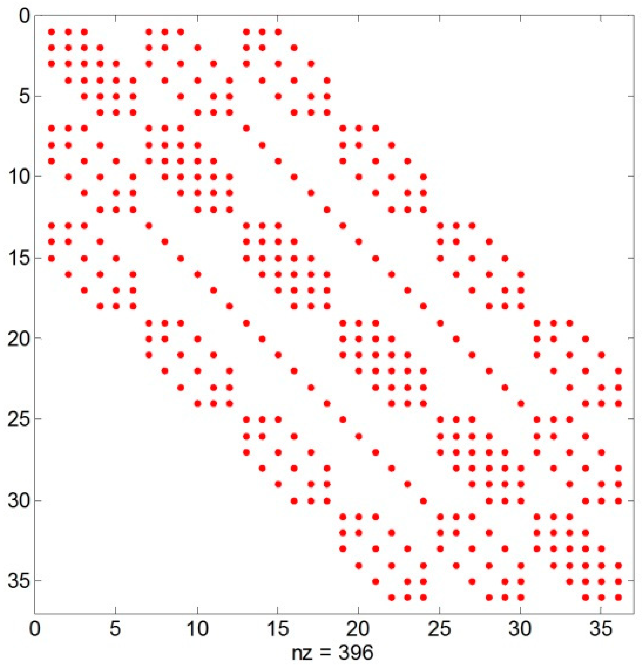
We can see that A is a largely sparse matrix, which has at most 13 nonzero elements for each row (Figure 2), and each element is known beforehand.

4.3. DTM Construction in Practice

Considering the fact that finite difference-based interpolation is only valid in case of gridded data, for the production of DTMs with scattered sample points, the computational domain of the study site must be covered with grid cells, firstly. Then, the points are assigned to the corresponding grids using the following equations:

$$\{\begin{array}{c}i=floor\left(\frac{y-y_{\min }}{h}\right)+1\\ j=floor\left(\frac{x-x_{\min }}{h}\right)+1\end{array}$$

(10)

where (i, j) respectively represent the row and column of the DTM grid cell, which the sample point (x, y) is assigned to; x_min and y_min are the minimum x and y of the sample points; floor(x) is the function that rounds each element of x to the nearest integer less than or equal to that element.

In the process of DTM construction, for solving Equation (9), the general element-wise formula of the Gauss–Seidel method is as follows

$$f_i^{\left(k+1\right)}=\frac{1}{a_{ii}}\left(\frac{w_i}{\lambda }{f}_i^{\left(k\right)}-{\displaystyle \sum _{j=1}^{i-1}{a}_{ij}{f}_j^{\left(k+1\right)}}-{\displaystyle \sum _{j=i+1}^{m\cdot n}{a}_{ij}{f}_j^{\left(k\right)}}\right),i=1,2,\dots ,m\cdot n.$$

(11)

In the computation, when a_ij=0, the corresponding multiplication in the right expression of Equation (11) should be ignored. This can greatly reduce the computational cost due to the large sparseness of A. Theoretically, the Gauss–Seidel method only requires, at most, (13m·n) operations per iteration. Namely, the computational cost of the proposed method is proportional to the total number of grid cells, i.e., O(m·n). Moreover, the Gauss–Seidel-based method does not need the storage of the matrix A. Therefore, the proposed method is extremely fast and has low memory requirement, making it suitable to handle large datasets.

The pseudo codes of the proposed method for DTM generation are shown in Algorithm 1.

Algorithm 1: Proposed method

Input:

P: Sample points P(x, y, z)

λ: Smoothing parameter

I: Number of iterations

h: Desired DTM resolution

Output: A DTM

1. Cover the study domain using grid cells with the resolution of h.

2. For i=1 to size(P).

3.   Assign pi to the grid cell using Equation (10).

4. End.

5. Estimate the values of the unknown grids using nearest neighbor interpolation.

6. For j=1 to I.

8.   For k=1 to size(DTM).

9.      Update the value of the kth grid using Equation (11).

10.   End.

11. End.

5. Experiments

In this section, we respectively employed simulated and real-world LiDAR-derived datasets to assess the performance of the proposed method, and its results were compared with those of some well-known interpolators with respect to interpolation accuracy, computing time, and memory requirement.

5.1. Numerical Test

In the numerical test, we analyzed the results of the proposed method and a recently developed fast TPS method based on DCT [38] for interpolating simulated points. The DCT-based TPS allows fast smoothing and interpolating of data. It was performed with the MATLAB function ‘smoothn’ (https://ww2.mathworks.cn/matlabcentral/fileexchange/25634-robust-spline-smoothing-for-1-d-to-n-d-data?focused=8189808&tab=function). Similar to the proposed method, the initial values of DCT-based TPS were estimated by the nearest neighbor interpolation without other processes. To give a fair comparison, the codes of the new method were also written in MATLAB. The two methods were conducted on a PC with the configuration of Intel^® Core™ i7-4790 CPU @ 3.60 GHz and 16.00 GB RAM.

In the numerical test, we analyzed the results of the proposed method and a recently developed fast TPS method based on DCT [38] for interpolating simulated points. The DCT-based TPS allows fast smoothing and interpolating of data. It was performed with the MATLAB function ‘smoothn’ (https://ww2.mathworks.cn/matlabcentral/fileexchange/25634-robust-spline-smoothing-for-1-d-to-n-d-data?focused=8189808&tab=function). Similar to the proposed method, the initial values of DCT-based TPS were estimated by the nearest neighbor interpolation without other processes. To give a fair comparison, the codes of the new method were also written in MATLAB. The two methods were conducted on a PC with the configuration of Intel^® Core™ i7-4790 CPU @ 3.60 GHz and 16.00 GB RAM.

In the numerical test, we analyzed the results of the proposed method and a recently developed fast TPS method based on DCT [38] for interpolating simulated points. The DCT-based TPS allows fast smoothing and interpolating of data. It was performed with the MATLAB function ‘smoothn’ (https://ww2.mathworks.cn/matlabcentral/fileexchange/25634-robust-spline-smoothing-for-1-d-to-n-d-data?focused=8189808&tab=function). Similar to the proposed method, the initial values of DCT-based TPS were estimated by the nearest neighbor interpolation without other processes. To give a fair comparison, the codes of the new method were also written in MATLAB. The two methods were conducted on a PC with the configuration of Intel^® Core™ i7-4790 CPU @ 3.60 GHz and 16.00 GB RAM.

In the numerical test, we analyzed the results of the proposed method and a recently developed fast TPS method based on DCT [38] for interpolating simulated points. The DCT-based TPS allows fast smoothing and interpolating of data. It was performed with the MATLAB function ‘smoothn’ (https://ww2.mathworks.cn/matlabcentral/fileexchange/25634-robust-spline-smoothing-for-1-d-to-n-d-data?focused=8189808&tab=function). Similar to the proposed method, the initial values of DCT-based TPS were estimated by the nearest neighbor interpolation without other processes. To give a fair comparison, the codes of the new method were also written in MATLAB. The two methods were conducted on a PC with the configuration of Intel^® Core™ i7-4790 CPU @ 3.60 GHz and 16.00 GB RAM.

In the numerical test, we analyzed the results of the proposed method and a recently developed fast TPS method based on DCT [38] for interpolating simulated points. The DCT-based TPS allows fast smoothing and interpolating of data. It was performed with the MATLAB function ‘smoothn’ (https://ww2.mathworks.cn/matlabcentral/fileexchange/25634-robust-spline-smoothing-for-1-d-to-n-d-data?focused=8189808&tab=function). Similar to the proposed method, the initial values of DCT-based TPS were estimated by the nearest neighbor interpolation without other processes. To give a fair comparison, the codes of the new method were also written in MATLAB. The two methods were conducted on a PC with the configuration of Intel^® Core™ i7-4790 CPU @ 3.60 GHz and 16.00 GB RAM.

In principle, the accuracy of DCT-based TPS only depends on the change of the smoothing parameter λ, which is automatically determined by the generalized cross-validation in ‘smoothn’. For the proposed method, its result mainly relies on the number of iterations I and λ. In the test, we set I = 10 based on the tradeoff between interpolation accuracy and efficiency, and λ = 10.

5.1.1. Synthetic Surfaces

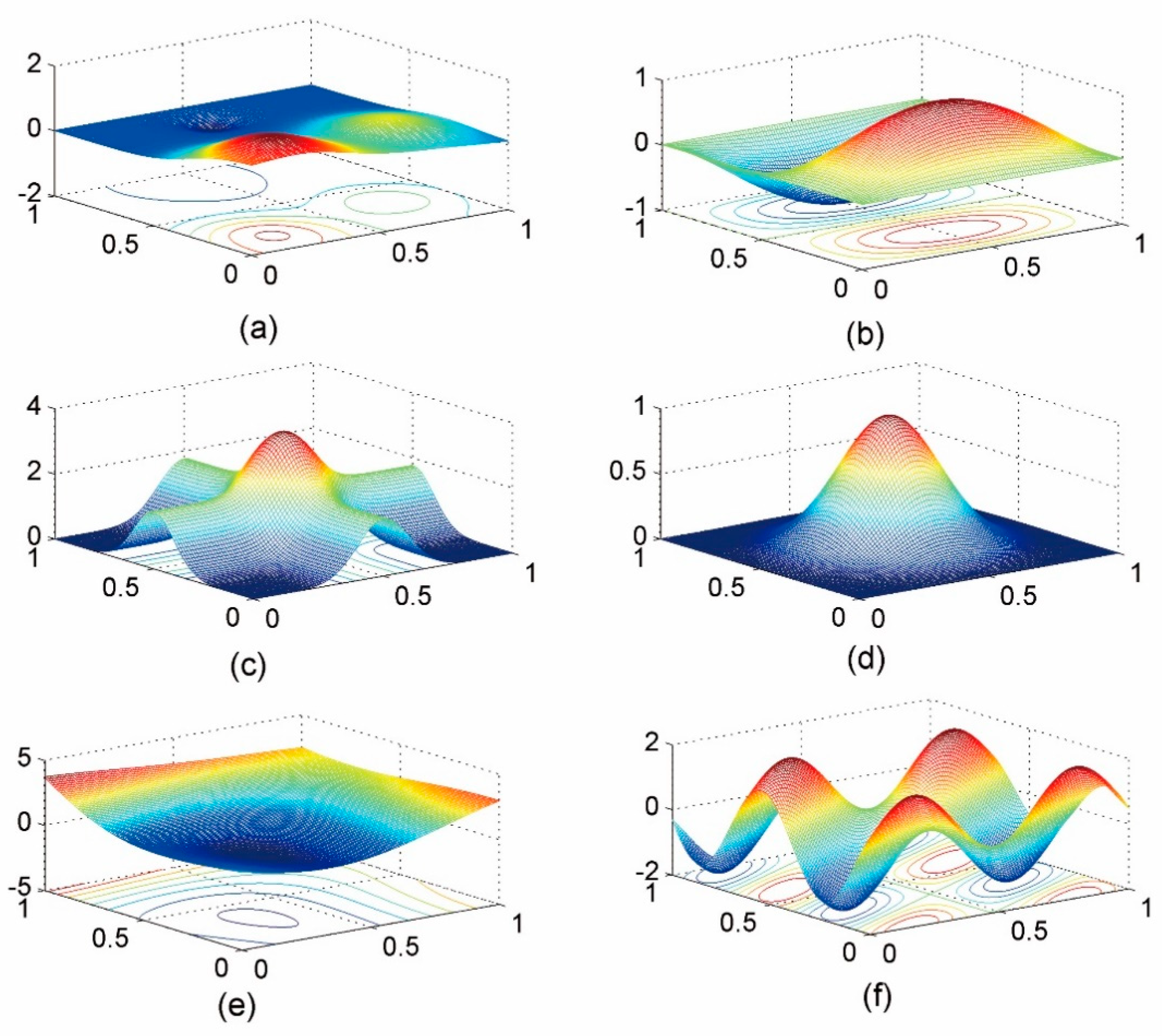
We took six synthetic surfaces as the test surfaces (Figure 3) to assess the efficiency of the proposed method and the DCT-based method. The six surfaces with different shapes are respectively formulated as

$$\begin{array}{cc}\hfill f_1\left(x,y\right)& =\frac{3}{4}{\mathrm{e}}^{-{\left(9x-2\right)}^2/4-{\left(9y-2\right)}^2/4}+\frac{3}{4}{\mathrm{e}}^{-{\left(9x+1\right)}^2/49-{\left(9y+1\right)}^2/10}\hfill \\ & +\frac{1}{2}{\mathrm{e}}^{-{\left(9x-7\right)}^2/4-{\left(9y-3\right)}^2/4}-\frac{1}{5}{\mathrm{e}}^{-{\left(9x-4\right)}^2-{\left(9y-7\right)}^2},\left\{\left(x,y\right)|0\le x,y\le 1\right\}\hfill \end{array}$$

$$f_2\left(x,y\right)=\sin \left(2\pi y\right)\sin \left(\pi x\right),\left\{\left(x,y\right)|0\le x,y\le 1\right\}$$

$$f_3\left(x,y\right)=1.75{\mathrm{e}}^{-{\left(5-10x\right)}^2/2}+1.75{\mathrm{e}}^{-{\left(5-10y\right)}^2/2},\left\{\left(x,y\right)|0\le x,y\le 1\right\}$$

$$f_4\left(x,y\right)=\frac{1}{3}{\mathrm{e}}^{-81\left({\left(x-0.5\right)}^2+{\left(y-0.5\right)}^2\right)/4},\left\{\left(x,y\right)|0\le x,y\le 1\right\}$$

$$\begin{array}{cc}\hfill f_5\left(x,y\right)=& 3{\left(1-x\right)}^2{\mathrm{e}}^{-x^2-{\left(y+1\right)}^2}-10\left(\frac{x}{5}-x^3-y^5\right){\mathrm{e}}^{-x^2-y^2}\hfill \\ & -\frac{1}{3}{\mathrm{e}}^{-{\left(x+1\right)}^2-y^2},\left\{\left(x,y\right)|0\le x,y\le 1\right\}\hfill \end{array}$$

$$f_6\left(x,y\right)=\cos \left(10y\right)+\sin \left(10\left(x-y\right)\right),\left\{\left(x,y\right)|0\le x,y\le 1\right\}.$$

For each surface, 1001×1001 grids were created with an orthogonal division of the computational domain, and 501×501 points were randomly selected by resorting to the so-called Halton sequence, which can generate uniformly distributed random points in [0, l] × [0, l]. Thus, the sample proportion is 25%.

Root mean square error (RMSE) was used to assess the interpolation accuracy. It is formulated as,

$$\mathrm{RMSE}=\sqrt{\frac{{\displaystyle \sum _{i=1}^N{\left(f_i-{\widehat{f}}_i\right)}^2}}{N}}$$

where $f_i$ and ${\widehat{f}}_i$ respectively represent the ith true and simulated values, and N is the number of evaluation points.

5.1.2. Comparative Analysis

The results of the two methods for interpolating the six surfaces are shown in

Table 1. Results of the proposed and DCT-based methods for interpolating the six surfaces.

Surface	Proposed			DCT-Based
	λ	RMSE	Time (s)	λ	RMSE	Time (s)
f1	10	5.95 × 10−4	0.242	11.4	7.39 × 10−4	2.776
f2	10	1.52 × 10−3	0.237	0.52	1.82 × 10−3	3.691
f3	10	2.89 × 10−3	0.241	476.8	3.74 × 10−3	4.493
f4	10	6.93 × 10−4	0.248	301.7	8.83 × 10−4	4.488
f5	10	1.94 × 10−3	0.243	6.6	2.45 × 10−3	2.495
f6	10	3.66 × 10−3	0.247	3.4	3.66 × 10−3	3.759
On average	-	1.883 × 10−3	0.243	-	2.215 × 10−3	3.617

. It is found that the proposed method is always faster and more accurate than the DCT-based method. On average, the former is about 30 times as fast as the latter. The high speed of the proposed method owes to the fact that the nonzero elements of the interpolation matrix are known beforehand, and the Gauss–Seidel method makes full use of the sparseness of the matrix. The DCT-based method requires different smoothing parameter for interpolating the six surfaces. This indicates its high sensitivity to the smoothing parameter. Compared to the proposed method, the slightly lower accuracy of the DCT method might be due to the sub-optimal smoothing parameter determined by the generalized cross-validation.

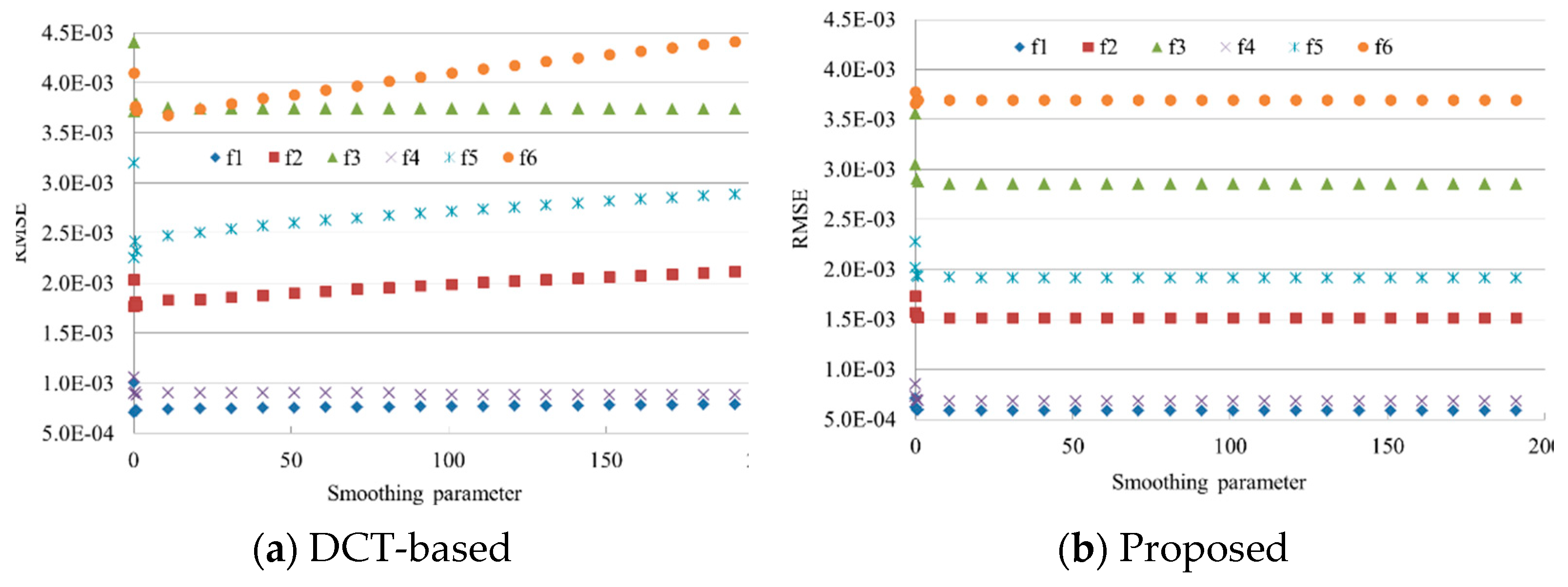
We assess the influence of the smoothing parameter λ on the results of the two methods, since it has an effect on the interpolation accuracy. We set $\lambda =\left\{0.01,0.1,0.5,1:10:200\right\}$ for the two methods, and the number of iterations is 15 for the proposed method. Results (Figure 4a) demonstrate that with the increase of λ, the RMSEs of the DCT-based method become larger on three surfaces, i.e., f₂, f₅, and f₆. These surfaces seem more complex than the others (Figure 3). The DCT method has the best performance on λ = 0.01 for the three surfaces, which is completely different from the values derived from the generalized cross-validation method (Table 1). This further indicates its unreliability, caused by the fact that the generalized cross-validation is based on the assumption of the independence of the sample points [39]. In comparison, the proposed method (Figure 4b) is less sensitive to the smoothing parameter when it is larger than 10. This is very helpful in practice as it is tedious and time-consuming for determining the optimal parameter. Regardless of the smoothing parameter, the proposed method always outperforms the DCT-based method.

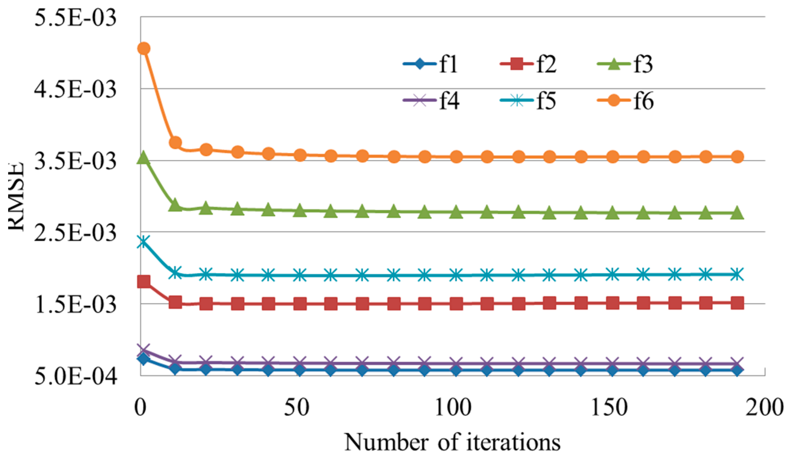
Since the number of iterations I influence the convergence, we further assess its effect on the result of the proposed method. Here, we set λ = 10 and $I=\left\{1:10:200\right\}$. We can see that when I is larger than 10, the result seems stable on all synthetic surfaces (Figure 5). This proves the high rate of convergence of the proposed method.

The random-access memory requirements of the two methods mainly depend on the number of sample points and grid cells, unrelated to the shape of the synthetic surfaces. Thus, taking f₁ as an example, we compute their memory costs. We found that the DCT-based and the proposed method need the memory costs of about 87.2 M and 29.5 M, respectively. Namely, the memory cost of the former is about three times as large as that of the latter. The large cost of the DCT-based method is mainly due to the storage of DCT and inverse DCT matrices, weight matrix, and the eigenvalues of the finite difference operators.

5.2. Real-World Applications

In the real-world examples, the effects of topographic variability and sampling density on the performance of the proposed method for DTM generation were assessed using 10 public and 1 private LiDAR-derived datasets. In principle, the existing interpolation methods can be roughly categorized into two groups: Locally weighted interpolation and global finite difference interpolation. Inverse distance weighting (IDW), ordinary kriging (OK), natural neighbor (NN), and linear interpolation based on a Delaunay triangulation belong to the former, while the DCT-based TPS and the proposed method belong to the latter. In addition to the DCT-based TPS, the locally weighted interpolators were also used for comparison. The general formula for these interpolators is formulated as

$$z\left({\mathit{x}}_0\right)={\displaystyle \sum _{i=1}^N{w}_{i}z\left({\mathit{x}}_i\right)}$$

(12)

where $z\left({\mathit{x}}_i\right)$ and w_i are the value and weight of the ith sample point, respectively; ${\mathit{x}}_0\in R^2$ is the point to be predicted; and N is the number of sample points used for computation. Equation (12) indicates that the local interpolation methods weight the surrounding measured values to derive a prediction for an unmeasured location, and the main difference between the interpolators is the way to determine the weight w.

Prior to DTM grid value estimation using Equation (12), some preliminary operations should be conducted for the local interpolators, namely the linear and NN method should construct Delaunay triangulation, IDW should search the k nearest neighbors, and OK needs to estimate the weights by sequentially computing the experimental variogram, fitting a theoretical variogram to the experimental one, and solving a dense linear system. In this paper, we used the kd-tree algorithm to search the k nearest neighbors [40] and the divide and conquer algorithm for Delaunay triangulations [41]; both time complexities are O(N·logN) and space complexities are O(N). The time and memory costs of OK for estimating weights are O(N³) and O(N²), respectively, since it must solve a dense linear system. For all the local interpolation methods, DTM construction with Equation (12) requires O(n) time complexity, where n is the number of DTM grids.

Based on the aforementioned discussion,

Table 2. Time complexities of the proposed method and the classical interpolation methods for Dconstruction.

Method	Search k Nearest Neighbors	Construct Delaunay Triangulations	Estimate Weights	Estimate Grid Values
Proposed	-	-	-	O(n)
Linear	-	O(N·logN)	-	O(n)
NN	-	O(N·logN)	-	O(n)
IDW	O(N·logN)	-	-	O(n)
OK	O(N·logN)	-	O(N3)	O(n)

and

Table 3. Space complexities of the proposed method and the classical interpolation methods for DTM construction.

Method	Sample Points	Delaunay Triangulations/KD-Tree	Weight Estimation	DTM
Proposed	O(N)	-	-	O(n)
Linear	O(N)	O(N)	-	O(n)
NN	O(N)	O(N)	-	O(n)
IDW	O(N)	O(N)	-	O(n)
OK	O(N)	O(N)	O(N2)	O(n)

, respectively, show the time and space complexities of all the interpolation methods for each step during DTM generation. Theoretically, the proposed method seems to have less memory and computational costs than the other methods.

In the test, for OK, we employed the existing ‘kriging’ function (https://cn.mathworks.com/matlabcentral/fileexchange/29025-ordinary-kriging) to perform interpolation, where the computation of the experimental variogram and the fit of a theoretical variogram to the experimental one were, respectively, conducted with the functions of ‘variogram’ (https://cn.mathworks.com/matlabcentral/fileexchange/20355-experimental--semi---variogram) and ‘variogramfit’ (https://cn.mathworks.com/matlabcentral/fileexchange/25948-variogramfit). Since variogram fitting is computationally expensive, only 5000 points, randomly selected from the training dataset, were used to fit the variogram. Note that all the interpolation methods were executed in MATLAB.

In the process of parameter determination, we tested different combinations. Specifically, the number of neighbors ranges from 15 to 40 with the step of 5 for IDW and OK. The power value of IDW varies from 1 to 5 with the step of 1. The smoothing parameters of the proposed method and the DCT-based TPS are $\lambda =\left\{{10}^{-4},{10}^{-3},{10}^{-2},0.1,1,5,10\right\}$, and the number of iterations of the proposed method is 20. Moreover, the smoothing parameter of the DCT-based method was also determined by the generalized cross-validation. Hereafter, for ease of discussion, DCT-based TPS with the parameter determined by trial-and-error and generalized cross-validation were termed DCT-T and DCT-G, respectively. NN and the linear interpolation do not require any parameters.

5.2.1. Public Dataset

Ten benchmark datasets with different terrain characteristics, provided by the International Society for Photogrammetry and Remote Sensing (ISPRS) Commission III [42], were used to analyze the interpolation accuracy of the proposed method. Since the point labels (i.e., ground or nonground) in the dataset were known beforehand, only the ground points were used to produce DTMs. Firstly, the ground points were randomly divided into training and testing points consisting of 90% and 10% of points, respectively, then the former was used to produce DTMs and the latter to assess the DTM accuracy.

Table 4. Data description for each sample.

Sample	#Training	#Testing	Area (ha)	Point Space (m)	STD (m)	Cell Size (m)
s-11	19,607	2179	4.05	0.69	29.2	0.5
s-12	24,021	2670	5.40	0.68	3.1	0.5
s-21	9076	1009	1.43	0.63	0.6	0.5
s-22	20,253	2251	3.40	0.64	2.8	0.5
s-31	14,000	1556	2.82	0.75	0.9	0.5
s-41	5041	561	1.75	0.51	3.5	0.25
s-51	12,555	1395	9.99	1.72	15.1	1
s-52	18,100	2012	13.55	1.74	28.8	1
s-61	30,468	3386	22.39	1.55	7.1	1
s-71	12,487	1388	8.73	1.72	3.0	1

gives the numbers of training points (#training) and testing points (#testing), area, and average point space for each sample. In addition, the standard deviation (STD) of elevations for describing terrain characteristic was also provided. Results exhibit that the 10 samples with different areas have various terrain complexities. Hengl [43] indicated that a signal can be reconstructed if the sampling frequency is twice that of the original frequency. Thus, a cell size that keeps the majority of the information inherent in the original point dataset should be half the average point space between the closest point pairs. In addition, cell sizes of 0.25 m, 0.5 m, or 1.0 m are commonly used for lidar-derived DTMs in practice. Thus, based on the theory and practice, the optimal cell size for each sample is given in Table 4.

Interpolation results (Figure 6) show that terrain characteristics have a significant effect on the interpolation accuracy. Specifically, regardless of interpolators, s-21 and s-31, which are less complex than the other samples, have higher accuracy, while s-11 with the greatest complexity obtains the lowest accuracy. Among the interpolation methods, DCT-G tends to produce the poorest results in almost all samples, except for s-41. DCT-T always yields better results than DCT-G. This indicates that the generalized cross-validation method is unreliable for the determination of the smoothing parameter in practice. OK performs best in 9 out of 10 samples, and the proposed method is approximately as accurate as OK.

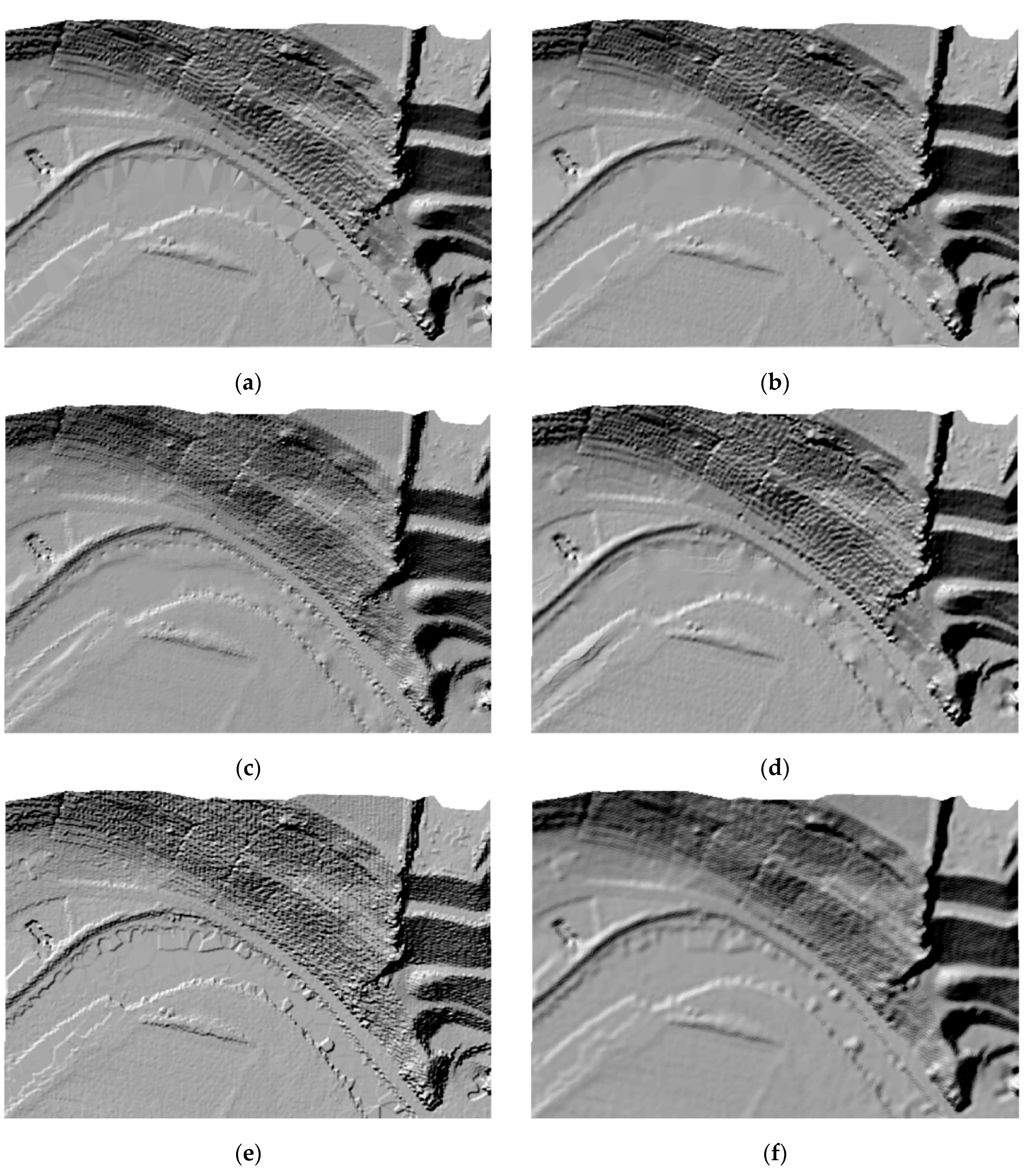
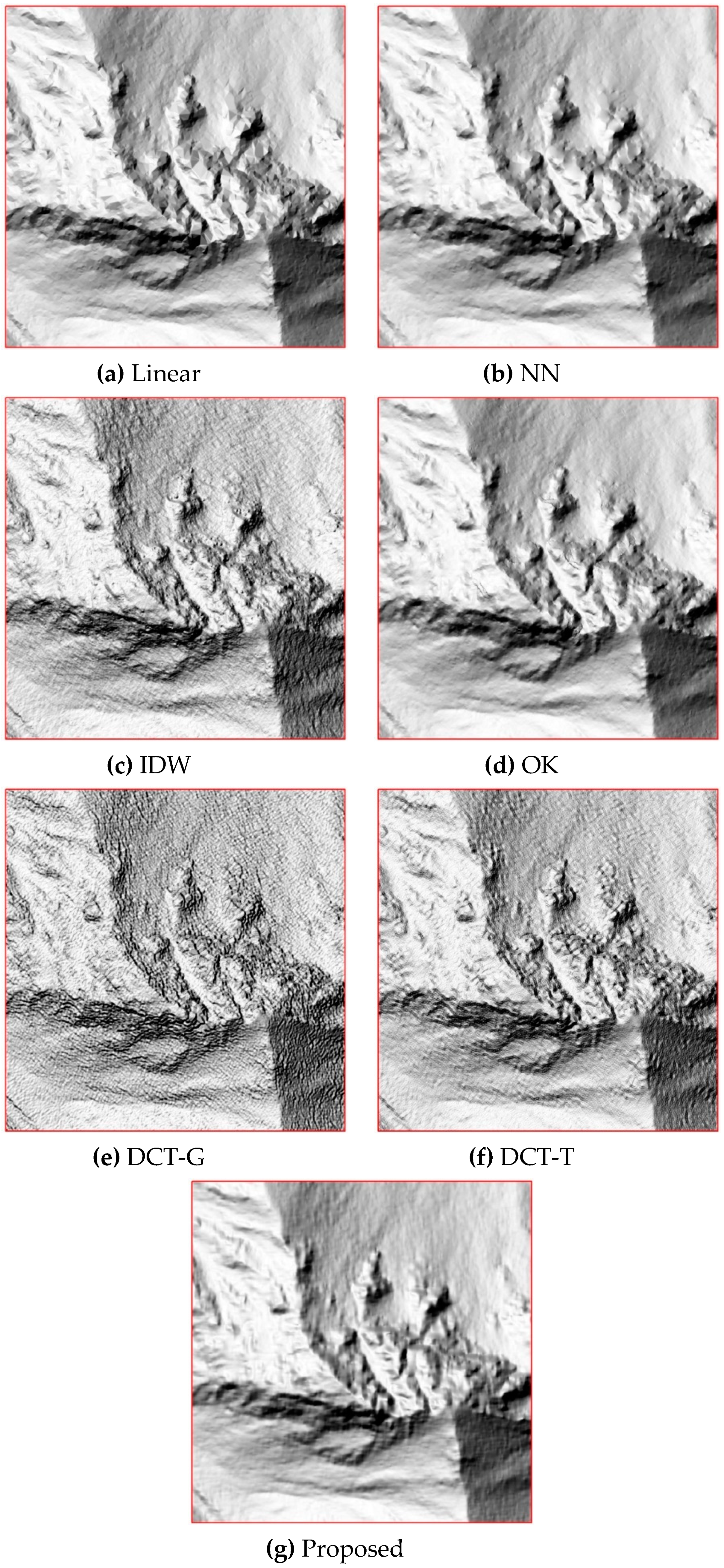
S-52 is taken as a representative to visually show the interpolated surfaces of all the methods, as this sample is characterized by a complex landscape including flat terrain, steep slopes, and break lines. Shaded relief maps show that the linear interpolation produces faceted surfaces where the sample density is low (Figure 7a). This is because the linear method cannot handle complex terrain with nonlinear features. NN has sporadic outliers in the steep slopes due to its exact interpolation nature (Figure 7b). IDW suffers from strips and pits in areas of steep slopes and flat areas (Figure 7c). OK seems to generate a smooth surface, yet it has tree root-like discontinuities in the flat area because of its local interpolation nature (Figure 7d). DCT-G has many bumps in the flat area and generates coarse surfaces in the steep slopes (Figure 7e). The bumps of the DCT-G disappear in the surface of DCT-T, yet the steep slopes of the latter are blurred (Figure 7f). The poor performance of the two DCT-based TPSs may be caused by their high sensitivity to the smoothing parameter, whose value was not optimally tuned. The proposed algorithm produces the most visually appealing surface, which is generally smooth and free of obvious artifacts (Figure 7g). The good performance of the proposed method is thanks to the global interpolation manner and insensitivity to the smoothing parameter.

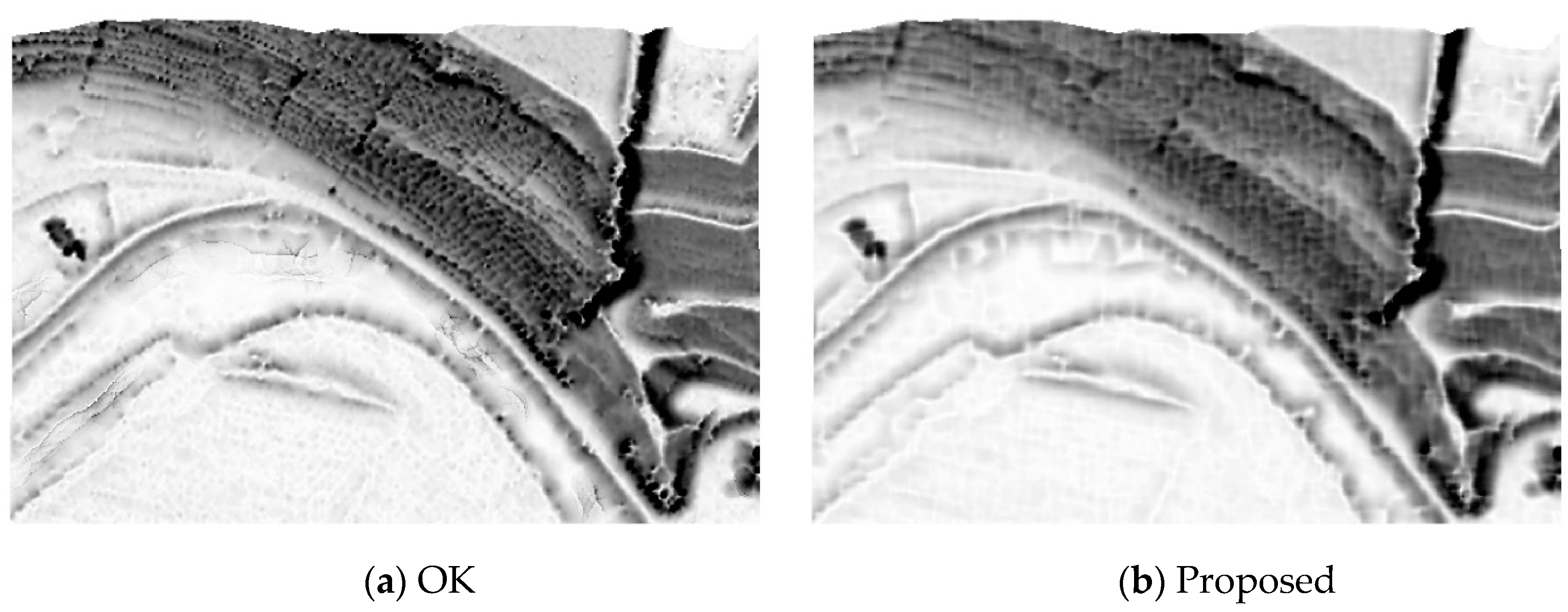
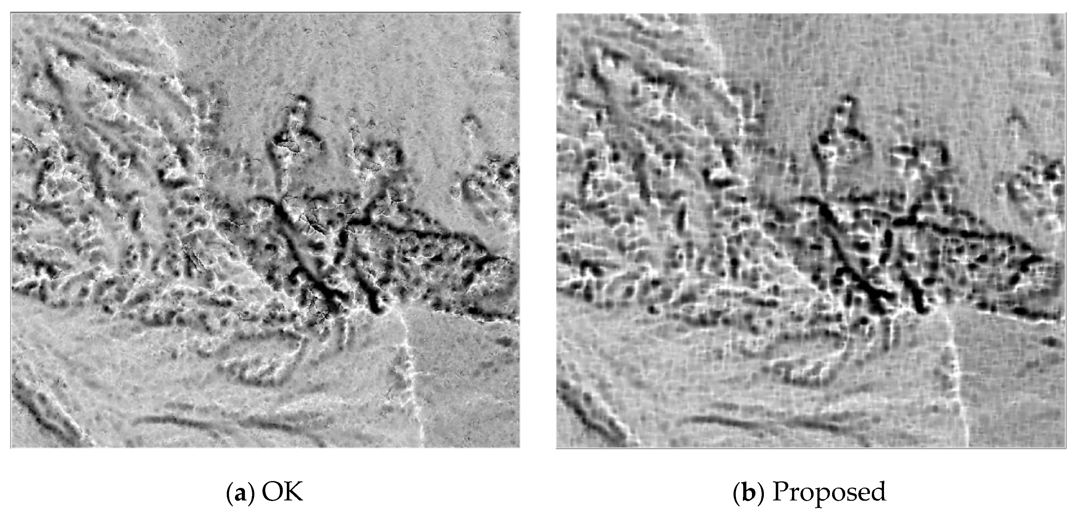
Although shaded relief map is a widely accepted technique for visually showing DTMs, it has two major drawbacks: Identifying details in deep shades and inability to properly represent linear features lying parallel to the light beam. In comparison, sky-view factor can be used as a general relief visualization technique to show relief characteristics [44,45]. Thus, the sky-view factors of OK and the proposed method on s-52 are demonstrated in Figure 8. They are produced with Relief visualization Toolbox (https://www.zrc-sazu.si/en/rvt). Obviously, OK surfers from tree-like discontinuities in the flat terrain (Figure 8a), which is inconspicuous in the shaded relief map (Figure 7d). However, these discontinuity features are avoided by the proposed method (Figure 8b).

The rasterization time of all the methods on the 10 samples are shown in

Table 5. Rasterization time (reading the points, interpolation, and writing on disk) of the proposed method and the other interpolation methods on the public datasets (unit: s).

Sample	Linear	NN	IDW	OK	DCT-Based	Proposed
s-11	4.29	4.91	5.46	333.80	4.03	3.90
s-12	5.96	6.84	7.61	582.99	5.25	5.30
s-21	1.77	1.95	2.22	99.73	1.57	1.58
s-22	4.22	4.75	5.41	300.16	3.76	3.77
s-31	2.54	2.85	3.16	156.01	2.21	2.21
s-41	3.24	4.00	4.25	200.28	2.94	2.89
s-51	1.76	1.94	2.18	150.00	1.55	1.53
s-52	2.33	2.57	2.90	154.47	2.08	2.03
s-61	4.76	5.44	6.03	313.18	4.19	4.18
s-71	1.69	1.83	2.07	86.99	1.59	1.36
On average	3.26	3.71	4.13	237.76	2.92	2.88

. The time includes the costs for reading sample points, DTM interpolation, and storage transfer from random-access memory to the disk. Results demonstrate that irrespective of samples, the OK method has the largest computational time. Linear interpolation and NN are slightly faster than IDW since the former do not require the search of neighbors. In comparison, the proposed and the DCT-based methods are faster than the other methods. On average, the proposed method has the highest speed and is about 83 times as fast as OK. Note that compared to the DCT-based method, the efficiency of the proposed method is less obvious on the real-world dataset than on the simulated one. This is because saving DTMs from the random-access memory to the disk is much more time-consuming than solving the linear system of TPS.

Random access memory costs of all the methods on the samples are shown in

Table 6. Random access memory costs of the proposed method and the other interpolation methods on the public datasets (unit: M).

Sample	Linear	NN	IDW	OK	DCT-T	Proposed
s-11	3.52	3.52	33.69	441.49	6.38	1.76
s-12	4.80	4.80	47.47	446.92	8.42	2.26
s-21	1.52	1.52	14.20	398.23	2.34	0.70
s-22	3.57	3.57	33.93	468.70	5.51	1.62
s-31	2.21	2.21	20.03	384.79	4.46	1.25
s-41	2.24	2.24	25.95	425.83	2.61	0.62
s-51	1.67	1.67	13.97	386.10	14.28	2.91
s-52	2.29	2.29	18.59	381.84	19.43	3.99
s-61	4.36	4.36	37.87	462.90	32.07	6.61
s-71	1.54	1.54	12.30	406.57	12.54	2.61
On average	2.77	2.77	25.80	420.34	10.80	2.43

. Irrespective of the sample, the proposed method always has the least memory requirement, and OK has the largest. On average, the cost of the proposed method is about 1.14, 1.14, 10.62, 172.98, and 4.44 times less than those of the linear, NN, IDW, OK, and DCT-based methods, respectively.

5.2.2. Private Dataset

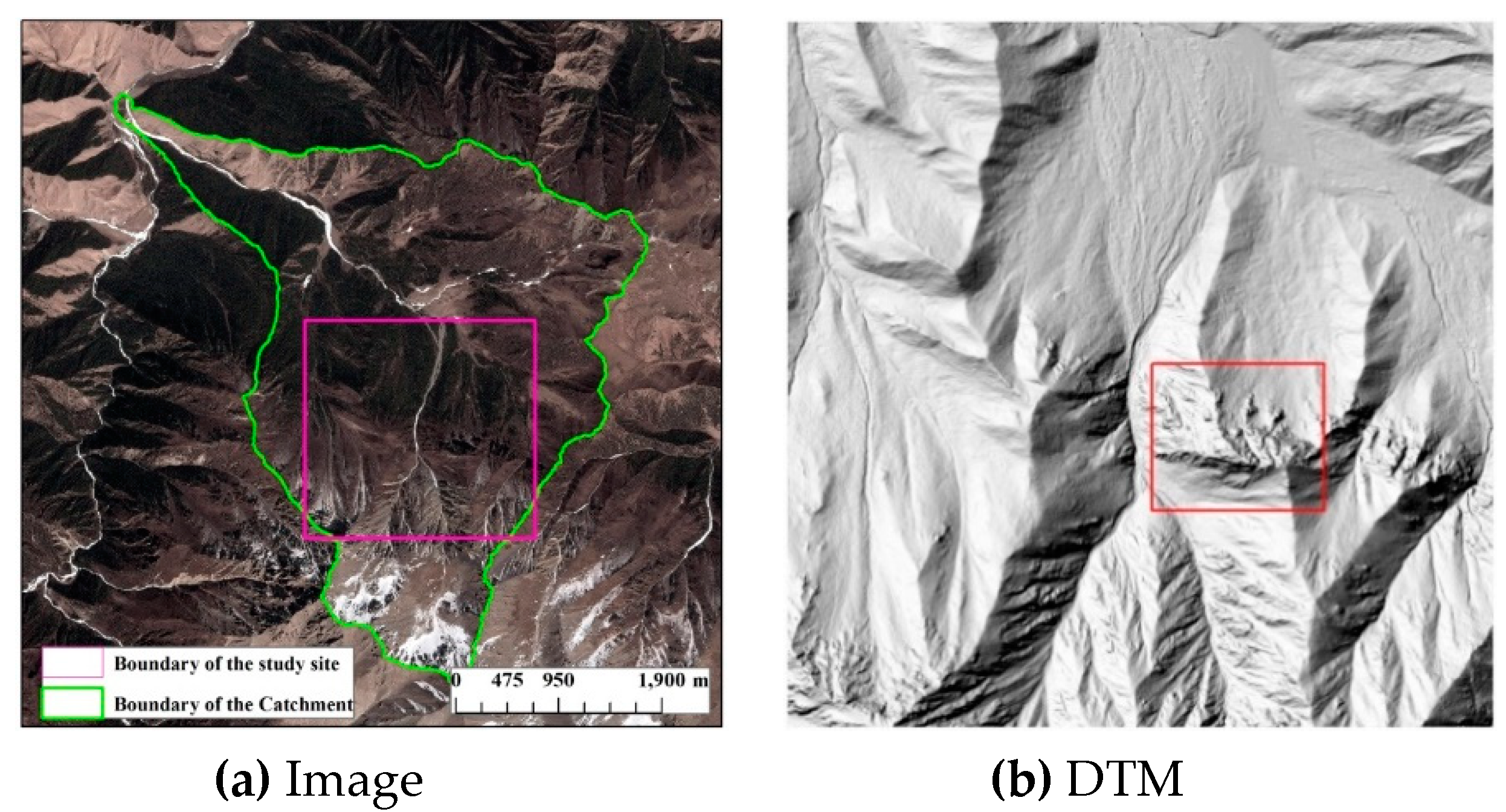
The study site is mainly located in Tianlaochi Catchment, Gansu province, China (Figure 9). It covers an area of 2100 × 2100 m² with the mean elevation and the standard deviation of 3353.8 m and 239.4 m, respectively. Raw LiDAR data in the study site was captured using Leica ALS70 with the laser wavelength of 1064 nm and absolute flying height of 4800 m in July 2012. TerraScan, one of the main applications in the Terrasolid Software, was used to automatically filter the raw LiDAR point cloud. Then, the filtered points were manually edited with the help of orthoimages to assure the filtering accuracy. After that, 2,090,337 ground points and 4,189,499 nonground points were obtained. Like the process for handling the public dataset, 90% and 10% of ground points were, respectively, used as the training and testing data. The average point space of the training points is about 1.5 m. Thus, the desired DTM resolution should be 0.75 m. In addition to interpolation methods, sample density also has a significant influence on DTM accuracy [7]. Thus, we used different proportions of training samples to generate DTMs, namely 100%, 80%, 60%, 30%, and 10%.

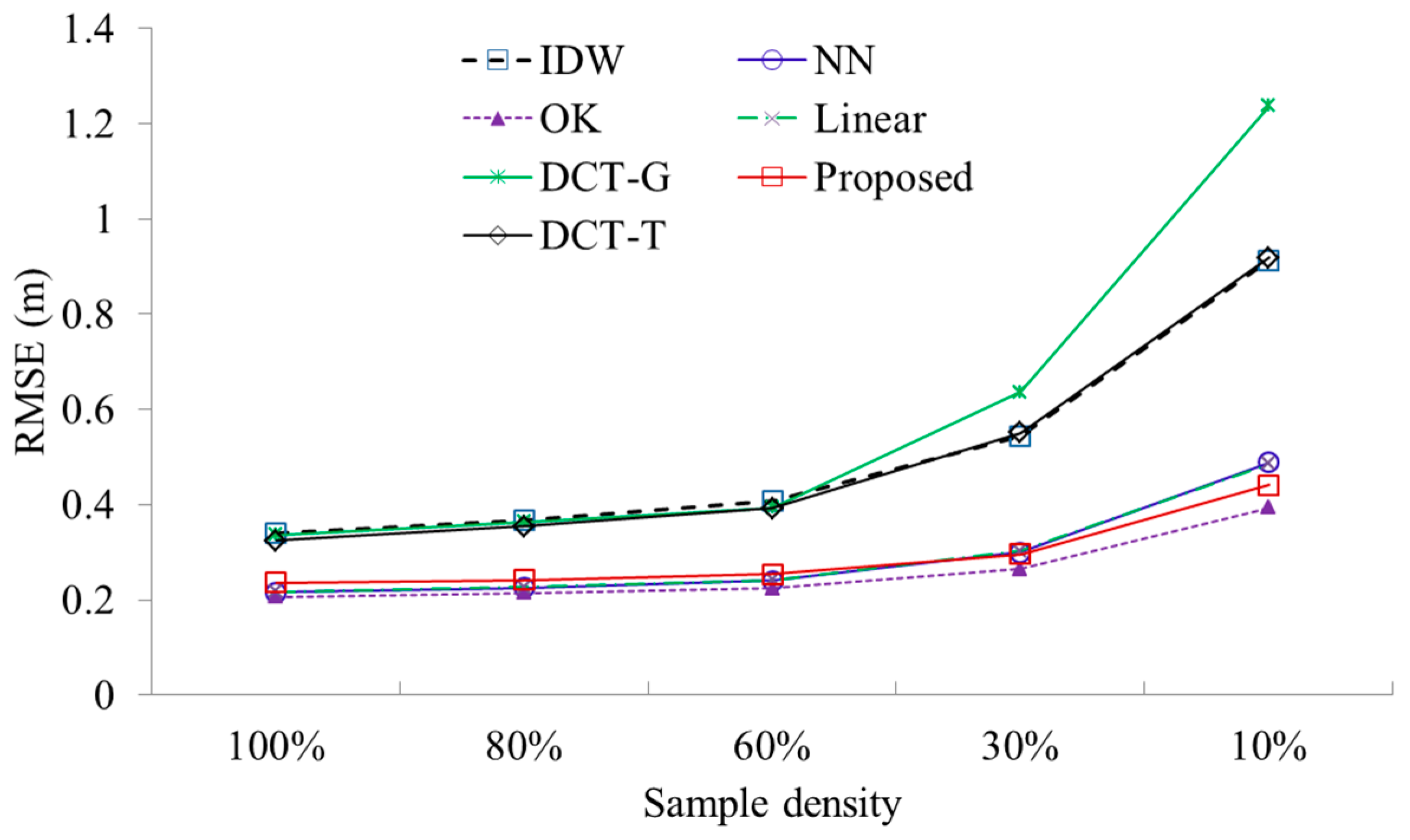
Results (Figure 10) demonstrated that as sample density decreases, the accuracies of all methods become lower. This conclusion is apparent as lower sample density means less captured terrain information. Regardless of sample density, OK consistently ranks the first, which is closely followed by the proposed method, linear, and NN. DCT-G always ranks the last. Although DCT-T performs slightly better than DCT-G, the former has much lower accuracy than the proposed method. This indicates that DCT is less reliable than the Gauss–Seidel method for solving the linear system of TPS in the real-world applications.

Figure 11 shows the shaded relief maps of all the interpolation methods on the 30% of training points in the area denoted by the red rectangle in Figure 9b. We can see that linear interpolation (Figure 11a) and NN (Figure 11b) have obvious peak-cutting problems in the ridges. This result is mainly due to the fact that the two methods cannot estimate peaks or valleys that occur beyond the elevation range limits of a given same dataset [10]. IDW produces a coarse surface because it is an exact interpolator (Figure 11c). It seems that OK generates a smooth surface, yet it suffers from discontinuities in some ridges because of the local interpolation nature (Figure 11d). This is clearly demonstrated with its positive openness map (Figure 12a), which was also produced with the Relief visualization Toolbox (https://www.zrc-sazu.si/en/rvt). The two versions of DCT-based methods generate very coarse surfaces, caused by their sensitivity to the smoothing parameter and its improper estimation (Figure 11e,f). In comparison, the proposed method obtains the most visually pleasing surface, where the terrain features are accurately preserved and the noise is smoothed out (Figure 11g). In addition, compared to OK, the discontinuity features cannot be found in the positive openness map of the proposed method (Figure 12b), which is mainly attributed to its global interpolation manner.

The computational costs (

Table 7. Rasterization time (reading the points, interpolation, and writing on disk) of the proposed method and the other interpolation methods on the private dataset (unit: s).

Data Proportion	Linear	NN	IDW	OK	DCT-Based	Proposed
100%	118.2	133.0	200.5	2555.4	96.7	94.7
80%	124.3	135.6	314.7	2675.1	98.1	93.5
60%	110.7	123.4	322.9	2659.6	92.1	91.0
30%	105.1	115.7	216.0	2553.5	91.6	95.7
10%	100.6	111.8	143.9	2479.7	90.7	91.0
On average	111.8	123.9	239.6	2584.7	93.8	93.2

) show that OK is extremely more time-consuming than the other methods. The proposed and DCT-based methods have faster speeds, which are closely followed by linear, NN, and IDW. These conclusions are consistent with that from the public dataset of this paper.

Table 8. Random-access memory costs of the proposed method and the other interpolation methods on the private dataset (unit: G).

Data Proportion	Linear	NN	IDW	OK	DCT-T	Proposed
100%	0.14	0.14	0.83	2.35	0.66	0.17
80%	0.13	0.13	0.82	2.33	0.65	0.16
60%	0.11	0.11	0.80	2.32	0.63	0.14
30%	0.08	0.08	0.78	2.30	0.61	0.12
10%	0.07	0.07	0.77	2.28	0.60	0.11
On average	0.11	0.11	0.80	2.32	0.63	0.14

shows the random-access memory costs of all the interpolation methods. Results indicate that regardless of data proportion, the proposed method has similar memory costs to linear and NN, and less than IDW and DCT-T. OK has the largest costs, which is 2.32 G on average. It is about 16.6 times as large as that of the proposed method.

6. Discussion and Conclusions

6.1. Discussion

Nowadays, airborne LiDAR has been gaining recognition as an effective tool for the derivation of DTMs in Earth science, where interpolation is an indispensable process. Because of the high-density and high-accuracy of LiDAR datasets, some researchers indicated that simple interpolation methods, such as natural neighbor (NN), linear, and inverse distance weighting (IDW), are more useful. For example, Abramov and McEwen [46] concluded that NN was not only the most accurate algorithm, but also generated the fewest visual artifacts. Su and Bork [47] found that IDW is the most accurate interpolator. Bater and Coops [8] indicated that NN provided the best result with a minimum of effort. Guo et al. [7] regarded that simple interpolation methods are more efficient for generating DTMs from LiDAR data. Razak et al. [48] found that IDW was favored because it combined computational times more reasonably without adding artifacts to the DTM. Montealegre et al. [3] showed that linear interpolation produced the best result in the validation process with the training dataset while IDW was the best in the validation with GPS. However, our results on the 10 public and 1 private datasets indicate that although the simple interpolation methods can obtain relatively low RMSEs with less computational costs, they suffer from visual interpolation artifacts, such as the peak-cutting problem of linear and NN, and the dimpled and coarse surface of IDW.

Some scholars highly recommended kriging for the derivation of DTMs from LiDAR datasets. For example, Lloyd and Atkinson [49] found that kriging was the most accurate method when sample density was low. Guo et al. [7] indicated that OK was more reliable if accuracy was the most important consideration. Chu et al. [6] demonstrated that for sparse samples in the forest, landslide scarp identification based on kriging-estimated DTM was more faithful. However, our results exhibit that despite the high interpolation accuracy, kriging has a huge computational cost. Moreover, kriging with a local support is prone to the creation of discontinuous DTMs, which was also concluded by Meyer [36]. By contrast, our proposed method produces visually pleasing surfaces, which are smooth and free of interpolation artifacts. More importantly, the new method compares favorably with the simple linear interpolation methods with respect to computing cost and random-access memory requirement and is extremely faster than OK.

Recently, a regularized method was proposed to deal with the ill-conditioning problem of thin plate spline (TPS) on the noisy sample points [50]. Compared to the classical TPS, the accuracy of the regularized-based method is improved. However, it suffers from huge computing costs when interpolating large datasets, which greatly hinders its widespread applications. To improve the computing efficiency of TPS interpolation in the process of filtering point clouds, the DCT-based method [38] is employed to solve the linear system of finite difference TPS [18]. However, as demonstrated in this paper, the DCT-based method has worse performance than the proposed method in terms of computing cost, memory requirement, and interpolation accuracy. Moreover, the former is highly sensitive to the smoothing parameter in practice. Therefore, we strongly suggest the replacement of the DCT-based method with the newly developed method for reference ground surface generation.

6.2. Conclusions

To efficiently generate high-quality DTMs from large LiDAR-derived datasets, we propose a fast, global interpolation method in this paper. The proposed method uses a weighted thin plate spline (TPS) to overcome the problem of missing data in the grid-based surface generation. Moreover, to decrease the computational requirement with respect to memory and time costs, the interpolation matrix of the weighted TPS is deduced, and the values and positions of all the nonzero elements of the matrix are analytically obtained. Afterwards, the linear system is efficiently solved by making full use of matrix sparseness. Numerical tests indicate that the proposed method has higher accuracy, and lower computing and memory costs than the recently developed DCT-based method. Furthermore, the proposed method is insensitive to the smoothing parameter, which is very useful and helpful in practice. Tests on 11 real-world LiDAR datasets show that compared to some well-known locally weighted interpolators and the DCT-based TPS, the proposed method can produce visually pleasing surfaces without interpolation artifacts. More importantly, the computing and memory costs of the new method are comparable to those of the simple interpolation methods, like IDW and NN, and are much lower than those of OK.

However, the proposed method also has some limitations. Since the proposed method works on the grid-based surface, spatial location errors are unavoidable when large-resolution surfaces are to be interpolated. Moreover, because the proposed method requires an iterative computation, at least 10 iterations should be used to assure the convergence of the results, thereby increasing computational costs. Hence, one of our further works will focus on the improvement of interpolation accuracy and convergence rate to make the method more practical. Since the proposed method with the effect of smoothness seems suitable for the production of smooth DTMs, it is helpful for the applications, such as analysis of flood prone areas or drainage networks. Hence, to test how well it suits for these applications is of also paramount importance.

References

- Liu, X.; Zhang, Z. Effects of LiDAR data reduction and breaklines on the accuracy of digital elevation model. Surv. Rev. 2011, 43, 614–628. [Google Scholar] [CrossRef]
- Yang, B.; Huang, R.; Dong, Z.; Zang, Y.; Li, J. Two-step adaptive extraction method for ground points and breaklines from lidar point clouds. ISPRS J. Photogramm. Remote Sens. 2016, 119, 373–389. [Google Scholar] [CrossRef]
- Montealegre, A.; Lamelas, M.; Riva, J. Interpolation routines assessment in ALS-derived digital elevation models for forestry applications. Remote Sens. 2015, 7, 8631–8654. [Google Scholar] [CrossRef]
- Tarolli, P. High-resolution topography for understanding Earth surface processes: Opportunities and challenges. Geomorphology 2014, 216, 295–312. [Google Scholar] [CrossRef]
- Shi, W.; Zheng, S.; Tian, Y. Adaptive mapped least squares SVM-based smooth fitting method for DSM generation of LIDAR data. Int. J. Remote Sens. 2009, 30, 5669–5683. [Google Scholar] [CrossRef]
- Chu, H.; Wang, C.; Huang, M.; Lee, C.; Liu, C.; Lin, C. Effect of point density and interpolation of LiDAR-derived high-resolution DEMs on landscape scarp identification. GISci. Remote. Sens. 2014, 51, 731–747. [Google Scholar] [CrossRef]
- Guo, Q.; Li, W.; Yu, H.; Alvarez, O. Effects of topographic variability and Lidar sampling density on several DEM interpolation methods. Photogramm. Eng. Remote Sens. 2010, 76, 701–712. [Google Scholar] [CrossRef]
- Bater, C.W.; Coops, N.C. Evaluating error associated with lidar-derived DEM interpolation. Comput. Geosci. 2009, 35, 289–300. [Google Scholar] [CrossRef]
- Hutchinson, M.F.; Gessler, P.E. Splines—More than just a smooth interpolator. Geoderma 1994, 62, 45–67. [Google Scholar] [CrossRef]
- Doucette, P.; Beard, K. Exploring the capability of some GIS surface interpolators for DEM gap fill. Photogramm. Eng. Remote Sens. 2000, 66, 881–888. [Google Scholar]
- Desmet, P.J.J. Effects of interpolation errors on the analysis of DEMs. Earth Surf. Process. Landf. 1998, 22, 563–580. [Google Scholar] [CrossRef]
- Erdogan, S. A comparison of interpolation methods for producing digital elevation models at the field scale. Earth Surf. Processes Landforms 2009, 34, 366–376. [Google Scholar] [CrossRef]
- Mongus, D.; Zalik, B. Parameter-free ground filtering of LiDAR data for automatic DTM generation. ISPRS J. Photogramm. Remote Sens. 2012, 67, 1–12. [Google Scholar] [CrossRef]
- Evans, J.S.; Hudak, A.T. A multiscale curvature algorithm for classifying discrete return lidar in forested environments. IEEE Trans. Geosci. Remote Sens. 2007, 45, 1029–1038. [Google Scholar] [CrossRef]
- Hu, H.; Ding, Y.; Zhu, Q.; Wu, B.; Lin, H.; Du, Z.; Zhang, Y.; Zhang, Y. An adaptive surface filter for airborne laser scanning point clouds by means of regularization and bending energy. ISPRS J. Photogramm. Remote Sens. 2014, 92, 98–111. [Google Scholar] [CrossRef]
- Chen, C.; Li, Y.; Yan, C.; Dai, H.; Liu, G.; Guo, J. An improved multi-resolution hierarchical classification method based on robust segmentation for filtering ALS point clouds. Int. J. Remote Sens. 2016, 37, 950–968. [Google Scholar] [CrossRef]
- Chen, C.F.; Li, Y.Y.; Li, W.; Dai, H.L. A multiresolution hierarchical classification algorithm for filtering airborne LiDAR data. ISPRS J. Photogramm. Remote Sens. 2013, 82, 1–9. [Google Scholar] [CrossRef]
- Chen, C.F.; Li, Y.Y.; Zhao, N.; Guo, J.Y.; Liu, G.L. A fast and robust interpolation filter for airborne lidar point clouds. PLoS ONE 2017, 12, e0176954. [Google Scholar] [CrossRef] [PubMed]
- Buckley, M.J. Fast computation of a discretized thin-plate smoothing spline for image data. Biometrika 1994, 81, 247–258. [Google Scholar] [CrossRef]
- Beatson, R.K.; Cherrie, J.B.; Mouat, C.T. Fast fitting of radial basis functions: Methods based on preconditioned GMRES iteration. Adv. Comput. Math. 1999, 11, 253–270. [Google Scholar] [CrossRef]
- Ling, L.; Kansa, E.J. A least-squares preconditioner for radial basis functions collocation methods. Adv. Comput. Math. 2005, 23, 31–54. [Google Scholar] [CrossRef]
- Faul, A.C.; Goodsell, G.; Powell, M.J.D. A Krylov subspace algorithm for multiquadric interpolation in many dimensions. IMA J. Numer. Anal. 2005, 25, 1–24. [Google Scholar] [CrossRef]
- Gumerov, N.A.; Duraiswami, R. Fast radial basis function interpolation via preconditioned Krylov iteration. SIAM J. Sci. Comput. 2007, 29, 1876–1899. [Google Scholar] [CrossRef]
- Castrillón-Candás, J.E.; Li, J.; Eijkhout, V. A discrete adapted hierarchical basis solver for radial basis function interpolation. BIT Numer. Math. 2013, 53, 57–86. [Google Scholar] [CrossRef]
- Chen, C.F.; Li, Y.Y.; Zhao, N.; Guo, B.; Mou, N.X. Least squares compactly supported radial basis function for digital terrain model interpolation from airborne Lidar point clouds. Remote Sens. 2018, 10, 587. [Google Scholar] [CrossRef]
- Kumar, N.K.; Schneider, J. Literature survey on low rank approximation of matrices. Linear Multilinear Algebra 2016, 65, 2212–2244. [Google Scholar] [CrossRef]
- Rahimi, A.; Recht, B. Random features for large-scale kernel machines. In Proceedings of the International Conference on Neural Information Processing Systems, Vancouver, BC, Canada, 3–6 December 2007; pp. 1177–1184. [Google Scholar]
- Williams, C.K.; Seeger, M. Using the Nyström method to speed up kernel machines. In Proceedings of the Advances in Neural Information Processing Systems, Denver, CO, USA, 4–9 December 2017; pp. 682–688. [Google Scholar]
- Datta, A.; Banerjee, S.; Finley, A.O.; Gelfand, A.E. Hierarchical Nearest-Neighbor Gaussian Process Models for Large Geostatistical Datasets. J. Am. Stat. Assoc. 2016, 111, 800–812. [Google Scholar] [CrossRef] [Green Version]
- Pouderoux, J.; Tobor, I.; Gonzato, J.-C.; Guitton, P. Adaptive hierarchical RBF interpolation for creating smooth digital elevation models. In Proceedings of the 12th Annual ACM International Workshop on Geographic Information Systems, Washington, DC, USA, 12–13 November 2004; pp. 232–240. [Google Scholar]
- Ling, L.; Kansa, E.J. Preconditioning for radial basis functions with domain decomposition methods. Math. Comput. Model. 2004, 40, 1413–1427. [Google Scholar] [CrossRef]
- Mitasova, H.; Mitas, L.; Harmon, R.S. Simultaneous spline approximation and topographic analysis for lidar elevation data in open-source GIS. IEEE Geosci. Remote Sens. Lett. 2005, 2, 375–379. [Google Scholar] [CrossRef]
- Lai, M.-J.; Schumaker, L.L. A Domain Decomposition Method for Computing Bivariate Spline Fits of Scattered Data. SIAM J. Numer. Anal. 2009, 47, 911–928. [Google Scholar] [CrossRef] [Green Version]
- Smolik, M.; Skala, V. Large scattered data interpolation with radial basis functions and space subdivision. Integr. Comput. Aided Eng. 2018, 25, 49–62. [Google Scholar] [CrossRef]
- Bai, R.; Li, T.; Huang, Y.; Li, J.; Wang, G. An efficient and comprehensive method for drainage network extraction from DEM with billions of pixels using a size-balanced binary search tree. Geomorphology 2015, 238, 56–67. [Google Scholar] [CrossRef]
- Meyer, T. The discontinuous nature of kriging interpolation for digital terrain modeling. Cartogr. Geogr. Inf. Sci. 2004, 31, 209–217. [Google Scholar] [CrossRef]
- Wahba, G. Spline Models for Observational Data; SIAM: Philadelphia, PA, USA, 1990. [Google Scholar]
- Garcia, D. Robust smoothing of gridded data in one and higher dimensions with missing values. Comput. Stat. Data Anal. 2010, 54, 1167–1178. [Google Scholar] [CrossRef] [PubMed]
- Eilers, P.H.C. A perfect smoother. Anal. Chem. 2003, 75, 3631–3636. [Google Scholar] [CrossRef] [PubMed]
- Cormen, T.H.; Leiserson, C.E.; Rivest, R.L.; Stein, C. Introduction to Algorithms, 3rd ed.; MIT Press: Cambridge, MA, USA, 2009. [Google Scholar]
- Dwyer, R.A. A simple divide-and-conquer algorithm for computing Delaunay triangulations in O(n log log n) expected time. In Proceedings of the Second Annual Symposium on Computational Geometry, Yorktown Heights, NY, USA, 2–4 June 1986; pp. 276–284. [Google Scholar]
- Sithole, G.; Vosselman, G. Experimental comparison of filter algorithms for bare-Earth extraction from airborne laser scanning point clouds. ISPRS J. Photogramm. Remote Sens. 2004, 59, 85–101. [Google Scholar] [CrossRef]
- Hengl, T. Finding the right pixel size. Comput. Geosci. 2006, 32, 1283–1298. [Google Scholar] [CrossRef]
- Zakšek, K.; Oštir, K.; Kokalj, Ž. Sky-View Factor as a Relief Visualization Technique. Remote Sens. 2011, 3, 398–415. [Google Scholar] [CrossRef] [Green Version]
- Kokalj, Ž.; Somrak, M. Why Not a Single Image? Combining Visualizations to Facilitate Fieldwork and On-Screen Mapping. Remote Sens. 2019, 11, 747. [Google Scholar] [CrossRef]
- Abramov, O.; McEwen, A. An evaluation of interpolation methods for Mars Orbiter Laser Altimeter (MOLA) data. Int. J. Remote Sens. 2004, 25, 669–676. [Google Scholar] [CrossRef]
- Su, J.; Bork, E. Influence of vegetation, slope, and lidar sampling angle on DEM accuracy. Photogramm. Eng. Remote Sens. 2006, 72, 1265–1274. [Google Scholar] [CrossRef]
- Razak, K.A.; Santangelo, M.; Van Westen, C.J.; Straatsma, M.W.; de Jong, S.M. Generating an optimal DTM from airborne laser scanning data for landslide mapping in a tropical forest environment. Geomorphology 2013, 190, 112–125. [Google Scholar] [CrossRef]
- Lloyd, C.; Atkinson, P. Deriving DSMs from LiDAR data with kriging. Int. J. Remote Sens. 2002, 23, 2519–2524. [Google Scholar] [CrossRef]
- Chen, C.F.; Li, Y.Y.; Cao, X.W.; Dai, H.L. Smooth surface modeling of DEMs based on a regularized least squares method of thin plate spline. Math. Geosci. 2014, 46, 909–929. [Google Scholar] [CrossRef]
Figure 1.
Schematic of the proposed method for digital terrain models (DTM) generation.
Figure 2.
Nonzero elements of coefficient matrix A with the size of 36×36 (nz represents the number of nonzero elements).
Figure 3.
The six synthetic surfaces: (a) f1(x,y), (b) f2(x,y), (c) f3(x,y), (d) f4(x,y), (e) f5(x,y), and (f) f6(x,y).
Figure 4.
Effect of the smoothing parameter on the root mean square errors (RMSEs) of (a) DCT-based and (b) proposed methods.
Figure 5.
Relationship between RMSE and the number of iterations for the proposed method.
Figure 6.
Accuracy comparison between the proposed method and the other interpolation methods on the 10 public datasets.
Figure 7.
Shaded relief maps of the proposed methods and the other interpolations on s-52. (a) Linear; (b) natural neighbor (NN); (c) inverse distance weighting (IDW); (d) ordinary kriging (OK); (e) DCT-G (DCT-based TPS with the generalized cross-validation); (f) DCT-T (DCT-based TPS with the trial-and-error); (g) proposed.
Figure 8.
Sky-view factors of (a) OK and (b) the proposed method on s-52.
Figure 9.
(a) Image and (b) DTM of the study site. The area denoted by the red rectangle in (b) will be taken as an example to show the DTMs produced by the interpolators.
Figure 10.
Relationships between sample density and RMSE of the proposed method and the other interpolation methods.
Figure 11.
Shaded relief maps of the proposed method and the other interpolation methods on 30% of the training points.
Figure 12.
Positive openness maps of (a) OK and (b) the proposed method.