Spatial Forecasting of the Landscape in Rapidly Urbanizing Hill Stations of South Asia: A Case Study of Nuwara Eliya, Sri Lanka (1996–2037)

Abstract

Forecasting landscape changes is vital for developing and implementing sustainable urban planning. Presently, apart from lowland coastal cities, mountain cities (i.e., hill stations) are also facing the negative impacts of rapid urbanization due to their economic and social importance. However, few studies are addressing urban landscape changes in hill stations in Asia. This study aims to examine and forecast landscape changes in the rapidly urbanizing hill station of Nuwara Eliya, Sri Lanka. Landsat data and geospatial techniques including support vector machines, urban–rural gradient, and statistical analysis were used to map and examine the land use/land cover (LULC) change in Nuwara Eliya during the 1996–2006 and 2006–2017 periods. The multilayer perceptron neural network-Markov model was applied to simulate future LULC changes for 2027 and 2037. The results show that Nuwara Eliya has been directly affected by rapid urban development. During the past 21 years (1996–2017), built-up areas increased by 1791 ha while agricultural land declined by 1919 ha due to augmented urban development pressure. The pressure of urban development on forest land has been relatively low, mainly due to strict conservation government policies. The results further show that the observed landscape changes will continue in a similar pattern in the future, confirming a significant increase and decrease of built-up and agricultural land, respectively, from 2017 to 2037. The changes in agricultural land exhibit a strong negative relationship with the changes in built-up land along the urban–rural gradient (R² were 0.86 in 1996–2006, and 0.93 in 2006–2017, respectively). The observed LULC changes could negatively affect the production of unique upcountry agricultural products such as exotic vegetables, fruits, cut flowers, and world-famous Ceylon tea. Further, unplanned development could cause several environmental issues. The study is important for understanding future LULC changes and suggesting necessary remedial measures to minimize possible undesirable environmental and socioeconomic impacts.

1. Introduction

In recent decades, population growth and economic development have directly affected the transformation of urban landscapes in cities worldwide. Unambiguously, rapid landscape transformation is prominent in developing countries [1]. This landscape transformation has resulted in several environmental problems including, air and water quality deterioration, waste-disposal problems, flash flooding, high energy consumption, increasing poverty levels, growing demand for urban lands [2], decrease in agricultural land [3], and habitat destruction [4]. In the Asian developing regions, rapid urbanization has continuously caused a decline in the environmental quality of urban areas in lowland coastal cities [4]. As a result, mountain cities (also known as Hill Stations) are becoming progressively popular; a development that has driven the rapid conversion of mountain cities into multifunctional cities [5]. Thus, studies addressing landscape changes in mountain cities are essential for developing and implementing sustainable urban planning [5].

Mountain cities in Asia have been popular among westerners due to the cool climate and charming natural landscape. Relatively low temperatures and the natural environment are attractive to tourists and visitors [5]. During the colonization period (19th and 20th centuries), westerners developed mountain cities [5,6] to maintain their “western lifestyle” and to protect themselves from several wasting illnesses [5,7]. After the Second World War, most of the mountain cities had undergone rapid urbanization which resulted in rapid landscape changes and population growth. Today, the cooler natural environment has been altered due to rapid urban growth and mostly converted into a built-up environment. Thus, mountain cities have been experiencing several harmful impacts associated with accelerating urbanization. During the past decade, Asian mountain cities became a major field of active research, for example, Baguio in Philippines [5,8,9], Dalat in Vietnam [5], Pyin Oo Lwin in Myanmar [5], Bogor in Indonesia [5], Kathmandu in Nepal [10], and Kandy in Sri Lanka [11]. These studies have exposed that Asian mountain cities are becoming multifunctional cities and declining in environmental quality. Thus, mountain cities need to be focused at present to plan future development without further aggregating the environmental damages [5].

Nuwara Eliya is the highest city in Sri Lanka branded as the peak of the pearl of the Indian Ocean. The development pattern in Nuwara Eliya can be classified into three stages; (i) pre-British period, (ii) British period; and (iii) post-independence period [12]. In the pre-British period, the landscape was characterized by green virgin forest along with clean air and water. Nuwara Eliya was developed as a city under the second stage (British period) in the 19th century [12]. After 1847, most of the wealthy British families used Nuwara Eliya as a meeting place [12,13] due to the cool climate and scenic beauty. The plantation policy of the British rule negatively affected the natural environment by rapid deforestation in the mountain regions of Sri Lanka for plantations [12]. The third stage began after Sri Lanka got independence in 1948. At this stage, most of the British people left Nuwara Eliya, and land ownership was changed to the local people under the nationalization policy of the central government [12]. Most of the local landowners established their second home in the Nuwara Eliya area due to the cool climate and natural environment. In addition to that, every year, thousands of local and foreign tourists still visit Nuwara Eliya to get the experience of the cool climate, views of valleys, green mountains, and meadows [13]. At present, the tourism industry plays a significant role in accelerating the urbanization of the city which has resulted in several environmental problems. Thus, the study of land use/land cover (LULC) dynamics with the prediction of the future development patterns of the Nuwara Eliya hill station in Sri Lanka is essential to maintain its natural beauty while assuring the economic sustainability of the area.

The identification of spatiotemporal patterns of LULC changes and the related driving forces is essential to develop ideal urban plans and policies which can assure the economic, social, and environmental sustainability [14]. Many studies have shown that knowledge about the spatiotemporal changes of LULC derived from remote sensing and Geographic Information System (GIS) techniques can support urban development planning [15,16,17]. Several studies have effectively applied geospatial techniques such as urban–rural gradient and statistical analysis [18,19,20] as well as machine learning approaches such as support vector machines [21,22,23] to map and examine LULC changes. In addition, spatial land change models that simulate future LULC have become widely recognized as effective tools for developing and implementing sustainable urban planning. Among other approaches combining applications such as random forest with cellular automata [24], cellular automata with Markov chains [25], and Markov chain with genetic algorithm [26], the combination of artificial neural networks (ANN) with the Markov chain stochastic model have been proven to be successful in simulating future LUCCs in many complex urban environments [27,28,29]. The Markov chain model is a stochastic model designed to determine the probability of change from one state to the other. It is therefore very effective in the quantification of conversion states and revealing the transfer rates among different LULC types [30]. However, the Markov model lacks the ability to determine the spatial extent of LULC changes [30]. The ANN, on the other hand, is capable of incorporating spatial and temporal dimensions and has the advantages of being able to handle non-linear functions and learn from data relationships that are not otherwise known [31]. Thus, the ANN-Markov model provides an opportunity to successfully model future LULCs in Asian hill stations like Nuwara Eliya.

In this study, we hypothesized that the identification of the past, present and future urban landscape changes would help to guide urban planners and policymakers in their efforts towards achieving sustainable urban development in Nuwara Eliya, Sri Lanka. Previous studies related to the urban development have focused only on Colombo and Kandy [11,32] and neglected the Nuwara Eliya area which is named as the tourist hub of Sri Lanka in Vision 2025 development plan. Thus, this study contained two main objectives i.e., (i) examine the LULC change dynamics over the past 21 years and (ii) predict the future LULC changes in the Nuwara Eliya area, Sri Lanka. Landsat data and geospatial techniques including urban–rural gradient, statistical analysis and support vector machines (SVM) were used to map and examine the land use/land cover (LULC) change in Nuwara Eliya during the 1996–2006 and 2006–2017 periods. The multilayer perceptron neural network-Markov model was applied to simulate future LULC changes for 2027 and 2037. The study aims at enhancing the capacity and knowledge of policymakers and local government to minimize the possible negative impacts of rapid urbanization in the study area.

2. Materials and Methods

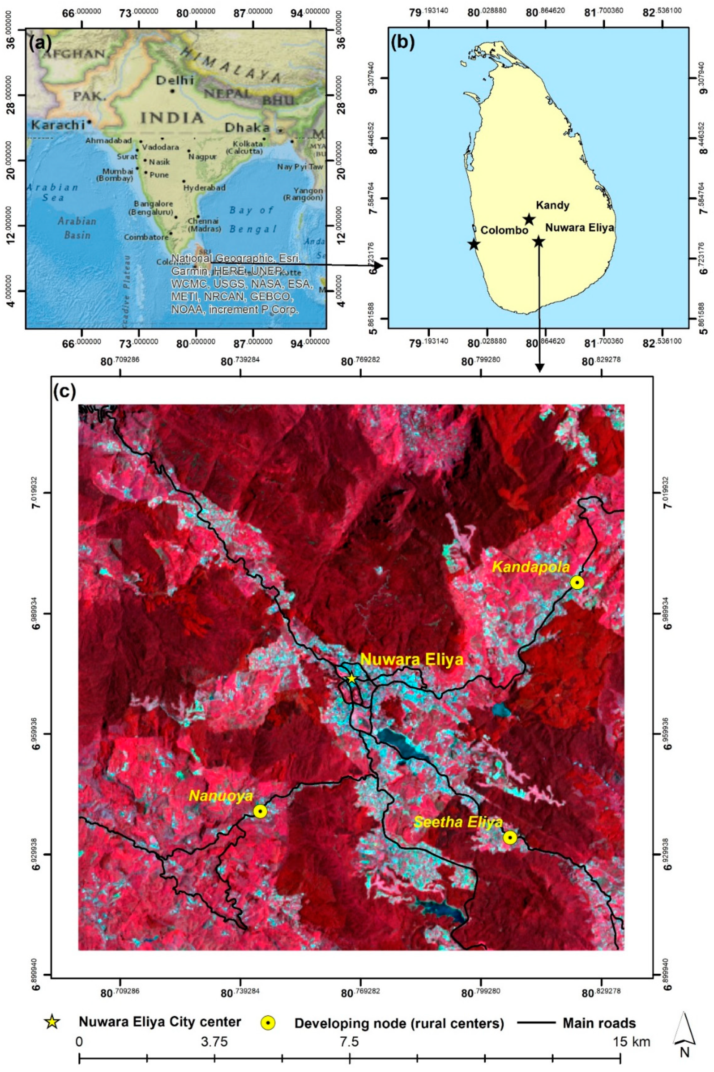
2.1. Study Area: Nuwara Eliya, Sri Lanka

The Nuwara Eliya area is located in the central highlands of Sri Lanka between 6°54′22.94″N and 7°2′28.53″N and 80°50′5.89″E and 80°41′57.23″E (Figure 1). The average elevation of the city is 1800 m above sea level. Nuwara Eliya receives an annual average rainfall of 1905 mm with peak rainfall from October to December. The daily mean temperature of Nuwara Eliya is 15.9 °C with an average low of 11.6 °C and an average high of 20.2 °C.

According to the Department of Census and Statistics of Sri Lanka, Nuwara Eliya has a multi-ethnic, multi-cultural population including Indian Tamil, Sinhalese, Sri Lankan Tamil, Sri Lankan Moor, Malay, and Burgher communities [33]. Over the last decade, the Nuwara Eliya area has undergone considerable development as a tourist city because it is one of the most attractive tourist destinations of Sri Lanka due to its cool natural environment. It is commonly known as the hill resort of Sri Lanka, or “Little England.” The Nuwara Eliya district has also been experiencing rapid urbanization with an estimated annual population growth rate of about 1.12% between 2012 and 2018 [34]. The population of Nuwara Eliya grew from 603,577 in 1981 to 711,644 in 2012 and is currently estimated to be over 800,000 [34]. The Nuwara Eliya district is about 1741 km² with an estimated population density of 438.3/km² [34]. The rapid urbanization has exerted pressure on land management and administration as well as sustainable urban planning.

2.2. Data Processing

Time-series Landsat 5TM and 8 OLI/TRS images obtained from the United States Geological Survey (USGS) website (http://earthexplorer.usgs) were used to extract LULC maps for 1996, 2006, and 2017. We selected atmospherically corrected pre-processed (<10% cloud-free) Landsat images (Level 2). Adhering to that criteria, we selected Landsat 5TM images for 24 March 1996 and 16 February 2006, and Landsat 8 OLI/TIRS for 18 March 2017. The selected images were georectified using the WGS84/UTM 44N projection system.

Table 1. Descriptions of the spatial data used in the study.

Data Type	Format	Scale/Resolution	Data Source	Year	Projection
DEM	Raster	30 m	United States Geological Survey (USGS)	2017	WGS84/UTM 44N
Slope	Raster	30 m	Extracted from DEM	2017	WGS84/UTM 44N
Road network	Vector	1:50,000	Survey Department, Sri Lanka	2017	WGS84/UTM 44N
Forest protection area	Vector	1:50,000	Forest Department, Sri Lanka	2010	WGS84/UTM 44N

shows the details of the other auxiliary data used for this study. The 30 m DEM was also downloaded from the USGS website to develop a slope map of the study area. The road network was extracted from a 1:50,000 topographic map obtained from the Survey Department of Sir Lanka. The forest reservation boundaries of the study area were extracted from forest cover maps obtained from the Forest Department of Sri Lanka. The auxiliary data was used to derive modeling variables used for the prediction of future LULC changes in the study area.

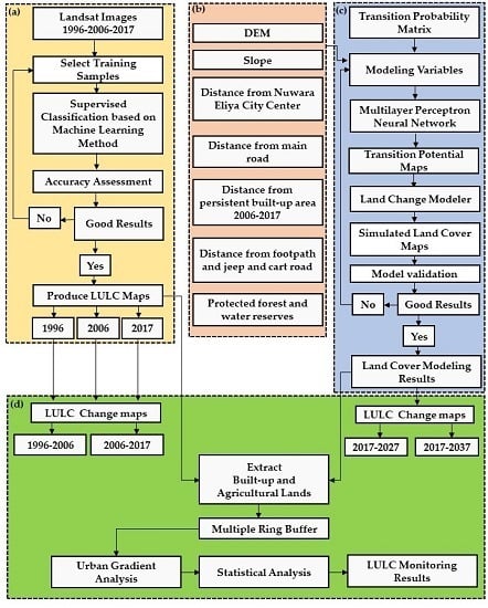
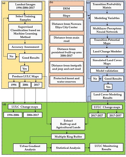
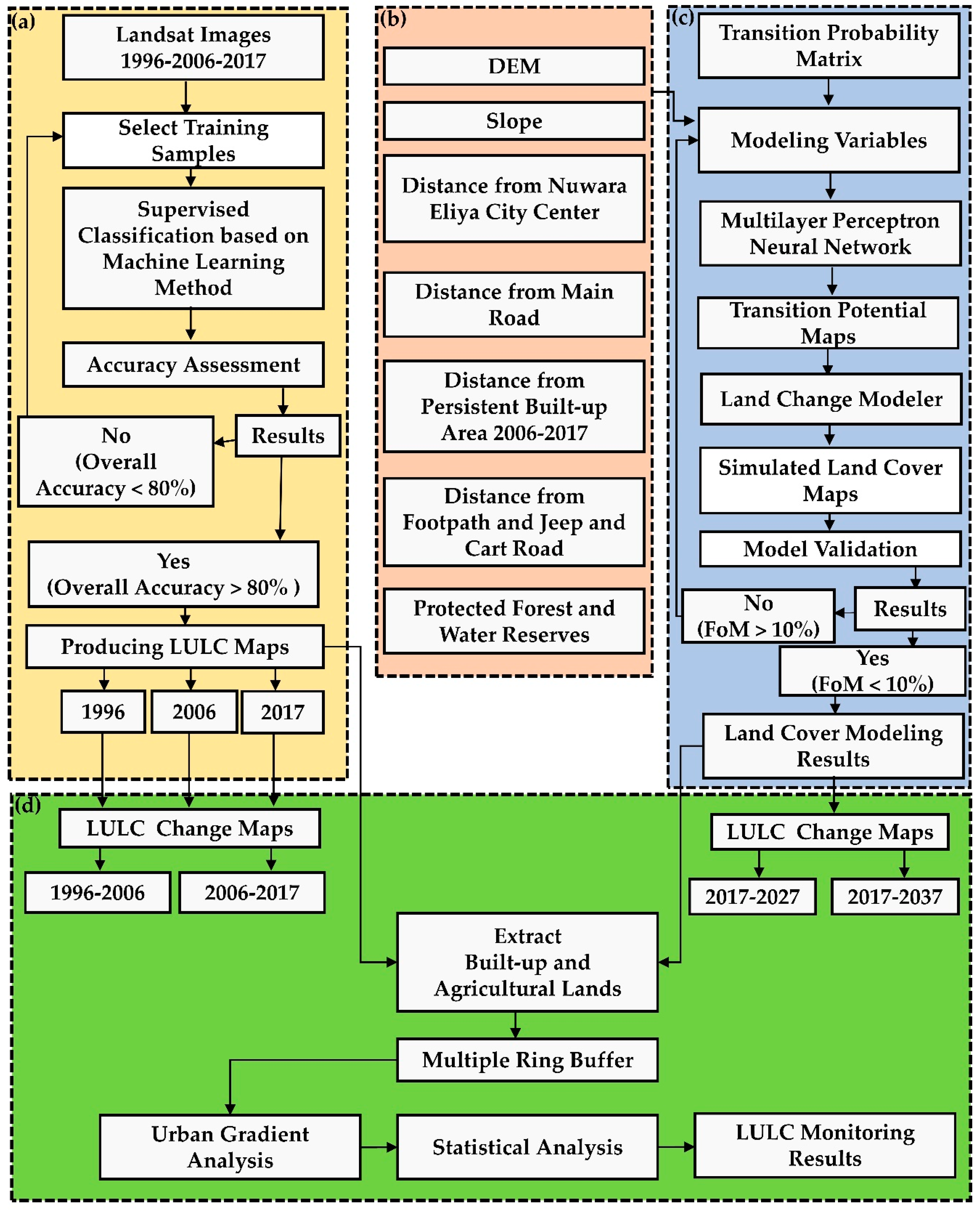
2.3. Overall Workflow

Figure 2 shows the overall workflow of the study to achieve aforesaid objectives with four primary steps viz., (a) LULC classification using machine learning algorithms based supervised classification and accuracy assessments; (b) selection of modeling variables; (c) prediction of the future LULC changes; and (d) assessment of LULC changes using urban–rural gradient analysis.

2.4. LULC Classification

In this study, we considered five LULC classes: built-up, forest, agriculture land, water, and other land (

Table 2. Description of the LULC classes used for classification.

Land Use/Cover	Description
Built-up	All impervious surfaces including urban, residential, industrial and institutional areas, transport utilities and all other impervious areas.
Forest	Areas including high and low-density evergreen forest over the year.
Agricultural land	Commercial and non-commercial agricultural areas (including tea and up-county vegetables).
Water	Areas covered by water bodies such as dams, lakes, rivers, reservoirs, and streams.
Other land	Bare land, grassland, and all LULC classes not accounted by the above four classes.

). LULC classification was then conducted as follows. First, we selected a pixel-oriented supervised classification method which is compatible with the primary data source categorized as medium resolution data (i.e., Landsat data). Second, we selected four types of classification methods facilitated by R software. R [36] is a free and open source statistical and computer graphic software generally used in various research fields for statistical computing and graphics [37]. One of the main opportunities of R is its wide range of machine learning image classifiers which allow pixel oriented image classification [37,38]. The methods used in this study included (i) support vector machines, (ii) K-nearest neighbor, (iii) random forest, and (iv) neural networks (See R Script provide in Annex B). In the process, the same set of training data were used to maintain the uniformity in the LULC classification for each year (i.e., 1996, 2006, and 2017). Hence, we generated four LULC maps for each year based on the adopted four types of classification methods.

In the third step, we sorted the LULC maps based on accuracy assessment and selected the maps with the highest value of both overall accuracy and kappa statistics. Following this selection criterion, we selected the LULC maps created by support vector machines for the years 1996, 2006, and 2017. Fourth, agreeing with previous researches [39,40,41,42], we adopted the majority filters and hybrid classification methods to resolve the problem of misclassification errors or salt and pepper noises that were generated by spectral confusion [39].

2.5. Accuracy Assessment

We conducted an accuracy assessment to determine the correctness of the LULC information derived from the Landsat data. We applied a stratified random sampling method [39,43] to cover all LULC types and generated 500 points for each year. Then, Google Earth historical imagery was used as reference data for accuracy assessment in 2006 and 2017. We could not obtain reference information for 1996 due to the low spatial resolution of Google Earth historical imagery. Hence, the topographic maps obtained from the Survey Department of Sri Lanka were used to assess the accuracy of the classified maps in 1996. Finally, we computed the user’s accuracy (accounting for errors of commission), producer’s accuracy (accounting for errors of omission), overall accuracy, and Kappa coefficient in each year using a confusion matrix [44,45]. This method is commonly used in similar studies, and details can be found elsewhere [46].

2.6. Land Change Modeler

The Land Change Modeler (LCM) is integrated into the TerrSet Geospatial Monitoring and Modeling software [47] to perform LULC change analyses, LULC prediction, and scenario simulation [48]. LCM provides a better understanding of LULC change patterns to support urban planning and sustainable development [49]. The LCM module is divided into three parts: (1) identification modeling variables based on past LULC changes and creation of potential transition maps between each LULC category by applying the Multilayer Perceptron Neural Network (MLP-NN); (2) preparation of transition area and transition probability matrices based on the Markov chain stochastic model using previous LULC maps to simulate future LULC; and (3) simulation and extrapolation of LULC maps, comparison of the simulated LULC maps with real maps to calculate LCM module accuracy, and production of predicted future LULC maps.

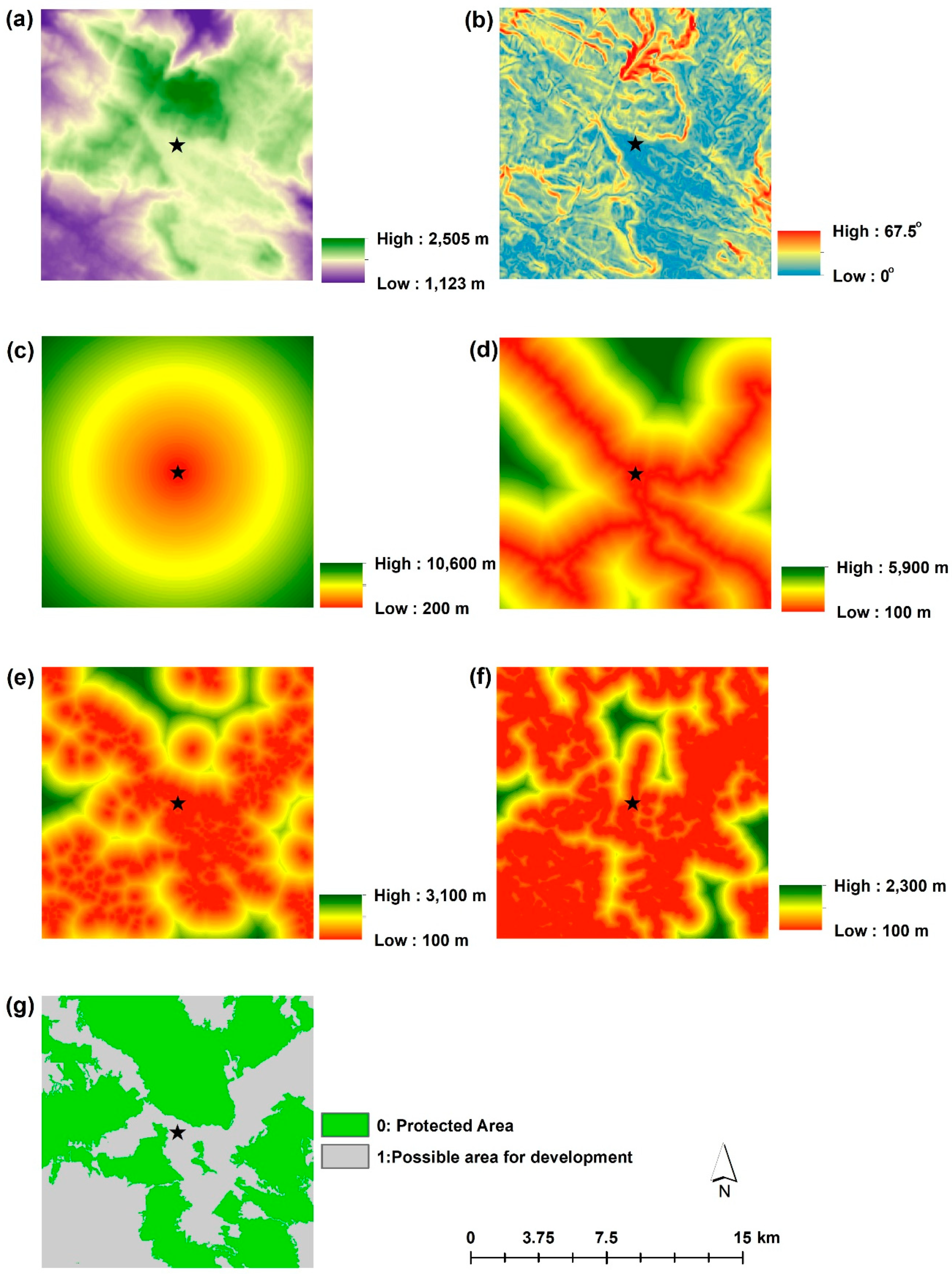
2.6.1. Modeling Variables Selection and Creating Transition Potential Maps

One of the critical steps in LULC modeling is to identify the best modeling variables that can explain the variation and allocation of LULC distribution when conducting spatiotemporal prediction [3,50,51]. In this study, we first defined seven modeling variables as driving forces of the LULC changes in the study area. These included: digital elevation model (DEM); slope; distance to central business districts (CBD); distance to the main road; distance from the persistent built-up area; distance from the footpath, jeep and cart road; and forest and water protection area (

Table 3. Description and importance of selected modeling variables.

Representative Factor	Description
DEM (meter)	Provide suitable areas for future development. For example, the lowland area is more inclined to be developed.
Slope (degree)	Provide suitable areas for future development. For example, some area which slopes down sharply should be developed into the grass, forest.
Distance from the main road (meter)	The road as the main transportation utility in the study area and it drives urbanization.
Distance from city center (meter)	According to the LULC maps from 1996 to 2017, the built-up area expanded from city center to the surrounding area. The city center manually demarcated as 6.973,902,78 N and 6.973,902,78 E.
Distance from footpath and jeep and cart roads (meter)	To provide for the future development of the road. The possible road development can be from converting jeep and cart roads into the main road and footpath into jeep and cart roads.
Distance from persistent built-up (meter)	The new built-up area always has been established around persistent built-up.
Protected area	Area limiting the development or difficult to change in a short time. During the past 21 years, the forest protection areas have not been changed due to the government policies on forest protection.

). All the modeling variables as spatial aspect were selected by considering the development pattern of the area while utilizing our knowledge about the study area. Other studies have shown that the best approach for variable selection based on study area characteristics, observed LUCCs overtime, and expert knowledge of the individual study areas [27,28]. After variable selection, we employed the fuzzy membership function to standardise all the modeling variables in order to reduce self-influence as variables had different ranges. Six variables, except for the protectd area, were standardized to a range of 0 to 1. The protected area was reclassified into a binary variable with values 0 and 1, i.e., 0 representing areas that cannot change and 1 representing areas that can change during the transition. To complete the first step in LCM, we then applied the MLP-NN module to create potential transition maps showing the potential of each transition at a given location in the entire study area (Figure 3). The MLP-NN was set at 10,000 iterations for each transition using dynamic automatic training and achieved accuracy values ranging from 83.23% to 92.42%. The accuracy values were all within the recommended accuracy rate of over 80% [47].

2.6.2. Transition Matrices

In the second step, we prepared the transition area and transition probability matrices based on the Markov chain approach using the 1996, 2006, and 2017 LULC maps produced in Section 2.4. The Markov chain model is a stochastic model designed to determine the probability of change from one state to the other. It is therefore advantageous in the quantification of conversion states and revealing the transfer rates among different LULC types [30]. However, the Markov model cannot determine the spatial extent of LULC changes [30]. By employing a Markov chain approach, the transition probability can be calculated based on past LULC maps [52]. Because of this characteristic, the Markov chain approach has been widely used to predict LULC composition by combining several models, including the MLP-NN model, cellular automata model, and a logistic regression model [53,54,55]. In this study, we used the Markov chain approach to calculate the transition probability area matrix using Equation (1) [56].

$$N_{t+1}= P_{matrix}\ast N_t$$

(1)

where $N_t$ is a state vector of LULC at time $t$, $N_{t+1}$ is a state vector of LULC for the same types at time $t+1$, $P_{matrix}$ is a matrix that expresses the LULC transition probability from time $t$ to $t+1$.

The transition area matrix was obtained based on two LULC maps (1996 and 2017) expressed as Equation (2):

$$\mathrm{A}=\left[\begin{array}{ccc}{A}_{11}& \cdots & A_{1n}\\ ⋮& \ddots & ⋮\\ A_{n1}& \cdots & A_{nn}\end{array}\right]$$

(2)

The transition matrices from 1996–2006, 2006–2017, and 1996–2017 periods were examined by employing the Markovian transition estimator module in TerrSet version 18.31. The transition matrix between 1996 and 2006 was used to simulate the 2017 LULC map for model validation with the actual 2017 LULC map. The transition matrix between 2006 and 2017 was used to predict LULC maps for the years 2027 and 2037.

2.6.3. LULC Simulation and Model Validation

In the third (final) step, we used the 1996 and 2006 LULC maps to predict and produce the simulated 2017 LULC map. Model validation was then carried out by comparing the simulated 2017 LULC map to the observed 2017 LULC map produced in Section 2.4 above. Model validation was used to understand the effectiveness of the LCM [9,27,57]. We used Cohen’s Kappa coefficient [58] to check the agreement between the simulated and observed 2017 LULC maps. Equation (3) was used to derive the Cohen’s Kappa coefficient:

$$\mathrm{K}=\frac{P_0-P_e}{1-P_e}=1-\frac{1-P_0}{1-P_e}$$

(3)

where K represents the probability of agreement between two layers; $P_0$ is the relative observed agreement among layers; and $P_e$ is the hypothetical probability of chance agreement. Kappa values less than zero indicate no agreement between two maps; 0 to 0.2 indicate the relationship is slight; 0.21 to 0.4 indicate the relationship is fair; 0.41 to 0.6 indicate the relationship is moderate; 0.61 to 0.8 indicate the result is substantial while kappa values ranging from 0.81 to 1 indicate almost perfect agreement [59,60].

Since the application of Kappa evidence may not be sufficient to evaluate simulation efficiency correctly [61], we employed figures of merit (FoM) to cross-check the results [9,32]. To validate our evaluation, the observed and simulated 2017 LULC maps were cross-tabulated. The FoM was derived using Equation (4):

$$FoM=\frac{H}{H+M+F}\ast 100\%$$

(4)

where H, M, and F are the hits, misses and false alarms, respectively. After validating the model, we simulated future LULC changes and produced two LULC maps for the years 2027 and 2037.

2.7. Urban–Rural Gradient Analysis

“Gradient” can be defined as the variation in the values of a given variable [5]. Gradient analysis can be considered as an appropriate method to analyze landscape patterns [62]. This method was developed in the context of vegetation analysis [63]. During the past decades, gradient analysis has been widely used to capture the spatial and temporal variation of environmental variables with distance [3,5,64]. Several studies have demonstrated the applicability of gradient analysis in assessing land use dynamics from the city center to rural areas [32,65]. Nuwara Eliya developed based on the single core concepts. Development pattern shows the urban area to rural surrounding areas. Thus, we hypothesized that urban–rural gradient analysis is useful to understand the changing pattern of built-up and agriculture land. In addition, gradient analysis has also been used to analyze the decrease of agricultural land and the increase of built-up land [3]. In this study, we created 200 m multiple ring buffer zones (concentric circles) from the city center of Nuwara Eliya to extract LULC information. A total of 38 buffer zones were created. We assessed agricultural and built-up land changes in each buffer zones for the periods, 1996–2006, 2006–2017, 2017–2027, and 2017–2037. We then performed a linear regression analysis to find the relationship between changes in agricultural land and built-up land [3].

3. Results

3.1. Accuracy of LULC Maps

A comprehensive summary of the accuracy assessment results in each year is presented in

Table 4. Accuracy assessments of the LULC types.

Accuracy	LULC Category	1996	2006	2017
User’s accuracy (%)	Built-up	80.9	93.3	94.0
	Forest	90.2	94.3	92.5
	Agricultural land	84.3	93.4	94.4
	Other land	81.0	71.4	80.5
	Water	80.0	89.7	92.3
Producer’s accuracy (%)	Built-up	80.9	93.3	94.0
	Forest	85.1	95.8	94.7
	Agricultural land	87.0	91.2	91.2
	Other land	81.0	71.4	89.2
	Water	72.7	92.9	92.3
Overall accuracy (%)		85.0	93.0	92.0
Kappa Coefficient		0.80	0.90	0.90

. The accuracy assessment results show that the kappa coefficients achieved were 0.8, 0.9, and 0.9 and overall accuracies were 85%, 93%, and 92% for the 1996, 2006, and 2017 LULC maps, respectively (See

Table A1. Error matrix for the classified 1996 land use/cover map.

Classified Data	Reference Data
	Built-up	Forest	Agricultural Land	Other Land	Water	Total	User’s Accuracy (%)
Built-up	72	8	6	3	0	89	80.9
Forest	2	165	10	3	3	183	90.2
Agricultural land	5	17	140	2	2	166	84.3
Other land	2	2	3	34	1	42	81.0
Water	0	2	2	0	16	20	80.0
Total	81	194	161	42	22	500
Producer’s accuracy (%)	88.9	85.1	87.0	81.0	72.7

Overall Accuracy (%) = 85%.

,

Table A2. Error matrix for the classified 2006 land use/cover map.

Classified Data	Reference Data
	Built-up	Forest	Agricultural Land	Other Land	Water	Total	User’s Accuracy (%)
Built-up	98	2	5	0	0	105	93.3
Forest	3	182	8	0	0	193	94.3
Agricultural land	4	5	155	1	1	166	93.4
Other land	0	0	1	5	1	7	71.4
Water	0	1	1	1	26	29	89.7
Total	105	190	170	7	28	500
Producer’s accuracy (%)	93.3	95.8	91.2	71.4	92.9

Overall Accuracy (%) = 93%.

and

Table A3. Error matrix for the classified 1996 land use/cover map.

Classified Data	Reference Data
	Built-up	Forest	Agricultural Land	Other Land	Water	Total	User’s Accuracy (%)
Built-up	110	3	3	1	0	117	94.0
Forest	5	160	7	1	0	173	92.5
Agricultural land	3	2	135	2	1	143	94.4
Other land	2	3	2	33	1	41	80.5
Water	0	1	1	0	24	26	92.3
Total	120	169	148	37	26	500
Producer’s accuracy (%)	91.7	94.7	91.2	89.2	92.3

Overall Accuracy (%) = 92%.

in Appendix A). The classification errors observed emanated from spectral confusion between LULC classes with similar spectral responses, e.g., spectral confusion between forests versus some active agricultural lands or grasslands and vice versa; and built-up lands versus some bare lands and vice versa. Nonetheless, the Kappa coefficients and overall accuracy values achieved were sufficiently high (>80%) as recommended by the authors of [66] and therefore considered to be acceptable.

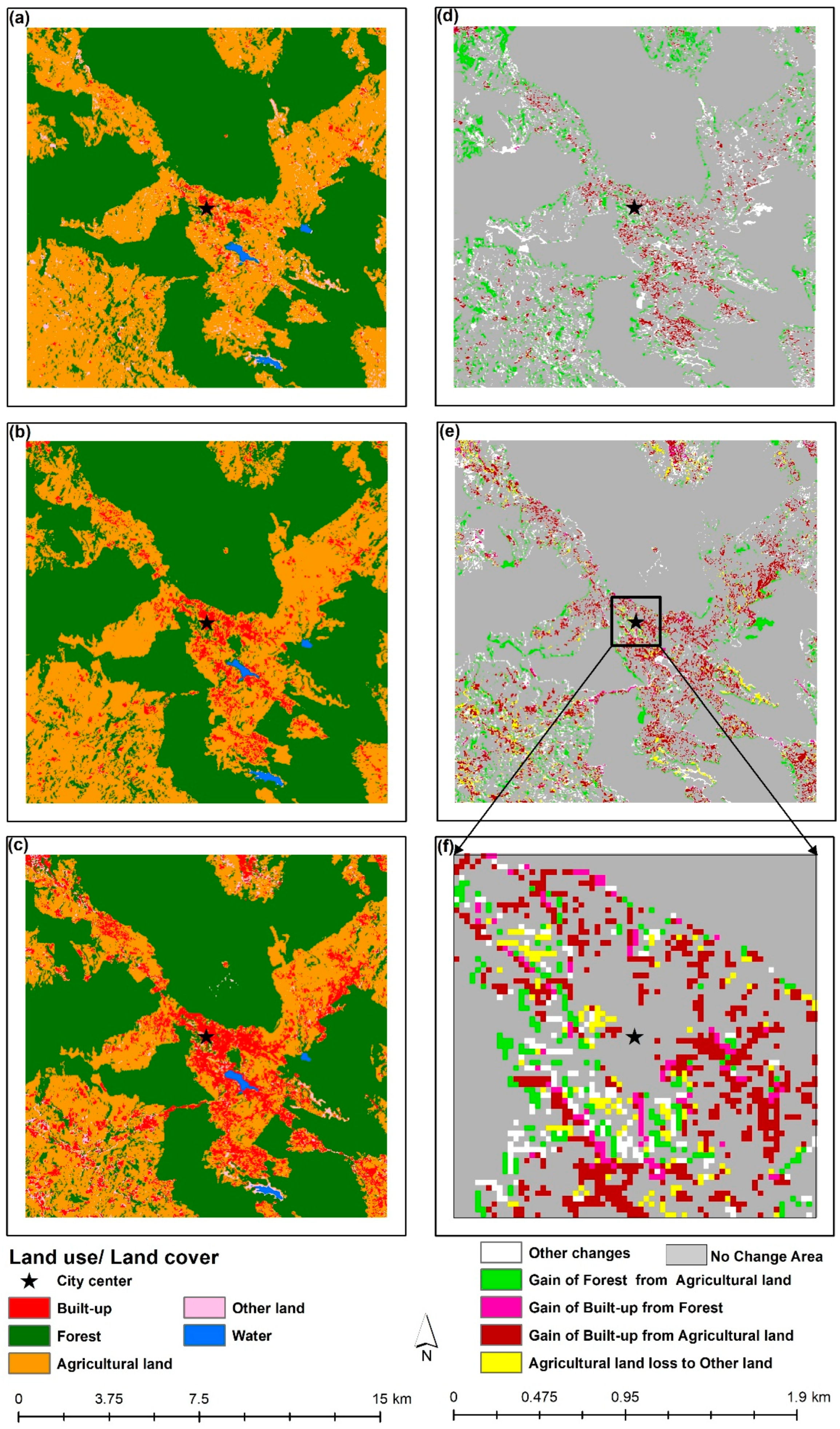
3.2. Spatial-temporal Changes in LULC

Figure 4a–c shows the classified LULC maps of the study area for the years 1996, 2006, and 2017, respectively. The results show that in 1996, the city center primarily consisted of built-up land while all other areas outside the city center consisted of other land uses, mainly agricultural lands and forests. In 2006, the built-up lands spread towards the southern, eastern, southwestern, and northwestern regions of the city. The results show that forest land increased from by 157.6 ha (i.e., 13,076.7 to 13,234.3) between 1996 and 2017 with a relatively slight annual gain rate of 7.5 ha/year.

Figure 4d,e show the LULC change maps for the periods of 1996–2006 and 2006–2017. According to the results, there has been a substantial conversion of agriculture land to built-up land over the past 21 years (1996–2017). Agricultural land showed a slight reduction trend from 1996 to 2006 (8503 ha to 8086 ha) and a notable reduction trend (8086 ha to 6584 ha) from 2006 to 2017 (

Table 5. Details of the land use and land cover changes in Nuwara Eliya in 1996, 2006, and 2017.

Land Use/Cover	1996		2006		2017
	Area (ha)	%	Area (ha)	%	Area (ha)	%
Built-up	289.9	1.3	785.5	3.5	2080.4	9.3
Forest	13,076.7	58.2	13,502.1	60.1	13,234.3	58.9
Agricultural land	8503.2	37.9	8085.5	36.0	6583.9	29.3
Other land	511.8	2.3	6.0	0.0	481.8	2.1
Water	73.4	0.3	75.9	0.3	74.6	0.3
Total	22,455.0	100.0	22,455.0	100.0	22,455.0	100.0

). During the 1996–2006 period, agricultural lands decreased by 417.7 ha corresponding to an annual loss rate of 41.8 ha/year (

Table 6. Land use and land cover change matrix (ha), 1996–2006.

2006
1996	Built-up	Forest	Agricultural Land	Other Land	Water	Grand Total
Built-up	277.7	2.1	9.9	0.3	0.0	289.9
Forest	12.1	12,347.9	707.6	0.5	8.6	13,076.7
Agricultural land	434.5	1088.5	6972.6	4.0	3.7	8503.2
Other Land	59.7	55.1	390.9	0.8	5.4	511.8
Water	1.6	8.6	4.6	0.5	58.1	73.4
Grand total	785.5	13,502.1	8085.5	6.0	75.9
Net change	495.6	425.3	−417.7	−505.8	2.5
Annual change	49.6	42.5	−41.8	−50.6	0.3
Annual change rate (%)	10.5	0.3	−0.5	−35.9	0.3

). A much higher decrease of 1507.7 ha in agricultural lands translating to an annual loss rate of 136.5 ha/year was observed during the 2006–2017 period (

Table 7. Land use and land cover change matrix (ha), 2006–2017.

2017
2006	Built-up	Forest	Agricultural Land	Other Land	Water	Grand Total
Built-up	762.2	5.3	6.7	9.8	1.5	785.5
Forest	146.7	12,529.4	727.8	90.3	7.8	13,502.1
Agricultural land	1166.9	694.9	5848.6	368.7	6.5	8085.5
Other land	0.4	0.2	0.3	4.7	0.5	6.0
Water	4.3	4.5	0.5	8.3	58.2	75.9
Grand total	2080.4	13,234.3	6583.9	481.8	74.6
Net change	1294.9	−267.8	−1501.7	475.7	−1.3
Annual change	117.7	−24.3	−136.5	43.2	−0.1
Annual change rate (%)	9.3	−0.2	−1.9	48.9	−0.2

). Overall, agricultural land continuously decreased from 1996 to 2017, translating into a total loss of 1919 ha and an annual loss rate of 91.4 ha/year or −1.2% annual change rate (ACR) (

Table 8. Land use and land cover change matrix (h), 1996–2017.

2017
1996	Built-up	Forest	Agricultural Land	Other Land	Water	Grand Total
Built-up	284.9	0.2	3.2	1.7	0.0	289.9
Forest	103.8	12,478.7	440.9	48.9	4.5	13,076.7
Agricultural land	1531.1	711.8	5872.8	386.1	1.4	8503.2
Other land	159.7	40.5	266.7	45.0	0.0	511.8
Water	1.1	3.2	0.4	0.1	68.7	73.4
Grand total	2080.4	13,234.3	6583.9	481.8	74.6
Net change	1790.6	157.6	−1919.3	−30.1	1.3
Annual change	85.3	7.5	−91.4	−1.4	0.1
Annual change rate (%)	9.8	0.1	−1.2	−0.3	0.1

Note: Annual change rate (ACR) is calculated as $A=\left(\sqrt[j-i]{\frac{A_j}{A_i}}-1\right)\ast 100$. A_i and A_j are the areas of each land cover category at time points i (time 1) and j (time 2), respectively.

).

The loss of agricultural land to built-up land was confirmed by the increase in the built-up area from 289.9 ha in 1996 to 785.5 ha and 2080.4 ha in 2006 and 2017, respectively. This change represented a total gain of 1790.6 ha and an ACR of 9.8% in built-up land between 1996 and 2017 (Table 8). On the other hand, the loss from other lands (grasslands and bare lands) was relatively insignificant during the temporal study extent.

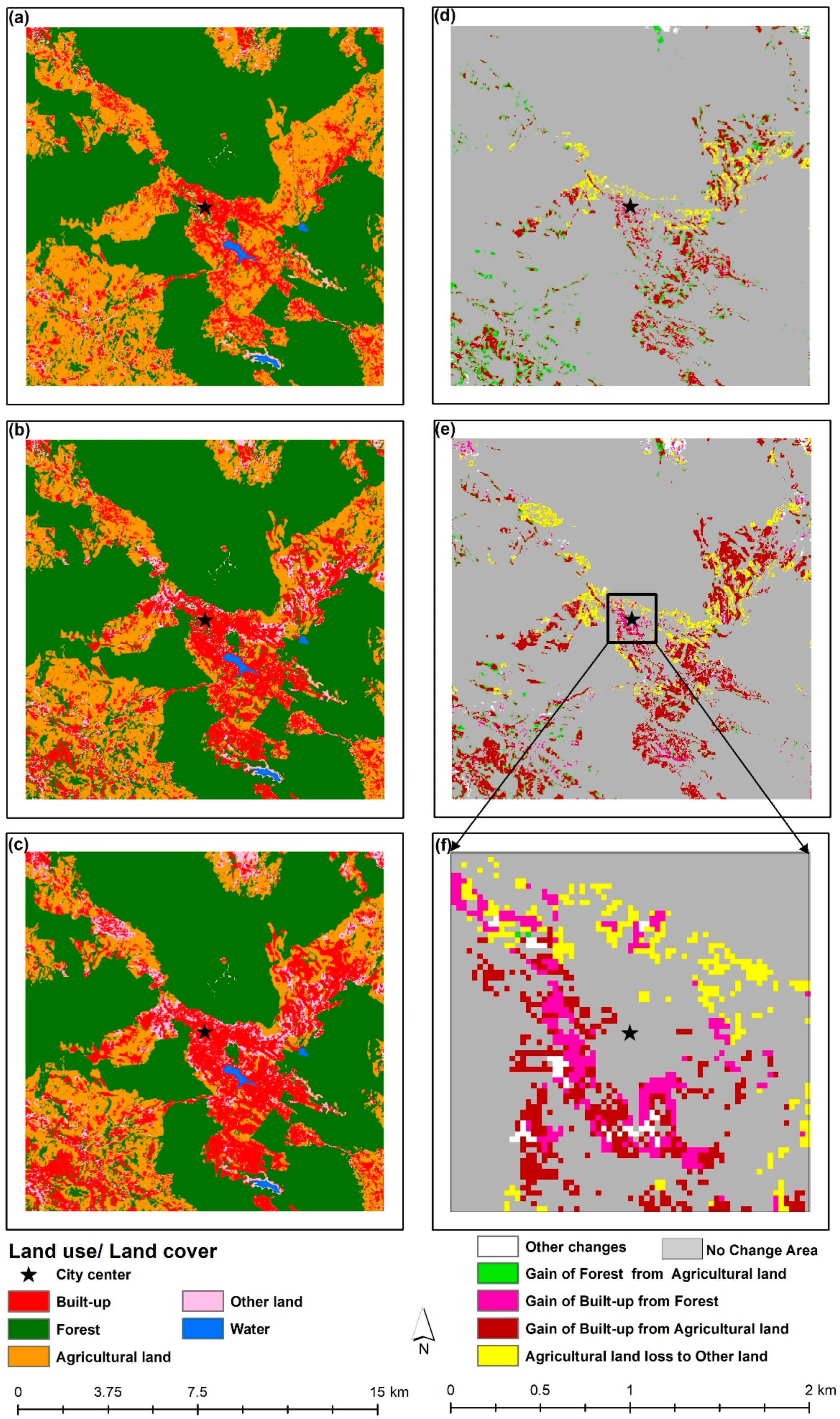
3.3. LULC Modeling and Simulation

Before simulating future LULC, we validated our model by comparing the observed and simulated 2017 LULC maps using Cohen’s Kappa coefficient and the FoM. The model validation results were 77.23% and 9.79% which were acceptable [32,61]. Thereafter, the model was used to simulate future LULC maps for 2027 and 2037 as shown in Figure 5b,c, respectively. According to the results, most of the central part of the study area will be covered by built-up lands in 2027 and 2037. Further, the built-up area will spread toward the eastern, southern, and southwestern regions of the city. The simulation results show between 2017 and 2027; the built-up area will increase by 13.4% and further increase by 17.7% between 2017 and 2037 (

Table 9. Details of the land use and land cover changes in Nuwara Eliya Area in 2027 and 2037.

Land Use/Cover	2027 Area (ha)	%	2037 Area (ha)	%
Built-up	3012.7	13.4	3973.1	17.7
Forest	13,785.8	61.4	13,298.9	59.2
Agricultural land	4768.8	21.2	3954.7	17.6
Other land	813.1	3.6	1153.7	5.1
Water	74.6	0.3	74.6	0.3
Total	22,455.0	100.0	22,455.0	100.0

). The predicted annual increase in built-up land will be around 93.2 ha/year and 94.6 ha/year translating into ACRs of 3.8% and 3.3% for the 2017–2027 and 2017–2037 periods, respectively (

Table 10. Land use and land cover change matrix (ha), 2017–2027.

	2027
2017	Built-up	Forest	Agricultural Land	Other Land	Water	Grand Total
Built-up	2054.4	0.0	0.0	26.0	0.0	2080.4
Forest	8.6	13,220.6	0.0	5.2	0.0	13,234.3
Agricultural land	949.7	565.3	4768.8	300.1	0.0	6583.9
Other land	0.0	0.0	0.0	481.8	0.0	481.8
Water	0.0	0.0	0.0	0.0	74.6	74.6
Grand total	3012.7	13,785.8	4768.8	813.1	74.6	22,455.0
Net change	932.2	551.5	−1815.0	331.3	0.0
Annual change	93.2	55.2	−181.5	33.1	0.0
Annual change rate (%)	3.8	0.4	−3.2	5.4	0.0

and

Table 11. Land use and land cover change matrix (ha), 2017–2037.

	2037
2017	Built-up	Forest	Agricultural Land	Other Land	Water	Grand Total
Built-up	2030.6	0.0	0.0	49.9	0.0	2080.4
Forest	170.3	12,986.9	0.0	77.1	0.0	13,234.3
Agricultural land	1772.3	311.9	3954.7	545.0	0.0	6583.9
Other land	0.0	0.0	0.0	481.8	0.0	481.8
Water	0.0	0.0	0.0	0.0	74.6	74.6
Grand total	3973.1	13,298.9	3954.7	1153.7	74.6	22,455.0
Net change	1892.7	64.5	−2629.2	671.9	0.0
Annual change	94.6	3.2	−131.5	33.6	0.0
Annual change rate (%)	3.3	0	−2.5	4.5	0

).

On the other hand, agricultural land will continue declining. From 2017, the loss of agricultural land is predicted around 21.2% and 17.6% by 2027 and 2037, respectively. The predicted annual decrease in agricultural land will be around 181.5 ha/year and 131.5 ha/year translating into ACRs of −3.2% and −2.5% for the 2017–2027 and 2017–2037 periods, respectively. The results show that the forest may increase in size at a very relatively low rate of about 0.4% between 2017 and 2027 (Table 10).

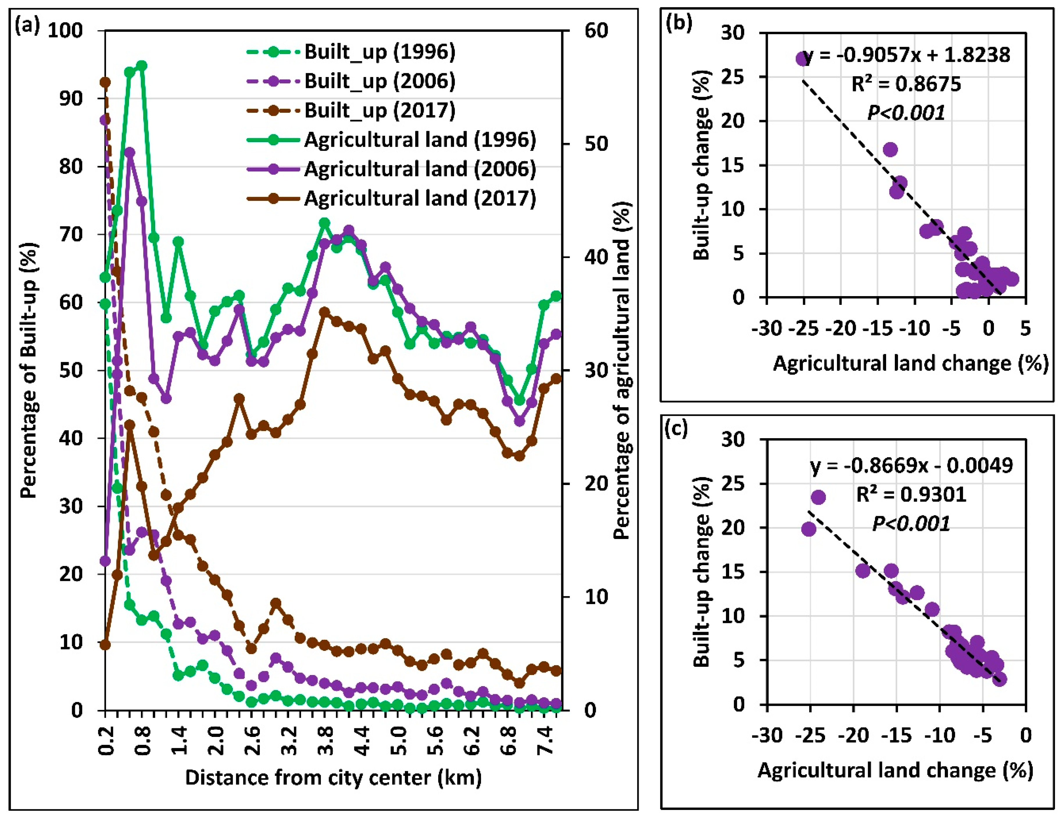
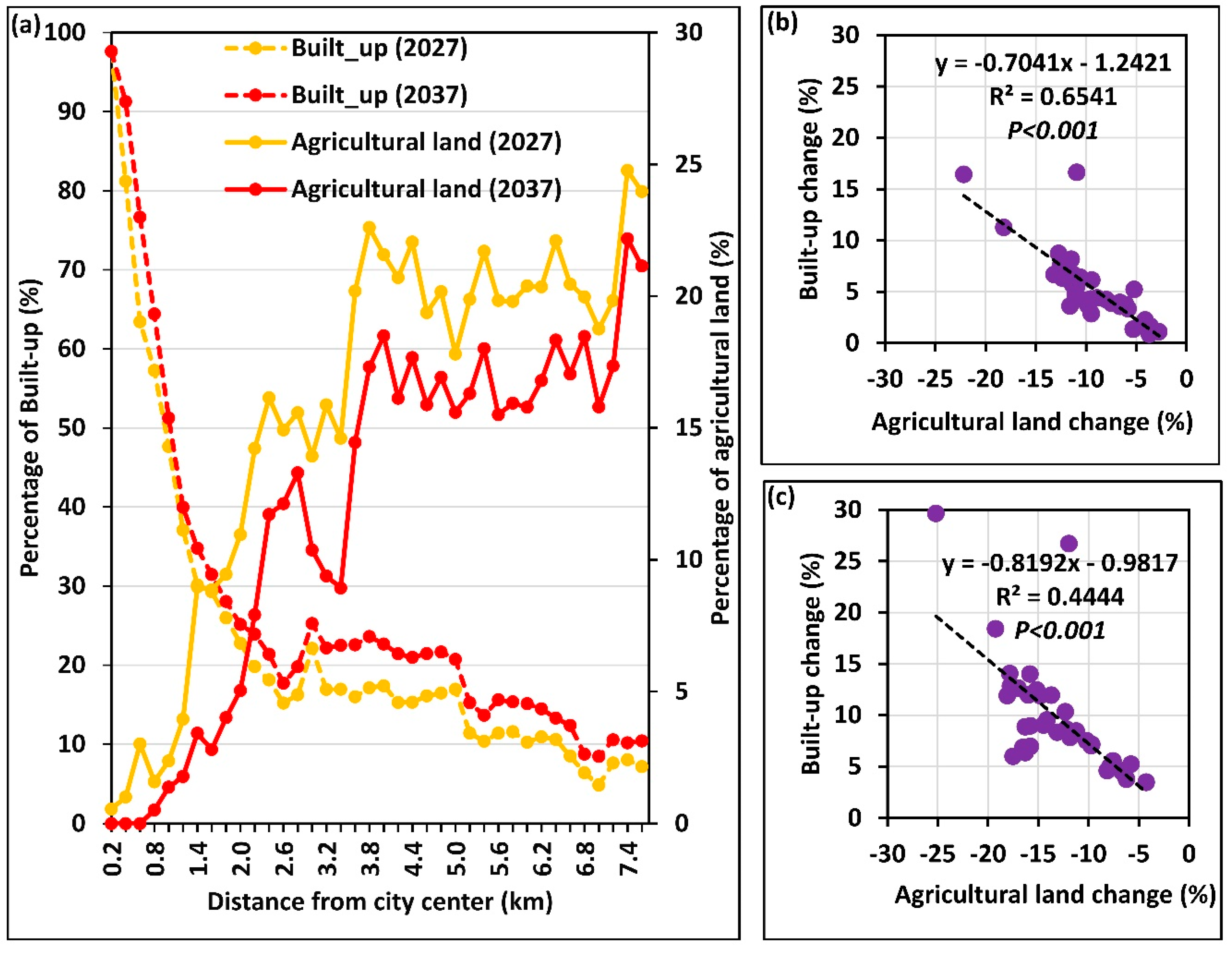
3.4. LULC Changes along the Urban–rural Gradient

Figure 6a shows the distribution of the built-up lands and agricultural land across the urban–rural gradient zones from 1996 to 2017. The percentage of built-up land near the city center exhibits a rapid increase from 59.8% in 1996 to 86.8%, and 92.4% in 2006 and 2017, respectively. Similarly, the percentage of agricultural land shows a continuous decrease of 38.2%, 13.2%, and 5.8% in 1996, 2006, and 2017, respectively.

Figure 7a shows the spatial pattern of predicted built-up and agricultural land percentages in 2027 and 2037 compared to the base year (2017). The urban–rural gradient analysis shows a rapid decrease in the percentage of agricultural land from 1996 to 2037. The mean decrease in agricultural lands is estimated at 36.9%, 33.7%, 25%, 15.6%, and 11.9% while mean increase in built-up lands is estimated at 5.2% in 1996, 9.9% in 2006, 17.4% in 2017, 22.8% in 2027, and 27.2% in 2037, respectively. The gradient zones with >10% of built-up land were at a distance of 1.2 km in 1996, 2 km in 2006, and 3.4 km distance in 2017. The predicted results show that the gradient zones with >10% of built-up lands will shift to a distance of 6.4 km in 2027 and 6.6 km in 2037. The results indicate that these regions also have the highest loss of agricultural land from 1996 to 2037.

Statistical analysis shows that agricultural land changes had a significant negative relationship with built-up land changes between 1996–2006 and 2006–2017. However, the correlation will decrease during the 2017–2027 and 2017–2037 periods (Figure 6b,c, and Figure 7b,c). The predicted results indicate that a similar pattern can be expected in 2027 and 2037. The forest cover will not undergo significant changes, and more agricultural land will be replaced by built-up areas.

4. Discussion

4.1. Spatiotemporal LULC Changes and Driving Forces

In this study, we assessed the LULC changes of the Nuwara Eliya area over the last 21 years (1996–2017) and predicted possible LULC changes for the next two decades (2017–2037). Our results indicate that rapid urbanization has occurred in the Nuwara Eliya area during the last two decades, which has dramatically changed the urban landscape. The region experienced rapid development in the tourism sector over the previous decades with significant growth during the last decade (2006–2017) as the Sri Lankan Civil War ended in 2009. Therefore, new facilities were established to cater to growing social and economic demands from the growing population. Compared to the year 2009, the accommodation capacity of the hill country of Sri Lanka increased by 53% in 2016, while the occupancy rate increased from 42.2% to 75.24% during the same period. These figures confirm that there was an increase in infrastructure development as well as a boost in tourism during the last decade. Further, the development of transportation systems after 2009 was also intensified due to the rapid urbanization of the city [32]. Most of the development projects were associated with the development of accessibility across the country, especially the hill regions of Sri Lanka including the Nuwara Eliya area. Thus, this may have affected the rapid changes in the tourism sector of the study area. Policymakers and planners are notably concerned about this pattern of urbanization as it is vital in effective decision-making [67]. However, these studies are rare in the Sri Lankan context. As a developing city aiming to boost its tourism industry, the Nuwara Eliya area must be developed according to an effective plan that maintains its scenic beauty while developing the required infrastructure. According to the Tourism Vision 2025 of the Ministry of Tourism Development [68], the Nuwara Eliya area will develop into a national tourism hub. Therefore, predicted LULC changes might guide the proper planning of effective, efficient, and sustainable use of resources.

LULC maps for the years 1996, 2006, and 2017 show an increasing trend of built-up land in the Nuwara Eliya area (Figure 4). From 1996 to 2006, built-up areas increased by 495.6 ha with an ACR of 10.5%. It also increased up to 1294.9 ha (ACR = 9.3%) during the 2006–2017. Previous studies have shown that forest areas become more vulnerable to development because of urbanization pressure in other Asian mountain cities such as Kandy in Sri Lanka [11], Bengaluru in India [49], Kathmandu in Nepal [10], Baguio in the Philippines [5], Bogor in Indonesia [5], Dalat in Vietnam [5], and Islamabad in Pakistan [69]. However, the Nuwara Eliya area exhibits unique characteristics in the urbanization trend; instead of dramatic decreases in forest areas, agricultural land has significantly decreased. The results revealed that nearly 60% of the study area is under forest cover which could be attributed to the existence of forest reserves in the area. For the last 21 years, the study area has been dominated by forest because of government policies on conserving forest resources in upper catchment areas and initiatives taken by the upper watershed management project of the Asian Development Bank [70,71]. Hence, it means that the pressure of urbanization has exerted on agricultural lands and other lands (Table 8). The decreasing trend of agricultural land was significant during the second time point (from 2006 to 2017) compared to the first time point (between 1996–2006) (Table 6 and Table 7). The built-up area shows a similar (but inverse) pattern from 1996 to 2017; hence, the reduction of green areas was significant. Responding to the policy changes, the forest area increased during the first time point (1996–2007). However, there was some reduction (24.3 ha/year) during the second time point (2006–2017) as some unreserved forest areas were cleared for other land uses (Table 7). According to our LULC forecasts, the forest cover may remain without significant changes (Table 9), akin the government policies. If the current forest resource reservation and restoration policies for upper catchment areas remain, forest areas may increase by 552.5 ha with 55.2 ha/year during the 2017–2027 period. However, because of the saturation of forest reserves and rapid urbanization pressure, some forest areas may be deforested between 2027 and 2037. Thus, when we consider the 2017–2037 period, the annual gain of forest cover will remain small at 3.2 ha/year. The predicted maps show that similar pattern of increasing built-up areas and declining agricultural areas can be expected for 2027 and 2037. These changes are most notable in northeastern, southern, and southwestern regions of the area. Our results indicate an increasing trend of land use conversion (from agricultural land to built-up land) at 5.1%, 14.4%, 14.4%, and 26.9% in 1996–2006, 2006–2017, 2017–2027, and 2017–2037 periods, respectively. A similar pattern of agricultural land loss can be seen in previous studies conducted in P.O. Lwin in Myanmar [5], Hangzhou in China [3], Tianjin in China [72], Baguio in the Philippines [5], Tehran in Iran [44], and Kandy in Sri Lanka [11].

In model validation, Kappa and FoM reached 77.23% and 9.79%, respectively. We can confirm the strong relationship between observed and simulated results, if, the Kappa value reported more than 60%. Moreover, the FoM value is used to test the changes between two-time points i.e., changes that occurred from 2006-2017 as well as 1996 to 2017 in this study. The FoM value is influenced by LULC categories, annual change rate, and transition steps. For example, Subasinghe et al., simulated changes in the Colombo metropolitan area with three LULC categories and reached FoM of 15.06% in 2016 [32]. Sloan and Pelletier simulated forest-cover changes and reached FoM of 8.36% in 2012 [73], which was also considered as accepted. The most important reason why we cannot reach a high FoM value is that the other LULC category has a significant change from 1996 to 2017. As policy changes reserve the forests, during the first time point (1997–2006) a significant portion of marginally suitable lands (mainly bare lands and grasslands) converted to agricultural lands. However, during the second time point (2006–2017), some of those were reconverted to bare or grasslands due to poor productivity and economic return from those lands. Therefore, the FoM of 9.76% in this study can be accepted for further research.

In this study, we selected seven modeling variables as possible driving forces of future change. When selecting modeling variables, our selection was limited to the variables with the spatial property because these variables do not show frequent changes over time. The simulation was predicted possible future changes in the next 20 years based onstage of 2017, assuming no natural disasters, no changes in human factors or policies. According to the simulation results, if the current condition (2017 condition) will continue, about 1772.3 ha of cropland will change into built-up (Figure 5, Table 10 and Table 11) by 2037, which can make a significant change to socio-economic conditions of the area.

When predicting future LULC changes, 2017 was considered as the base year to quantify the changes along with the urban–rural gradient analysis. According to the predictions, LULC shows minimum changes over time in near the city center as the area is already saturated by built-up land. Beyond the city center, agricultural land shows further loosing while built-up areas are increasing over time. The average agricultural land percentage decreases by 9.4% during 2017–2027 and 13% during 2017–2037. Built-up land demonstrates a significant upward trend in the predicted result with increasing rates of 5.4% (2017–2027) and 9.7% (2017–2037). The change patterns in built-up and agricultural land show a strong significant negative relationship in both periods (Figure 6b,c). Although not much consistent as the 1996–2017 period, future predictions also show the same trend (Figure 7b,c). This result confirms that urbanization pressure has already reached the peripheral areas from the city center and will continuously move to the peripheral areas. This relationship can be attributed to the shifts in the urbanization patterns in the Nuwara Eliya area.

The urbanization pattern of the study area is different from other cities in Sri Lanka, such as Colombo and Kandy. The forest protection policies and topological and geomorphological constant have been directly contributed to more urban development pressure. These barriers have also contributed to the decreasing availability of the land for urban development. The urban development shows a scattered urbanization pattern during the temporal study extent. It has directly been influenced by the road network. More built-up patches were observed along with the road network. The new built-up patches were developed near the rural centers (Figure 4). Thus, the urbanization pattern of the study area shows a different scatted pattern compared with other major cities in Sri Lanka such as Colombo and Kandy. Colombo is a coastal city [32] while Kandy as a hilly city [11].

Moreover, we noted that the present urbanization process of the study area is not properly planned, and it has negatively affected the scenic beauty of the city. Thus, if this unplanned urbanization continues, it will lead to several environmental issues such as air pollution [74], water pollution [5], traffic congestion [67], and increasing land surface temperature [75,76,77]. Thus, policymakers must consider the rapid urbanization pattern of the city and introduce proper landscape and urban planning in the future to maintain the city’s natural beauty and ensure that the nation’s tourism industry is sustainable. The green-based development would help to enhance the natural beauty and minimize the destructive impacts associated with urbanization [78,79].

4.2. Landscape and Urban Planning in Nuwara Eliya

As most of the forest areas of the study area are forest reserves, urbanization pressure has been directed towards agricultural land. This situation may be unavoidable under the present policy implementations on land use and development of the tourism sector. However, upcountry agriculture plays a vital role in supplying exotic vegetables, fruits, cut flowers, and world-famous upland Ceylon tea to the local and international markets as most of those are unique to the upcountry landscape. The tourism sector is flourishing with these agricultural products, and their reduction may negatively affect the area’s tourism industry and socioeconomic conditions.

The urban–rural gradient analysis demonstrates that the city center is already saturated with built-up land that is extending to peripheral areas along the main access roads from the city center. Hence, agriculture in the area may be in peril. To control the clearing of agricultural land for built-up areas, policies that maximize land utilization such as those promoting storied buildings instead of single-story buildings without harming the existing British colonial style city architecture should be implemented [13]. Local governments must formulate and implement new policies and facilities for other development concerns such as proper waste management and storm-water drainage to maintain the region’s scenic beauty. Adequate implementation for existing rainwater harvesting policy also may help minimize the effects of increasing surface runoff due to land use changes. A demand assessment of fresh fruits, vegetables, and cut flowers may also help clarify the requirements of the growing tourism industry which could then further support the sustainability of the sector.

Land degradation has been identified as one of the most critical problems affecting the economic development of the study area [80,81,82]. Increasing urbanization can directly affect natural resources and cause a high level of environmental degradation. The essential manifestations identified are soil degradation, sedimentation of water bodies, and marginalization of agricultural lands [83]. A thorough examination of converted agricultural land demonstrates that most of these regions consist of other lands; an alarming trend of abandoned agricultural land due to land degradation. Abandoned agricultural land might be a critical environmental concern in the future because of increased soil erosion, sedimentation of water bodies, and landslides. Presently, the Nuwara Eliya district is ranked as the district with the highest soil erosion [84,85,86], and LULC changes may aggravate the issue further.

Although landslides have traditionally been listed as a minor type of disaster in Sri Lanka, there have recently been several landslides reported in the upcountry areas [87,88,89]. Therefore, urgent attention is required to implement existing soil conservation policies to control the marginalization of agricultural land, soil degradation, and sedimentation of water bodies. Climate change may aggravate the negative impacts further [90,91]. With diminishing agricultural land due to land-use conversion and land marginalization, farmers tend to over-apply fertilizers and other agrochemicals aiming to maximize crop production. Nuwara Eliya is characterized as one of the areas in which the overuse of agrochemicals and fertilizers is notable [92,93,94]. Overuse of agrochemicals might negatively affect the soil and water quality, hence influencing the tourism industry. Therefore, urgent attention is required to control the over-application of agrochemicals and maintain a variety of foods and beverages.

With the above background on the impacts of landscape changes on agricultural land in the study area, policy direction should perhaps move towards addressing the threat to agriculture. Although land use policies to control land fragmentation and prioritize agricultural oriented uses are available, they are not effectively implemented yet [95,96]. It is essential to implement policies to control LULC changes in the area to sustain the agricultural sector. Some policies such as preparation of zonal plans discouraging conversion of good agricultural lands to other land uses are proposed [95] to safeguard the agricultural lands. Care should be taken when formulating and implementing policies to manage the environment [97] because agricultural land use has a close relationship with water and other natural resources [98], the rural economy and food security [97]. Our study has demonstrated the forests in Nuwara Eliya have been preserved. Since the cool climate and natural environment are major driving forces of tourist attraction [13], ecosystem services provided by forest covers are invaluable to the development of Nuwara Eliya Area as a national tourism hub. Nuwara Eliya also shows a relatively higher rate of warming compared to other areas of the country [90,91]. Therefore, agriculture policies should be implemented strategically in conjunction with the existing forest policies as the role of forest cover may be crucial under these circumstances. For example, under the current policy, with the help of Asian Development Bank (ADB), projects aimed at the restoration and conservation of upper watershed areas with an emphasis on agroforestry [70,71] have exhibited a positive impact on the region’s forest resources. According to our predictions, this impact may exist for another decade before urbanization pressure is directed toward forest areas. Therefore, further awareness and law enforcement are required to manage these forest resources sustainably while improving the agriculture sector in the study area. The future urban development plan should be focused aligning with “goal 11” of sustainable development [99].

5. Conclusions

We assessed the LULC changes in the Nuwara Eliya area for a period of 41 years (1996–2037). Results demonstrated a close negative relationship between the increase in built-up land and a decrease in agricultural land over time. We noticed that the city center is already saturated and identified the sprawl of urbanization along the main roads from the city center. We identified the development of the tourism industry as the driving force to urbanization and possible threats for the sustainability of the tourism industry due to LULC changes. With the urbanization of the Nuwara Eliya area, agricultural land is diminishing at an alarming rate of 174.5 ha/year, which may be unsustainable for the region’s socioeconomic conditions and tourism industry. Up to now, forest areas have been free from the urbanization threat; however, with further development, forest areas may also be affected. The changing climates, increasing of heat islands, and imbalance of ecosystem services that are already identified in similar climates may also affect the Nuwara Eliya area, putting the city’s tourism industry in danger. Therefore, proper planning for LULC changes must consider and minimize these effects. Our results may guide policymakers to take necessary actions to maintain the sustainability of residents’ livelihoods and the tourism industry of the Nuwara Eliya area.

References

1. Li, J.; Wang, X.; Wang, X.; Ma, W.; Zhang, H. Remote sensing evaluation of urban heat island and its spatial pattern of the Shanghai metropolitan area, China. Ecol. Complex. 2009, 6, 413–420. [Google Scholar] [CrossRef]
2. National Geographic. Available online: https://www.nationalgeographic.com/environment/habitats/urban-threats/ (accessed on 9 April 2019).
3. Hou, H.; Wang, R.; Murayama, Y. Scenario-based modelling for urban sustainability focusing on changes in cropland under rapid urbanization: A case study of Hangzhou from 1990 to 2035. Sci. Total Environ. 2019, 661, 422–431. [Google Scholar] [CrossRef] [PubMed]
4. Alphan, H. Land-use change and urbanization of Adana, Turkey. Land Degrad. Dev. 2003, 14, 575–586. [Google Scholar] [CrossRef]
5. Estoque, R.C.; Murayama, Y. Quantifying landscape pattern and ecosystem service value changes in four rapidly urbanizing hill stations of Southeast Asia. Landsc. Ecol. 2016, 31, 1481–1507. [Google Scholar] [CrossRef]
6. Estoque, R.C.; Murayama, Y. City profile: Baguio. Cities 2013, 30, 240–251. [Google Scholar] [CrossRef]
7. Crossette, B. The Great Hill Stations of Asia; Basic Books: New York, NY, USA, 1999; Volume 73. [Google Scholar]
8. Estoque, R.C.; Murayama, Y. Spatio-temporal urban land use/cover change analysis in a hill station: The case of Baguio city, Philippines. Procedia - Soc. Behav. Sci. 2011, 21, 326–335. [Google Scholar] [CrossRef]
9. Estoque, R.C.; Murayama, Y. Examining the potential impact of land use/cover changes on the ecosystem services of Baguio city, the Philippines: A scenario-based analysis. Appl. Geogr. 2012, 35, 316–326. [Google Scholar] [CrossRef]
10. Thapa, R.B.; Murayama, Y. Examining spatiotemporal urbanization patterns in Kathmandu Valley, Nepal: Remote sensing and spatial metrics approaches. Remote Sens. 2009, 1, 534–556. [Google Scholar] [CrossRef]
11. Ranagalage, M.; Dissanayake, D.; Murayama, Y.; Zhang, X.; Estoque, R.C.; Perera, E.; Morimoto, T. Quantifying surface urban heat island formation in the world heritage tropical mountain city of Sri Lanka. ISPRS Int. J. Geo-Inform. 2018, 7, 341. [Google Scholar] [CrossRef]
12. Weerasinghe, W.W.K. Transformation of the landscape of Nuwara-Eliya. Ph.D. Thesis, University of Moratuwa, Colombo, Sri Lanka, 2003. [Google Scholar]
13. Jayasinghe, M.K.D.; Gnanapala, W.K.A.; Sandaruwani, J.A.R. Factors affecting tourists’ perception and satisfaction in Nuwara Eliya, Sri Lanka. Ilorin J. Econ. Policy 2015, 2, 1–15. [Google Scholar]
14. Dewan, A.M.; Yamaguchi, Y. Land use and land cover change in Greater Dhaka, Bangladesh: Using remote sensing to promote sustainable urbanization. Appl. Geogr. 2009, 29, 390–401. [Google Scholar] [CrossRef]
15. Simwanda, M.; Murayama, Y. Spatiotemporal patterns of urban land use change in the rapidly growing city of Lusaka, Zambia: Implications for sustainable urban development. Sustain. Cities Soc. 2018, 39, 262–274. [Google Scholar] [CrossRef]
16. Estoque, R.C.; Murayama, Y. Intensity and spatial pattern of urban land changes in the megacities of Southeast Asia. Land Use Policy 2015, 48, 213–222. [Google Scholar] [CrossRef]
17. Estoque, R.C.; Murayama, Y. Landscape pattern and ecosystem service value changes: Implications for environmental sustainability planning for the rapidly urbanizing summer capital of the Philippines. Landsc. Urban Plan. 2013, 116, 60–72. [Google Scholar] [CrossRef]
18. Foresman, T.W.; Pickett, S.T.A.; Zipperer, W.C. Methods for spatial and temporal land use and land cover assessment for urban ecosystems and application in the greater Baltimore-Chesapeake region. Urban Ecosyst. 1997, 1, 201–216. [Google Scholar] [CrossRef]
19. Long, H.; Wu, X.; Wang, W.; Dong, G. Analysis of urban–rural land-use change during 1995-2006 and its policy dimensional driving forces in Chongqing, China. Sensors 2008, 8, 681–699. [Google Scholar] [CrossRef]
20. Haase, D.; Nuissl, H. The urban-to-rural gradient of land use change and impervious cover: A long-term trajectory for the city of Leipzig. J. Land Use Sci. 2010, 5, 123–141. [Google Scholar] [CrossRef]
21. Huang, C.; Davis, L.S.; Townshend, J.R.G. An assessment of support vector machines for land cover classification. Int. J. Remote Sens. 2002, 23, 725–749. [Google Scholar] [CrossRef]
22. Yang, X. Parameterizing support vector machines for land cover classification. Photogramm. Eng. Remote Sens. 2011, 77, 27–37. [Google Scholar] [CrossRef]
23. Shi, D.; Yang, X. Support vector machines for land cover mapping from remote sensor imagery. In Monitoring and Modeling of Global Changes: A Geomatics Perspective; Springer: Dordrecht, The Netherlands, 2015; pp. 265–279. [Google Scholar]
24. Kamusoko, C.; Gamba, J. Simulating urban growth using a random forest-cellular automata (RF-CA) Model. ISPRS Int. J. Geo-Inf. 2015, 4, 447–470. [Google Scholar] [CrossRef]
25. Guan, D.; Li, H.; Inohae, T.; Su, W.; Nagaie, T.; Hokao, K. Modeling urban land use change by the integration of cellular automaton and Markov model. Ecol. Model. 2011, 222, 3761–3772. [Google Scholar] [CrossRef]
26. Tang, J.; Wang, L.; Yao, Z. Spatio-temporal urban landscape change analysis using the Markov chain model and a modified genetic algorithm. Int. J. Remote Sens. 2007, 28, 3255–3271. [Google Scholar] [CrossRef]
27. Thapa, R.B.; Murayama, Y. Scenario based urban growth allocation in Kathmandu Valley, Nepal. Landsc. Urban Plan. 2012, 105, 140–148. [Google Scholar] [CrossRef]
28. Mishra, V.N.; Rai, P.K. A remote sensing aided multi-layer perceptron-Markov chain analysis for land use and land cover change prediction in Patna district (Bihar), India. Arab. J. Geosci. 2016, 9, 249. [Google Scholar] [CrossRef]
29. Iizuka, K.; Johnson, B.A.; Onishi, A.; Magcale-Macandog, D.B.; Endo, I.; Bragais, M. Modeling future urban sprawl and landscape change in the Laguna de Bay Area, Philippines. Land 2017, 6, 26. [Google Scholar] [CrossRef]
30. Sang, L.; Zhang, C.; Yang, J.; Zhu, D.; Yun, W. Simulation of land use spatial pattern of towns and villages based on CA-Markov model. Math. Comput. Model. 2011, 54, 938–943. [Google Scholar] [CrossRef]
31. Yeh, A.G.-O.; Li, X. Simulation of Development Alternatives Using Neural Networks, Cellular Automata, and GIS for Urban Planning. Photogramm. Eng. Remote Sens. 2013, 69, 1043–1052. [Google Scholar] [CrossRef]
32. Subasinghe, S.; Estoque, R.C.; Murayama, Y. Spatiotemporal analysis of urban growth using GIS and remote sensing: A case study of the Colombo Metropolitan Area, Sri Lanka. ISPRS Int. J. Geo-Inf. 2016, 5, 197. [Google Scholar] [CrossRef]
33. Department of Census & Statistics. Census of Population and Housing 2012. 2012. Available online: http://www.statistics.gov.lk/PopHouSat/CPH2011/Pages/Activities/Reports/FinalReport/FinalReportE.pdf (accessed on 25 February 2019).
34. City Population. Available online: http://www.citypopulation.info/php/srilanka-prov-admin.php?adm2id=23 (accessed on 8 June 2019).
35. United States Geological Survey, Earthexplorer. Available online: https://earthexplorer.usgs.gov/ (accessed on 1 February 2019).
36. Team, R.D.C. R: A Language and Environment for Statistical Computing. R Foundation for Statistical Computing. Available online: https://www.r-project.org/ (accessed on 7 July 2019).
37. Mellor, A.; Haywood, A.; Stone, C.; Jones, S. The performance of random forests in an operational setting for large area sclerophyll forest classification. Remote Sens. 2013, 5, 2838–2856. [Google Scholar] [CrossRef]
38. Nguyen, G.; Dlugolinsky, S.; Bobák, M.; Tran, V.; López García, Á.; Heredia, I.; Malík, P.; Hluchý, L. Machine learning and deep learning frameworks and libraries for large-scale data mining: A survey. Artif. Intell. Rev. 2019, 52, 77–124. [Google Scholar] [CrossRef]
39. Kamusoko, C.; Aniya, M. Hybrid classification of Landsat data and GIS for land use/cover change analysis of the Bindura district, Zimbabwe. Int. J. Remote Sens. 2008, 30, 97–115. [Google Scholar] [CrossRef]
40. Erkan, U.; Gökrem, L. A new method based on pixel density in salt and pepper noise removal. Turk. J. Electr. Eng. Comput. Sci. 2018, 26, 162–171. [Google Scholar] [CrossRef]
41. Thapa, R.; Murayama, Y. Image classification techniques in mapping urban landscape: A case study of Tsukuba city using AVNIR-2 sensor data. Tsukuba Geoenviron. Sci. 2007, 3, 3–10. [Google Scholar]
42. Sakthidasan, K.; Nagappan, N.V. Noise free image restoration using hybrid filter with adaptive genetic algorithm. Comput. Electr. Eng. 2016, 54, 382–392. [Google Scholar] [CrossRef]
43. Wu, C.; Murray, A.T. Estimating impervious surface distribution by spectral mixture analysis. Remote Sens. Environ. 2003, 84, 493–505. [Google Scholar] [CrossRef]
44. Rousta, I.; Sarif, M.O.; Gupta, R.D.; Olafsson, H.; Ranagalage, M.; Murayama, Y.; Zhang, H.; Mushore, T.D. Spatiotemporal analysis of land use/land cover and its effects on surface urban heat island using Landsat data: A case study of metropolitan city Tehran (1988–2018). Sustainability 2018, 10, 4433. [Google Scholar] [CrossRef]
45. Pal, S.; Ziaul, S. Detection of land use and land cover change and land surface temperature in English Bazar urban centre. Egypt. J. Remote Sens. Space Sci. 2017, 20, 125–145. [Google Scholar] [CrossRef] [Green Version]
46. Dissanayake, D.; Morimoto, T.; Murayama, Y.; Ranagalage, M. Impact of landscape structure on the variation of land surface temperature in sub-saharan region: A case study of Addis Ababa using Landsat data (1986–2016). Sustainability 2019, 11, 2257. [Google Scholar] [CrossRef]
47. Eastman, J.R. IDRISI Andes Tutorial. Clark Univ. 2006, 284. Available online: https://gis.fns.uniba.sk/vyuka/DTM_ako_sucast_GIS/Kriging/1/Andes_Tutorial.pdf (accessed on 8 June 2019).
48. Hamdy, O.; Zhao, S.; Salheen, M.A.; Eid, Y.Y. Analyses the driving forces for urban growth by using IDRISI® Selva Models Abouelreesh Aswan as a Case Study. Int. J. Eng. Technol. 2017, 9, 226. [Google Scholar] [CrossRef]
49. Ramachandra, T.V.; Aithal, H.B.; Vinay, S.; Joshi, N.V.; Kumar, U.; Rao, K.V. Modelling urban revolution in Greater Bangalore, India. In Proceedings of the 30th Annual in-House Symposium on Space Science and Technology, Bangalore, India, 7–8 November 2013; pp. 7–8. [Google Scholar]
50. Wang, R.; Derdouri, A.; Murayama, Y. Spatiotemporal simulation of future land use/cover change scenarios in the Tokyo metropolitan area. Sustainability 2018, 10, 2056. [Google Scholar] [CrossRef]
51. Arai, T.; Akiyama, T. Empirical analysis for estimating land use transition potential functions—Case in the Tokyo metropolitan region. Comput. Environ. Urban Syst. 2004, 28, 65–84. [Google Scholar] [CrossRef]
52. Rizk, I.; Rashed, M. Monitoring urban growth and land use change detection with GIS and remote sensing techniques in Daqahlia governorate Egypt. Int. J. Sustain. Built Environ. 2015, 4, 117–124. [Google Scholar] [Green Version]
53. Nong, Y.; Du, Q. Urban growth pattern modeling using logistic regression. Geo-Spat. Inf. Sci. 2011, 14, 62–67. [Google Scholar] [CrossRef]
54. Chen, C.; Son, N.; Chang, N.; Chen, C.; Chang, L.; Valdez, M.; Centeno, G.; Thompson, C.A.; Aceituno, J.L. Multi-decadal mangrove forest change detection and prediction in Honduras, Central America, with Landsat imagery and a Markov Chain Model. Remote Sens. 2013, 5, 6408–6426. [Google Scholar] [CrossRef]
55. Weiguo, J.; Zheng, C.; Xuan, L.E.I.; Kai, J.I.A.; Yongfeng, W.U. Simulating urban land use change by incorporating an autologistic regression model into a CLUE-S model. J. Geogr. Sci. 2015, 25, 836–850. [Google Scholar] [Green Version]
56. Brown, D.G.; Pijanowski, B.C.; Duh, J.D. Modeling the relationships between land use and land cover on private lands in the Upper Midwest, USA. J. Environ. Manag. 2000, 59, 247–263. [Google Scholar] [CrossRef] [Green Version]
57. Ahmed, B.; Ahmed, R.; Zhu, X. Evaluation of model validation techniques in land cover dynamics. ISPRS Int. J. Geo-Inf. 2013, 2, 577–597. [Google Scholar] [CrossRef]
58. Van Vliet, J.; Bregt, A.K.; Hagen-zanker, A. Revisiting Kappa to account for change in the accuracy assessment of land-use change models. Ecol. Model. 2011, 222, 1367–1375. [Google Scholar] [CrossRef]
59. Landis, J.R.; Koch, G.G. The measurement of observer agreement for categorical Data. Biometrics 1977, 33, 159–174. [Google Scholar] [CrossRef]
60. Flo, J.; Landmark, B.; Hatlevik, O.E.; Fagerström, L. Using a new interrater reliability method to test the modified oulu patient classification instrument in home health care. Nurs. Open 2018, 5, 167–175. [Google Scholar] [CrossRef] [PubMed]
61. Pontius, R.G., Jr.; Millones, M. Death to Kappa: Birth of quantity disagreement and allocation disagreement for accuracy assessment. Int. J. Remote Sens. 2011, 32, 4407–4429. [Google Scholar] [CrossRef]
62. Luck, M.; Wu, J. A gradient analysis of urban landscape pattern: A case study from the Phoenix metropolitan region, Arizona, USA. Landsc. Ecol. 2002, 17, 327–339. [Google Scholar] [CrossRef]
63. Whittaker, R.H. Gradient analysis of vegetation. Biol. Rev. Camb. Philos. Soc. 1967, 42, 207–264. [Google Scholar] [CrossRef] [PubMed]
64. Gunaalan, K.; Ranagalage, M.; Gunarathna, M.H.J.P.; Kumari, M.K.N.; Vithanage, M.; Srivaratharasan, T.; Saravanan, S.; Warnasuriya, T.W.S. Application of geospatial techniques for groundwater quality and availability assessment: A case study in Jaffna Peninsula, Sri Lanka. ISPRS Int. J. Geo-Inf. 2018, 7, 20. [Google Scholar] [CrossRef]
65. Modica, G.; Vizzari, M.; Pollino, M.; Fichera, C.R.; Zoccali, P.; Di Fazio, S. Spatio-temporal analysis of the urban–rural gradient structure: An application in a Mediterranean mountainous landscape (Serra San Bruno, Italy). Earth Syst. Dyn. 2012, 3, 263–279. [Google Scholar] [CrossRef]
66. Anderson, J.R. A Land Use and Land Cover Classification System for Use with Remote Sensor Data (Vol. 964); US Government Printing Office: Washington, DC, USA, 1976.
67. Amarawickrama, S.; Singhapathirana, P.; Rajapaksha, N. Defining urban sprawl in the Sri Lankan context: With special reference to the Colombo Metropolitan Region. J. Asian Afr. Stud. 2015, 50, 590–614. [Google Scholar] [CrossRef]
68. Ministry of Tourism Development and Christian Religious Affairs. Sri Lanka Tourism Strategic Plan 2017–2020. 2017. Available online: http://www.sltda.lk/sites/default/files/tourism-strategic-plan-2017-to-2020.pdf (accessed on 25 February 2019).
69. Butt, A.; Shabbir, R.; Ahmad, S.S.; Aziz, N. Land use change mapping and analysis using remote sensing and GIS: A case study of Simly watershed, Islamabad, Pakistan. Egypt. J. Remote Sens. Space Sci. 2015, 18, 251–259. [Google Scholar] [CrossRef]
70. Asian Development Bank. Upper Watershed Management Project: Completion Report; Asian Development Bank: Colombo, Sri Lanka, 2006. [Google Scholar]
71. De Zoysa, M. A review of forest policy trends in Sri Lanka. Policy Trend Rep. 2001, 2001, 57–68. [Google Scholar]
72. Wang, R.; Murayama, Y. Change of land use/cover in Tianjin City based on the Markov and Cellular Automata Models. ISPRS Int. J. Geo-Inf. 2017, 6, 150. [Google Scholar] [CrossRef]
73. Sloan, S.; Pelletier, J. How accurately may we project tropical forest-cover change? A validation of a forward-looking baseline for REDD. Glob. Environ. Chang. 2012, 22, 440–453. [Google Scholar] [CrossRef]
74. Superczynski, S.D.; Christopher, S.A. Exploring land use and land cover effects on air quality in Central Alabama using GIS and remote sensing. Remote Sens. 2011, 3, 2552–2567. [Google Scholar] [CrossRef]
75. Dissanayake, D.; Morimoto, T.; Murayama, Y.; Ranagalage, M.; Handayani, H.H. Impact of urban surface characteristics and socio-economic variables on the spatial variation of land surface temperature in Lagos City, Nigeria. Sustainability 2019, 11, 25. [Google Scholar] [CrossRef]
76. Ranagalage, M.; Estoque, R.C.; Murayama, Y. An urban heat island study of the Colombo Metropolitan Area, Sri Lanka, based on Landsat data (1997–2017). ISPRS Int. J. Geo-Inf. 2017, 6, 189. [Google Scholar] [CrossRef]
77. Simwanda, M.; Ranagalage, M.; Estoque, R.C.; Murayama, Y. Spatial analysis of surface urban heat islands in four rapidly growing African cities. Remote Sens. 2019, 11, 1645. [Google Scholar] [CrossRef]
78. Ranagalage, M.; Estoque, R.C.; Handayani, H.H.; Zhang, X.; Morimoto, T.; Tadono, T.; Murayama, Y. Relation between urban volume and land surface temperature: A comparative study of planned and traditional cities in Japan. Sustainability 2018, 10, 2366. [Google Scholar] [CrossRef]
79. Handayani, H.H.; Murayama, Y.; Ranagalage, M.; Liu, F.; Dissanayake, D. Geospatial analysis of horizontal and vertical urban expansion using multi-spatial resolution data: A case study of Surabaya, Indonesia. Remote Sens. 2018, 10, 1599. [Google Scholar] [CrossRef]
80. Hewawasam, T.; von Blanckenburg, F.; Schaller, M.; Kubik, P. Increase of human over natural erosion rates in tropical highlands constrained by cosmogenic nuclides. Geology 2003, 31, 597–600. [Google Scholar] [CrossRef]
81. Nayakekorala, H.B. Human induced soil degradation status in Sri Lanka. J. Soil Sci. Soc. Sri Lanka 1998, 10, 1–35. [Google Scholar]
82. Bandara, D.G.V.L.; Thiruchelvam, S. Factors affecting the choice of soil conservation practices adopted by potato farmers in Nuwara Eliya district, Sri Lanka. Trop. Agric. Res. Extention 2008, 11, 49–54. [Google Scholar] [CrossRef]
83. Dharmasena, P.B. Current status of land degradation in Nuwara Eliya District. 2014. Available online: https://www.academia.edu/17509210/Current_Status_of_Land_Degradation_in_Nuwara_Eliya_District (accessed on 25 March 2019).
84. Dissanayake, D.; Morimoto, T.; Ranagalage, M. Accessing the soil erosion rate based on RUSLE model for sustainable land use management: A case study of the Kotmale watershed, Sri Lanka. Model. Earth Syst. Environ. 2018, 1, 291–306. [Google Scholar] [CrossRef]
85. Sarathchandra, K.D.M.S.S.; Dayawansa, N.D.K.; Mowjood, M.I.M. Situation analysis of socio environmental aspects of non point source water pollution in intensively cultivated areas of Nuwara Eliya. Trop. Agric. Res. 2017, 28, 425–434. [Google Scholar] [CrossRef]
86. Wijesundara, N.C.; Abeysingha, N.S.; Dissanayake, D.M.S.L.B. GIS-based soil loss estimation using RUSLE model: A case of Kirindi Oya river basin, Sri Lanka. Model. Earth Syst. Environ. 2018, 4, 251–262. [Google Scholar] [CrossRef]
87. Ranagalage, M. Landslide hazards assessment in Nuwara Eliya District in Sri Lanka. In Proceedings of the Japanese Geographical Meeting, Tsukuba, Japan, 28–30 March 2017; p. 100336. [Google Scholar]
88. Perera, E.N.C.; Jayawardana, D.T.; Ranagalage, M.; Jayasinghe, P. Spatial multi criteria evaluation (SMCE) model for landslide hazard zonation in tropical hilly environment: A case study from Kegalle. Geoinform. Geostat. Overv. 2018, S3. [Google Scholar] [CrossRef]
89. Perera, E.N.C.; Jayawardana, D.T.; Jayasinghe, P.; Ranagalage, M. Landslide vulnerability assessment based on entropy method: A case study from Kegalle district, Sri Lanka. Model. Earth Syst. Environ. 2019, 1–15. [Google Scholar] [CrossRef]
90. De Costa, W. Climate change in Sri Lanka: Myth or reality? Evidence from long-term meteorological data. J. Natl. Sci. Found. Sri Lanka 2008, 36, 63. [Google Scholar] [CrossRef]
91. De Silva, J.; Sonnadara, D.U.J. Century scale climate change in the central highlands of Sri Lanka. J. Earth Syst. Sci. 2016, 125, 75–84. [Google Scholar] [CrossRef] [Green Version]
92. Henegama, H.P.; Dayawansa, N.D.K.; De Silva, S. An assessment of social and environmental implications of agricultural water pollution in Nuwara Eliya. Trop. Agric. Res. 2013, 24, 304–316. [Google Scholar] [CrossRef]
93. Ariyapala, W.S.B.; Nissanka, S.P. Reasons for and impacts of excessive fertilizer usage for potato farming in the Nuwara Eliya District. Trop. Agric. Res. 2006, 18, 63–70. [Google Scholar]
94. Sirisena, D.; Suriyagoda, L.D.B. Toward sustainable phosphorus management in Sri Lankan rice and vegetable-based cropping systems: A review. Agric. Nat. Resour. 2018, 52, 9–15. [Google Scholar] [CrossRef]
95. Department of Land Use Policy and Planning. National Land Use Policy of Sri Lanka Department of Land Use Policy Planning; Department of Land Use Policy and Planning: Colombo, Sri Lanka, 2018.
96. Herath, J. Distributional Impacts of Land Policies in Sri Lanka; Sri Lankan Agricultural Economics Association (SAEA) Movement for National Land and Agricultural Reform (MONLAR): Sri Jayawardenapura Kotte, Sri Lanka, 2014. [Google Scholar]
97. Marambe, B.; Silva, P.; Athauda, S. Agriculture and rural development under central government and provincial council setup in Sri Lanka. In Decentralization and Development of Sri Lanka within a Unitary State; Cooray, N.S., Abeyratne, S., Eds.; Springer Nature Singapore Pte. Ltd.: Singapore, 2017. [Google Scholar]
98. Gunarathna, M.H.J.P.; Kumari, M.K.N.; Nirmanee, K.G.S.; Jayasinghe, G.Y. Spatial and seasonal water quality variation of Yan Oya in tropical Sri Lanka. Int. J. Appl. Nat. Sci. 2016, 5, 45–56. [Google Scholar]
99. United Nations. Transforming OurWorld: The 2030 Agenda for Sustainable Development; United Nations General Assembly: New York, NY, USA, 2015; Volume 16301, pp. 1–35. [Google Scholar]
Figure 1. Location of the study area: (a) Map of South Asia; (b) Location of Nuwara Eliya Area; and (c) Landsat 8 image displayed in a false-color composite (bands 5, 4, and 3) (28 March 2017) [35].
Remotesensing 11 01743 g001
Figure 2. Workflow of the study: (a) Land use and land cover (LULC) classification; (b) Modeling variables; (c) Prediction of LULC changes; and (d) Urban–rural gradient analysis.
Remotesensing 11 01743 g002
Figure 3. Spatial patterns of the seven variables: (a) Digital elevation model (DEM) (meter); (b) Slope (degrees); (c) Distance from Nuwara Eliya City center (interval of 200 m); (d) Distance from main road (interval of 100 m); (e) Distance from persistent built-up area during 2006–2017 (interval of 100 m); (f) Distance from footpath and jeep and cart road (interval of 100 m); and (g) Protected forest and water reserves.
Remotesensing 11 01743 g003
Figure 4. Land use and land cover changes in the Nuwara Eliya area: (a) Land use and land cover (LULC) in 1996; (b) LULC in 2006; (c) LULC in 2017; (d) LULC change from 1996 to 2006; (e) LULC change from 2006 to 2017; and (f) Zoom view of LULC change from 2006 to 2017 map.
Remotesensing 11 01743 g004
Figure 5. Land use and land cover changes in the Nuwara Eliya area: (a) Land use/cover in 2017; (b) Land use/cover in 2027; (c) Land use/cover in 2037; (d) Land use/cover change from 2017 to 2027; (e) Land use/cover change from 2017 to 2037; and (f) Zoom view of land use/cover change from 2017 to 2037 map.
Remotesensing 11 01743 g005
Figure 6. The spatial pattern of changes in agricultural and built-up land in the Nuwara Eliya area in 1996–2017: (a) Agricultural and built-up land across the gradient; (b) Scatter plot between agricultural and built-up changes in 1996–2006; and (c) Scatter plot between agricultural and built-up changes in 2006–2017.
Remotesensing 11 01743 g006
Figure 7. The spatial pattern of the changes in agricultural and built-up land in the Nuwara Eliya area in 2027–2037: (a) Agricultural and built-up land across the gradient; (b) Scatter plot between agricultural and built-up changes in 2017–2027; and (c) Scatter plot between agricultural and built-up changes in 2017–2037.
Remotesensing 11 01743 g007