Article

Estimating Forest Canopy Height Using MODIS BRDF Data Emphasizing Typical-Angle Reflectances

1
State Key Laboratory of Remote Sensing Science, Jointly Sponsored by Beijing Normal University and the Institute of Remote Sensing and Digital Earth of the Chinese Academy of Sciences, Beijing 100875, China
2
Beijing Engineering Research Center for Global Land Remote Sensing Products, Institute of Remote Sensing Science and Engineering, Faculty of Geographical Science, Beijing Normal University, Beijing 100875, China
*
Author to whom correspondence should be addressed.
Remote Sens. 2019, 11(19), 2239; https://0-doi-org.brum.beds.ac.uk/10.3390/rs11192239
Submission received: 27 August 2019 / Revised: 23 September 2019 / Accepted: 24 September 2019 / Published: 26 September 2019
(This article belongs to the Special Issue Multi-Angular Remote Sensing)

Abstract

:
Forest-canopy height is an important parameter for the estimation of forest biomass and terrestrial carbon flux and climate-change research at regional and global scales. Currently, various methods combining Light Detection and Ranging (LiDAR) data with various auxiliary data, particularly satellite remotely sensed reflectances, have been widely used to produce spatially continuous canopy-height products. However, current methods in use for remote sensing reflectances mainly focus on the nadir view direction, while anisotropic reflectances, which are theoretically more sensitive to the forest canopy height in the multiangle remote sensing field, have rarely been explored. Here, we attempted to examine the potential of using modeled multiangle reflectances at three typical viewing angles (i.e., from the hotspot, darkspot, and nadir directions) to estimate forest-canopy height as auxiliary data sources. First, the sensitivities of the typical angular reflectances as a function of forest canopy height were fully examined using the Extended Fourier Amplitude Sensitivity Test (EFAST) method based on the 4-scale Bidirectional Reflectance Distribution Function (BRDF) model simulations. This indicated that reflectances in the off-nadir viewing directions are generally sensitive to canopy-height variations. Then, the canopy heights were extracted from airborne Laser Vegetation Imaging Sensor (LVIS) data, which were further divided into training and validation data. Moderate Resolution Imaging Spectroradiometer (MODIS) multiangle reflectances at typical viewing angles were calculated from the MODIS BRDF parameter product (MCD43A1, version 6) as partial training-input data, based on a hotspot-adjusted, kernel-driven linear BRDF model. Subsequently, the Random Forest (RF) machine learning model was trained to acquire the relationship between the extracted canopy heights and the corresponding MODIS typical viewing reflectances. The trained model was further applied to estimate the canopy height metrics in the study areas of Howland Forest, Harvard Forest, and Bartlett Forest. Finally, the estimated canopy heights were independently validated by canopy heights extracted from the LVIS data. The results indicate that the canopy heights modeled through this method exhibit generally high accordance with the LVIS-derived canopy heights (R = 0.65−0.67; RMSE = 3.63−5.78). The results suggest that the MODIS multiangle reflectance data at typical observation angles contain important information regarding forest canopy height and can, therefore, be used to estimate forest canopy height for various ecological applications.

Graphical Abstract

1. Introduction

Forest-canopy height is a primary vegetation feature in characterizing the roughness of the land surface and plays an important role in the accurate estimation of aboveground biomass [1,2,3]. This, in turn, is critical for acquiring an improved understanding of the earth’s carbon cycle, ecosystem sustainability, biodiversity, and climate change at regional and global scales [4,5,6].
Forest-canopy height, as one of the main structural parameters of forest canopy, is an important input to many physical models in quantitative remote-sensing research fields. Forest-canopy height is particularly important in the geometric-optical (GO) modeling method, which demonstrates that the anisotropic reflectance patterns are particularly sensitive to vertical forest structures [7,8]. Therefore, anisotropic reflectances of the remotely sensed signals acquired by airborne and/or spaceborne sensors provide an opportunity to estimate forest structural parameters, such as the leaf area index (LAI) [9,10,11,12,13] and clumping index [14,15,16,17,18,19,20,21,22,23]. In particular, anisotropic reflectances have potential in estimating forest-canopy height in many applications. For example, Chopping et al. [24] used a simplified GO canopy reflectance model to interpret the multiangle reflectances from a Moderate Resolution Imaging Spectroradiometer (MODIS) to map the mean canopy height. Wang et al. [25] established a multiple regression model between spectrally invariant variables derived from multiangle satellite observations and the canopy heights extracted using the airborne Laser Vegetation Imaging Sensor (LVIS), which was, in turn, used to examine the capability of using the MODIS bidirectional reflectance distribution function (BRDF) parameters to estimate canopy heights. Heiskanen’s study [26] demonstrated the ability of multiangle reflectances to estimate canopy height using remotely sensed multiangle data from the Multiangle Imaging Spectroradiometer (MISR). Although the acquisition of angular measurements from different multiangle sensors (e.g., MISR and MODIS) are different due to the scanning configuration [27,28], these result suggests that directional information acquired by MODIS may also have the potential to improve canopy height estimates, considering the same platform and the similar spectral bands being explored here.
Recently, airborne and spaceborne Light Detection and Ranging (LiDAR), as an important data source of the active remote sensing technique, has exhibited the potential to accurately acquire forest-canopy height over regional, continental, and global scales. Many efforts have demonstrated the ability to estimate vertical forest structural parameters through the use of LiDAR data [29,30]. Specifically, Kimes et al. [31] used airborne LiDAR data (i.e., LVIS) to estimate forest-canopy height in the Howland Forest; these estimates were reported to correlate highly with the field-measured data. Anderson et al. [32] used airborne LiDAR data to estimate the forest-canopy height at the Bartlett Experimental Forest. Brilli et al. [33] and Rahman et al. [34] derived the urban tree canopy height as the difference between the LiDAR obtained Digital Terrain Model (DEM) and Digital Surface Model (DSM). At a larger scale, the spaceborne Geoscience Laser Altimeter System (GLAS) LiDAR data have been reliably used as the main data source to retrieve forest-canopy height [35,36,37,38].
Most recently, forest-canopy height products have been generated at regional and global scales using LiDAR data in conjunction with various auxiliary data (e.g., quantitative remote sensing products such as LAI and vegetation continuous field (VCF), spectral vegetation indices such as the normalized difference vegetation index (NDVI) and enhanced vegetation index (EVI), nadir BRDF-adjusted reflectances (NBAR), forest types, and meteorological data) [37,38,39,40,41,42,43,44]. Previously, we explored the capability of the available MODIS BRDF shape indicators in estimating forest-canopy height that was extracted from the airborne LiDAR data, which showed that these BRDF shape indicators could capture the main variances in canopy height [45]. Theoretically, the multiangle reflectances, particularly in the typical viewing directions of the hotspot, darkspot, and nadir, as shown in Figure 1, contain important information about the forest-canopy height for driving the physical models [7,8]; the models are, therefore, reasonably assumed to have the ability to retrieve vertical forest structures. However, such multiangle reflectances, particularly in the typical hotspot and darkspot directions, have been rarely utilized in the investigation of canopy-height retrievals.
In this study, we designed an experiment to explore the potential of using these typical directional reflectances to estimate forest-canopy height. First, the sensitivities of the reflectances in these several directions were completely analyzed as functions of the canopy height using the Extended Fourier Amplitude Sensitivity Test (EFAST) global sensitivity analysis method [46], based on the simulation results of the so-called 4-scale GO BRDF model. Such an analysis has rarely been performed in previous similar studies. Then, the canopy height was extracted from the full waveform LiDAR data from the airborne LVIS as benchmarked data for independent training and validation in the study regions. The MODIS multiangle reflectances in the hotspot, darkspot, and nadir directions were accurately reconstructed from the MODIS BRDF parameter product (MCD43A1, V006), based on the hotspot-revised kernel-driven linear BRDF model. Finally, we used the Random Forest (RF) machine learning method to train the relationship between the canopy heights and the MODIS multiangle reflectances, which was then applied to map the canopy heights in the study regions of the Howland Forest, Harvard Forest, and Bartlett Forest. The validation results using the independently extracted canopy-height values suggest that the MODIS multiangle reflectances in the hotspot, nadir, and darkspot directions contain important information regarding forest-canopy height; therefore, they have potential in estimating the height to a relatively high accuracy in conjunction with the land-cover products for various applications, particularly as important auxiliary data of the LiDAR data.
The organization of this paper is as follows. In Section 2, we introduced the materials of this study, including the study area and data. In addition, we also briefly described the processing of the data used in this study. In Section 3, we introduced the models and methods, and particularly demonstrated the approaches of the sensitivity analysis and wall–to–wall canopy height estimation. Section 4 focuses on the sensitivity analysis result and predicted canopy height validation results, which are appropriately explained and analyzed, based on the theoretical and data evidence. The discussion and conclusions are finally presented in Section 5 and Section 6, respectively.

2. Study Area and Data

2.1. Study Area

The study areas are located on the east coast of the United States, including three forest regions (Figure 2). The Howland Forest (45.2N, 68.74W) is located in central Maine, U.S.A. The dominant land-cover types in the Howland Forest are boreal-northern hardwood transitional forest and palustrine wetlands. The forest species include red spruce, hemlock, and white pine, consisting of approximately 90% conifer and 10% deciduous tree species [47]. The Bartlett Experimental Forest (44.11N, 71.84W) is located within the White Mountain National Forest, which is a heavily forested and mountainous region in north-central New Hampshire, U.S.A. The dominant species in this forest are birch, maple, and pine fir. This forest area has rich precipitation, averaging approximately 50 inches (i.e., 127 cm) annually, distributed throughout the year [48]. The Harvard Forest (42.54N, 72.17W) lies in central Massachusetts, U.S.A. The dominant species are red maple, red oak, birch, and hemlock.

2.2. LVIS LiDAR Data

LVIS is an airborne laser altimeter system that can record full waveform LiDAR data. LVIS was designed and is operated by the Laser Remote Sensing Laboratory at Goddard Space Flight Center [49]. LVIS is also motivated for a spaceborne LiDAR mission: NASA’s Global Ecosystem Dynamics Investigation (GEDI), which deployed on the International Space Station (ISS) in 2018, will provide billions of measurements of ground elevation and vertical forest structure [50]. This study used the LVIS datasets (Table 1) that are located in these three forest regions (Figure 2); the datasets were acquired in mid-August 2003 and late August 2009. The RH100 values derived from the LVIS waveform data are shown in Figure 3, which represents the difference between the elevation of the highest detectable return and the ground elevation. The RH100 value was used as the canopy height in this study. The footprint of the LVIS data is approximately 20 m. To match the spatial resolution of the MODIS product, all RH100 values within each MODIS data grid were averaged as the canopy height value at that pixel with a 500 m spatial resolution. Table 2 shows the LVIS-derived information for each research forest region.

2.3. MODIS BRDF Product

The MODIS BRDF parameter product (MCD43A1) (Table 1) provides the weight coefficients of the RossThick-LiSparse Reciprocal (RTLSR) BRDF model, which qualifies the anisotropic reflectance of Earth’s surface at a 500 m spatial resolution [51]. In this study, we used the “MODIS/Terra+Aqua BRDF/Albedo Model Parameters Daily L3 Global-500 m V006” dataset (MCD43A1 Collection 6) to forwardly calculate the reflectance values in several typical observation angles (i.e., hotspot, darkspot, and nadir), which are, in turn, used to train the canopy-height-estimation model. Notably, to provide accurate forward simulations of these reflectances at these typical observation angles, a hotspot-revised kernel-driven model called RossThickChen-LiSparse Reciprocal (RTCLSR), as introduced in Section 3.1.2, was used. Compared to the Collection 5 data, the daily MCD43A1 Collection product has been reported to represent more accurate anisotropic features of Earth’s surface at any solar and viewing geometry through the improved operational RTLSR algorithm [52,56,57]. In spectroscopy, reflectances in red and near-infrared (NIR) bands are usually strongly related to vegetation features [58,59]. Heiskanen’s study explored the sensitivity of the four MISR spectral bands (blue, green, red, and NIR) to forest canopy height; the results indicated that red and NIR bands were the most useful [26]. More importantly, the forest types in Heiskanen’s study region are similar to ours, including coniferous and broadleaved forest. Therefore, the MODIS data in the red (band 1) and NIR (band 2) bands were selected to estimate canopy height in this study.
Quality assessment (QA) information is provided in the Collection 6 MCD43A1 products. Several QA flags are as follows: QA = 0 accounts for the best quality from the full inversion of the main algorithm; QA = 1 refers to the low quality from the magnitude inversion of the backup algorithm; QA = 255 is for the filled values. The number of high-quality full inversions in the MODIS BRDF parameter products is not necessarily sufficient due to cloud contamination, which has a significant impact on the result of this experiment due to the limited availability of multiangular observations. In this study, we adopted an assumption that canopy height does not change much during a two-month period, so that we can fill the gaps caused by filled-value pixels and the low-quality magnitude inversion values only using the high-quality full inversion data (QA = 0), centered at the dates when the LVIS data were obtained.

2.4. MODIS Vegetation Continuous Field (VCF) Data

The MODIS VCF product (MOD44B) (Table 1) is a global representation of Earth’s surface as gradations of land cover, including the percentages of tree cover, nontree cover, and bare area; the product further shows the subpixel mixtures in each 250 m pixel in bands 1 and 2 [27,53]. This product can characterize the forest coverage within a pixel. Previous studies have shown that vegetation coverage has a significant effect on variations in surface BRDFs [7,60,61]. To consider the impact of the vegetation coverage on the estimation of the forest-canopy height based on the reflectance data, MODIS VCF products that are concurrent with the MODIS BRDF parameter product were inputted as the training data in this study.

2.5. MODIS Land Cover Data

We utilized the MODIS International Geosphere Biosphere Programme (IGBP) land-cover product (MCD12Q1) (Table 1) concurrent with the MODIS BRDF parameter product. The MODIS land cover was used mainly to mask out the possible nonforested pixels. It was additionally used as an index to differentiate the forest types because the differences in the vegetation structures between different forest-canopy types not only lead to differences in the LiDAR echo signal [35] but also have a significant impact on the surface-reflectance patterns obtained by remote-sensing sensors [62,63,64]. Therefore, the land-cover type was considered as an input-data source for examining its potential influence on the estimation of forest-canopy height.

2.6. SRTM Digital Elevation Data

The Shuttle Radar Topography Mission (SRTM) digital elevation dataset (Table 1) provides consistent, high-quality elevation data, which covered latitudes from N60° to S56° [55]. In this study, the void-filled 90 m resolution SRTM elevation data for the global Version 4, available from the CGIAR-CSI SRTM 90 m Database (http://srtm.csi.cgiar.org/srtmdata/), was used to produce the slope maps of the study areas. The produced slope maps were used to improve the understanding of the possible influence of the terrain information on the predicted results in the study area. The potential influence of topography on the estimation of forest-canopy height will be further analyzed in this study.

3. Models and Methods

3.1. Models

3.1.1. The 4-Scale GO BRDF Model

The 4-scale GO BRDF model is a geometric optical (GO) model that can be used to simulate the reflectances of vegetation surfaces observed from the viewpoint of remote sensing sensors [8]. The model is designed to consider the influence of four scales of canopy structure on the BRDF pattern of canopy radiation: (1) stand scale, the distribution characteristics of the canopy community; (2) crown scale, the shape of the crown; (3) branch scale, the spatial distribution of branches within the canopy; (4) leaf scale, the angle distribution of leaves within the canopy. The model assumes that the canopy has a gap distribution at various scales to ensure that the model is similar to the natural growth states of trees. In addition, the model considers the overlap and shadow effects between canopies. A multiple scattering scheme that can realize multi-order scatterings among canopy geometrical structures was introduced in the model to obtain reliable simulation results in the NIR band [65].
The 4-scale model has many input parameters, including site parameters, forest-structure parameters, leaf and background optical-property parameters, and hemispheric spatial-sampling-strategy parameters. Table 3 presents the input parameters and their ranges considered in this study. To keep the input parameters within a reasonable range, the setting of the model parameters in the experiment is mainly referred to the field measurements and related studies [8,14].

3.1.2. The Kernel-Driven RTCLSR BRDF Model

The kernel-driven model has a general form [66,67] for a soil-vegetation system as follows:
R ( θ , ϑ , φ , Λ ) = f i s o ( Λ ) + f v o l ( Λ ) K v o l ( θ , ϑ , φ ) + f g e o ( Λ ) K g e o ( θ , ϑ , φ ) ,
where R(θ,ϑ,ϕ,Λ) is the BRDF in waveband Λ; Kgeo and Kvol are the trigonometric functions of view zenith (ϑ), illumination zenith (θ), and relative azimuth (ϕ), which are also termed the GO kernel and volumetric scattering kernel, respectively. These two functions provide the shapes for GO-scattering and volume-scattering BRDFs. fiso(Λ) is a constant for isotropic scattering, fvol(Λ) and fgeo(Λ) are the weight coefficients for Kvol and Kgeo, respectively.
The RTCLSR model adopts the LiSparseReciprocal kernel (KLSR) as Kgeo, which is derived from a sparsely vegetated canopy surface [7]. This parameter describes the shadowing and surface scattering from the discrete tree canopy. The mathematical expression of this kernel is given as follows:
K L i S p a r s e R = O ( θ , ϑ , φ ) sec θ sec ϑ + 1 2 ( 1 + cos ξ ) sec ϑ sec θ ,
where O(θ, ϑ’, ϕ) is the overlap function of view and illumination shadows on the ground and ξ is the phase angle, which represents the angle between the directions of solar radiation and observation.
The RossThickChen kernel (KRTC) was adopted as Kvol, which is a hotspot-revised volume-scattering kernel. The mathematical expression of this kernel is shown in Equation (3), which is the revised form of the RossThick kernel by considering a hotspot factor for its original term [68]:
K R T C = ( π 2 ξ ) cos ξ + sin ξ cos θ v + cos θ s × ( 1 + C 1 e ξ C 2 ) π 4 ,
where 1 + C 1 e ξ C 2 is the hotspot function that was originally proposed by Chen and Cihlar [69] and was modified by Jiao et al., [68] and C1 and C2 refer to the height and width of the hotspot effect, respectively. Recently, this model has been successfully utilized to estimate the foliage clumping index at a global scale [17,70], and has been further linked with some physical BRDF models (e.g., PROSAIL) for vegetation characterization [71,72]. More recently, the development of this model focuses on accurately modeling the anisotropic reflectance of snow cover [73,74] and further evaluating the possible influence on albedo retrieval for the improved model relative to its original form [75].

3.2. Methods

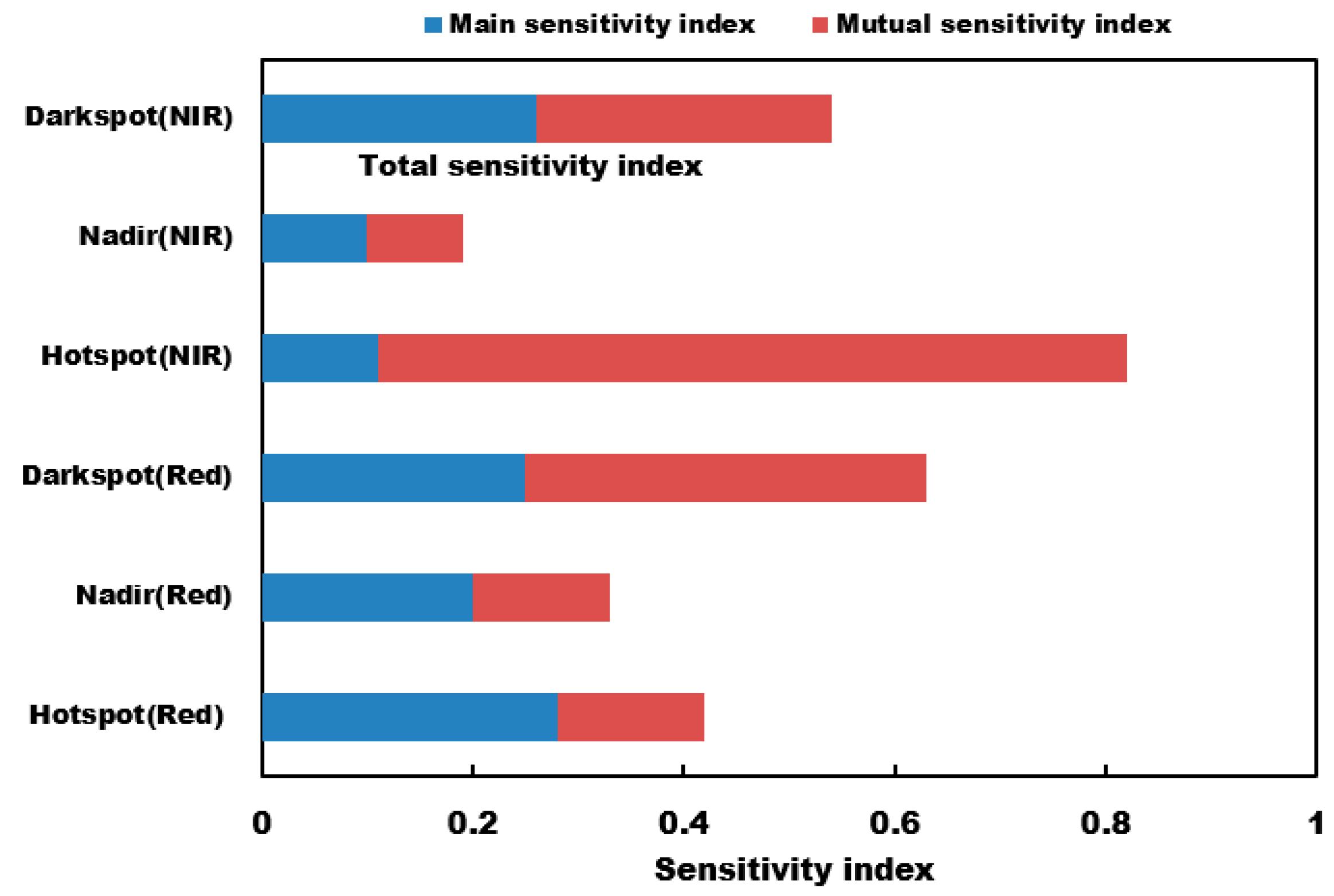
3.2.1. Sensitivity Analysis

The EFAST method has been developed based on the Fourier Amplitude Sensitivity Test (FAST) [76] and Sobol’s method [77] to estimate the contribution of the input parameters on the output by the model predictions variances, which are calculated from a decomposition of the Fourier-series representation. The total variances of the output (D) are given as follows:
D = i = 1 n D i + i = 1 n j = 1 j i n D i j + + D 1 , 2 , n ,
where Di is the variance of the output caused by input parameter Xi; Dij is the variance of the interaction between input parameters Xi and Xj; D1,2…n is the higher-order variance among multiple input parameters.
Three sensitivity indices can be calculated for each input parameter based on the above variances; i.e., the main (first-order) sensitivity index (Si), which is given in Equation (5), characterizes the contribution of a single input parameter to the output; the mutual (high-order) sensitivity index (Si…k) given in Equation (6) characterizes the interactions between a specific parameter and all other parameters; the total sensitivity index ( S i T ) is the sum of the above two parts (Equation (7)). Thus, this method considers not only individual input parameters but also the effect of the interaction between input parameters on the output.
S i = D i / D ,
S i k = D i j + D i j + 1 + D i k D ( j , k i ) ,
S i T = S i + j = 1 j i n S i j + + S 1 , 2 n .
In this study, we employed the EFAST method (Simlab2.2) and 4-scale model to analyze the sensitivity of the typical directional reflectances in the red and NIR bands to the variability of forest-canopy height, as shown in the processing workflow given in Figure 4.

3.2.2. Forest-Canopy Height Estimation

We used the RF regression-tree model to train the relationship between the LVIS-derived canopy heights and MODIS typical directional reflectances in the red and NIR bands; the model was then applied to estimate the forest-canopy heights. The processing workflow of canopy-height estimation from the typical directional reflectances is provided in Figure 4.
RF is a machine learning method that was proposed by Breiman [78] based on the classification-tree algorithm. RF runs by constructing multiple decision trees and randomly selecting training samples; it then outputs a mean prediction regression of the individual trees. Each decision tree is generated by the bootstrap-sampling method. The final predictions are determined by a majority vote of the trees. The RF package in the R language was used to implement the RF algorithm in this study.
The reflectances at typical observation angles (hotspot, darkspot, and nadir) in the red and NIR bands were reconstructed using the MODIS BRDF parameter data based on the hotspot-revised kernel-driven linear BRDF model (RTCLSR). The values of C1 and C2 used in the RTCLSR model are the optimized values derived by Jiao et al. [68] from the Polarization and Directionality of the Earth’s Reflectances (POLDER) hotspot observations as prior knowledge. This strategy has been successfully used in the generation process of the global MODIS clumping-index product [17].
To ensure the independence of the LVIS canopy-height data used for training the RF prediction model and for validating the estimated results, the LVIS canopy-height validation data were not used in the model-training process. For example, we selected LVIS-derived canopy heights in the Howland Forest as reference data for validation, but we merely used the canopy-height data in the Bartlett and Harvard Forests to train the canopy-height prediction model. The training data and validation data used in this study are shown in Table 4.
In theory, the accuracy of the LiDAR-derived canopy height can be significantly affected by terrain slope [35,79], because the slope broadens the LiDAR waveform and introduces a bias in canopy-height estimation. Therefore, to reduce the slope-induced uncertainty for the LiDAR-derived canopy height as input in the model-training process, we used mainly the LVIS data with a slope < 10° to train the model for the canopy-height estimation, although we appropriately maintained steep-slope LVIS data to test the results and analyze its potential influence on the estimation accuracy in this study.

4. Results and Analysis

4.1. Sensitivity Analysis of the Typical Directional Reflectances to Canopy Height

Within the possible range of the 4-scale model input parameters shown in Table 3, we first used Simlab2.2 to generate 959 pseudo values as each variable input parameter to the 4-scale model (Table 3) and then to simulate typical directional reflectances in the red and NIR bands using the 4-scale model. With these reflectances generated by the 4-scale model as outputs in conjunction with the corresponding sampling values by the Simlab2.2 as inputs, we finally used the EFAST method to analyze the sensitivity of the typical directional reflectances to forest canopy height.
Figure 5 depicts the EFAST sensitivity profiles of the main, mutual, and total sensitivity indices between the canopy height and the typical directional reflectances in the red and NIR bands. In general, the results present that the typical directional reflectances, especially in the direction of the hotspot and darkspot, show a higher sensitivity to canopy-height variations ( S i T > 0.2) than that in the nadir direction; on the contrary, the sensitivity of the reflectances in the nadir view directions to the canopy-height variation is the lowest among the three viewing angles in both bands.
The sensitivity of these reflectances to canopy height is somewhat different in the red and NIR bands (Figure 5) because the anisotropic reflectance patterns related to vegetation structural characteristics also depend on spectral bands, known as the BRDF spectral effects [60,61], at different spatial resolutions [80,81]. In the red band, the small leaf transmittance results in low multiple-scattering effects within the canopy and generates high reflectance anisotropy for the vegetation canopy. This makes the anisotropic reflectance in the red band more sensitive to the variability in vegetation canopy structures than that in the NIR band. Conversely, the high leaf transmittance in the NIR band leads to strong multiple-scattering effects and decreases the reflectance anisotropy, which therefore makes the reflectance in the NIR band less sensitive to vegetation canopy structure in theory than that in the red band. In conformity with the theoretical analysis, Figure 5 shows that the main sensitivity index of directional reflectances in the red band to the canopy height is generally higher than that in the NIR band. However, the main sensitivity index does not show much difference in darkspot reflectance (Figure 5), which may be attributed to the fact that the information regarding the canopy height in the shadows is not necessarily different between the red and NIR bands.
The mutual-sensitivity index indicates that the interactions among the forest canopy structure parameters (Table 3) on the typical directional reflectances also exhibit significant contributions to canopy height (Figure 5). Theoretically, vegetation canopy reflectances are affected by various canopy structures, e.g., LAI and canopy-coverage fraction. In the NIR band, multiple scattering effects are usually tightly related to the density of green leaves within the canopy that are quantified by the LAI, and more green leaves will generate more multiple scatterings within the canopy. This indicates that vegetation structures are mutually dependent on each other within the canopy, and the anisotropic reflectance patterns of vegetation canopy are usually the result of the common effects of various structural parameters. Figure 5 shows that the value of the mutual sensitivity index of the hotspot reflectance in the NIR band is the largest ( S i k ( j , k i ) = 0.71), which in turn causes the hotspot reflectance in the NIR band to have the largest total sensitivity index value ( S i T = 0.82) to the canopy height. This is apparently because of the most pronounced reflectance values in the hotspot direction in the NIR band. In comparison, the mutual-sensitivity index in the red band is substantially smaller than that in the NIR band, most likely due to the overall low reflectance in the red band.
As a summary, following the EFAST sensitivity analysis results, we can conclude that the directional reflectances in the hotspot and darkspot directions are more sensitive to canopy height than in the nadir direction (i.e., S i T for hotspot and darkspot reflectances both exceed 0.4, Figure 5). Therefore, the reflectances in the direction of the hotspot and darkspot are probably more helpful in the canopy-height estimation in terms of this sensitivity investigation.

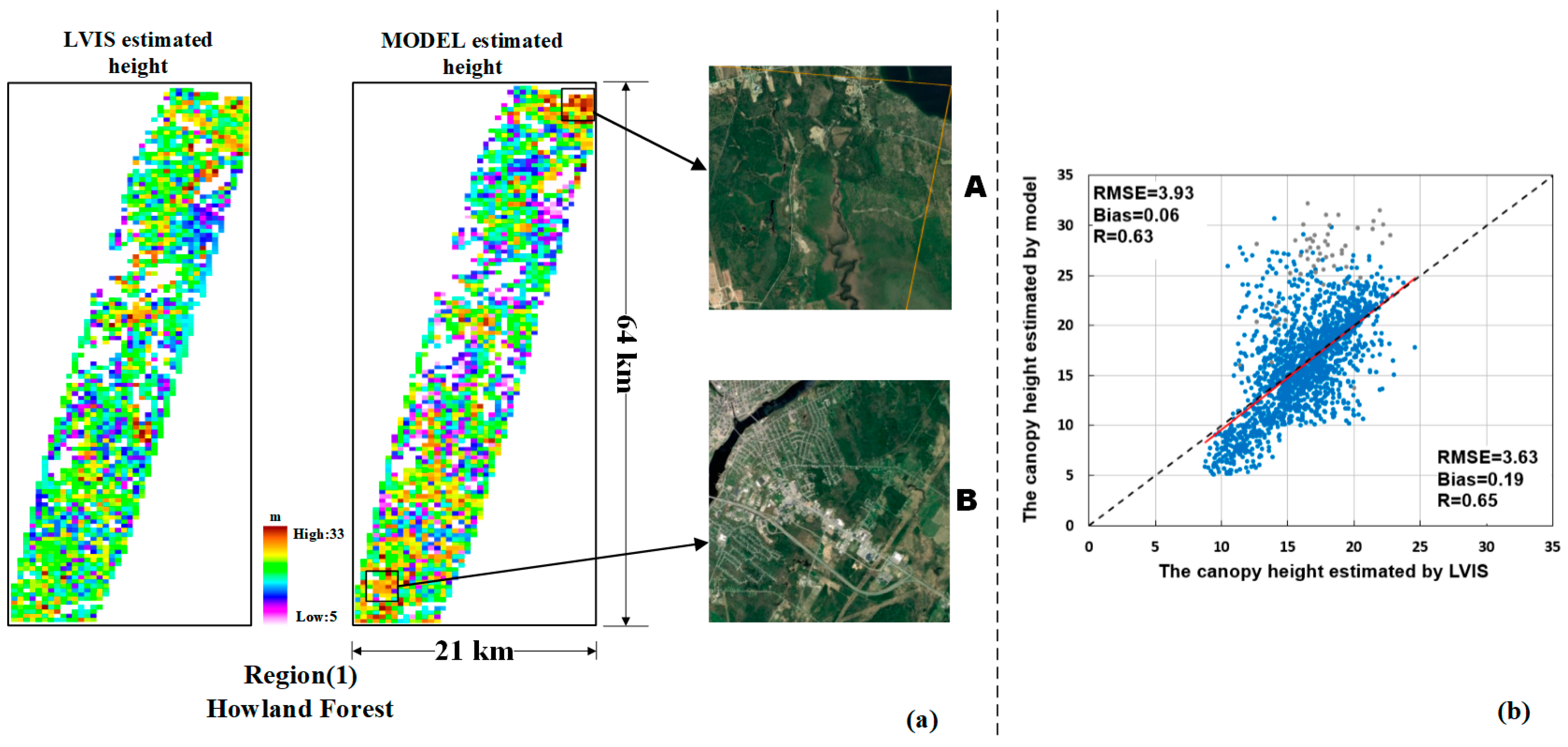
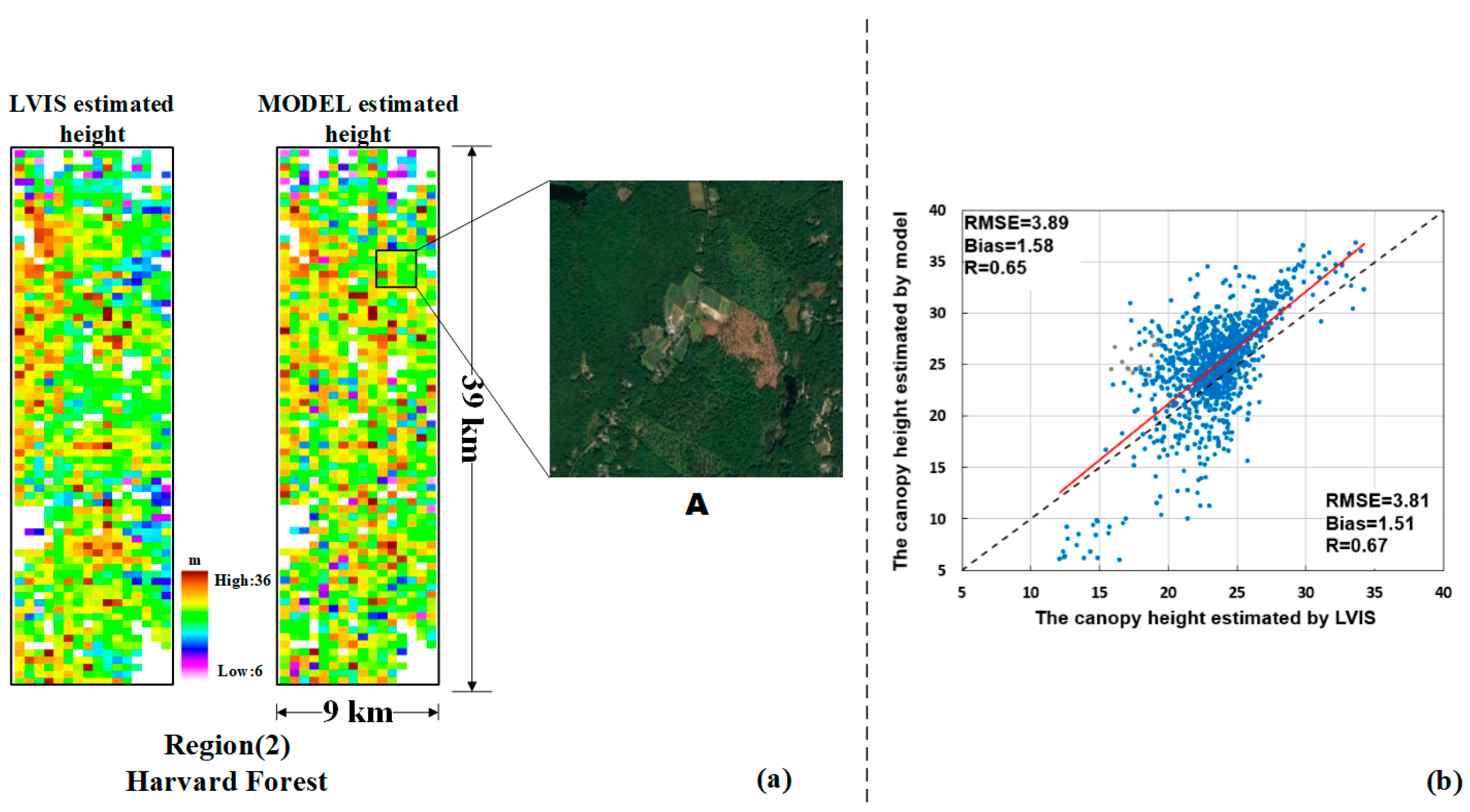
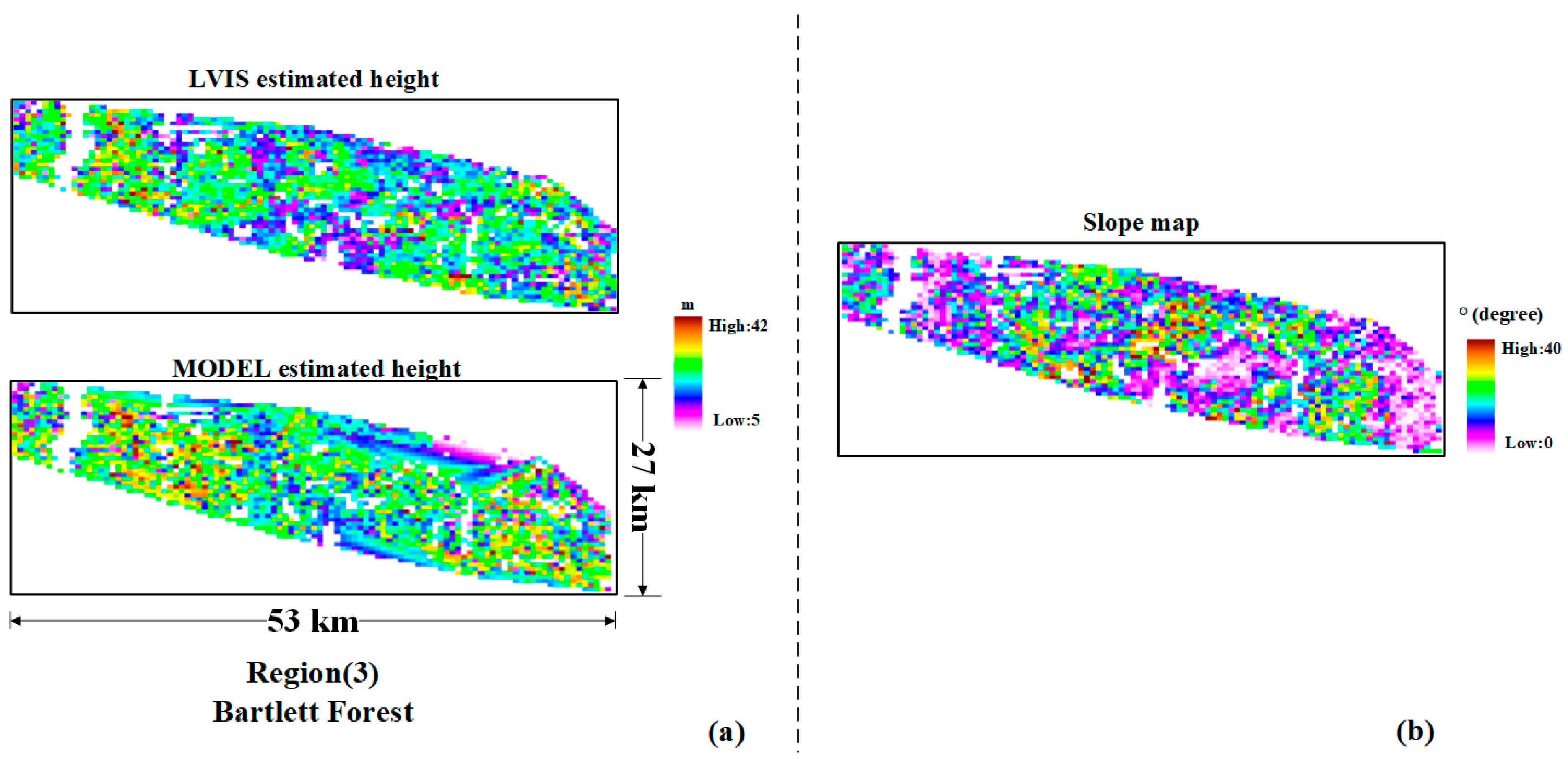
4.2. Canopy-Height Estimation and Validation

Canopy-height maps with a spatial resolution of 500 m over three large areas at the Howland Forest, Bartlett Forest, and Harvard Forest were produced to verify the ability of typical directional reflectances as inputs to estimate canopy height. The training and validation data used in this Section refer to Table 4. In general, the estimated canopy-height maps for these three large areas (Figure 6, Figure 7 and Figure 8) based on this proposed method show visually consistent spatial patterns with the LVIS-derived canopy heights; this verifies the feasibility of this method in canopy-height estimation.
More specifically, Figure 6a presents the comparison of the LVIS-derived canopy heights with the predicted canopy heights at 500 m resolution in the Howland Forest over an area of 64 × 21 km2. The correlation coefficient between the model-estimated canopy heights and LVIS-derived canopy heights is ~0.63, indicating a relatively high correlation. The RMSE is 3.93 m, accounting for ~25% relative errors in this study area (Figure 6b). A bias = 0.06 is almost negligible. In general, this result demonstrates a relatively high mapping accuracy based on this proposed method. Close examination of Figure 6a reveals some differences between the two maps of the LVIS-derived and model-estimated canopy heights. Obviously, the model-estimated canopy-height values are somewhat larger than the LVIS extracted canopy-height values, especially at both ends of the areas that are already marked by two black rectangles. Further examination of these two regions, A and B as individual examples (Figure 6a), with Google Maps, shows that these two areas are dominated by some mixed MODIS pixels, including lakes, rivers, and residential areas that are misclassified as forests in the MODIS land-cover product. The corresponding pixels in the scatter plot shown in Figure 6b are marked by gray points. Once such outliers are removed in regions A and B (gray spots shown in Figure 6b), the results have a somewhat improved prediction accuracy with a correlation coefficient of ~0.65 and RMSE of ~3.63 m. This analysis indicates that the uncertainty caused by the land-cover type map, particularly for some mixed pixels, is probably a main error source in the canopy-height estimation using the proposed method in this study.
We then analyzed another large area in the Harvard Forest. This region covers approximately 39 × 9 km2 (Figure 7a). The mapping results in Figure 7a show that the model-estimated canopy heights have very consistent spatial patterns with the LVIS-derived canopy heights. Similar to Figure 6, the statistical evaluation results are further provided for this area, which have good agreement between the LVIS-derived and model-estimated canopy heights with a correlation coefficient of ~0.65. The RMSE is 3.89 m, accounting for ~17% relative error (Figure 7b). The bias is 1.58 m. In general, this result further demonstrates the feasibility and reliability of this proposed method. Notably, some prominent outliers still exist in this mapping region, as shown in Figure 7b, and thus it needs a close investigation, as shown in Figure 7a. We found that mixed pixels are again the main error source in this mapping region. As an example, we examined some pixels in region A (Figure 7a), including not only trees but also farmland, buildings, and bare land, which are generally labeled as forests in the MODIS land-cover product. Once we removed these outliers from region A (gray spots in Figure 7b), the results were somewhat improved, with correlation coefficients reaching 0.67, the RMSE reducing to 3.81 m, and the bias decreasing to 1.51 m. Obviously, a better result is expected if such low-quality land-cover pixels are masked out through the use of a high-resolution land-cover map.
Finally, the proposed method was applied to the mountainous Bartlett Forest with an area of approximately 27 × 53 km2 (Figure 8a). In this study area, the total correlation coefficient and the RMSE between LVIS-derived and model-estimated canopy heights are ~0.48 and ~6.35 m (Figure 9a), respectively, without taking the effects of terrain into account. Compared with the previous two results of the Howland and Harvard forests, the result accuracy in this region is very challenging. To examine this result, we investigated the slope map in this study area (Figure 8b); it shows that the terrain in this study region is relatively complex with average and maximum slopes of 11.18° and 39.39°, respectively. The terrain effect in this study area is completely different from the first two study areas. Therefore, the influence of topographic factors on the canopy-height estimation in this region must be emphasized and further analyzed. Our specific statistics show that over 50% of the forest-covered pixels in this region are located in areas with slopes greater than 10°.
Figure 10 shows that the LVIS-extracted canopy height has a generally smaller value range (i.e., ~15–31 m) than the model-estimated canopy height (i.e., ~7–35 m), indicating that the LVIS signals are relatively insensitive to canopy-height variations in this mountainous region due to the topographic effects. However, the model-estimated canopy height tends to be overestimated in a larger range of the canopy-height values (e.g., >27 m), but tends to be underestimated in a smaller range of the canopy-height values (e.g., <15 m), compared to the LVIS-extracted canopy height. Once these pixels with steep slopes (slope >10°) were excluded from this map, the validation results greatly improved, with a correlation coefficient and RMSE of ~0.67 and ~5.78 m, respectively (Figure 9b). Obviously, the relatively large RMSE (i.e., ~5.78 m) in this mountainous area indicates that even a relatively small slope (e.g., 5–10°) probably has a relatively large influence on canopy-height estimation. Somewhat surprisingly, the terrain effect does not seem to largely influence the bias, most likely because the bias is offset by the overestimation and underestimation of the canopy heights in this case study.

5. Discussion

For the first time, the typical directional reflectances in the hotspot, nadir, and darkspot directions have been comprehensively tested to estimate forest-canopy height in conjunction with LiDAR signals in several selected study regions. The results indicated that multiangle reflectances in the hotspot, darkspot, and nadir directions contain important information about forest-canopy heights and therefore can be used as an effective data source to estimate forest-canopy height.
In the BRDF sampling capability of the MODIS sensors, typical reflectances are usually difficult to directly observe in most cases, particularly for the hotspot effect. To address this issue, we reconstructed the typical reflectances in the three viewing angles of the hotspot, nadir, and darkspot directions using the operational high-quality MODIS BRDF parameter product (i.e., MCD43A1) based on the RTCLSR model. The RTCLSR model is a hotspot-adjusted version of the kernel-driven RTLSR BRDF model that can accurately capture hotspot signatures by using two adjustable hotspot parameters (C1 and C2). The optimized values of the C1 and C2 parameters in the RTCLSR model that were derived from the 6 × 7 km POLDER hotspot observations in the previous study [68] were directly used as prior knowledge to reconstruct the 500 m MODIS multiangle reflectances. Obviously, the accuracy of these reconstructed typical reflectances is closely related to the robustness of the kernel-driven model. As is well known, the reconstructed reflectances from MODIS multiangle observations have been widely used in many fields, e.g., derivation of the MODIS global-land-cover products [82], improvement of the accuracy of various land-surface-classification schemes [83,84], and estimation of the structural parameters of vegetation canopies [17,64]; however, the potential uncertainty caused by such typical reflectances through use of the RTCLSR model must be considered and discussed, particularly for the pixel-size difference in hotspot signatures between the MODIS and POLDER sensors at two very different spatial resolutions [72,81].
In addition, in this study, the relatively coarse spatial resolution of MODIS data is definitely an inevitable error source, introducing various uncertainties in the tree-height retrievals, especially by the mixed pixels from the MODIS land-cover product. This study shows that some pixels that are identified as of forest type in the MODIS land-cover product are actually mixed pixels that cover the forest, roads, and water. These mixed pixels tend to have a low prediction accuracy of tree-canopy heights, resulting in a significant bias in the process of tree-height estimations. Indeed, the mixed pixels were previously reported as a strong limitation factor, especially in utilizing coarse-resolution satellite images to monitor vegetation dynamics [85]. Similarly, this study further confirms that the effect of mixed pixels deserves much more attention in the study of canopy-height estimation, as shown in Figure 6 and Figure 7.
Finally, the terrain slope is another important factor determined here to have a large effect on tree-height retrievals. As shown in Figure 9, this study generally performs well in low-to-moderate slope areas (i.e., slope <10°), but the results get worse in mountainous study regions with relatively steep slopes. Indeed, previous studies noted that the topographic factors had a large influence not only on the BRDF patterns [86,87,88,89] but also on the accuracy of the LiDAR-derived canopy height [35,79], which is, in turn, usually used as the true value to train the canopy-height prediction model and/or to validate the predicted results in such studies. Therefore, we must be aware of the potential uncertainty caused by a steep terrain slope not only for using the multiangle reflectances but also for deriving the LVIS-derived canopy height in such studies.
Despite the various uncertainties mentioned above, we must realize that the multiangle reflectances, even in just the three typical directions of the hotspot, nadir, and darkspot being explored here, contain important information regarding canopy heights, and therefore are generally helpful in the retrievals of canopy heights in conjunction with the corresponding land-cover data.

6. Conclusions

Forest-canopy height is an important parameter for the estimations of forest biomass and terrestrial carbon flux that are in turn essential to climate-change research at regional and global scales. In this study, the potential of using three typical directional reflectances (i.e., reflectances obtained from the hotspot, darkspot, and nadir directions) to estimate forest canopy height was comprehensively explored based on the LVIS-extracted canopy-height data in the Howland Forest, Harvard Forest, and mountainous Bartlett Forest. This study highlights several conclusive results as follows:
(1) The reflectances in the off-nadir viewing directions are generally sensitive to canopy height variations in terms of the sensitivity analysis using the 4-scale model simulations.
(2) Generally, a relatively high-accuracy canopy height could be retrieved by using three typical directional reflectances (i.e., hotspot, nadir, and darkspot) in conjunction with corresponding land-cover data in the three study areas. Specifically, the correlation coefficients (R) and RMSE between the modeled canopy height and the LVIS-derived canopy height arrive at 0.63 and 3.93 m for the Howland Forest; 0.65 and 3.89 m for the Harvard Forest; 0.48 and 6.60 m for the mountainous Bartlett Forest. Such results are generally comparable to the previous studies using various auxiliary input data [42,43,44]. The results can be significantly improved if mixed pixels or pixels with a steep slope (e.g., slope >10°) are examined and excluded.
(3) The MODIS multiangle reflectances at the three typical viewing angles show the potential to estimate forest-canopy height in conjunction with corresponding land-cover data. However, the problem of mixed pixels and large terrain slope pixels are still a challenge and need more research, particularly in conjunction with using high-resolution land cover classification maps in the near future.

Author Contributions

Conceptualization, L.C. and Z.J.; data curation, L.C., Y.D., S.Y., A.D., and Y.C.; formal analysis, L.C., Z.J., Y.D., and X.Z.; funding acquisition, Z.J.; software, L.C., Y.D., and M.S.; writing—original draft, L.C.; writing—review & editing, Z.J., Y.D., M.S., X.Z., J.G., and R.X.

Funding

This work was supported by the National Natural Science Foundation of China (Nos. 41571326 and 41801237). The LVIS data sets were provided by the Laser Vegetation Imaging Sensor (LVIS) team in the Laser Remote Sensing Branch at the NASA Goddard Space Flight Center with support from the University of Maryland, College Park. Funding for the collection and processing of the data from the northeastern U.S.A. was provided by NASA’s Terrestrial Ecology Program (NASA Grant number NAG512112).

Conflicts of Interest

The authors declare no conflict of interest.

References

  1. Lefsky, M.A.; Harding, D.J.; Keller, M.; Cohen, W.B.; Carabajal, C.C.; Espirito-Santo, F.D.; Hunter, M.O.; de Oliveira, R. Estimates of Forest Canopy Height and Aboveground Biomass Using ICESat. Geophys. Res. Lett. 2005, 32. [Google Scholar] [CrossRef]
  2. Zhang, G.; Ganguly, S.; Nemani, R.R.; White, M.A.; Milesi, C.; Hashimoto, H.; Wang, W.; Saatchi, S.; Yu, Y.; Myneni, R.B. Estimation of Forest Aboveground Biomass in California Using Canopy Height and Leaf Area Index Estimated From Satellite Data. Remote Sens. Environ. 2014, 151, 44–56. [Google Scholar] [CrossRef]
  3. Li, W.; Niu, Z.; Chen, H.; Li, D.; Wu, M.; Zhao, W. Remote Estimation of Canopy Height and Aboveground Biomass of Maize Using High-Resolution Stereo Images From a Low-Cost Unmanned Aerial Vehicle System. Ecol. Indic. 2016, 67, 637–648. [Google Scholar] [CrossRef]
  4. Coomes, D.A.; Flores, O.; Holdaway, R.; Jucker, T.; Lines, E.R.; Vanderwel, M.C. Wood Production Response to Climate Change Will Depend Critically On Forest Composition and Structure. Glob. Chang. Biol. 2014, 20, 3632–3645. [Google Scholar] [CrossRef] [PubMed]
  5. Janowiak, M.K.; Webster, C.R. Promoting Ecological Sustainability in Woody Biomass Harvesting. J. For. 2010, 108, 16–23. [Google Scholar]
  6. Masek, J.G.; Collatz, G.J. Estimating Forest Carbon Fluxes in a Disturbed Southeastern Landscape: Integration of Remote Sensing, Forest Inventory, and Biogeochemical Modeling. J. Geophys. Res. Biogeosci. 2006, 111. [Google Scholar] [CrossRef]
  7. Li, X.W.; Straher, A.H. Geometric-Optical Bidirectional Reflectance Modeling of the Discrete Crown Vegetation Canopy—Effect of Crown Shape and Mutual Shadowing. IEEE Trans. Geosci. Remote Sens. 1992, 30, 276–292. [Google Scholar] [CrossRef]
  8. Chen, J.M.; Leblanc, S.G. A Four-Scale Bidirectional Reflectance Model Based On Canopy Architecture. IEEE Trans. Geosci. Remote Sens. 1997, 35, 1316–1337. [Google Scholar] [CrossRef]
  9. Tang, S.; Chen, J.M.; Zhu, Q.; Li, X.; Chen, M.; Sun, R.; Zhou, Y.; Deng, F.; Xie, D. LAI Inversion Algorithm Based On Directional Reflectance Kernels. J. Environ. Manag. 2007, 85, 638–648. [Google Scholar] [CrossRef]
  10. Simic, A.; Chen, J.M.; Freemantle, J.R.; Miller, J.R.; Pisek, J. Improving Clumping and LAI Algorithms Based on Multiangle Airborne Imagery and Ground Measurements. IEEE Trans. Geosci. Remote Sens. 2010, 48, 1742–1759. [Google Scholar] [CrossRef]
  11. Yang, G.; Zhao, C.; Liu, Q.; Huang, W.; Wang, J. Inversion of a Radiative Transfer Model for Estimating Forest LAI From Multisource and Multiangular Optical Remote Sensing Data. IEEE Trans. Geosci. Remote Sens. 2011, 49, 988–1000. [Google Scholar] [CrossRef]
  12. Ma, H.; Song, J.; Wang, J.; Xiao, Z.; Fu, Z. Improvement of Spatially Continuous Forest LAI Retrieval by Integration of Discrete Airborne LiDAR and Remote Sensing Multi-Angle Optical Data. Agric. For. Meteorol. 2014, 189, 60–70. [Google Scholar] [CrossRef]
  13. Knyazikhin, Y.; Martonchik, J.V.; Myneni, R.B.; Diner, D.J.; Running, S.W. Synergistic Algorithm for Estimating Vegetation Canopy Leaf Area Index and Fraction of Absorbed Photosynthetically Active Radiation from MODIS and MISR Data. J. Geophys. Res. Atmos. 1998, 103, 32257–32275. [Google Scholar] [CrossRef]
  14. Chen, J.M.; Menges, C.H.; Leblanc, S.G. Global Mapping of Foliage Clumping Index Using Multi-Angular Satellite Data. Remote Sens. Environ. 2005, 97, 447–457. [Google Scholar] [CrossRef]
  15. He, L.; Chen, J.M.; Pisek, J.; Schaaf, C.B.; Strahler, A.H. Global Clumping Index Map Derived From the MODIS BRDF Product. Remote Sens. Environ. 2012, 119, 118–130. [Google Scholar] [CrossRef]
  16. Hill, M.J.; Roman, M.O.; Schaaf, C.B.; Hutley, L.; Brannstrom, C.; Etter, A.; Hanan, N.P. Characterizing Vegetation Cover in Global Savannas with an Annual Foliage Clumping Index Derived From the MODIS BRDF Product. Remote Sens. Environ. 2011, 115, 2008–2024. [Google Scholar] [CrossRef]
  17. Jiao, Z.; Dong, Y.; Schaaf, C.B.; Chen, J.M.; Román, M.; Wang, Z.; Zhang, H.; Ding, A.; Erb, A.; Hill, M.J.; et al. An Algorithm for the Retrieval of the Clumping Index (CI) From the MODIS BRDF Product Using an Adjusted Version of the Kernel-Driven BRDF Model. Remote Sens. Environ. 2018, 209, 594–611. [Google Scholar] [CrossRef]
  18. Leblanc, S.G.; Chen, J.M.; White, H.P.; Latifovic, R.; Lacaze, R.; Roujean, J. Canada-Wide Foliage Clumping Index Mapping From Multiangular POLDER Measurements. Can. J. Remote Sens. 2005, 31, 364–376. [Google Scholar] [CrossRef]
  19. Pisek, J.; Chen, J.M.; Lacaze, R.; Sonnentag, O.; Alikas, K. Expanding Global Mapping of the Foliage Clumping Index with Multi-Angular POLDER Three Measurements: Evaluation and Topographic Compensation. ISPRS J. Photogramm. 2010, 65, 341–346. [Google Scholar] [CrossRef]
  20. Pisek, J.; Chen, J.M.; Nilson, T. Estimation of Vegetation Clumping Index Using MODIS BRDF Data. Int. J. Remote Sens. 2011, 32, 2645–2657. [Google Scholar] [CrossRef]
  21. Pisek, J.; Ryu, Y.; Sprintsin, M.; He, L.; Oliphant, A.J.; Korhonen, L.; Kuusk, J.; Kuusk, A.; Bergstrom, R.; Verrelst, J.; et al. Retrieving Vegetation Clumping Index from-Multi-angle Imaging SpectroRadiometer (MISR) Data at 275 M Resolution. Remote Sens. Environ. 2013, 138, 126–133. [Google Scholar] [CrossRef]
  22. Wei, S.; Fang, H. Estimation of Canopy Clumping Index From MISR and MODIS Sensors Using the Normalized Difference Hotspot and Darkspot (NDHD) Method: The Influence of BRDF Models and Solar Zenith Angle. Remote Sens. Environ. 2016, 187, 476–491. [Google Scholar] [CrossRef]
  23. Zhu, G.; Ju, W.; Chen, J.M.; Gong, P.; Xing, B.; Zhu, J. Foliage Clumping Index Over China’s Landmass Retrieved From the MODIS BRDF Parameters Product. IEEE Trans. Geosci. Remote Sens. 2012, 50, 2122–2137. [Google Scholar] [CrossRef]
  24. Chopping, M.; Schaaf, C.B.; Zhao, F.; Wang, Z.; Nolin, A.W.; Moisen, G.G.; Martonchik, J.V.; Bull, M. Forest Structure and Aboveground Biomass in the Southwestern United States From MODIS and MISR. Remote Sens. Environ. 2011, 115, 2943–2953. [Google Scholar] [CrossRef]
  25. Wang, Z.; Schaaf, C.B.; Lewis, P.; Knyazikhin, Y.; Schull, M.A.; Strahler, A.H.; Yao, T.; Myneni, R.B.; Chopping, M.J.; Blair, B.J. Retrieval of Canopy Height Using Moderate-Resolution Imaging Spectroradiometer (MODIS) Data. Remote Sens. Environ. 2011, 115, 1595–1601. [Google Scholar] [CrossRef]
  26. Heiskanen, J. Tree Cover and Height Estimation in the Fennoscandian Tundra–Taiga Transition Zone Using Multiangular MISR Data. Remote Sens. Environ. 2006, 103, 97–114. [Google Scholar] [CrossRef]
  27. Justice, C.O.; Vermote, E.; Townshend, J.R.G.; Defries, R.; Roy, D.P. The Moderate Resolution Imaging Spectroradiometer (MODIS): Land Remote Sensing for Global Change Research. IEEE Trans. Geosci. Remote Sens. 1998, 36, 1228–1248. [Google Scholar] [CrossRef]
  28. Diner, D.J.; Beckert, J.C.; Reilly, T.H.; Bruegge, C.J.; Conel, J.E.; Ralph, A.; Kahn, J.V.M. Multi-Angle Imaging SpectroRadiometer (MISR) Instrument Description and Experiment Overview. IEEE Trans. Geosci. Remote Sens. 1998, 36, 1072–1087. [Google Scholar] [CrossRef]
  29. Lefsky, M.A.; Harding, D.; Cohen, W.B.; Parker, G.; Shugart, H.H. Surface Lidar Remote Sensing of Basal Area and Biomass in Deciduous Forests of Eastern Maryland, USA. Remote Sens. Environ. 1999, 67, 83–98. [Google Scholar] [CrossRef]
  30. Lim, K.; Treitz, P.; Wulder, M.; St-Onge, B.; Flood, M. LiDAR Remote Sensing of Forest Structure. Prog. Phys. Geog. 2003, 27, 88–106. [Google Scholar] [CrossRef]
  31. Kimes, D.S.; Ranson, K.J.; Sun, G.; Blair, J.B. Predicting Lidar Measured Forest Vertical Structure From Multi-Angle Spectral Data. Remote Sens. Environ. 2006, 100, 503–511. [Google Scholar] [CrossRef]
  32. Anderson, J.; Martin, M.E.; Smith, M.; Dubayah, R.O.; Hofton, M.A.; Hyde, P.; Peterson, B.E.; Blair, J.B.; Knox, R.G. The Use of Waveform Lidar to Measure Northern Temperate Mixed Conifer and Deciduous Forest Structure in New Hampshire. Remote Sens. Environ. 2006, 105, 248–261. [Google Scholar] [CrossRef]
  33. Brilli, L.; Chiesi, M.; Brogi, C.; Magno, R.; Arcidiaco, L.; Bottai, L.; Tagliaferri, G.; Bindi, M.; Maselli, F. Combination of Ground and Remote Sensing Data to Assess Carbon Stock Changes in the Main Urban Park of Florence. Urban For. Urban Green. 2019, 43, 126377. [Google Scholar] [CrossRef]
  34. Rahman, M.T.; Rashed, T. Urban Tree Damage Estimation Using Airborne Laser Scanner Data and Geographic Information Systems: An Example From 2007 Oklahoma Ice Storm. Urban For. Urban Green. 2015, 14, 562–572. [Google Scholar] [CrossRef]
  35. Lefsky, M.A.; Keller, M.; Pang, Y.; de Camargo, P.B.; Hunter, M.O. Revised Method for Forest Canopy Height Estimation From Geoscience Laser Altimeter System Waveforms. J. Appl. Remote Sens. 2007, 1, 013537. [Google Scholar] [CrossRef]
  36. Lefsky, M.A. A Global Forest Canopy Height Map From the Moderate Resolution Imaging Spectroradiometer and the Geoscience Laser Altimeter System. Geophys. Res. Lett. 2010, 37, 78–82. [Google Scholar] [CrossRef]
  37. Simard, M.; Pinto, N.; Fisher, J.B.; Baccini, A. Mapping Forest Canopy Height Globally with Spaceborne Lidar. J. Geophys. Res. Biogeosci. 2011, 116. [Google Scholar] [CrossRef]
  38. Wang, Y.; Li, G.; Ding, J.; Guo, Z.; Tang, S.; Wang, C.; Huang, Q.; Liu, R.; Chen, J.M. A Combined GLAS and MODIS Estimation of the Global Distribution of Mean Forest Canopy Height. Remote Sens. Environ. 2016, 174, 24–43. [Google Scholar] [CrossRef]
  39. Stojanova, D.; Panov, P.; Gjorgjioski, V.; Kohler, A.; Dzeroski, S. Estimating Vegetation Height and Canopy Cover From Remotely Sensed Data with Machine Learning. Ecol. Inform. 2010, 5, 256–266. [Google Scholar] [CrossRef]
  40. Cartus, O.; Kellndorfer, J.; Rombach, M.; Walker, W. Mapping Canopy Height and Growing Stock Volume Using Airborne Lidar, ALOS PALSAR and Landsat ETM. Remote Sens. 2012, 4, 3320–3345. [Google Scholar] [CrossRef]
  41. Ahmed, O.S.; Franklin, S.E.; Wulder, M.A.; White, J.C. Characterizing Stand-Level Forest Canopy Cover and Height Using Landsat Time Series, Samples of Airborne LiDAR, and the Random Forest Algorithm. ISPRS J. Photogramm. 2015, 101, 89–101. [Google Scholar] [CrossRef]
  42. Ni, X.; Zhou, Y.; Cao, C.; Wang, X.; Shi, Y.; Park, T.; Choi, S.; Myneni, R.B. Mapping Forest Canopy Height over Continental China Using Multi-Source Remote Sensing Data. Remote Sens. 2015, 7, 8436–8452. [Google Scholar] [CrossRef] [Green Version]
  43. Huang, H.; Liu, C.; Wang, X.; Biging, G.S.; Chen, Y.; Yang, J.; Gong, P. Mapping Vegetation Heights in China Using Slope Correction ICESat Data, SRTM, MODIS-derived and Climate Data. ISPRS J. Photogramm. 2017, 129, 189–199. [Google Scholar] [CrossRef]
  44. Wang, M.; Sun, R.; Xiao, Z. Estimation of Forest Canopy Height and Aboveground Biomass from Spaceborne LiDAR and Landsat Imageries in Maryland. Remote Sens. 2018, 10, 344. [Google Scholar] [CrossRef]
  45. Cui, L.; Jiao, Z.; Dong, Y.; Zhang, X.; Sun, M.; Yin, S.; Chang, Y.; He, D.; Ding, A. Forest Vertical Structure From Modis Brdf Shape Indicators. In Proceedings of the 2018 IEEE International Symposium on Geoscience and Remote Sensing IGARSS, Valencia, Spain, 22–27 July 2018; pp. 5911–5914. [Google Scholar]
  46. Saltelli, A.; Tarantola, S.; Chan, K. A Quantitative Model-Independent Method for Global Sensitivity Analysis of Model Output. Technometrics 1999, 41, 39–56. [Google Scholar] [CrossRef]
  47. The University of Maine. Available online: https://umaine.edu/howlandforest/ (accessed on 10 July 2018).
  48. United States Department of Agriculture. Available online: https://www.nrs.fs.fed.us/ef/locations/nh/bartlett/ (accessed on 10 July 2018).
  49. Blair, J.B.; Rabine, D.L.; Hofton, M.A. The Laser Vegetation Imaging Sensor: A Medium-Altitude, Digitisation-Only, Airborne Laser Altimeter for Mapping Vegetation and Topography. ISPRS J. Photogramm. 1999, 54, 115–122. [Google Scholar] [CrossRef]
  50. Hancock, S.; Armston, J.; Hofton, M.; Sun, X.; Tang, H.; Duncanson, L.I.; Kellner, J.R.; Dubayah, R. The GEDI Simulator: A Large-Footprint Waveform Lidar Simulator for Calibration and Validation of Spaceborne Missions. Earth Space Sci. 2019, 10, 294–310. [Google Scholar] [CrossRef] [PubMed]
  51. Schaaf, C.B.; Gao, F.; Strahler, A.H.; Lucht, W.; Li, X.; Tsang, T.; Strugnell, N.C.; Zhang, X.; Jin, Y.; Muller, J.; et al. First Operational BRDF, Albedo Nadir Reflectance Products From MODIS. Remote Sens. Environ. 2002, 83, 135–148. [Google Scholar] [CrossRef]
  52. Wang, Z.; Schaaf, C.B.; Sun, Q.; Shuai, Y.; Roman, M.O. Capturing Rapid Land Surface Dynamics with Collection V006 MODIS BRDF/NBAR/Albedo (MCD43) Products. Remote Sens. Environ. 2018, 207, 50–64. [Google Scholar] [CrossRef]
  53. Hansen, M.C.; DeFries, R.S.; Townshend, J.R.G.; Carroll, M.; Dimiceli, C.; Sohlberg, R.A. Global Percent Tree Cover at a Spatial Resolution of 500 Meters: First Results of the MODIS Vegetation Continuous Fields Algorithm. Earth Interact. 2003, 7, 1–15. [Google Scholar] [CrossRef] [Green Version]
  54. Friedl, M.A.; Sulla-Menashe, D.; Tan, B.; Schneider, A.; Ramankutty, N.; Sibley, A.; Huang, X. MODIS Collection 5 Global Land Cover: Algorithm Refinements and Characterization of New Datasets. Remote Sens. Environ. 2010, 114, 168–182. [Google Scholar] [CrossRef]
  55. Farr, T.G.; Rosen, P.A.; Caro, E.; Crippen, R.; Duren, R.; Hensley, S.; Kobrick, M.; Paller, M.; Rodriguez, E.; Roth, L.; et al. The Shuttle Radar Topography Mission. Rev. Geophys. 2007, 45. [Google Scholar] [CrossRef] [Green Version]
  56. Wang, Z.; Schaaf, C.B.; Chopping, M.J.; Strahler, A.H.; Wang, J.; Roman, M.O.; Rocha, A.V.; Woodcock, C.E.; Shuai, Y. Evaluation of Moderate-resolution Imaging Spectroradiometer (MODIS) Snow Albedo Product (MCD43A) Over Tundra. Remote Sens. Environ. 2012, 117, 264–280. [Google Scholar] [CrossRef]
  57. Wang, Z.; Schaaf, C.B.; Strahler, A.H.; Chopping, M.J.; Roman, M.O.; Shuai, Y.; Woodcock, C.E.; Hollinger, D.Y.; Fitzjarrald, D.R. Evaluation of MODIS Albedo Product (MCD43A) Over Grassland, Agriculture and Forest Surface Types During Dormant and Snow-Covered Periods. Remote Sens. Environ. 2014, 140, 60–77. [Google Scholar] [CrossRef]
  58. Beck, P.; Atzberger, C.; Hogda, K.A.; Johansen, B.; Skidmore, A.K. Improved Monitoring of Vegetation Dynamics at Very High Latitudes: A New Method Using MODIS NDVI. Remote Sens. Environ. 2006, 100, 321–334. [Google Scholar] [CrossRef]
  59. Baret, F.; Clevers, J.; Steven, M.D. The Robustness of Canopy Gap Fraction Estimates from Red and Near-Infrared Reflectances—A Comparison of Approaches. Remote Sens. Environ. 1995, 54, 141–151. [Google Scholar] [CrossRef]
  60. Luquet, D.; Begue, A.; Dauzat, J.; Nouvellon, Y.; Rey, H. Effect of the Vegetation Clumping On the BRDF of a Semi-Arid Grassland: Comparison of the SAIL Model and Ray Tracing Method Applied to a 3D Computerized Vegetation Canopy. In Proceedings of the 1998 IEEE International Symposium on Geoscience and Remote Sensing (IGARSS), Seattle, WA, USA, 6–10 July 1998; pp. 791–793. [Google Scholar]
  61. Hall, F.G.; Shimabukuro, Y.E.; Huemmrich, K.F. Remote-Sensing of Forest Biophysical Structure Using Mixture Decomposition and Geometric Reflectance Models. Ecol. Appl. 1995, 5, 993–1013. [Google Scholar] [CrossRef]
  62. Jiao, Z.; Hill, M.J.; Schaaf, C.B.; Zhang, H.; Wang, Z.; Li, X. An Anisotropic Flat Index (AFX) to Derive BRDF Archetypes From MODIS. Remote Sens. Environ. 2014, 141, 168–187. [Google Scholar] [CrossRef]
  63. Gao, F.; Schaaf, C.B.; Strahler, A.H.; Jin, Y.; Li, X. Detecting Vegetation Structure Using a Kernel-Based BRDF Model. Remote Sens. Environ. 2003, 86, 198–205. [Google Scholar] [CrossRef]
  64. Zhang, H.; Jiao, Z.; Chen, L.; Dong, Y.; Zhang, X.; Lian, Y.; Qian, D.; Cui, T. Quantifying the Reflectance Anisotropy Effect On Albedo Retrieval From Remotely Sensed Observations Using Archetypal BRDFs. Remote Sens. 2018, 10, 1628. [Google Scholar] [CrossRef]
  65. Chen, J.M.; Leblanc, S.G. Multiple-Scattering Scheme Useful for Geometric Optical Modeling. IEEE Trans. Geosci. Remote Sens. 2001, 39, 1061–1071. [Google Scholar] [CrossRef]
  66. Roujean, J.L.; Leroy, M.; Deschamps, P.Y. A Bidirectional Reflectance Model of the Earths Surface for the Correction of Remote-Sensing Data. J. Geophys. Res. Atmos. 1992, 97, 20455–20468. [Google Scholar] [CrossRef]
  67. Lucht, W.; Schaaf, C.B.; Strahler, A.H. An Algorithm for the Retrieval of Albedo From Space Using Semiempirical BRDF Models. IEEE Trans. Geosci. Remote Sens. 2000, 38, 977–998. [Google Scholar] [CrossRef]
  68. Jiao, Z.; Schaaf, C.B.; Dong, Y.; Roman, M.; Hill, M.J.; Chen, J.M.; Wang, Z.; Zhang, H.; Saenz, E.; Poudyal, R.; et al. A Method for Improving Hotspot Directional Signatures in BRDF Models Used for MODIS. Remote Sens. Environ. 2016, 186, 135–151. [Google Scholar] [CrossRef]
  69. Chen, J.M.; Cihlar, J. A Hotspot Function in a Simple Bidirectional Reflectance Model for Satellite Applications. J. Geophys. Res. Atmos. 1997, 102, 25907–25913. [Google Scholar] [CrossRef]
  70. Dong, Y.; Jiao, Z.; Yin, S.; Zhang, H.; Zhang, X.; Cui, L.; He, D.; Ding, A.; Chang, Y.; Yang, S. Influence of Snow On the Magnitude and Seasonal Variation of the Clumping Index Retrieved From MODIS BRDF Products. Remote Sens. 2018, 10, 1194. [Google Scholar] [CrossRef]
  71. Zhang, X.; Jiao, Z.; Dong, Y.; Zhang, H.; Li, Y.; He, D.; Ding, A.; Yin, S.; Cui, L.; Chang, Y. Potential Investigation of Linking PROSAIL with the Ross-Li BRDF Model for Vegetation Characterization. Remote Sens. 2018, 10, 437. [Google Scholar] [CrossRef]
  72. Dong, Y.; Jiao, Z.; Cui, L.; Zhang, H.; Zhang, X.; Yin, S.; Ding, A.; Chang, Y.; Xie, R.; Guo, J. Assessment of the Hotspot Effect for the PROSAIL Model with POLDER Hotspot Observations Based on the Hotspot-Enhanced Kernel-Driven BRDF Model. IEEE Trans. Geosci. Remote Sens. 2019, in press. [Google Scholar] [CrossRef]
  73. Jiao, Z.; Ding, A.; Kokhanovsky, A.; Schaaf, C.; Breon, F.; Dong, Y.; Wang, Z.; Liu, Y.; Zhang, X.; Yin, S.; et al. Development of a Snow Kernel to Better Model the Anisotropic Reflectance of Pure Snow in a Kernel-Driven BRDF Model Framework. Remote Sens. Environ. 2019, 221, 198–209. [Google Scholar] [CrossRef]
  74. Ding, A.; Jiao, Z.; Dong, Y.; Qu, Y.; Zhang, X.; Xiong, C.; He, D.; Yin, S.; Cui, L.; Chang, Y. An Assessment of the Performance of Two Snow Kernels in Characterizing Snow Scattering Properties. Int. J. Remote Sens. 2019, 40, 6315–6335. [Google Scholar] [CrossRef]
  75. Ding, A.; Jiao, Z.; Dong, Y.; Xi, X.; Zhang, X.; Xiong, C.; He, D.; Yin, S.; Cui, L.; Chang, Y. Evaluation of the Snow Albedo Retrieved from the Snow Kernel Improved the Ross-Roujean BRDF Model. Remote Sens. 2019, 11, 1611. [Google Scholar] [CrossRef]
  76. Cukier, R.I.; Fortuin, C.M.; Shuler, K.E.; Petschek, A.G.; Schaibly, J.H. Study of Sensitivity of Coupled Reaction Systems to Uncertainties in Rate Coefficients.1. Theory. J. Chem. Phys. 1973, 59, 3873–3878. [Google Scholar] [CrossRef]
  77. Sobol, I.M. Sensitivity Estimates for Nonlinear Mathematical Models. Math. Model. Comput. Exp. 1993, 1, 407–414. [Google Scholar]
  78. Breiman, L. Random Forests. Mach. Learn. 2001, 45, 5–32. [Google Scholar] [CrossRef] [Green Version]
  79. Wang, X.; Huang, H.; Gong, P.; Liu, C.; Li, C.; Li, W. Forest Canopy Height Extraction in Rugged Areas with ICESat/GLAS Data. IEEE Trans. Geosci. Remote Sens. 2014, 52, 4650–4657. [Google Scholar] [CrossRef]
  80. Roman, M.O.; Gatebe, C.K.; Schaaf, C.B.; Poudyal, R.; Wang, Z.; King, M.D. Variability in Surface BRDF at Different Spatial Scales (30 M-500 M) Over a Mixed Agricultural Landscape as Retrieved From Airborne and Satellite Spectral Measurements. Remote Sens. Environ. 2011, 115, 2184–2203. [Google Scholar] [CrossRef]
  81. Jiao, Z.; Zhang, X.; Breon, F.; Dong, Y.; Schaaf, C.B.; Roman, M.; Wang, Z.; Cui, L.; Yin, S.; Ding, A.; et al. The Influence of Spatial Resolution On the Angular Variation Patterns of Optical Reflectance as Retrieved From MODIS and POLDER Measurements. Remote Sens. Environ. 2018, 215, 371–385. [Google Scholar] [CrossRef]
  82. Friedl, M.A.; McIver, D.K.; Hodges, J.; Zhang, X.Y.; Muchoney, D.; Strahler, A.H.; Woodcock, C.E.; Gopal, S.; Schneider, A.; Cooper, A.; et al. Global Land Cover Mapping From MODIS: Algorithms and Early Results. Remote Sens. Environ. 2002, 83, 287–302. [Google Scholar] [CrossRef]
  83. Jiao, Z.; Woodcock, C.; Schaaf, C.B.; Tan, B.; Liu, J.; Gao, F.; Strahler, A.; Li, X.; Wang, J. Improving MODIS Land Cover Classification by Combining MODIS Spectral and Angular Signatures in a Canadian Boreal Forest. Can. J. Remote Sens. 2011, 37, 184–203. [Google Scholar] [CrossRef]
  84. Jiao, Z.; Li, X. Effects of Multiple View Angles On the Classification of Forward-Modeled MODIS Reflectance. Can. J. Remote Sens. 2012, 38, 461–474. [Google Scholar]
  85. Ouaidrari, H.; BÉGUÉ, A.; Imbernon, J.; D’Herbes, J.M. Extraction of the Pure Spectral Response of the Landscape Components in NOAA-AVHRR Mixed Pixels-Application to the HAPEX-Sahel Degree Square. Int. J. Remote Sens. 1996, 17, 2259–2280. [Google Scholar] [CrossRef]
  86. Li, F.; Jupp, D.L.B.; Thankappan, M.; Lymburner, L.; Mueller, N.; Lewis, A.; Held, A. A Physics-Based Atmospheric and BRDF Correction for Landsat Data Over Mountainous Terrain. Remote Sens. Environ. 2012, 124, 756–770. [Google Scholar] [CrossRef]
  87. Fan, W.; Chen, J.M.; Ju, W.; Zhu, G. GOST: A Geometric-Optical Model for Sloping Terrains. IEEE Trans. Geosci. Remote Sens. 2014, 52, 5469–5482. [Google Scholar]
  88. Richter, R. Correction of Satellite Imagery Over Mountainous Terrain. Appl. Opt. 1998, 37, 4004–4015. [Google Scholar] [CrossRef] [PubMed]
  89. Wen, J.; Liu, Q.; Xiao, Q.; Liu, Q.; You, D.; Hao, D.; Wu, S.; Lin, X. Characterizing Land Surface Anisotropic Reflectance over Rugged Terrain: A Review of Concepts and Recent Developments. Remote Sens. 2018, 10, 370. [Google Scholar] [CrossRef]
Figure 1. Scheme of the hotspot, nadir, and darkspot directions along the principal plane (PP) and the corresponding directional reflectances. RHS refers to hotspot reflectance, and RDS refers to darkspot reflectance. Negative values along the abscissa axis refer to the backward scattering direction, and positive values refer to the forward scattering direction.
Remotesensing 11 02239 g001
Figure 2. Land cover distribution and locations of the study regions in the Howland Forest, Harvard Forest, and Bartlett Forest. a,b, and c are the true-color images of the three study regions. The Laser Vegetation Imaging Sensor (LVIS) data sets are located mainly in the regions indicated by the red rectangles.
Remotesensing 11 02239 g002
Figure 3. A schematic diagram of canopy height (RH100) derived from LVIS data. RH100 is the difference between the elevation of the highest-detectable return and the ground elevation.
Remotesensing 11 02239 g003
Figure 4. Workflow chart of the study methods, indicating that a necessary sensitivity analysis was performed prior to the wall–to–wall canopy-height estimation.
Remotesensing 11 02239 g004
Figure 5. The main, mutual, and total sensitivity index of the reflectances in the direction of nadir, hotspot, and darkspot to canopy height in the red and NIR bands. This figure shows that the reflectances in the three typical directions being explored are generally sensitive to canopy-height variations in both bands.
Remotesensing 11 02239 g005
Figure 6. Comparison of LVIS-derived and model-estimated canopy heights at 500 m resolution in the Howland Forest. (a) Refers to the canopy height maps that are produced from the LVIS-derived and model-estimated canopy heights. Regions A and B are two typical areas that are probably mislabeled and mixed pixels; (b) is the scatterplot of the comparison results with the gray points representing the outliers of the mixed pixels identified by (a).
Remotesensing 11 02239 g006
Figure 7. Comparison of LVIS-derived and model-estimated canopy heights at 500 m resolution in the Harvard Forest. (a) The canopy-height maps produced from the LVIS-derived and model-estimated canopy heights. Region A is a typical area with many mixed-land-type pixels; (b) the scatterplot of the comparison results.
Remotesensing 11 02239 g007
Figure 8. (a) Comparison of LVIS-derived and model-estimated canopy heights at 500 m resolution in the Bartlett Forest; (b) the slope map of this mapping region.
Remotesensing 11 02239 g008
Figure 9. Scatter plots comparing the LVIS-derived and the model-estimated canopy heights at 500 m resolution in the Bartlett Forest. The legend explains the number of data points that fall into certain square areas. (a) The results using all data without excluding steep slope values; (b) indicates the results using data with slopes <10°.
Remotesensing 11 02239 g009
Figure 10. The canopy-height distribution in the Bartlett Forest. (a) The LVIS-derived canopy-height distribution; (b) the model-estimated canopy-height distribution. Obviously, if the slope effect is not considered, the model-estimated canopy height captures a wider distribution than the LVIS-derived canopy height.
Remotesensing 11 02239 g010
Table 1. Datasets used in this study. LVIS, https://lvis.gsfc.nasa.gov/Data/; MODIS (MCD43A1; MCD12Q1; MOD44B), https://search.earthdata.nasa.gov/; SRTM, http://srtm.csi.cgiar.org/srtmdata/.
DatasetYearResolutionUsageReference
LVIS2003 and 200920 mDerive canopy heightBlair et al. [49]
MCD43A1 2003 and 2009500 mDerive multi-angle reflectance valuesSchaaf et al. [51]; Wang et al. [52]
MOD44B 2003 and 2009250 mDescribe tree cover (%)Hansen et al. [53]
MCD12Q1 2003 and 2009500 mDistinguish forest types and identify non-forest pixelsFriedl et al. [54]
SRTM200090 mProduce slope mapsFarr et al. [55]
Table 2. The statistics of tree-canopy heights are derived for a 500 m forest-covered pixel scale in the three forest study regions in this study. These canopy heights were first extracted within the footprint of the LVIS data and then were averaged within each MODIS pixel (500 m).
ForestFile IndexData Acquisition YearForest-Covered Pixels (500 m)Mean Height (500 m)Min Height (500 m)Max Height (500 m)Standard Deviation (500 m)
Howland ForestHO032003146715.987.2825.283.96
HO092009198116.138.0624.953.28
Bartlett ForestBA032003410522.536.1739.805.99
BA092009289424.6610.6837.304.38
Harvard ForestHA032003108621.4610.1636.444.34
HA092009111924.4412.0234.843.65
Table 3. Values and ranges of input parameters for the 4-scale model used in this study are mainly referred to some field measurements and related studies, as mentioned in the text.
ParameterSymbolUnitValues and Ranges
Site parameters
Stand densitySDTrees/ha500–5000
Vegetation parameters
Leaf area indexLAIm20–8
Clumping indexCIdimensionless0.33–1
Canopy heightHCm5–60
Crown base heightHBm1–10
Crown radiusRCm0.5–5
Neyman clusteringNCdimensionless1–6
Optical property parameters
Leaf reflectance in redREDTdimensionless0.08
Leaf reflectance in NIRNIRTdimensionless0.6
Leaf transmissivity in redREDTTdimensionless0.05
Leaf transmissivity in NIRNIRTTdimensionless0.35
Background reflectance in redREDGdimensionless0.1
Background reflectance in NIRNIRGdimensionless0.25
Hemispheric spatial sampling strategy parameters
Solar zenith angleSZAdegree35
Relative azimuth anglePHIdegree0, 180
View zenith angleVZAdegree0, 5, 10, 15, 20, 25, 30, 35, 40, 45, 50, 55, 60, 65, 70, 75, 80
Table 4. The validation and training data for the three study regions. The table shows that the validation data are completely independent of the training data.
ForestMapping Region/Validation Data (LVIS File Index in Table 2)Model Training Data (LVIS File Index in Table 2)
Howland ForestHO09BA03, BA09, HA03, HA09
Harvard ForestHA09HO03, HO09, BA03, BA09
Bartlett ForestBA09HO03, HO09, HA03, HA09

