Article

Using Landsat and Sentinel-2 Data for the Generation of Continuously Updated Forest Type Information Layers in a Cross-Border Region

1
Environmental Remote Sensing and Geoinformatics, Trier University, Behringstraße 21, 54286 Trier, Germany
2
Earth Observation Lab, Geography Department, Humboldt-Universität zu Berlin, Unter den Linden 6, 10099 Berlin, Germany
3
State Forest Service Rhineland-Palatinate, Office for Forest Planning, Rhein-Mosel-Straße 7-9, 56281 Emmelshausen, Germany
*
Author to whom correspondence should be addressed.
Remote Sens. 2019, 11(20), 2337; https://0-doi-org.brum.beds.ac.uk/10.3390/rs11202337
Submission received: 11 September 2019 / Revised: 3 October 2019 / Accepted: 4 October 2019 / Published: 9 October 2019
(This article belongs to the Section Forest Remote Sensing)

Abstract

:
From global monitoring to regional forest management there is an increasing demand for information about forest ecosystems. For border regions that are closely connected ecologically and economically, a key factor is the cross-border availability and consistency of up-to-date information such as the forest type. The combination of existing forest information with Earth observation data is a rational method and can provide valuable contribution to serve the increased information demand on a transnational level. We present an approach for the remote sensing-based generation of a transnational and temporally consistent forest type information layer for the German federal states of Rhineland-Palatinate and Saarland, and the Grand Duchy of Luxembourg. Existing forest information data from different countries were merged and combined with suitable vegetation indices derived from Landsat 8 and Sentinel-2 imagery acquired in early spring. An automated bootstrap-based approximation of the optimum threshold for the distinction of “broadleaved” and “coniferous” forest was applied. The spatially explicit forest type information layer is updated annually depending on image availability. Overall accuracies between 79 and 96 percent were obtained. Every spot in the region will be updated successively within a period of expectably three years. The presented approach can be integrated in fully automated processing chains to generate basic forest type information layers on a regular basis.

Graphical Abstract

1. Introduction

Forests are one of the most important ecosystems containing the largest reserve of carbon biomass on earth with an annual uptake of about one-third of the global fossil fuel emissions [1]. Furthermore, forests provide important basic provisional, ecosystem and social-economic services, which are essential for global life [2,3,4]. National laws such as the federal and federal state forest laws [5,6] as well as many international agreements on forest protection, such as the Kyoto protocol [7], the United Nations Forum on Forests [8], the New York Declaration on Forests [9] or European Forests 2020 [10] lead to an increased request on up-to-date forest information.
The German federal states of Rhineland-Palatinate (RLP), the Saarland and the Grand Duchy of Luxembourg are part of the so-called Greater Region. Substantial parts of the landscape are forests, which are closely connected economically and ecologically. Report duties, sustainable forest management and the challenges of emerging climate change imply the need for up-to-date information on a transnational level. The international EU funded research project Regiowood II (http://www.regiowood2.info), which comprises forest authorities, political decision makers, environmental scientists, local communities and private forest owners, aims to improve forest information in a transnational frame. New requirements on forest information have been defined: forest resources need to be projected in a spatially extensive and explicit manner. Information must be regularly available, up-to-date and temporally consistent on a transnational level. One key information layer is detailed information on the distribution of forest types. So far, forest information is managed in individual structures, depending on local presets and guidelines. The information differs regarding spatial and temporal coverage. Regarding the aforementioned needs, terrestrial data alone are not capable of fulfilling the information demands.
For the mapping of forest resources the application of remote sensing data has already proven as a helpful tool on global [2,4], continental [11,12], national [13,14,15,16], regional [17,18,19,20] and on local [21,22,23,24] scale. Pan European forest type maps based on remote sensing imagery already exist. They are provided by the Joint Research Centre (JRC) [11] and the Copernicus Land Monitoring Service [12] at a spatial resolution of 25 m and 20 m, respectively, and can be downloaded free of charge from the Copernicus Land Monitoring service website (https://land.copernicus.eu/pan-european/high-resolution-layers/forests/forest-type-1/status-maps) and the JRC website (https://forest.jrc.ec.europa.eu/en/past-activities/forest-mapping).
The ground resolution is sufficient for large homogeneous forest stands, but the spatial variability of small partitioned forests cannot be depicted well enough at a minimum mapping unit (MMU) of 0.5 ha. Moreover, the cycle of providing updates does not meet the local requirements of forest authorities. Therefore, the project agreed to evaluate new methods for the regional forest type mapping with following requirements:
  • Incorporation of existing forest information data (FID);
  • Provision of spatially explicit Forest Type Layers with an MMU of 0.1 ha;
  • Efficient processing chain: small expenses regarding data costs and data treatment;
  • Regular updates in annual intervals;
  • Use of satellite systems meeting the requirements of cost-efficiency and adequate spatio-temporal resolution.
The remote sensing-based mapping of forest types relies on structure and chlorophyll content leading to different spectral signals. Several studies focusing on forest type mapping have been published, including classification methods such as maximum likelihood [25,26], decision tree [27], machine learning algorithms [11,28], or the k-NN method [29,30]. Most available studies make use of the original spectral information, only a few studies focus on the use of Vegetation Index (VI) based methods using supervised classification [31], machine learning algorithms [28] or genetic algorithms [32]. Conventional classification methods usually demand considerable user interaction with specifically designed software. Forest type classification is often based on multi-temporal imagery, because spectral signal differences are not equal over the vegetation period.
For the mapping of forest types in a temperate region with seasonal variability, the most appropriate temporal frame is the time of broadleaved forests under leaf-off conditions. The differences can be clearly captured by a VI based separation. The following objectives have been defined:
  • Joining of multiple existing forest information sources to establish transnational forest type information databases;
  • Automated thresholding of VI values as a method that can be integrated into pre-processing workflows;
  • Comparison of suitable early-spring derived VIs for the mapping of forest types in heterogeneous low mountain ranges;
  • Regular generation of consistent and transnational forest type layers as a spatially explicit complementary layer to existing national forest information sources.

2. Study Area

The study area comprises the German federal states of RLP, the Saarland and Luxembourg (Figure 1). The elevation ranges between 52 m and 818 m above sea level. The average temperature is 9 °C [33]. The landscape is characterized by partially steep river valleys, which were formed during the quarterly genesis of the Rhenish Massif. Forest covers more than 41% of the area (Table 1); it is concentrated in the higher elevated ranges and at the valley sides. European beech (Fagus sylvatica) is the potential natural tree species and has the largest proportion. Norway spruce (Picea abies) is the economically most important tree species. Further important tree species are common oak (Quercus robur), sessile oak (Quercus petraea), Douglas fir (Pseudotsuga menziesii) and Scots pine (Pinus sylvestris) [34].

3. Data

3.1. Forest Information Data

Forest boundaries from cadastral data of each country and federal state exist. This data includes information on land use, such as forests. Shrubs or small clusters of trees, which are often orientated in a linear manner, e.g., as road or stream accompanying lines, were not selected for the mask. The location uncertainty of cadastral data is less than ± 3 m.
For public forests, which are managed by local forest authorities, extensive official forest management information databases exist, including numerous ecologic and economic attributes such as tree type, development stage, estimated timber volume and proportional coverage of the respective tree species [35,36,37]. This forest management information is area-based and related to administrative forest units of variable size. It is updated in a five to ten year cycle by terrestrial expert assessments [35,38,39]. Similar structured data from a non-recurring inventory on private forests are provided by the forest authorities in the Saarland [40]. All data used have been acquired between 2003 and 2016.
National forest inventories (NFI) or federal state forest inventories (FSFI) provide point-based information acquired in fixed routines, following specifically designed formalisms (“Bitterlich Sampling”). The information is related to geocoded inventory plots, which are oriented in a regular spaced sampling grid [41,42]. The spacing is two by two kilometers in Germany [34] and one by 0.5 kilometers in Luxembourg [43]. Data acquisition is usually carried out in intervals of ten years. For the Saarland, data from NFI or FSFI were not available. To cover the forest of the Saarland with comparable and independent point-based information, we projected the German FSFI design on the Saarland and intersected it with the official forest management information. The available sources of forest information are shown in Table 2.
The area-based forest management information was used as training set for generating the map; the systematically distributed point-based information was used as validation. The points of the projected FSFI grid in the Saarland subregion are linked to the existing area-based forest information system, but they do not intersect geographically with any information used for training purposes and are therefore independent from training data.

3.2. Earth Observation Data

Regarding the aforementioned needs for the mapping of coniferous and broadleaved forests, satellite data must meet certain requirements. For common VIs, a sufficient spectral resolution covering the visible (0.45–0.74 µm) and near-infrared spectral range (0.75–0.88 µm) is necessary. Passive satellite sensors cannot record usable data under cloudy conditions, because the radiation in the recorded spectral range cannot penetrate clouds. Thus, especially for areas with regular cloud coverage, frequent repetition cycles are very important. For the purpose of the best separation of coniferous and broadleaved forests, the optimal timeframe of image acquisition is between mid-February, when the solar altitude angle is already large enough so that illumination effects can be handled by correction methods, and the time before foliage formation, which is in April. Thereby also potential disturbing influences owed to ground vegetation are neglectable, as imagery is acquired in early spring [44].
Since February 2013, Landsat 8 provides image data as the only suitable system in the starting period of the project at a ground resolution of 30 m. Data continuity will be assured by the subsequent Landsat 9 system with identical properties [45]. Starting in June 2015, Sentinel-2A and since March 2017, Sentinel-2B provide image data at a ground resolution of up to 10 m [46,47]. The Sentinel-2 system is intended to provide continuous data at least for a time span of 20 years. The USGS (Landsat) and the European Copernicus Program (Sentinel-2) provide their satellite data free of charge to every user [47,48], which makes both datasets optimal for establishing operational monitoring systems. The large swath (185 km for Landsat and 290 km for Sentinel-2) allows a spatially and temporally consistent mapping. The spectral properties of both systems are comparable, covering the common spectral range of contemporary satellite systems, which are necessary for the calculation of VIs. However, the acquisition frequency is better for Sentinel-2 (five days vs. 16 days nadir revisit time). Thus, the Landsat based mapping should successively be replaced with Sentinel-2 based information regarding an enhanced spatial resolution and the MMU of 0.1 ha.
Images from both sensors are available in the FORCE [49] archive, which holds preprocessed data for the region of interest in Trier University’s local data servers. From this archive, suitable images were manually selected. Landsat 8 imagery from 27 March 2014 provides the base layer; consecutive Sentinel-2 images were acquired in March and April 2017 as well as in February and March 2018. Radiometric distortions of the measured signal due to slope-dependent illumination effects are one of the most important problems in regions with challenging topographic conditions [50]. The preprocessing framework implemented in the FORCE radiometric correction scheme comprises full radiative transfer modelling [51], which is based on the 5S model by Tanré et al [52]. Furthermore, a cloud mask algorithm with an overall accuracy of 0.95 is provided within the framework [53], which allows using images with scattered cloud cover. The image coverage is presented in Figure 2.
From Landsat, six spectral bands at a geometric resolution of 30 m were used. Sentinel-2 data were preprocessed to images with ten spectral bands and a geometric resolution of 10 m using band fusion techniques implemented in the FORCE processing framework [54]. An overview of the used satellite images is given in Table 3.

4. Methods

4.1. Composition of a Transnational Forest Type Information Database

For the setup of a transnational dataset, several forest information data had to be harmonized and merged. This comprised a total of 172,125 area-based forest management information units and 10,463 independent point-based plots. The forest management information units and the plots can contain information of more than one specific tree type or forest type for each forest management information unit or inventory plot, indicating a ‘mixed’ forest. Regarding the objective of the forest authorities and taking into account the structure of the forests, where it is uncommon that forest type mixture exists in an area of 10 m by 10 m, a rigorous distinction of broadleaved and coniferous forest on scale of the proposed MMU is rational. Therefore, only information units and plots that could be certainly assigned to one forest type were considered, resulting in 30,959 area-based forest management information units and 5994 point-based plots. The selected data is distributed spatially consistent in the study area; as well, the class distribution in the forest information data follows the class distribution in the study area and the subregions.

4.2. Spectral Data Extraction

The area-based forest management information was intended as training set. To receive valid reference data during spectral sampling, it is important to avoid border effects, which can occur due to geolocation errors. The uncertainty for forest vector data is +/− 3 m, the absolute uncertainty of Sentinel-2 is about 10 m [55]. Therefore, an inverse buffer of 10 m has been applied to all forest units. From the number of 30959 forest units indicating one certain forest type class, around 40% were so small, that they disappeared after inverse buffering. The final number of suitable reference forest units was 17878. The spatial distribution is consistent in the study area; the distribution of forest types in the reference set accords to the real distribution of forest types in the study area. Spectral information was extracted and linked to forest information using a sampling point within each buffered polygon.

4.3. Assessment of Suitable Vegetation Indices

The reflected radiation from vegetation is dependent on the plant’s chemical and physiological characteristics, which is helpful for their distinction in the spectral feature space. For the mapping of forest types in temperate zones with seasonal variability, a VI based approach can make use of the spectral differences between evergreen coniferous forests and broadleaved forest under leaf-off conditions. Overviews of VIs have been published in many review papers, e.g., [56,57]. Most widely used are classic VIs such as Simple Ratio (SR) [58], the Difference Vegetation Index (DVI) [54] or the Normalized Difference Vegetation Index (NDVI) [59].
Illumination differences in satellite imagery are corrected during preprocessing [49,51] nevertheless residual effects can persist. Depending on the forest density, background effects can influence the VI. Soil reflectance driven influences should be very small, as forest soil is mostly covered by dry leaves. However, roughness or moisture can influence the background signal [60] and should at least be considered. Further background effects originating from photosynthetic active ground vegetation are mostly minimized by using images acquired before the start of the vegetation period [44]. To account for the above-mentioned issues, several modifications of VIs have been developed. An overview of the examined VIs with suitable properties is given in Table 4.

4.4. Bootstrapping

The number of reference data is bound to the available properties of terrestrial information, which again is limited by time and costs. Available reference data are only a sample from the unknown true distribution. For a valid approximation of the true distribution of a variable using only available reference data (which are a sample), the Bootstrap method is a straight solution. To make inferences about the true distribution of the target variable, multiple re-samples from the original sample (reference dataset) are drawn [64]. Consequently, bootstrapping can also be an efficient approach in a two-class mapping to approximate the threshold for separating coniferous and broadleaved forest based on the reference data. Because the computational cost for a complete resampling with all possible sample compositions is enormous, we applied the Monte Carlo algorithm of resampling with replacement to the reference data. Each bootstrap sample was treated within an automated defined range of the respective VI depending on the distribution in this reference sample. Incremental steps for threshold optimization were defined. According to the bimodal distribution of VIs derived from early spring imagery, the optimal threshold for differentiation should be found near the intersection of the distribution line of both forest types and the VI value at the minimum of the VIs frequency distribution, respectively (Figure 3).
The minimum turning point (MTP) helps to identify the search area of the optimal threshold.
M T P = m i n ( f r e q ( x ) ) ; x = { x V I . m a x . f r e q . b r o a d ,   ,   x V I . m a x . f r e q . c o n i f }
freq(x) indicates the number of occurrences of reference data at a given VI value, the search range of VI values is located between the VI value indicating the maximum number of occurrences of broadleaved (xVI.max.freq.broad) and coniferous forest (xVI.max.freq.conif), respectively. As a search range for the optimal threshold, a range (T.range) around the MTP of +/− one-half standard deviation of the reference data (σRef) has been considered sufficient.
T . r a n g e m i n / m a x = M T P ± 1 2 σ R e f
The incremental step size (T.incr) needs to be chosen according to a meaningful differentiation of potential thresholds within the defined range. Increasing processing time with more potential threshold values must be considered. Thus, an increment of 1/100 of the maximum of the VI in the reference data (xRef) was chosen.
T . i n c r = 1 100 m a x ( x R e f )
Depending on the respective distribution in each bootstrap sample, the sample was classified into broadleaved and coniferous forest using every value in the defined range of thresholds.
T = { T . r a n g e m i n ,   T . r a n g e m i n + T . i n c r ,   ,   T . r a n g e m a x }
For each classification based on a certain threshold, the result was validated using the area under the Receiver Operating Characteristic (ROC) curve, which is a measure of separability of two classes. In each bootstrap sample, the threshold resulting in the largest area under the ROC curve was the optimal one for the particular bootstrap-sample. To receive a statistically meaningful number of bootstrap-samples, this procedure was repeated up to 2000 times. The most commonly chosen threshold was attested as the optimal threshold and applied to the image data. The complete workflow is presented in Figure 4.

4.5. Validation

The quality of the mapping was assessed using the systematically sampled point-based forest information, which clearly indicate a distinct forest type (Table 2, Section 4.1). Considering the impossibility of carrying out an extensive sampling of validation data and the existence of two independent sets of forest information, the use of the point-based forest information data for validation is rational. Systematic sampling, consistent data acquisition and regular spacing follow the rule of probability sampling and well qualifies this complementary set of forest information as independent validation data [65]. Regarding different sampling intensities, stratified samples were used to validate the map for each of the three subregions (RLP, Saarland, Luxembourg). For the subregion of the Saarland, no data from the national forest inventory was available. Therefore, the projected German NFI grid (see Section 3.1) was used to extract forest management information. These points are placed at geographically different locations than those used for the extraction of spectral information for the reference set and thus guarantee independence.
Confusion matrices report producer’s accuracy (PA), user’s accuracy (UA), overall accuracy (OAA) [66]. Further, the standard errors of accuracy and area estimates were presented [65]. To range the bootstrap based approach in other existing forest type products, the prediction map was also compared to the Copernicus high-resolution forest type layer (HR-FTL) [12].

5. Results

5.1. Automatable Threshold Parameterization

To integrate the mapping of forest types into existing processing chains, an automatable approximation of the optimal threshold to separate both classes is necessary. For the optimal threshold approximation, a minimum of 100 iterations is necessary. The optimal threshold did not change by implementing more iterations (Figure 5).

5.2. Landsat and Sentinel-2 Based Mapping Using Different VIs

The forest type prediction map was prepared using a new bootstrap-based approach with automated thresholding. The base prediction map using Landsat 8 imagery from 2014 has a ground resolution of 30 m and covers 95% of the study area. The northwestern part of Luxembourg could not be mapped due to the lack of suitable image data. As from 2017, Sentinel-2 data with a ground resolution of 10 m is used for the mapping. Sixty-three percent of the forest was covered in 2017; in 2018, 54% of the forest was covered. Altogether, in 2017 and 2018 more than 70% of the forest has been updated with higher resolution mapping (Figure 6).
Visual inspection of the maps revealed meaningful mapping errors for the DVI retrieved map, where large parts of the area were obviously assigned the wrong class. Less severe inaccuracies were also found for the RDVI based map. In both cases, the estimated area of broadleaved forest is larger. All other maps based on suitable VIs are well conforming, which was confirmed by visual inspection on larger scale. Visual comparison of the maps based on all applied VIs accords to the results presented in Table 5. The enhanced geometric resolution of Sentinel-2 leads to a more detailed and clearer map (Figure 7).
Out of the suitable VIs, the SR and the NDVI based maps showed a good performance with an OAA between 0.79 in the Saarland and 0.96 in Luxembourg for the Landsat-8 based mapping and an OAA between 0.81 in the Saarland and 0.93 in Luxembourg for the Sentinel-2 based mapping (Table 5). The application of adjusted VIs did not perform with a higher OAA.
The OAA increased similarly in RLP and the Saarland for all applied VIs based on Sentinel-2 data. For Luxembourg, the OAA decreased slightly. Standard errors for Sentinel-2 based mapping mostly decreased compared to those based on the Landsat 8 mapping (Table 6).

5.3. Prediction Map Update

The base layer from 2014 has been updated in all areas, where Sentinel-2 data was available in 2017 and 2018. The updated forest type map as of 2018 is based on the NDVI and is depicted in Figure 6. Visual inspection reveals that the mapping greatly accords to the reality, showing the dominance of coniferous forest in the mountain ranges and a general dominance of broadleaved forest in the complete study area. Compared to the 2014 prediction map, the OAA increased from 0.83 to 0.86 in RLP and from 0.79 to 0.82 in the Saarland for the 2018 map, while it decreased from 0.96 to 0.92 in Luxembourg. Error matrices for each subregion including area proportions are presented in Table 7, Table 8 and Table 9; accuracies and standard errors are reported and compared to the HR-FTL in the following section. Forest type proportions differ for the subregions, but differences between the prediction map and validation proportions do not differ more than five percent points (in RLP). Minor deviations between mapped forest type area proportion and validation are reported for the other subregions.

5.4. Comparison with Copernicus Forest Type Information

To compare the bootstrap-based mapping with existing forest type information from the HR-FTL, alongside a visual comparison the latter was similarly validated with the same point-based forest information data, which was used to validate the bootstrap-based mapping. The forest type layer was mainly mapped based on multispectral time series of Landsat 8 and Sentinel-2A, complemented by SPOT-5 and ResourceSat-2 imagery, resampled to 20 m spatial resolution. Multiple data sources from high-resolution ortho-imagery and other ancillary sources such as old forest type maps, the Global Forest Change map, CORINE Land Cover or other thematic land cover maps were used as training dataset for the HR-FTL. The MMU is 0.5 ha [12]. Table 10, Table 11 and Table 12 show the error matrices of the Copernicus HR-FTL for each subregion. Comparable error matrices of our bootstrap-based mapping referring to the latest 2018 update, using Landsat 8 and Sentinel-2 based NDVI images, are reported in Table 7, Table 8 and Table 9. Accuracies of both maps are reported in Table 13, standard errors are reported in Table 14.
The HR-FTL proportional area of classes versus the independent validation data reveals differences between 0.3 percent points for the subregion of Luxembourg and around five percentage points for the subregions of RLP and Saarland. Comparing the error matrices of the HR-FTL with the error matrices of our map (Update as of 2018 using the NDVI), proportional differences for the classes range between one percentage point (Saarland) and five percentage points (Luxembourg). Regarding the relative distribution presented in the error matrices (for the mapping approach see Table 7, Table 8 and Table 9, for the HR-FTL see Table 10, Table 11 and Table 12) as well as the retrieved accuracies (Table 13) and the standard errors (Table 14), one can see that both mapping approaches match with only minor deviations.
Figure 8 shows a visual comparison of the HR-FTL and the bootstrap based prediction map near the border river between Luxembourg and RLP as well as in the low-mountain range in the Hunsrück-Hochwald national park at the border between RLP and Saarland. Both maps generally accord with the aerial images. Nevertheless, especially for smaller patterns, the bootstrap based prediction map using Sentinel-2 imagery with its 10 m by 10 m spatial resolution provides a better reflection of the forest structure.

6. Discussion

6.1. Automated Threshold Parameterization

The workflow of forest type mapping in temperate regions presented in this study is an appropriate way to automate the procedure. The number of bootstrapping iterations to assure statistical validity is relatively small with a minimum of 100 (Figure 5). For the identification of the optimum threshold, bootstrapping using the Monte Carlo method assures a valid approach to overcome the possible uncertainties of the reference datasets: Most important, the number of reference units is variable depending on image coverage in each year. As well, the spectral variables of the reference data can be potentially subject to slight differences. The phenological cycle is not equal every year; it is generally a function of the local climate, but owed to weather conditions (temperature, rain) in the last months before image acquisition. Further, climate change leads to temporal shifts of the beginning of the vegetation period [67]. The application of bootstrapping minimizes these issues by multiple resampling and approximating the threshold based on annually adjusted reference datasets. The derivation of VIs can be integrated into any already existent pre-processing chain for medium resolution satellite images and can therefore be automatized. As well, the bootstrapping-approach to approximate the optimal threshold can be integrated in existing pre-processing routines such as FORCE [51]. The single manual part comprises treatment and deployment of viable forest type databases, which are necessary for reference and validation.

6.2. Generation of Transnational Forest Type Maps at Regular Intervals

National laws as well as regional structures demand customized information, thus a replacement of existing forest information systems is not suggestive. Because of that, every country needs to manage own forest information systems. Nevertheless, satellite-based forest information maps provide a spatially explicit and temporally more consistent cross-border information layer, where the mapping can be updated much more frequently. Existing (local or regional) forest information can be kept up-to-date and refined using the annually updated spatially and temporally explicit forest type layer as complementary information. Terrestrial inventory and data acquisition can be steered and optimized, e.g., in case both information sources indicate different information.
Regarding satellite imagery, until 2015 only Landsat was sufficient, regarding factors like spectral resolution, spatial coverage and data accessibility, as the Landsat archive has been free of charge for every user since 2008 [48]. Despite these advantages, the temporal coverage is often not sufficient to provide suitable imagery, because frequent cloud cover hampers image acquisition. In addition, very small forest stands cannot be mapped sufficiently with a ground resolution of 900 m². Since June 2015 the European Copernicus program provides Sentinel-2 image data, since March 2017 the system consists of two identical sensor systems [46,47]. Imagery is also publicly accessible. The postulated requirements can be better met, as images are potentially available twice a week in the study area at a ground resolution of 10 m, which is a substantial advantage.
Despite the small temporal frame of two months comprising only images acquired between mid-February and mid-April, image data acquired in 2017 and 2018 already cover more than 70% of the forest in the study area, while sufficient Landsat imagery was hardly available as from 2016 in the desired temporal frame. We estimate that three years are sufficient to update every spot in the study area with Sentinel-2 images. The generated cloud mask within FORCE [53] allows the integration of the cloud free parts of images with considerable cloud cover which otherwise would be withdrawn. This is a very important advantage for temperate regions with frequent cloud cover and increases data availability especially in the desired temporal frame.
The Sentinel-2 based updates increased the quality of the prediction maps in the consecutive years for most VI based classifications. The fact that the OAA decreased for the subregion of Luxembourg (or that an unexpected high accuracy for the 2014 mapping was revealed) can be attributed to the differing number of validation points, which was substantially smaller in 2014. As a result, class proportions of map and validation data differed more than 30%. Because of that, the accuracy reports of Luxembourg in 2014 have to be regarded under reservation.

6.3. Forest Type Mapping Based on Early Spring Derived Vegetation Indices

The essential factor for the VI based mapping of forest types is the phenological asynchrony of broadleaved and coniferous forests. The bimodal distribution of extracted VI values of forest pixels before leaf foliation in early spring (Figure 3) allows a straight distinction.
Topographic conditions as well as varying atmospheric and illumination conditions in the image footprint were corrected in the preprocessing. Nevertheless, due to the low sun illumination angle at the time of image acquisition, it is possible that residual effects persist in the image data. These can be handled by the use of atmospherically resistant VIs. The fact that no improvement of the mapping results was obtained is a good indicator for the effectiveness of the FORCE pre-processing framework [51,53].
In evergreen coniferous forests, the background (soil, litter, ground vegetation) generally does not affect the spectral signal because of dense crown cover. For broadleaved forests under leaf-off condition, soil reflectance is usually not considerable due to leaves on the ground. Regarding the usage of VIs for the distinction of forest types, different soil properties would very likely not have any influence on the forest type differentiation, as the VI of uncovered soil is even smaller than for broadleaved forest before leaf foliation. Not surprisingly, a soil-adjusting VI does not influence the mapping result.
Effects of ground vegetation are minimal at the time of image acquisition in the very beginning of the vegetation period [44]. However, blackberry (Rubus sectio) keeps the leaves through the winter, thus it can have an influence on the spectral signal of broadleaved forests under leaf-off conditions. A field-validation carried out in the forestry commission office of Bitburg in March 2018 showed widely conforming maps to terrestrial observations. Wrong mapping due to ground vegetation was obtained at very isolated places, where blackberries are prevalent in either less dense or poorly managed forests. This case is mostly related to private forests and emphasizes the necessity to monitor also private forest to support sustainable forest management.
Concerning the necessity of long-term observation of the forest, which is intended for the Greater Region, the use of normalized ratio VIs with a fixed data range is better suited to ensure comparability.

6.4. Comparison to Copernicus HR-FTL

The Copernicus HR-FTL and the bootstrap-based mapping approach using early spring acquired imagery reveal no meaningful difference regarding the proportional coverage of forest. Slightly higher accuracies were obtained in most cases for the bootstrap-based mapping (Table 13), which is likely owed to the higher ground resolution. Accuracy is expected to increase with more areas replaced at a higher spatial resolution.
The absolute area retrieved from both maps, however, reveals differences, which are owed to the coverage of each dataset: The HR-FTL also includes areas such as forest belts alongside roads and streams or shrubby areas, which are not labeled as forest according to official survey borders.
A visual comparison of both maps (Figure 8) reveals the suitability and advantage of high spatial resolution in our prediction maps. Likewise, the successive replacement of the base layer (Landsat 8 based) with a Sentinel-2 based layer is of advantage and increases the accuracy, especially for the mapping in small structured forests (Figure 7). The HR-FTL is only updated every three years and the map is available with a delay of at least one year, while the presented approach is able to provide annual updates depending on data availability. Not less important is the fact that forest authorities would be depending on Copernicus calls, third parties involved in mapping and missing data sovereignty.

7. Conclusions

The presented approach is suitable for the regular generation of basic forest type information layers. Apart from preparing and updating the forest information data, substantial parts of the workflow can be implemented in automated processing frameworks. This assures operability for a wider range of potential users, which are less familiar with the treatment of remote sensing data. The transnational forest type map is a spatially and temporally consistent complementary layer, which comprises multiple forest information sources. The objective of modern forest management, among others a spatially explicit and temporal consistent description of attributes like forest type, can be achieved routinely and timely by the combination of satellite imagery with reference data carrying forest information.
Concerning the image properties, Sentinel-2 is the favorable option, revealing a considerable upgrade regarding to the sole use of Landsat data or the Copernicus’ HR-FTL. Owed to that and to the cloud mask, image data availability was substantially improved. The forest type information layer is expected to be completely updated by using early spring satellite imagery within a period of three years.
The application of early spring imagery is crucial for the distinction of forest types in temperate regions based on VIs. The influence of different factors (atmosphere and topography, soil, ground vegetation) is either very limited (soil, ground vegetation) or can successfully be eliminated during the pre-processing chain (atmospheric and topographic effects), so that adjusted VIs are not required.
The provision of spatially explicit forest type maps is an important basis for further analysis, for example the evaluation of forest type mixture, the more detailed satellite-based mapping of tree species [20] or the regional stratified estimation of timber volume [68]. In addition, the generated forest type information layer is a helpful tool for the optimal deployment of terrestrial inventories and thus to assess and update the terrestrial information. This in turn can improve mapping in the consecutive years.

Author Contributions

Conceptualization, S.N. and J.H.; methodology, S.N., J.H. and J.S.; software, D.F. and J.H.; validation, S.N.; formal analysis, J.H., J.S. and H.B.; data curation, J.L. and D.F.; writing—original draft preparation, S.N.; writing—review and editing, S.N., J.H., J.S. and H.B.; supervision, J.H.; project administration, S.N.; funding acquisition, S.N.
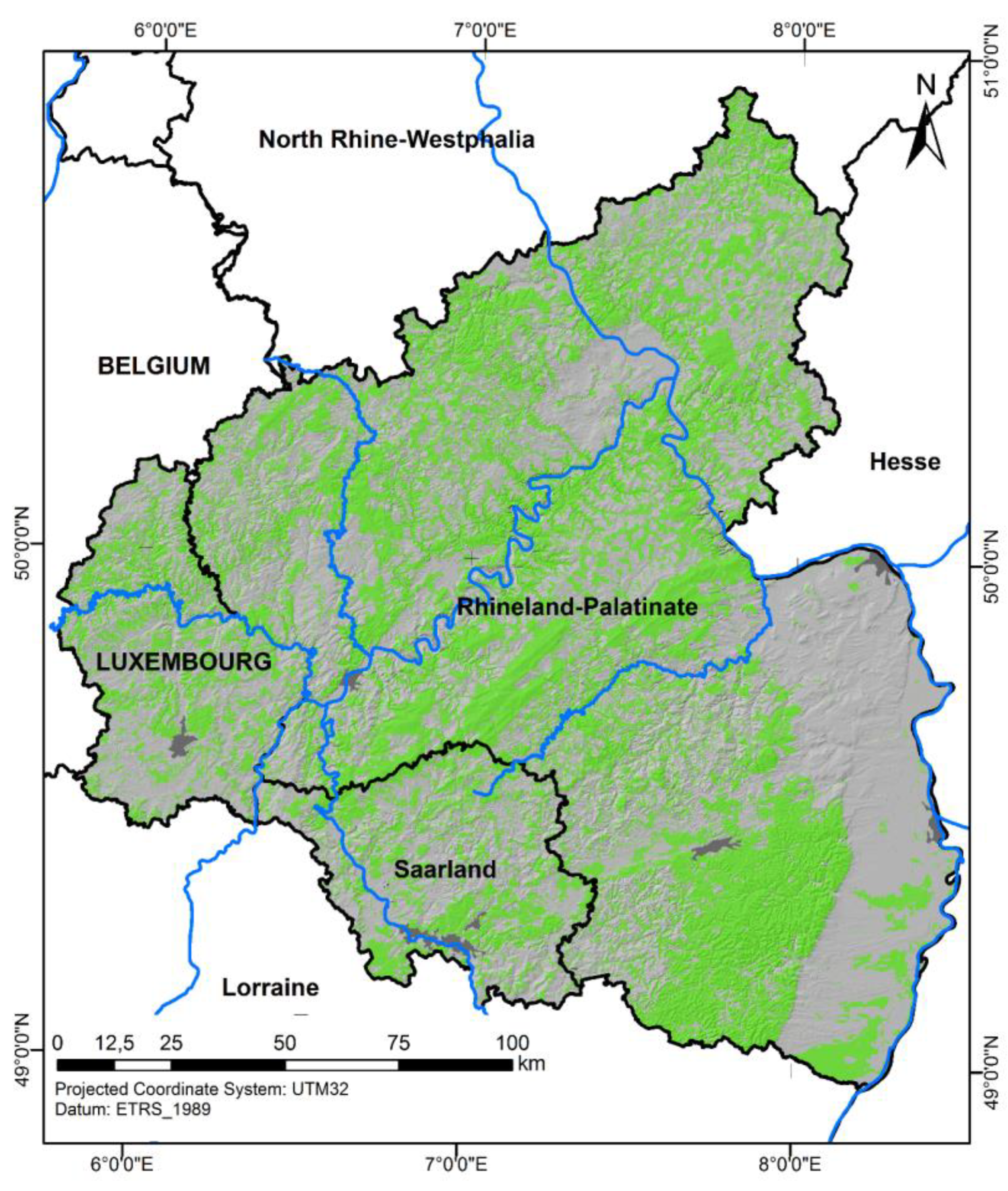
Funding

This work is part of Regiowood II, an EU-funded environmental project addressing forest monitoring in the Greater Region with the grant number 019-2-03-032. The authors gratefully acknowledge financial support through the INTERREG VA program in the Greater Region.

Acknowledgments

The authors are grateful for granting access to forest inventory data to the state forest service of Rhineland-Palatinate (Landesforsten Rheinland-Pfalz) and the Ministry of the Environment and Forestry of Rhineland-Palatinate (Ministerium für Umwelt, Forsten und Verbraucherschutz), to the state forest service of the Saarland (SaarForst Landesbetrieb) and to the state forest service of Luxembourg (Administration de la nature et des forêts). We also gratefully acknowledge the very helpful comments of all anonymous reviewers who helped to substantially improve the manuscript.

Conflicts of Interest

The authors declare no conflict of interest.

References

  1. Bellassen, V.; Luyssaert, S. Carbon sequestration: Managing forests in uncertain times. Nature 2014, 506, 153–155. [Google Scholar] [CrossRef] [PubMed] [Green Version]
  2. Potapov, P.V.; Yaroshenko, A.; Turubanova, S.; Dubinin, M.; Laestadius, L.; Thies, C.; Aksenov, D.; Egorov, A.; Yesipova, Y.; Glushkov, I.; et al. Mapping the World’s Intact Forest Landscapes by Remote Sensing. Ecol. Soc. 2008, 13, 51. [Google Scholar] [CrossRef]
  3. FAO. Global Forest Resources Assessment 2010; Main Report; Food and Agriculture Organization of the United Nations: Rome, Italy, 2010; ISBN 9789251066546. [Google Scholar]
  4. Hansen, M.C.; Potapov, P.V.; Moore, R.; Hancher, M.; Turubanova, S.A.; Tyukavina, A.; Thau, D.; Stehman, S.V.; Goetz, S.J.; Loveland, T.R.; et al. High-resolution global maps of 21st-century forest cover change. Science 2013, 342, 850–853. [Google Scholar] [CrossRef] [PubMed]
  5. Ministerium der Justiz Rheinland-Pfalz. Landeswaldgesetz. LWaldG; Ministerium der Justiz Rheinland-Pfalz: Mainz, Germany, 2000.
  6. Gesetz zur Erhaltung des Waldes und zur Förderung der Forstwirtschaft (Bundeswaldgesetz). BWaldG; BGBl. I S.: Berlin, Germany, 2017.
  7. United Nations Framework Convention on Climate Change. The Kyoto Protocol to the Convention on Climate Change. 1998. Available online: https://unfccc.int/resource/docs/convkp/kpeng.pdf (accessed on 3 October 2019).
  8. Humphreys, D. Negotiating the future under the shadow of the past: The eleventh session of the United Nations Forum on Forests and the 2015 renewal of the international arrangement on forests. Int. For. Rev. 2015, 17, 385–399. [Google Scholar] [CrossRef]
  9. Suding, K.; Higgs, E.; Palmer, M.; Callicott, J.B.; Anderson, C.B.; Baker, M.; Gutrich, J.J.; Hondula, K.L.; LaFevor, M.C.; Larson, B.M.H.; et al. Conservation. Committing to ecological restoration. Science 2015, 348, 638–640. [Google Scholar] [CrossRef] [PubMed]
  10. Forest Europe. Oslo Ministerial Decision: European Forests 2020. 2011. Available online: https://www.foresteurope.org/docs/MC/MC_oslo_decision.pdf (accessed on 20 November 2018).
  11. Kempeneers, P.; Sedano, F.; Seebach, L.; Strobl, P.; San-Miguel-Ayanz, J. Data Fusion of Different Spatial Resolution Remote Sensing Images Applied to Forest-Type Mapping. IEEE Trans. Geosci. Remote Sens. 2011, 49, 4977–4986. [Google Scholar] [CrossRef]
  12. Langanke, T. Copernicus Land Monitoring Service—High Resolution Layer Forest: Product Specifications Document; European Environmental Agency: Copenhagen, Denmark, 2017.
  13. Reese, H.; Nilsson, M.; Granqvist Pahlén, T.; Hagner, O.; Tingelöf, U.; Egberth, M.; Olsson, H. Countrywide Estimates of Forest Variables Using Satellite Data and Field Data from the National Forest Inventory. AMBIO 2003, 32, 542–548. [Google Scholar] [CrossRef] [PubMed]
  14. McInerney, D.O.; Nieuwenhuis, M. A comparative analysis of k NN and decision tree methods for the Irish National Forest Inventory. Int. J. Remote Sens. 2009, 30, 4937–4955. [Google Scholar] [CrossRef]
  15. Tomppo, E.; Katila, M.; Mäkisara, K.; Peräsaari, J. The Multi-source National Forest Inventory of Finland—Methods and results 2007. In Working Papers of the Finnish Forest Research Institute; Finnish Forest Research Institute: Vantaa, Finland, 2012. [Google Scholar]
  16. McRoberts, R.; Tomppo, E. Remote sensing support for national forest inventories. Remote Sens. Environ. 2007, 110, 412–419. [Google Scholar] [CrossRef]
  17. Næsset, E.; Gobakken, T.; Solberg, S.; Gregoire, T.G.; Nelson, R.; Ståhl, G.; Weydahl, D. Model-assisted regional forest biomass estimation using LiDAR and InSAR as auxiliary data: A case study from a boreal forest area. Remote Sens. Environ. 2011, 115, 3599–3614. [Google Scholar] [CrossRef]
  18. Nilsson, M.; Bohlin, J.; Olsson, H.; Svensson, S.A.; Haapaniemi, M. Operational use of remote sensing for regional level assessment of forest estate values. In New Strategies for European Remote Sensing: Proceedings of the 24th Symposium of the European Association of Remote Sensing Laboratories, Dubrovnik, Croatia, 25–27 May 2004; Oluić, M., Ed.; Millpress: Rotterdam, The Netherlands, 2005; pp. 263–268. ISBN 905966003X. [Google Scholar]
  19. Potapov, P.; Turubanova, S.; Hansen, M.C. Regional-scale boreal forest cover and change mapping using Landsat data composites for European Russia. Remote Sens. Environ. 2011, 115, 548–561. [Google Scholar] [CrossRef]
  20. Stoffels, J.; Hill, J.; Sachtleber, T.; Mader, S.; Buddenbaum, H.; Stern, O.; Langshausen, J.; Dietz, J.; Ontrup, G. Satellite-Based Derivation of High-Resolution Forest Information Layers for Operational Forest Management. Forests 2015, 6, 1982–2013. [Google Scholar] [CrossRef]
  21. Dees, M.; Duvenhorst, J.; Gross, C.P.; Koch, B. Combining Remote Sensing Data Sources and Terrestrial Sample-Based Inventory Data for the Use In Forest Management Inventories. In International Archives of Photogrammetry and Remote Sensing; Beek, K.J., Molenaar, M., Eds.; GITC BV: Amsterdam, The Netherlands, 2000; pp. 355–362. [Google Scholar]
  22. Diemer, C.; Lucaschewsky, I.; Spelsberg, G.; Tomppo, E.; Pekkarinen, A. Integration of terrestrial forest sample plot data, map information and satellite data: An operational multisource inventory concept. In Fusion of Earth Data: Merging Point Measurements, Raster Maps and Remotely Sensed Images, Proceedings of the Fusion of Earth Data, The Third International Conference, Sophia Antipolis, Côte d’Azur, France, 26–28 January 2000; Ranchin, T., Wald, L., Eds.; SEE/URISCA: Nice, France, 2000; pp. 143–150. [Google Scholar]
  23. Magnussen, S.; Boudewyn, P.; Wulder, M. Contextual classification of Landsat TM images to forest inventory cover types. Int. J. Remote Sens. 2004, 25, 2421–2440. [Google Scholar] [CrossRef]
  24. Buddenbaum, H.; Schlerf, M.; Hill, J. Classification of coniferous tree species and age classes using hyperspectral data and geostatistical methods. Int. J. Remote Sens. 2005, 26, 5453–5465. [Google Scholar] [CrossRef]
  25. Dorren, L.K.A.; Maier, B.; Seijmonsbergen, A.C. Improved Landsat-based forest mapping in steep mountainous terrain using object-based classification. For. Ecol. Manag. 2003, 183, 31–46. [Google Scholar] [CrossRef]
  26. Hagner, O.; Reese, H. A method for calibrated maximum likelihood classification of forest types. Remote Sens. Environ. 2007, 110, 438–444. [Google Scholar] [CrossRef]
  27. Ruefenacht, B.; Finco, M.V.; Nelson, M.D.; Czaplewski, R.; Helmer, E.H.; Blackard, J.A.; Holden, G.R.; Lister, A.J.; Salajanu, D.; Weyermann, D.; et al. Conterminous U.S. and Alaska Forest Type Mapping Using Forest Inventory and Analysis Data. Photogramm. Eng. Remote Sens. 2008, 74, 1379–1388. [Google Scholar] [CrossRef] [Green Version]
  28. Li, M.; Im, J.; Beier, C. Machine learning approaches for forest classification and change analysis using multi-temporal Landsat TM images over Huntington Wildlife Forest. Gisci. Remote Sens. 2013, 50, 361–384. [Google Scholar] [CrossRef]
  29. Gagliano, C.; De Natale, F.; Incerti, F.; Maselli, F. Alternative application of the k-NN Method for mapping forest cover type. In Proceedings of the ISPRS Working Group VII/1 Workshop ISPMSRS’07, Physical Measurements and Signatures in Remote Sensing, Davos, Switzerland, 12–14 March 2007; Schaepman, M.E., Liang, S., Groot, N., Kneubühler, M., Eds.; ISPRS: Davos, Switzerland, 2007. [Google Scholar]
  30. Tomppo, E.O.; Gagliano, C.; De Natale, F.; Katila, M.; McRoberts, R.E. Predicting categorical forest variables using an improved k-Nearest Neighbour estimator and Landsat imagery. Remote Sens. Environ. 2009, 113, 500–517. [Google Scholar] [CrossRef]
  31. Jinguo, Y.; Wei, W. Identification of Forest Vegetation Using Vegetation Indices. Chin. J. Popul. Resour. Environ. 2004, 2, 12–16. [Google Scholar] [CrossRef]
  32. Tao, H.; Li, M.; Wang, M.; Lü, G. Genetic algorithm-based method for forest type classification using multi-temporal NDVI from Landsat TM imagery. Ann. GIS 2019, 25, 33–43. [Google Scholar] [CrossRef]
  33. Erhard, M.; Wolff, B. Waldökologische Naturräume Deutschlands: Forstliche Wuchsgebiete und Wuchsbezirke. Klima. In Waldökologische Naturräume Deutschlands: Forstliche Wuchsgebiete und Wuchsbezirke; mit Karte 1:1.000.000; Gauer, J., Aldinger, E., Eds.; Verein für Forstliche Standortskunde und Forstpflanzenzüchtung: Freiburg, Germany, 2005; pp. 25–29. [Google Scholar]
  34. Landesforsten Rheinland-Pfalz. Landeswaldinventur: Emmelshausen, Germany. 2012. Available online: http://www.lebensenergie-riegelsberg.de/downloads/WBRL_Nov_2008aktuell.pdf (accessed on 3 October 2019).
  35. Ministerium für Umwelt und Verbraucherschutz Saarland. Forsteinrichtung; SaarForst Landesbetrieb: Saarbrücken, Germany, 2010.
  36. Administration de la Nature et des Forêts. Administrative Units of Forest Administration. Available online: https://data.public.lu/en/datasets/administrative-units-of-forest-administration/ (accessed on 20 March 2019).
  37. Landesforsten Rheinland-Pfalz. wöFIS: Waldökologisches Forstinformationssystem. Emmelshausen. 2016. Available online: https://www.kastanien.net/de/data/_uploaded/pdf/40projekte/aktuell_74-15_edelkastanie_am_oberrhein.pdf (accessed on 3 October 2019).
  38. Peerenboom, H.G.; Ontrup, G.; Böhmer, O. Weiterentwicklung der Forsteinrichtung in Rheinland-Pfalz. For. Und Holz 2003, 58, 728–731. [Google Scholar]
  39. Administration de la Nature et des Forêts. La Planification de la Gestion des Forêts Publiques. Available online: https://environnement.public.lu/fr/natur/forets/gestion_durable_forets_publiques.html (accessed on 13 March 2019).
  40. Ministerium für Umwelt und Verbraucherschutz Saarland. SaarForst Landesbetrieb; Privatwaldinventur: Saarbrücken, Germany, 2014.
  41. Riedel, T.; Hennig, P.; Kroiher, F.; Polley, H.; Schmitz, F.; Schwitzgebel, F. Die dritte Bundeswaldinventur (BWI 2012). Inventur- und Auswertungsmethoden; Bundesministerium für Ernährung und Landwirtschaft (BMEL): Berlin, Germany, 2017.
  42. Rondeux, J.; Wagner, M.; Kugener, G.; Saidi, M. L’inventaire forestier national permanent du Grand-Duché de Luxembourg, dix années d’existence. Wallone 2009, 103, 3–16. [Google Scholar]
  43. Administration de la Nature et Des Forêts; Inventure National des Forêts Luxembourg: Luxembourg, 2010.
  44. Chen, J.M.; Cihlar, J. Retrieving leaf area index of boreal conifer forests using Landsat TM images. Remote Sens. Environ. 1996, 55, 153–162. [Google Scholar] [CrossRef]
  45. Loveland, T.R.; Irons, J.R. Landsat 8: The plans, the reality, and the legacy. Remote Sens. Environ. 2016, 185, 1–6. [Google Scholar] [CrossRef] [Green Version]
  46. Drusch, M.; Del Bello, U.; Carlier, S.; Colin, O.; Fernandez, V.; Gascon, F.; Hoersch, B.; Isola, C.; Laberinti, P.; Martimort, P.; et al. Sentinel-2: ESA’s Optical High-Resolution Mission for GMES Operational Services. Remote Sens. Environ. 2012, 120, 25–36. [Google Scholar] [CrossRef]
  47. Fletcher, K. (Ed.) ESA’s Optical High-Resolution Mission for GMES Operational Services; ESA Communications: Noordwijk, The Netherlands, 2012; ISBN 978-92-9221-419-7. [Google Scholar]
  48. Woodcock, C.E.; Allen, R.; Anderson, M.; Belward, A.; Bindschadler, R.; Cohen, W.; Gao, F.; Goward, S.N.; Helder, D.; Helmer, E.; et al. Free access to Landsat imagery. Science 2008, 320, 1011. [Google Scholar] [CrossRef] [PubMed]
  49. Frantz, D. FORCE—Landsat + Sentinel-2 Analysis Ready Data and Beyond. Remote Sens. 2019, 11, 1124. [Google Scholar] [CrossRef]
  50. Kaufman, Y.J.; Tanre, D. Atmospherically resistant vegetation index (ARVI) for EOS-MODIS. IEEE Trans. Geosci. Remote Sens. 1992, 30, 261–270. [Google Scholar] [CrossRef]
  51. Frantz, D.; Röder, A.; Stellmes, M.; Hill, J. An Operational Radiometric Landsat Preprocessing Framework for Large-Area Time Series Applications. IEEE Trans. Geosci. Remote Sens. 2016, 54, 3928–3943. [Google Scholar] [CrossRef]
  52. Tanré, D. Description of a computer code to simulate signal in the solar spectrum: The 5S code. Int. J. Remote Sens. 1990, 11, 659–668. [Google Scholar] [CrossRef]
  53. Frantz, D.; Haß, E.; Uhl, A.; Stoffels, J.; Hill, J. Improvement of the Fmask algorithm for Sentinel-2 images: Separating clouds from bright surfaces based on parallax effects. Remote Sens. Environ. 2018, 215, 471–481. [Google Scholar] [CrossRef]
  54. Tucker, C.J. Red and photographic infrared linear combinations for monitoring vegetation. Remote Sens. Environ. 1979, 8, 127–150. [Google Scholar] [CrossRef] [Green Version]
  55. Gascon, F.; Bouzinac, C.; Thépaut, O.; Jung, M.; Francesconi, B.; Louis, J.; Lonjou, V.; Lafrance, B.; Massera, S.; Gaudel-Vacaresse, A.; et al. Copernicus Sentinel-2A Calibration and Products Validation Status. Remote Sens. 2017, 9, 584. [Google Scholar] [CrossRef]
  56. Xue, J.; Su, B. Significant Remote Sensing Vegetation Indices: A Review of Developments and Applications. J. Sens. 2017, 2017, 1353691. [Google Scholar] [CrossRef]
  57. Huete, A. A comparison of vegetation indices over a global set of TM images for EOS-MODIS. Remote Sens. Environ. 1997, 59, 440–451. [Google Scholar] [CrossRef]
  58. Pearson, R.L. Remote mapping of standing crop biomass for estimation of the productivity of the short-grass Prairie. In Proceedings of the International Sympathy on Remote Sensing of Environment, Ann Arbor, MI, USA, 2–6 October 1972. [Google Scholar]
  59. Rouse, J.W. Monitoring the Vernal Advancement and Retrogradation of Natural Vegetation; NASA/GSFCT Type II Report; NASA: Greenbelt, MD, USA, 1973.
  60. Huete, A.R. A soil-adjusted vegetation index (SAVI). Remote Sens. Environ. 1988, 25, 295–309. [Google Scholar] [CrossRef]
  61. Roujean, J.-L.; Breon, F.-M. Estimating PAR absorbed by vegetation from bidirectional reflectance measurements. Remote Sens. Environ. 1995, 51, 375–384. [Google Scholar] [CrossRef]
  62. Crippen, R. Calculating the vegetation index faster. Remote Sens. Environ. 1990, 34, 71–73. [Google Scholar] [CrossRef]
  63. Huete, A.; Didan, K.; Miura, T.; Rodriguez, E.P.; Gao, X.; Ferreira, L.G. Overview of the radiometric and biophysical performance of the MODIS vegetation indices. Remote Sens. Environ. 2002, 83, 195–213. [Google Scholar] [CrossRef]
  64. Efron, B. Bootstrap Methods: Another Look at the Jackknife. Ann. Stat. 1979, 7, 1–26. [Google Scholar] [CrossRef]
  65. Olofsson, P.; Foody, G.M.; Herold, M.; Stehman, S.V.; Woodcock, C.E.; Wulder, M.A. Good practices for estimating area and assessing accuracy of land change. Remote Sens. Environ. 2014, 148, 42–57. [Google Scholar] [CrossRef]
  66. Congalton, R.G. A review of assessing the accuracy of classifications of remotely sensed data. Remote Sens. Environ. 1991, 37, 35–46. [Google Scholar] [CrossRef]
  67. Schönthaler, K. (Ed.) Monitoringbericht 2015 zur Deutschen Anpassungsstrategie an den Klimawandel. Bericht der Interministeriellen Arbeitsgruppe Anpassungsstrategie der Bundesregierung; Umweltbundesamt: Dessau-Roßlau, Germany, 2015.
  68. Nink, S.; Hill, J.; Buddenbaum, H.; Stoffels, J.; Sachtleber, T.; Langshausen, J. Assessing the Suitability of Future Multi- and Hyperspectral Satellite Systems for Mapping the Spatial Distribution of Norway Spruce Timber Volume. Remote Sens. 2015, 7, 12009–12040. [Google Scholar] [CrossRef] [Green Version]
Figure 1. Map of the study area. Forest areas based on cadastral data are depicted in light green.
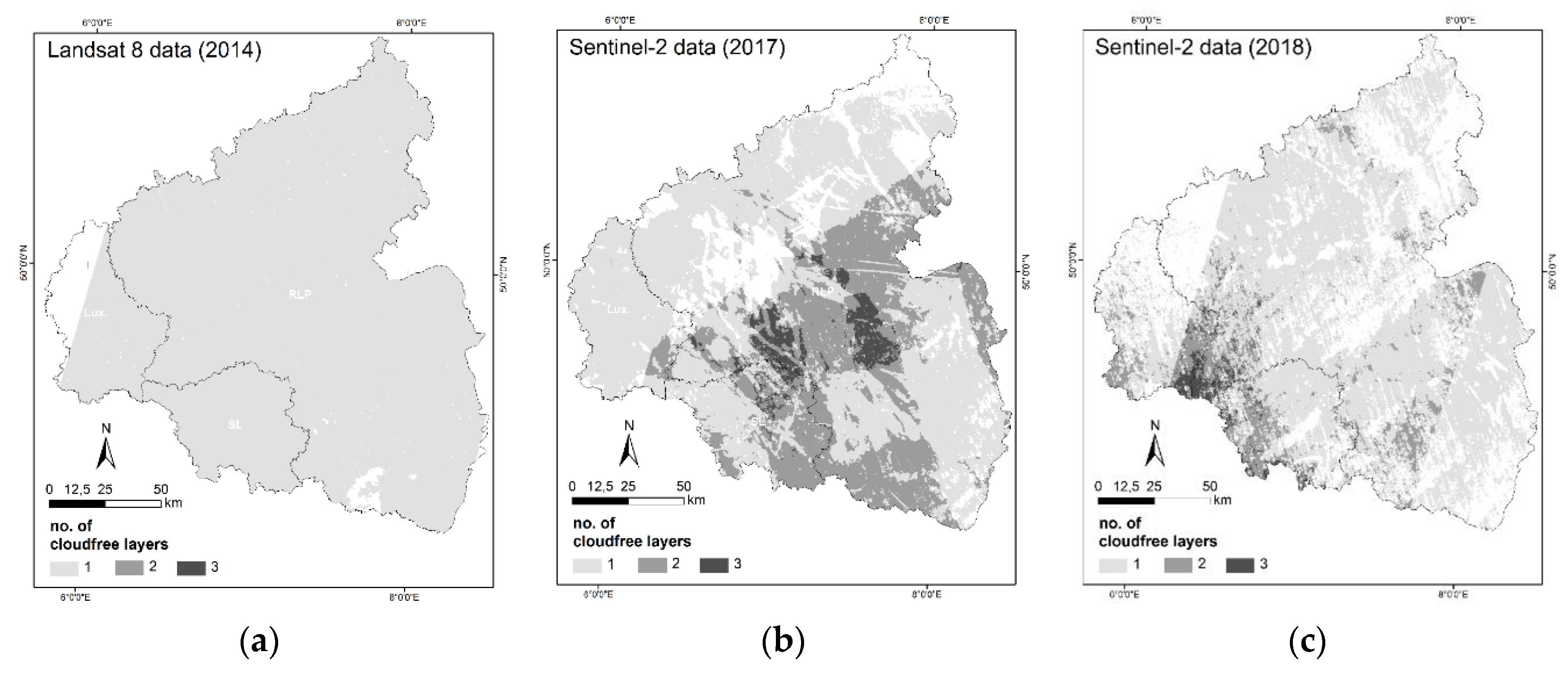
Remotesensing 11 02337 g001
Figure 2. Coverage of satellite data in 2014 (a), 2017 (b) and 2018 (c). White areas represent no data, light grey areas one, grey areas two and dark grey areas three image acquisitions in the respective year.
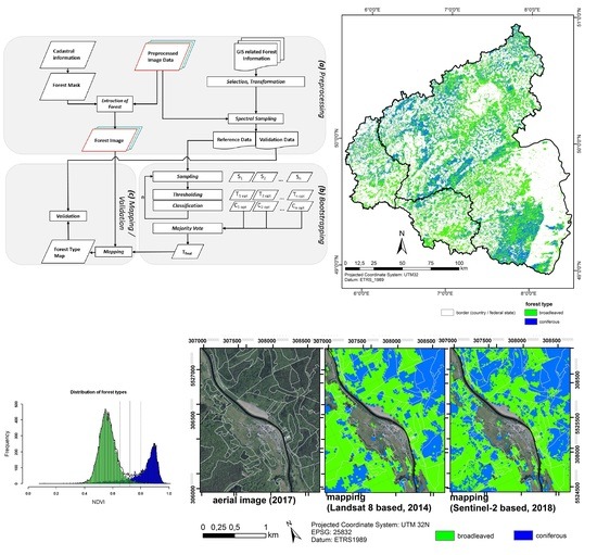
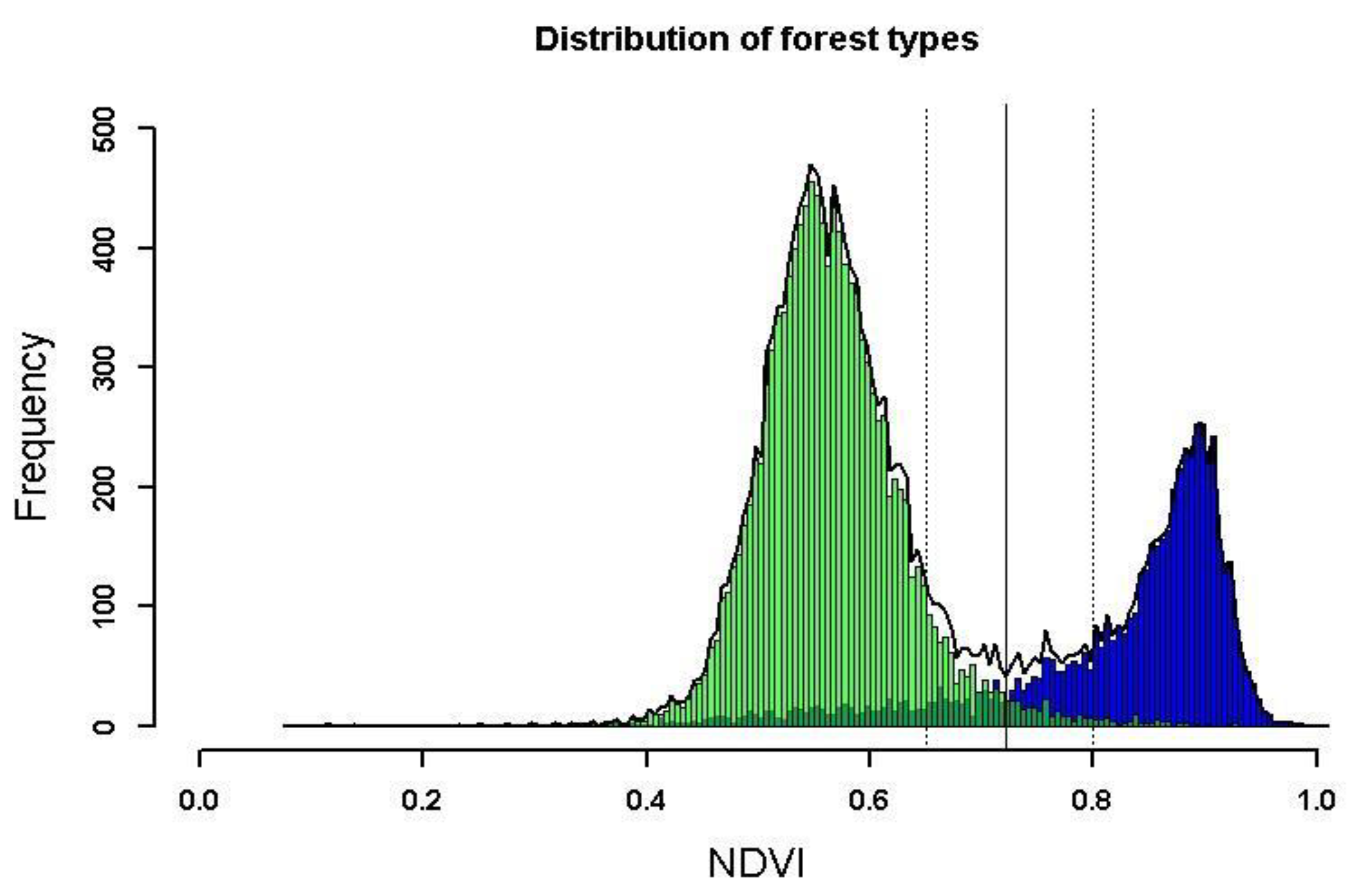
Remotesensing 11 02337 g002
Figure 3. Distribution of broadleaved (green) and coniferous (blue) tree species in the reference data extracted from the Landsat 8 image. The black line depicts the sum of both classes. The vertical black line indicates the minimum turning point, the vertical dotted lines the distance of one-half standard deviation in the dataset, which is used as range for threshold parameterization.
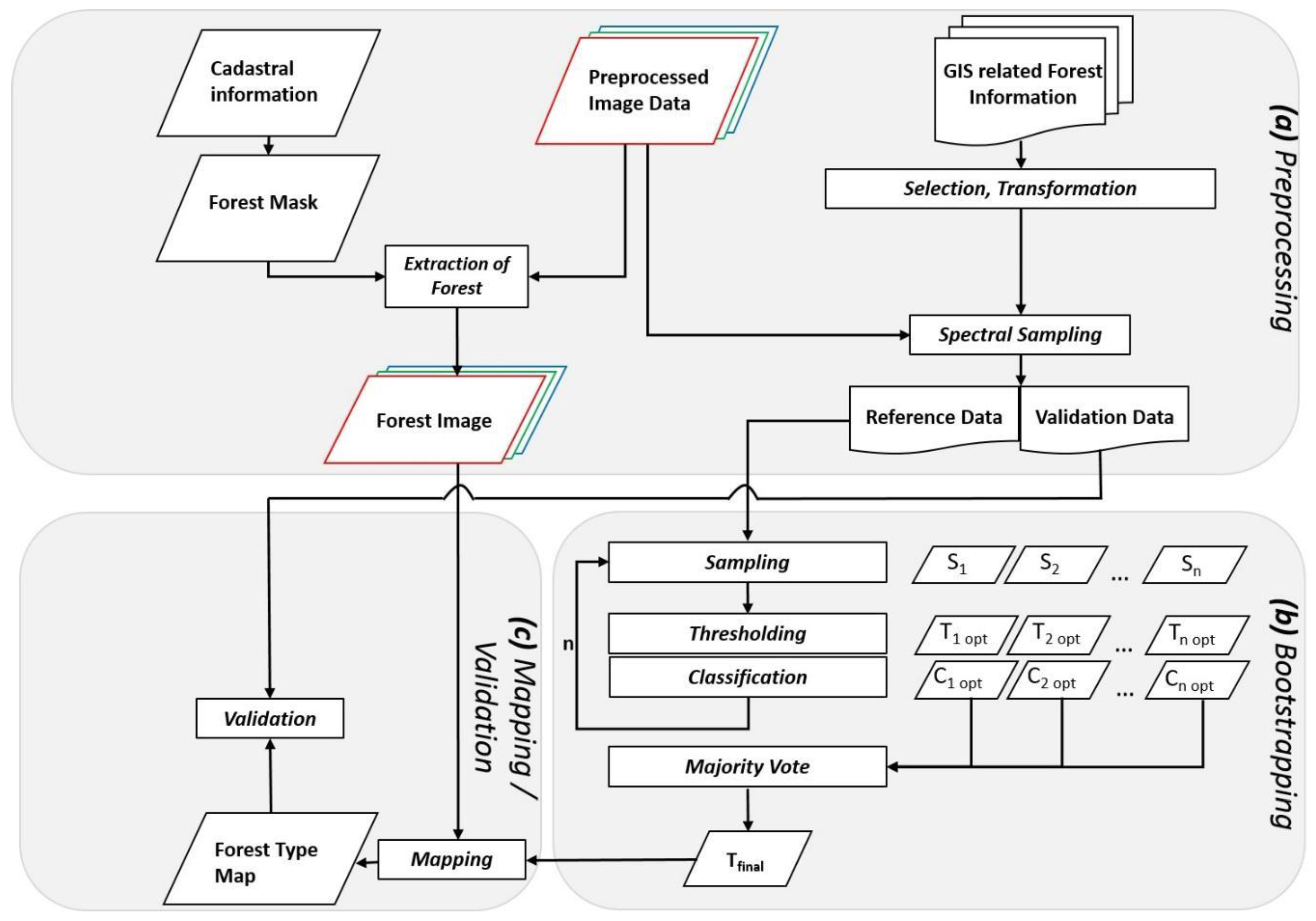
Remotesensing 11 02337 g003
Figure 4. Processing flowchart including the pre-processing part (a), the parameterization part based on the bootstrapping method (b) and the mapping and validation part (c).
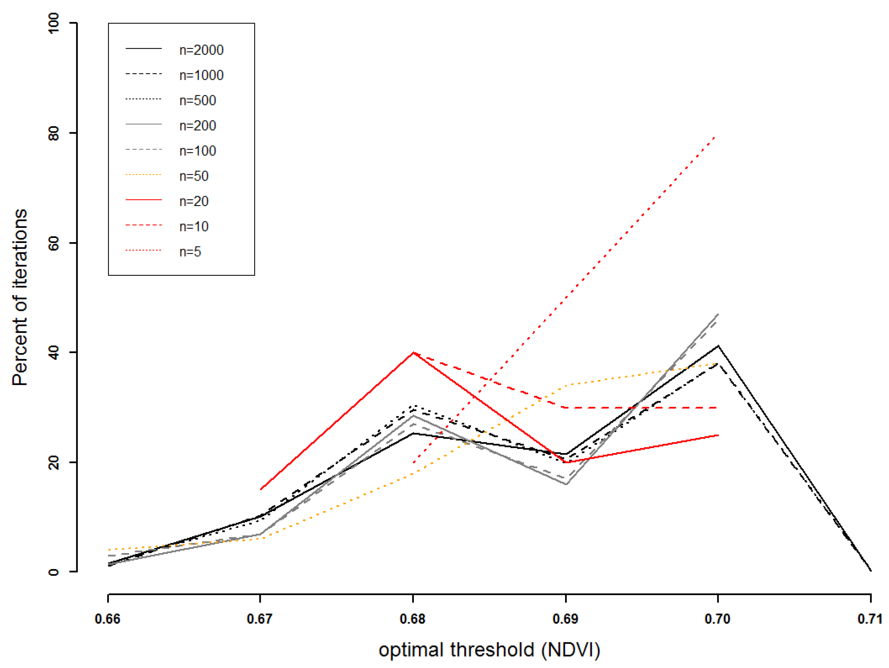
Remotesensing 11 02337 g004
Figure 5. The approximation of the optimal threshold for the separation of forest types is depending on the number of iterations. A stabilization occurs for more than 100 iterations.
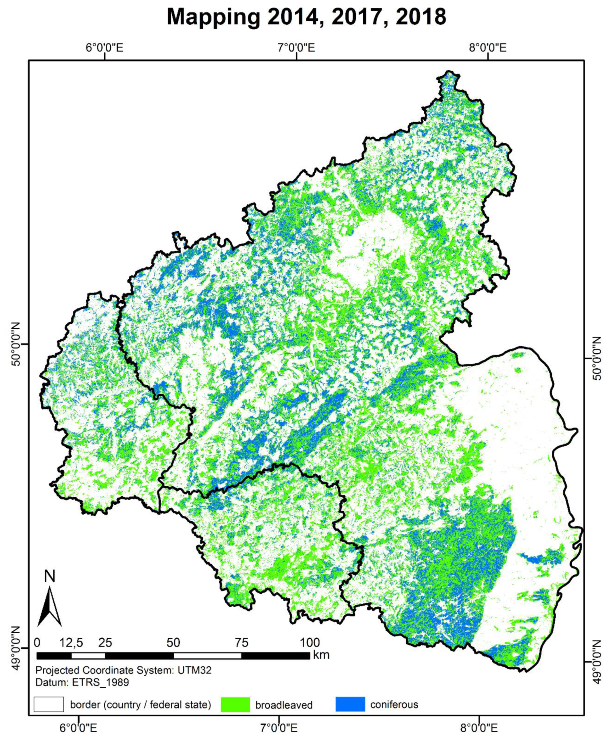
Remotesensing 11 02337 g005
Figure 6. Forest Type map based on Landsat 8 data from 2014, updated with Sentinel-2 imagery from 2017 and 2018.
Remotesensing 11 02337 g006
Figure 7. Depiction of the spatially explicit and consistent transnational forest type mapping in the border region Luxembourg/RLP and comparison of the mapping based on Landsat-8 and Sentinel-2 imagery.
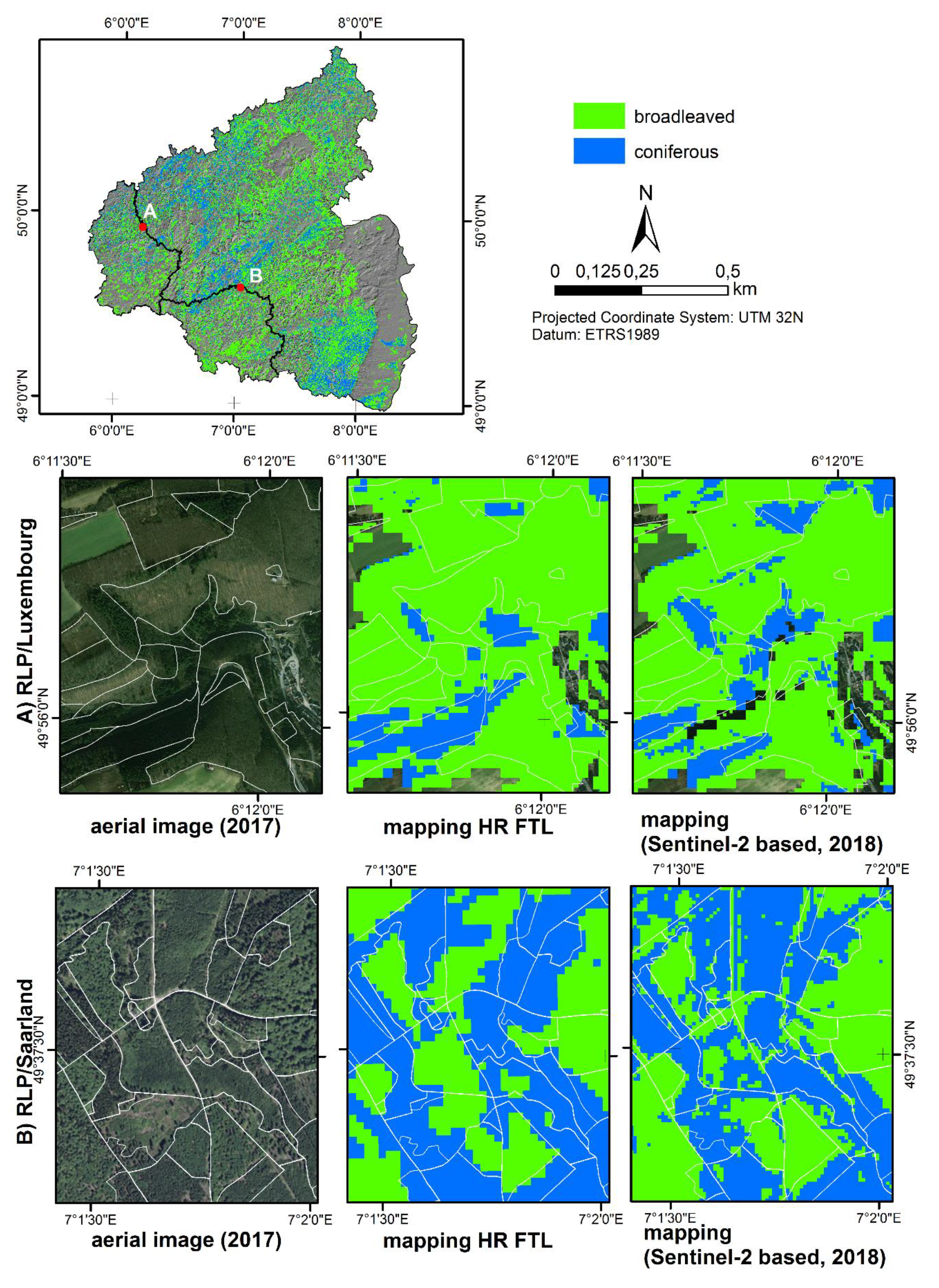
Remotesensing 11 02337 g007
Figure 8. Mapping of the Copernicus HR-FTL and the Sentinel-2 based prediction map in the border region of Luxembourg and RLP and the border region of RLP and the Saarland.
Remotesensing 11 02337 g008
Table 1. Overview of the forest cover and proportional forest cover considering the forest type.
Area [km2]Forest [km2]Forest [%]Broadleaved [%]Coniferous [%]
RLP19,847838842.2662.0337.97
Saarland257094636.8173.4926.51
Luxembourg258694036.2167.6432.36
Total250031027441.0763.3936.61
Table 2. Overview and characteristics of the available forest information systems.
NameCountry/Federal StateTypeNo. of ReferencesAcquisition Time
Forest Management Information (public forests)Rhineland-PalatinateArea-based150632003–2016
Federal State Forest InventoryRhineland-PalatinatePoint-based53342010
Forest Management Information (public forests)SaarlandArea-based12102010
Forest Management Information (private forests)SaarlandArea-based9112014
projected FSFI Grid 1SaarlandPoint-based3492010–2014
Forest Management InformationLuxembourgArea-based6972016
National Forest Inventory 2LuxembourgPoint-based3112010
1 information is related to official forest management information due to local unavailability of NFI/FSFI data. 2 The number of validation points from the NFI was reduced to be comparable to the spatial distribution in the other subregions.
Table 3. List of satellite images used in the study.
SensorDate of AcquisitionCloud Coverage [%]Forest in Footprint [ha]Forest Coverage in Footprint [%]
Landsat 82014-03-271.00996895.31
Sentinel-2A2017-03-1164.69570521.22
Sentinel-2A2017-03-1442.11777545.31
Sentinel-2A2017-04-204.32 169315.95 1
Sentinel-2B2018-03-1475.4437155.81
Sentinel-2B2018-03-2135.74906848.59
Sentinel-2B2018-03-2489.4252277.47
1 only areas higher than 500 m a.s.l. were used.
Table 4. Suitable Vegetation Indices and its most important properties used for the mapping of forest types.
NameEquationPropertiesReference
Simple Ratio S R = N I R / R Classic[58]
Difference VI D V I = N I R R Classic[54]
Normalized Difference VI N D V I = N I R R N I R + R Classic, normalized[59]
Renormalized Difference VI R D V I = N I R R / ( N I R + R ) 1 2 Adjusted, compensates sun view geometry[61]
Infrared Percentage VI I P V I = N I R N I R + R Simplified NDVI[62]
Soil Adjusted VI S A V I = ( N I R R ) N I R + R + L ( 1 + L ) Soil, background adjusted; L = 0.5[60]
Atmospherically Resistant VI A R V I = N I R ( R y ( B R ) ) N I R + ( R y ( B R ) ) Atmospheric effects adjusted;
y = 1
[50]
Soil and Atmospherically Resistant VI S A R V I = N I R ( R y ( B R ) ) N I R + ( R y ( B R ) ) + L ( 1 + L ) Combines adjustment of soil, background and atmospheric effects; L = 0.5[50]
Enhanced VI E V I = G ( N I R R ) ( N I R + C 1 × R C 2 × B + L ) background and atmospheric effects[63]
Table 5. Parameterization to receive the optimal threshold (area under the ROC curve) and comparison of the received OAA based on Landsat 8 and Sentinel-2 derived VIs.
IndexData RangeParameterizationValidation
AUCThresholdOAA
L8S-2L8S-2L8S-2
RLPSaarLuxRLPSaarLux
SR0–260.920.945.604.50.830.790.950.870.810.93
DVI142–32900.690.78136012800.640.650.640.740.730.77
NDVI0.08–10.920.930.700.640.830.790.960.870.820.93
RDVI4.98–51.50.870.8930.0028.20.780.750.790.840.810.87
IPVI0.27–10.920.940.430.820.830.740.960.870.820.91
SAVI0.12–1.510.930.921.040.960.830.780.940.870.820.92
ARVI0.04–1.110.910.940.610.580.830.780.940.870.820.93
SARVI−0.1–2.30.920.940.910.880.830.780.930.870.820.93
EVI−22–740.900.931.801.950.800.760.890.850.790.92
Table 6. Comparison of the mappings based on suitable Landsat 8 and Sentinel-2 VIs stratified by subregion. S(Area) reports the standard error for estimated area in hectares, S(OAA) for overall accuracy, S(UA) for the user’s and S(PA) for the producer’s accuracy; the subscript b stands for broadleaved and c for coniferous class.
Landsat 8 (2014)Sentinel-2 (2017/18)
MinMaxMinMax
S(Area) RLP1083183512481851
Saarland2341263316962088
Luxembourg4478569734104746
S(OAA)RLP0.01670.02840.01570.0233
Saarland0.02180.02450.03290.0242
Luxembourg0.00550.00690.0050.0069
S(UAb)RLP0.00930.02450.01180.0207
Saarland0.0230.02750.02080.0253
Luxembourg0.00690.00860.00660.0086
S(UAc)RLP0.05640.07970.04260.0529
Saarland0.04950.05730.05960.0656
Luxembourg0.00880.01160.00740.0113
S(PAb)RLP0.00860.01780.01110.0166
Saarland0.02010.02120.01820.0216
Luxembourg0.00620.00650.00620.0069
S(PAc)RLP0.04410.07800.03830.0459
Saarland0.03530.04060.04330.0481
Luxembourg0.00680.00820.00610.0083
Table 7. Error matrix of estimated proportions of area (bootstrap based prediction map using Sentinel-2 derived NDVI in RLP).
Validation Data
BroadleavedConiferousTotal (Wi)Area [ha]
MapBroadleaved0.53870.09320.6320563,158
Coniferous0.04350.32450.3680328,023
Total0.58230.41771891,182
Area [ha]518,887372,295
Table 8. Error matrix of estimated proportions of area (bootstrap based prediction map using Sentinel-2 derived NDVI in the Saarland).
Validation Data
BroadleavedConiferousTotal (Wi)Area [ha]
MapBroadleaved0.68030.09150.771888,278
Coniferous0.08630.14190.228226,104
Total0.76650.23351114,382
Area [ha]87,67926,703
Table 9. Error matrix of estimated proportions of area (bootstrap based prediction map using Sentinel-2 derived NDVI in Luxembourg).
Validation Data
BroadleavedConiferousTotal (Wi)Area [ha]
MapBroadleaved0.65430.03900.693366,950
Coniferous0.04720.25950.306729,619
Total0.70150.2985196,569
Area [ha]67,73928,830
Table 10. Error matrices of estimated proportions of area for the HR-FTL in RLP.
Validation Data
BroadleavedConiferousTotal (Wi)Area [ha]
HR-
FTL
Broadleaved0.55220.09860.6509613,760
Coniferous0.05250.29660.3491329,252
Total0.60470.39531943,012
Area [ha]570,271372,741
Table 11. Error matrices of estimated proportions of area for the HR-FTL in the Saarland.
Validation Data
BroadleavedConiferousTotal (Wi)Area [ha]
HR-
FTL
Broadleaved0.64400.11760.761795,531
Coniferous0.07560.16280.238329,890
Total0.71960.28041125,420
Area [ha]90,25435,166
Table 12. Error matrices of estimated proportions of area for the HR-FTL in Luxembourg.
Validation Data
BroadleavedConiferousTotal (Wi)Area [ha]
HR-
FTL
Broadleaved0.70990.03550.745475,404
Coniferous0.03230.22230.254625,758
Total0.74220.25781101,162
Area [ha]75,08426,078
Table 13. Validation of the HR-FTL and the mapping approach (Updated map based on the NDVI) reporting the OAA, user’s (UA) and producer’s accuracy (PA) for mapped broadleaved (subscript b) and coniferous forest (subscript c) in the three subregions.
OAAUAbUAcPAbPAcWbWc
RLPFTL0.850.850.850.910.750.6510.349
Map0.860.850.880.930.780.6310.368
SaarFTL0.810.850.680.890.580.7620.238
Map0.820.880.620.890.610.7720.228
LuxFTL0.930.950.870.960.860.7450.255
Map0.920.950.850.930.880.6930.307
Table 14. Standard error for the mappings based on Landsat 8 and Sentinel-2 (NDVI) for each subregion. S(Area) reports the standard error for estimated area in hectares, S(OAA) for overall accuracy, S(UA) for the user’s and S(PA) for the producer’s accuracy; the subscript b stands for broadleaved, subscript c for coniferous class.
S(OAA) S(UAb)S(UAc)S(Area)
RLPFTL0.0050.00630.00824696
Map0.00480.00620.00744262
SaarFTL0.02110.02250.05172647
Map0.020.02040.05392283
LuxFTL0.01500.01400.04231519
Map0.01700.01470.04451644

