Kernel Entropy Component Analysis-Based Robust Hyperspectral Image Supervised Classification


1
School of Information Science and Technology, Hunan Institute of Science and Technology, Yueyang 414000, China
2
Guangxi Key Laboratory of Images and Graphics Intelligent Processing, Guilin University of Electronics Technology, Guilin 541000, China
*
Author to whom correspondence should be addressed.
†
Chengle Zhou is the co-first author.
Remote Sens. 2019, 11(23), 2823; https://0-doi-org.brum.beds.ac.uk/10.3390/rs11232823
Submission received: 30 October 2019
/
Revised: 20 November 2019
/
Accepted: 25 November 2019
/
Published: 28 November 2019
Abstract
:Recently, the “noisy label" problem has become a hot topic in supervised classification of hyperspectral images (HSI). Nonetheless, how to effectively remove noisy labels from a training set with mislabeled samples is a nontrivial task for a multitude of supervised classification methods in HSI processing. This paper is the first to propose a kernel entropy component analysis (KECA)-based method for noisy label detection that can remove noisy labels of a training set with mislabeled samples and improve performance of supervised classification in HSI, which consists of the following steps. First, the kernel matrix of training samples with noisy labels for each class can be achieved by exploiting a nonlinear mapping function to enlarge the sample separability. Then, the eigenvectors and eigenvalues of the kernel matrix can be obtained by employing symmetric matrix decomposition. Next, the entropy corresponding to each training sample in each class is calculated based on entropy component analysis using the eigenvalues arranged in descending order and the corresponding eigenvectors. Finally, the sigmoid function is applied to the entropy of each sample to obtain the probability distribution. Meanwhile, a decision probability threshold is introduced into the above probability distribution to cleanse the noisy labels of training samples with mislabeled samples for each class. The effectiveness of the proposed method is evaluated by support vector machines on several real hyperspectral data sets. The experimental results show that the proposed KECA method is more efficient than other noisy label detection methods in terms of improving performance of the supervised classification of HSI.
1. Introduction
Hyperspectral images (HSI) are captured by hundreds of continuous and narrow spectral bands while simultaneously reflecting interesting target areas. HSI offers the potential for the development of classification techniques because of the nature of different materials with different spectral information. Advancements in classification technology can bring high-level interpretations of remotely sensed scenes and are therefore now widely used in various application domains such as environmental monitoring [1,2], precision agriculture [3,4], and mineral exploration [5,6,7]. Specifically, these application scenarios are almost always highly dependent on supervised classification algorithms such as support vector machines (SVM) [8,9,10,11,12], sparse representation (SR) [13,14,15,16,17,18,19], naive Bayesian method [20,21,22], and decision trees [23,24,25]. In addition, most existing supervised classifiers are modeled based on the assumption that the labeled pixels used for training the classification model are highly trusted [26,27,28,29]. However, in practical applications, the acquisition of training samples usually generate mislabeled samples (noisy labels) that result in significant degradation of performance for the supervised classifier. Therefore, it is often necessary to denoise a training set with noisy labels, and then use the improved training set in subsequent experiments.
Unlike the “noisy” label issue in general computer vision applications, the appearance of noisy labels in hyperspectral remote sensing images can be summarized in three aspects: (1) Noisy labels caused by global position system (GPS) positioning errors. To obtain training samples, field exploration with GPS and the environment for visualizing images (ENVI) is the most convenient way to label pixels. However, the positioning accuracy of the GPS cannot satisfy by the spatial resolution of the pixel, and it is difficult to accurately distinguish the land cover distribution of candidate pixels. Once the GPS has a position error, land covers may be mislabeled, and thus may generate noisy labels. (2) Noisy labels caused by manual labeling errors. Labeling pixels with visual interpretation is the most reliable way of acquiring training samples. However, manual labeling requires a mass of manpower and a labeling expert who has knowledge of the environment that corresponds to the pixel to be labeled. Specifically, some noncongeneric land cover may exist for a large regular region. However, those noncongeneric regions are generally labeled as the same class as those of surrounding regions to reduce human effort. (3) Noisy labels caused by complex environmental factors. For some scenes, such as ocean and wetland, ground investigation is impossible since they may be unreachable for exploration experts. Moreover, labeling errors may also be produced due to other environmental factors such as adverse weather. In the above situations, the training sample acquisition process generally cannot avoid the generation of noisy labels. Therefore, we can conclude that the “noisy label” problem is, indeed, a major challenge in HSI classification.
For supervised classification in HSI, the noisy label problem of supervised task is increasingly becoming a focus of attention in the field of computer vision and remote sensing. For example, in computer vision, Xiao et al. [30] proposed a probabilistic graphical framework to train convolutional neural networks with a few clean labels and millions of noisy labels. Lu et al. [31] proposed an optimization-based sparse learning model to detect and remove noisy labels for semantic segmentation. Yao et al. [32] introduced a generative model called latent stability analysis to discover stable patterns among images with noisy labels. In remote sensing, Kang et al. [33] first introduced the reasons for the formation of noisy labels in HSI supervised classification and proposed an edge-preserving filtering (EPF) and spectral detection-based method to correct mislabeled training samples. Experiments show that this method can effectively remove noisy labels and improve the performance of supervised classifiers. Jiang et al. [34] proposed a random label propagation algorithm (RLPA) to cleanse the noisy labels in the training set, the key idea of RLPA is exploiting knowledge (e.g., the superpixel-based spectral-spatial constraints) from the observed hyperspectral images and applying it to the process of label propagation. The fusion spectral angle and local outlier factor (SALOF) are proposed to detect noisy labels in the HSI classification in [35]. Tu et al. [36,37] proposed a new density peak (DP) clustering-based noisy label detection method to detect noisy labels. The experimental results show that the DP-based detection method can effectively promote the classification performance. Jie et al. [38] provided a noisy label detection method based on joint spectral-spatial distributed sparse representation that exploits the intraband structure and the interband correlation in the process of joint sparse representation and joint dictionary learning.
In recent years, various processing technologies based on entropy analysis and the kernel method have been successfully applied in the HSI classification. For instance, He et al. [39] proposed an HSI anomaly detection algorithm based on maximum entropy and nonparametric estimation. According to the low probability of the target, the maximum entropy principle is used to estimate the probability density of the target, and the generalized likelihood ratio test is simplified to test only the background likelihood. Cheng et al. [40] proposed an image segmentation algorithm based on 2D Renyi gray entropy and fuzzy clustering. The traditional 2D Renyi threshold is replaced by a two-dimensional Renyi entropy thresholding to improve the global segmentation performance. The validating experiment shows the effectiveness of improved algorithm. Jie et al. [41] introduced a multiple kernel learning method based on discriminative kernel clustering (DKC) to choose the optimal bands in the HSI. The experiments were conducted on several real hyperspectral data sets to demonstrate that the effectiveness of the DKC band selection method in terms of classification performance and computation efficiency.
In this paper, a kernel entropy component analysis (KECA)-based noisy label detection method is proposed to improve training set with noisy labels in HSI supervised classification. The proposed method consists of the following steps: first, a kernel matrix of the training samples with noisy labels for each class can be created by exploiting the RBF kernel function. Then, the eigenvectors and eigenvalues of the kernel matrix can be obtained by employing symmetric matrix decomposition. Next, the entropy that corresponds to each training sample for each class is calculated based on entropy component analysis using the eigenvalues arranged in descending order and their corresponding eigenvectors. Finally, the sigmoid function is applied to the entropy of each sample to obtain the probability distribution. Meanwhile, a decision probability threshold is introduced into the above probability distribution to remove the noisy labels of the training set with mislabeled samples for each class. The major contributions of the proposed KECA method are presented as follows:
- KECA is first introduced into HSI supervised classification to cleanse the original training set with noisy labels. Noisy labels often have very high local entropies, which is the basic motivation behind this paper.
- Five commonly used kernel functions are analyzed in the proposed detection framework, where the RBF kernel function is found to be a robust kernel trick for detecting noisy labels.
- The effectiveness of proposed method is proved by adopting several real hyperspectral datasets and multiple classifiers, i.e., spectral classifiers and spectral-spatial classifiers. The experimental results show that the proposed KECA is more efficient than other noisy label detection methods in terms of improving performance of the supervised classification in HSI.
The rest of this paper is organized as follows. Entropy component analysis and related works are reviewed in Section 2. Section 3 describes the proposed KECA-based noise label detection method in detail. Section 4 analyzes the experimental results, Section 5 presents the extended discussion, and conclusions are given in Section 6.
2. Review of Related Methods
In this section, we briefly review the kernel tricks and the Renyi entropy method.
2.1. Kernel Tricks
Recently, some kernel tricks have been demonstrated that can provide optimal performance for HSI classification. For instance, Toksöz et al. [42] proposed a nonlinear kernel version of a recently introduced basic thresholding classifier for HSI classification that shows that the proposal and its spatial extension yield better classification results. Li et al. [43] presented a new framework for the development of generalized composite kernel machines for hyperspectral image classification that proved that the proposed framework could lead to state-of-the-art classification performance in complex analysis scenarios. Fang et al. [44] presented a novel framework to effectively utilize the spectral-spatial information of superpixels via multiple kernels that indicated that the proposed approach outperforms several well-known classification methods. Assume that and are pixels that belong to a sample set , where n represents the number of pixels. Then, the kernel function is expressed as follows:
where is a mapping function that maps a spectral vector from low-dimensional to high-dimensional. Furthermore, this section reviews several common kernel functions, radial basis function (RBF), linear kernel function (LKF), polynomial kernel function (PKF), wavelet kernel function (WKF), and Laplacian kernel function (LNKF).
- Radial basis function:where refers to the weight of the Gaussian function.
- Linear kernel function:where c refers to the constant term.
- Polynomial kernel function:where refers to the free parameter, and q is power term that controls the polynomial.
- Wavlet kernel function:where and are the mother wavelet function and the translation coefficients, respectively.
- Laplacian kernel function:
2.2. Renyi entropy
Suppose that is a probability density function on the sample set , the Renyi entropy can be defined as follows:
Then, the Parzen window density estimator is introduced by:
where is a Parzen window, which is also called the kernel density.
Finally, the entropy based on the Renyi method can be obtained as follows:
3. Proposed KECA Method for HSI Classification with Noisy Labels
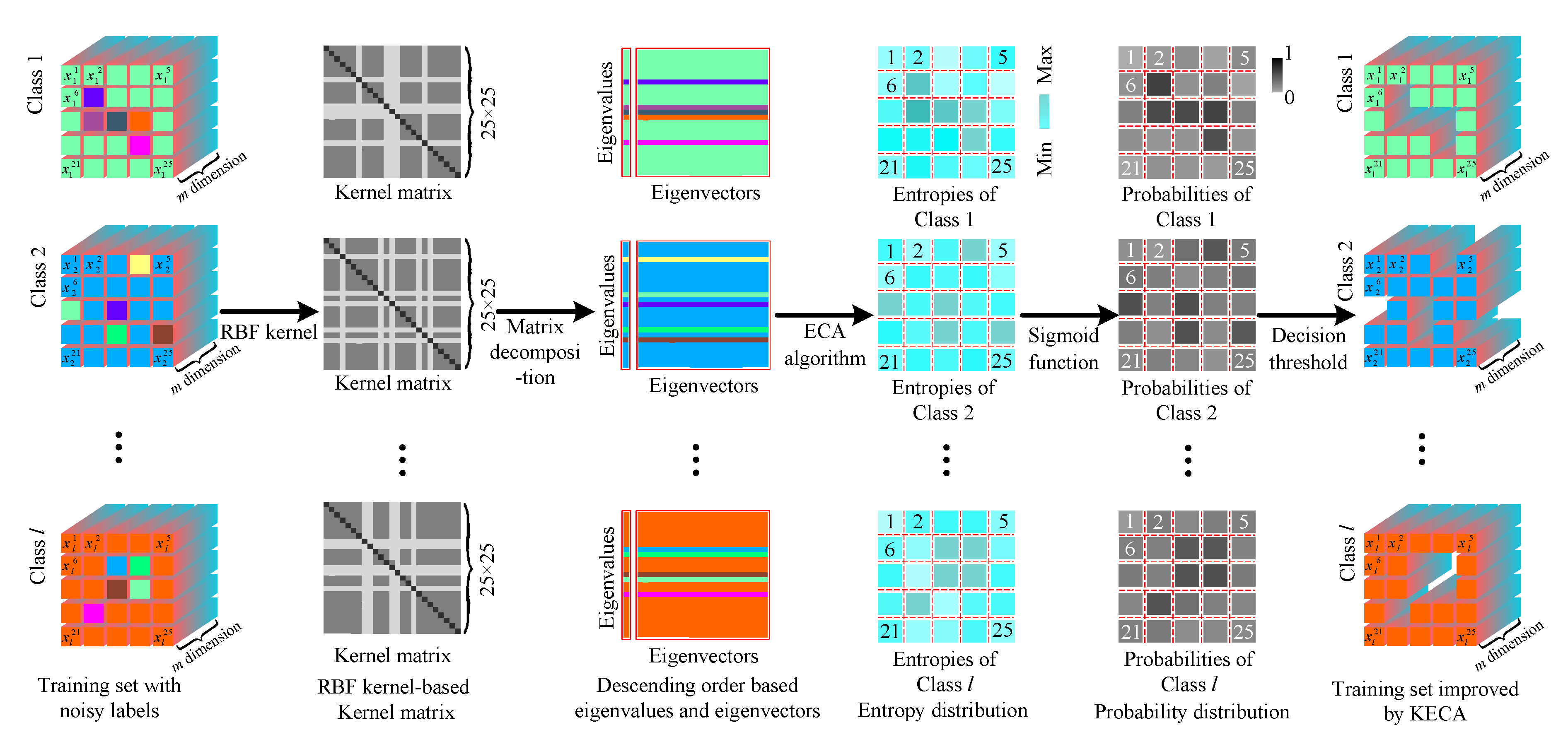
Unlike kernel principal component analysis (KPCA), KECA extracts low-dimensional features by considering both the magnitude of eigenvalues and the size of eigenvectors, which can achieve discriminative features from training samples of each class and better reflect the cluster structure. The KPCA only considers the ranking of the eigenvalues, and thus the latent discriminative feature of the training samples may be lost. This paper proposes a new noisy label detection method that extracts the features with the greatest contribution to the Renyi entropy, which is composed of the following parts: (1) Construct the kernel matrix; (2) Acquire the entropy distribution; and (3) Cleanse the training set with noisy labels. The proposed KECA method for noisy label detection is summarized as Algorithm 1 (see Figure 1). Each part consists of certain steps, the details of which are presented as follows.
| Algorithm 1. KECA. |
| Inputs: The noisy training set , . Outputs: The improved training set . |
| 1: For training sample do. |
| 2: Calculate based on the kernel trick. |
| 3: Obtain eigenvalues and eigenvectors for . |
| 4: Compute the Renyi entropy estimation of each eigenvalue by . |
| 5: Redefine the anomaly probabilities for each training sample . |
| 6: Cleanse the original training set by the threshold and build the improved training set . |
| 7: end for |
| 8: Perform classification by SVM trained with the improved training set . |
3.1. Construct the Kernel Matrix
Let represent the original training set that contain noisy labels, in which L refers to the number of classes, and is the ath training sample in the lth class . n refers to the number of training samples for the lth class. The RBF-based kernel matrix of the lth class can be obtained by:
3.2. Acquire the Entropy Distribution
Using the above-obtained kernel matrix, the Renyi quadratic entropy of the each class in the original training set is defined as follows:
where is the probability density function of each class in the original training set. Taking into account the monotonic nature of the logarithmic function, the following equation is introduced:
To estimate , the Parzen window density function is employed that is defined as follows:
where is the Parzen window, or kernel centered at and its width can be represented by the kernel parameter, which must be a density function. Therefore, it is defined as follows:
where 1 is a unit vector of length n. In addition, the value of Renyi entropy can be achieved by the terms of the eigenvalues and eigenvectors of the kernel matrix, which can be calculated as follows:
where is a diagonal matrix for each class, and the columns of are the eigenvectors with respect to , By substituting Equation (15) into Equation (14), the following can be obtained:
Specifically, it can be seen from Equation (16) that each and have joint contribution to the entropy estimation, thus it is easy to find those eigenvalues and the eigenvectors with the most contribution to the entropy estimation.
Finally, the Renyi entropy of the training samples for each class can be calculated by:
where refers to the value of the Renyi entropy for the ath training sample in the l class.
3.3. Cleanse the Training Set with Noisy Labels
First, the anomaly probabilities for each training sample in the original training set can be calculated by:
Once the anomaly probabilities of the training samples for each class have been obtained, the noisy label of the noisy training set can be easily detected and removed as follows:
where t is the threshold of the anomaly probabilities for each class, which is set by the optimal results of experiments under the SVM trained with the improved training set. Finally, the improved training set is represented by .
4. Experimental Results
4.1. Datasets and Experiments Description
In this section, the proposed detection method for noisy labels is performed using the University of Pavia, Salinas, Kennedy Space Center (KSC), and Washington DC datasets.
ROSIS University of Pavia Dataset: The University of Pavia image was acquired by the ROSIS 03 sensor over the campus at the University of Pavia, Italy. The image is of size 610 × 340 × 120, with spatial resolution 1.3 m per pixel and a spectral coverage in the range 0.43–0.86 μm. Twelve spectral bands were removed before classification due to high noise. Figure 2a–c show the color composite of the University of Pavia image and the corresponding reference data, which considers nine classes of interest. Figure 2 shows the false-color composite of the University of Pavia image, the corresponding reference data, and the corresponding color code. Table 1 gives the experimental conditions.
AVIRIS Salinas Dataset: The Salinas image was collected by the Airborne Visible Infrared Imaging Spectrometer (AVIRIS) sensor over the Salinas Valley, California; it has 224 bands of size 512 × 217 pixels. In the experiments, 20 water absorption and noisy bands (no. 108–112, 145–167, and 224) have been removed. Figure 3a–c show false color composite of the Salinas image, and the reference classification map, which contain 16 different classes. Figure 3 illustrates that the false-color composite of the Salinas image, the corresponding reference data, and the corresponding color code. Table 2 represents the experimental conditions.
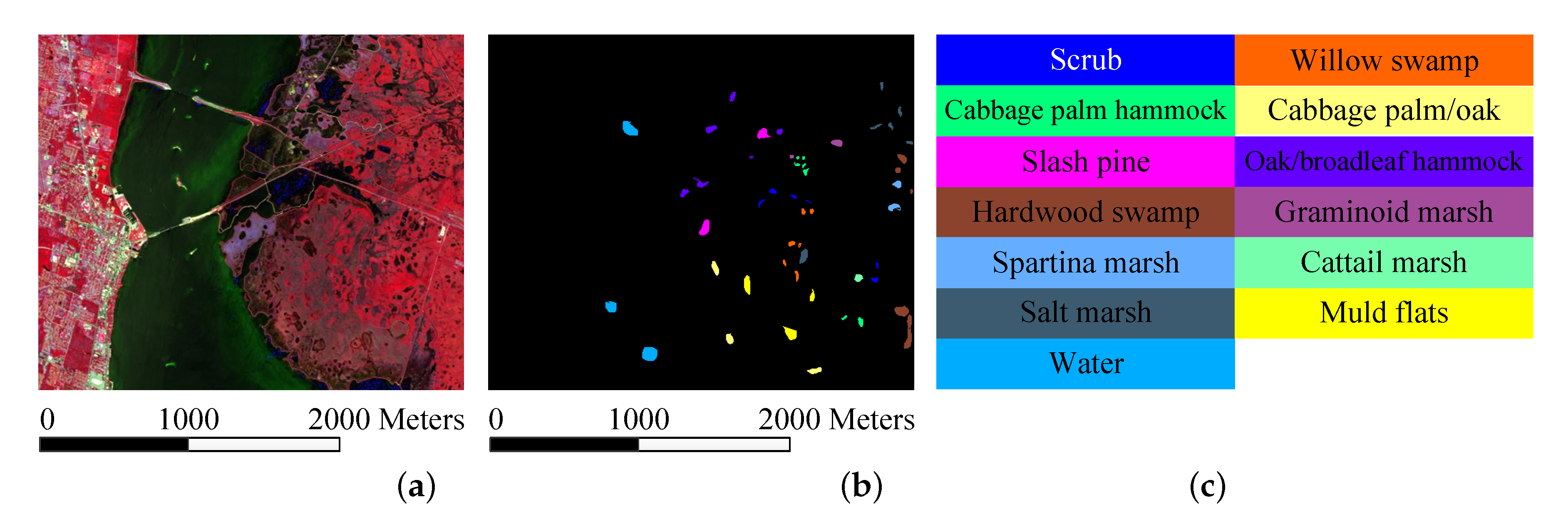
AVIRIS KSC Dataset: The Kennedy Space Center (KSC) image was collected by the AVIRIS sensor over the Kennedy Space Center in Florida. The image is 512 × 614 pixels, where 48 bands have been removed as water absorption and low SNR bands. Figure 4a–c show the false color composite of the Kennedy Space Center image and the reference classification map, which contains 13 different classes. Figure 4 shows that the false-color composite of the KSC image, the corresponding reference data, and the corresponding color code. Table 3 shows the experimental conditions.
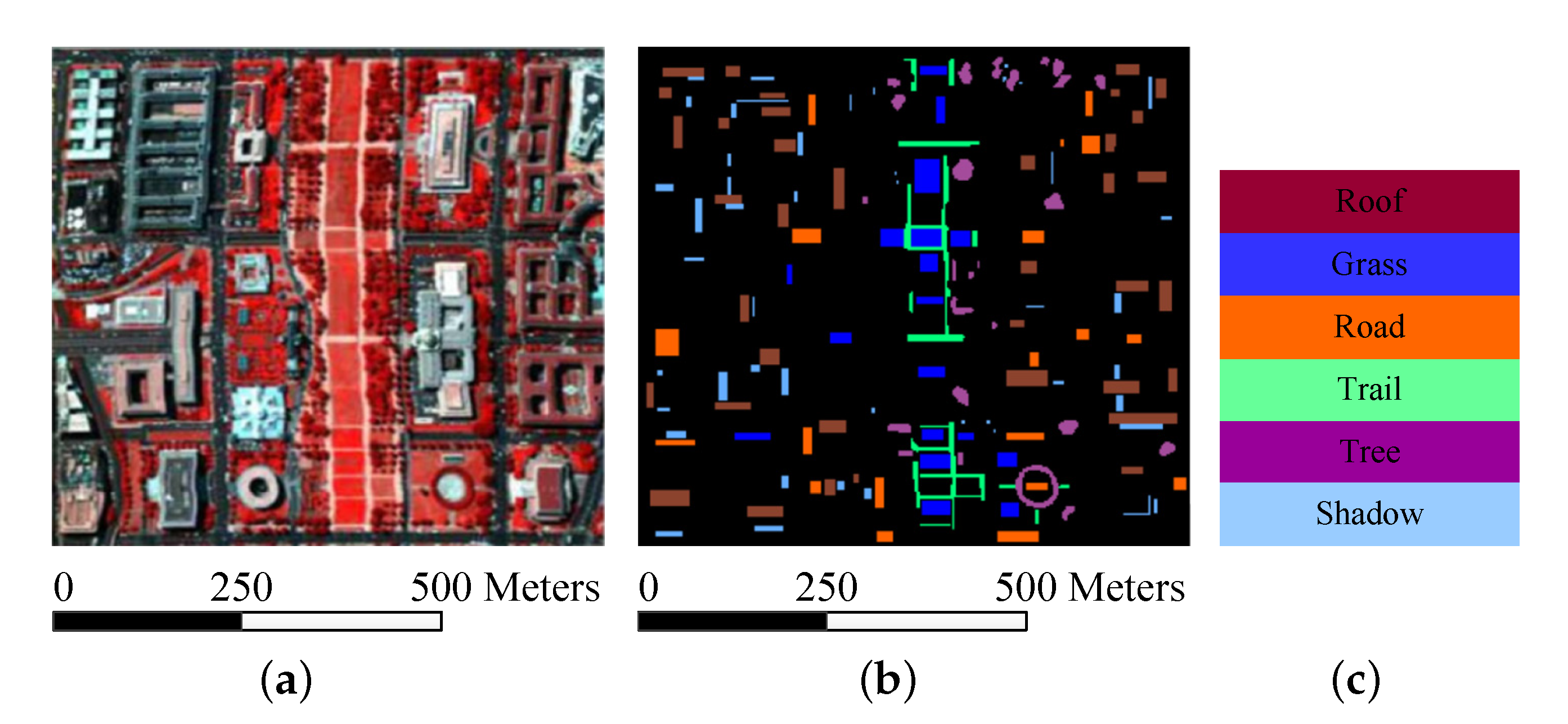
HYDICE Washington DC Dataset: The Washington DC image was collected by the Hyperspectral Digital Image Collection Experiment (HYDICE) sensor over the Washington DC Mall. The sensor system measured 210 bands (for our experiments, 19 bands in the spectral range 0.9–1.4 × 10 μm were omitted) of the visible and infrared spectrum in 0.4–2.4 μm. The dataset contains 280 scan lines, each of which contains 307 pixels. The false-color composite and reference map (containing six ground reference classes) for Washington DC are as shown in Figure 5a–c. Figure 5 shows that the false-color composite of the Washington DC image, the corresponding reference data, and the corresponding color code. The experimental conditions are recorded in Table 4.
As one of the most widely used pixelwise classifiers, this paper adopts the SVM to evaluate the performance of the proposed KECA method, which is implemented with the LIBSVM library [45] using the radial basis function kernel. Moreover, the parameters of the SVM are determined using fivefold cross-validation. To make the comparison fair, the represented quality indexes of the overall accuracy (OA), average accuracy (AA), Kappa coefficient (Kappa), and class individual accuracies are calculated by averaging the results achieved in ten repeated Monte Carlo experiments with different randomly selected training samples and noisy labels, and the mean and standard deviation in repeated experiments of the accuracies are represented in experimental reports. The training sets are constructed using samples in the ground truth. For each class, some pixels randomly selected from other classes will be added to simulate the “noisy label" problem.
4.2. Parameter Tuning
This section starts by analyzing the influence of the parameter on the performance of the proposed KECA method. Figure 6 gives the experimental results achieved for the University of Pavia, Salinas, KSC, and Washington DC dataset, respectively. For the University of Pavia dataset, 50 true samples and ten noisy labels are selected randomly for each class. For the Salinas, KSC, and Washington DC dataset 25 true samples and five noisy labels are selected randomly for each class. The size of the kernel parameter is set with intervals 0.02–0.22. As shown in Figure 6, it can be observed that the classification accuracy rises first and then falls. The reason is that the width parameter controls the radial range of the RBF kernel. Taking Figure 6a, a too large or too small radial range can lead to performance degradation of the proposed method. When the is set to 0.12, the classification accuracy achieves 81.10%. For the Salinas, KSC, and Washington DC dataset, the highest classification accuracies will be obtained when is set to 0.1, 0.12, 0.18, respectively. Specifically, = 0.13 is suggested to be used as the default parameters in the proposed method when the proposed KECA method is conducted on a new dataset.
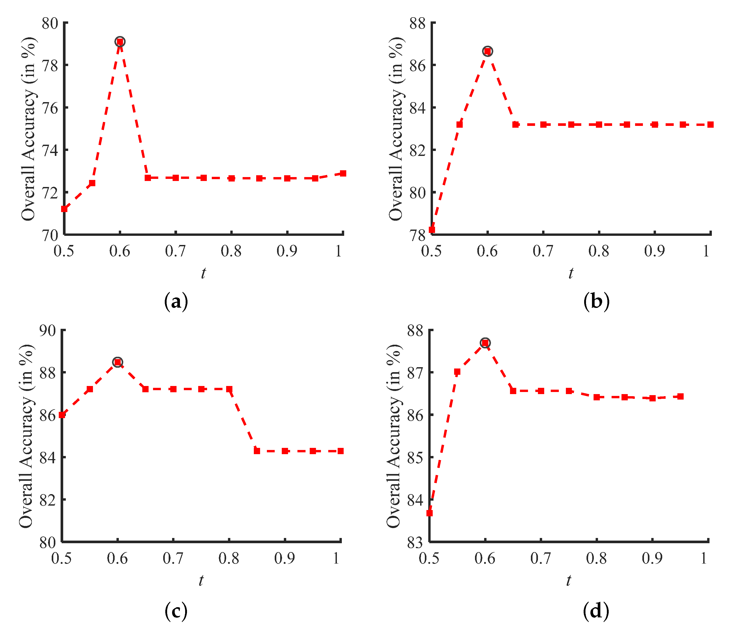
The second experiment sought to analyze the effectiveness of the threshold parameter t. The experiment is conducted on the University of Pavia dataset with 50 true samples and ten noisy labels per class, the Salinas dataset with 25 true samples and five noisy labels per class, the KSC dataset with 25 true samples and five noisy labels per class, and the Washington DC dataset with 25 true samples and five noisy labels per class, respectively. Moreover, the range of the parameter t is set to 0.5–1. Based on the experimental results presented in Figure 7, it can be found that the optimal classification accuracies can be obtained by the proposed KECA method when the t is set to 0.6. The reason is that the values of t control the number of noisy labels to be removed. If the t value is too small, the noisy labels in the training set will not be cleaned, whereas an excessive t value will remove true samples in the training set. Therefore, the threshold parameter t = 0.6 is set to default parameters in the proposed method according to the highest classification accuracy of the SVM trained using that training set that has been improved by the proposed KECA method. Similarly, if given a new dataset, applying a default of t = 0.6 for parameter is suggested in the proposed method.
In addition, the proposed KECA method may achieve better performance when using optimization procedure for setting [46]. However, KECA only involves two important parameters in performing the noisy labels detection process. Using the optimal parameter setting based on the experimental results can effectively reduce the time cost due to automatic tuning. Therefore, in order to balance the detection accuracy and time validity, we adopted the experimental optimal parameter setting in the subsequent experiments.
4.3. Component Analysis
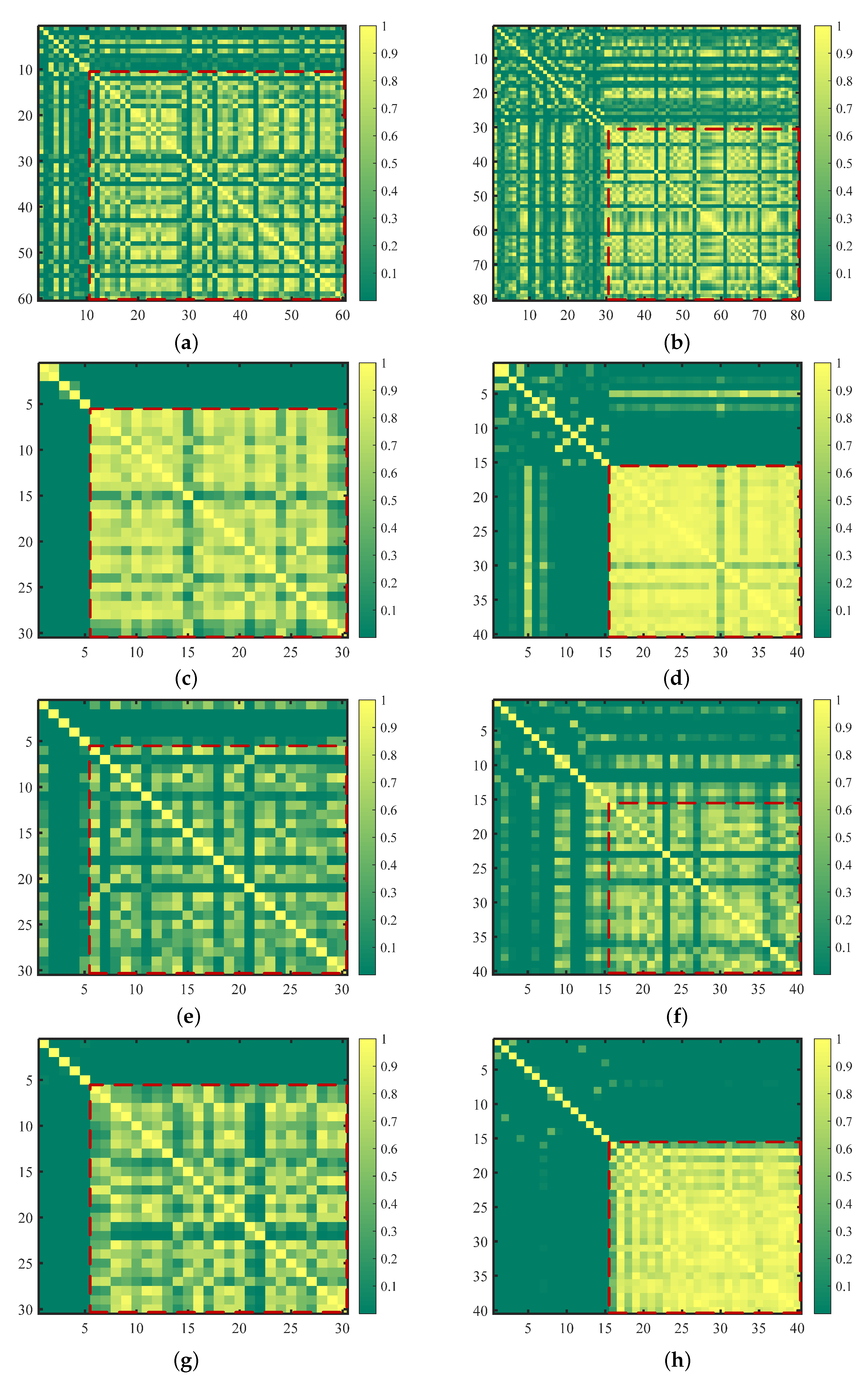
Here, an experiment is performed on the KSC dataset with 25 true training samples and five noisy labels per class, in which the performance of the proposed method with different kernel trick such linear kernel function (LKF), polynomial kernel function (PKF), wavlet kernel function (WKF), Laplacian kernel function (LNKF), and radial basis function (RBF), is analyzed in Table 5. We can observe from Table 5 that the proposed RBF-based KECA method achieves the best performance in terms of classification accuracies. Therefore, the RBF kernel trick is adopted for the proposed method and used in the following experiments. In addition, to further demonstrate the effectiveness of the RBF kernel in the proposed method, the illustration of the RBF-based kernel matrix in different classes of the four hyperspectral real datasets is given in Figure 8. Evidently, the RBF kernel-based discrimination between true samples and noisy labels is pretty obvious (see outside the red dotted box). Focusing on Figure 8c,d, it can be observed that good septation between true samples and noisy labels still exist when the original training set contains a larger of mislabeled samples. Specifically, the difference is more pronounced in the Salinas, KSC, and Washington DC datasets. This means that the RBF kernel can be an effective component of the proposed method for noisy label detection in supervised HSI classification tasks.
4.4. Detection Performance Analysis
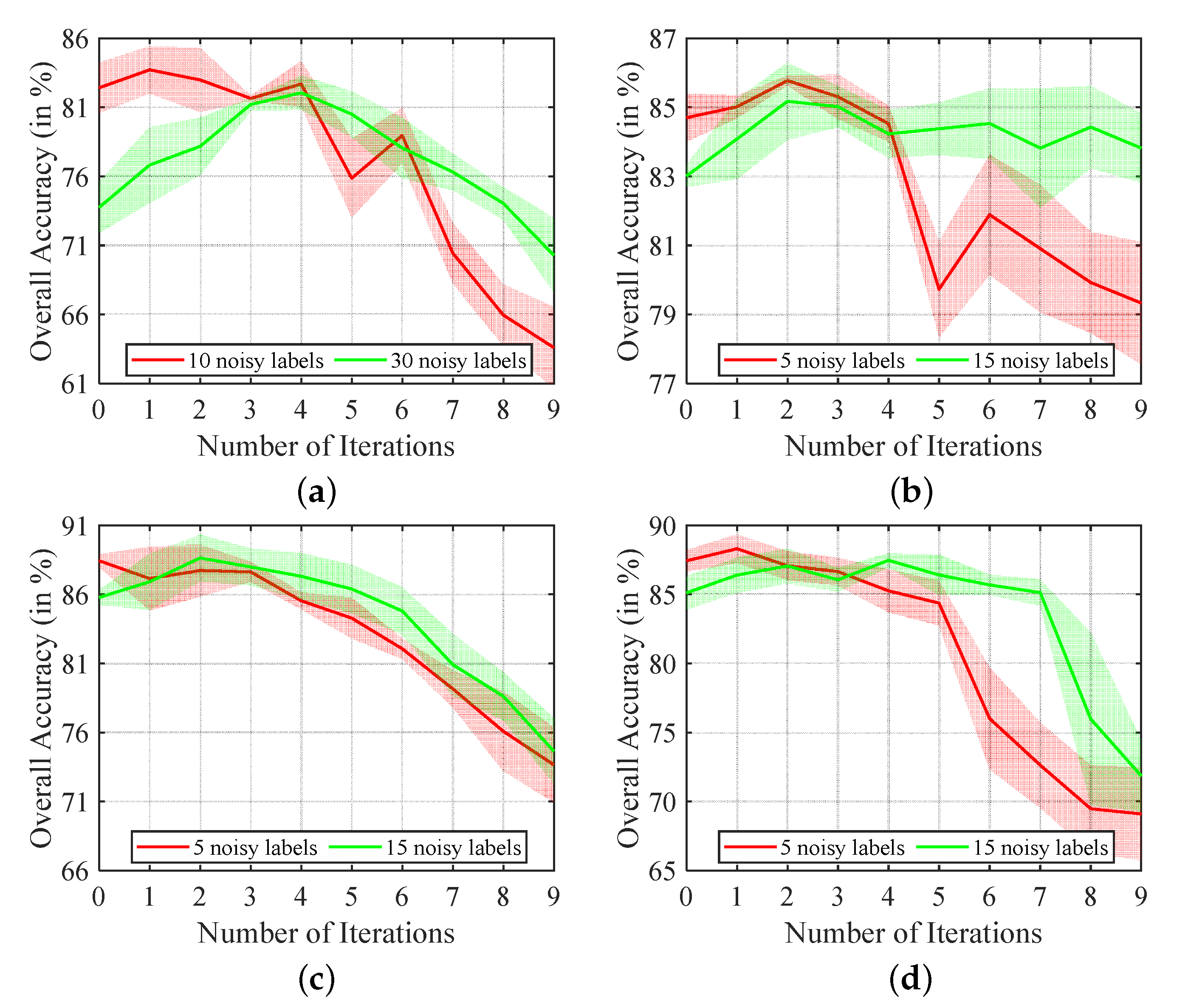
In this section, the first experiment is performed to analyze the influence of the number of iterations on the performance of the proposed KECA method. For the University of Pavia dataset, the noisy original training set contains 50 true samples and different numbers of noisy labels for each class. For the KSC, Salinas, and Washington DC scenes, the training sets each contain 25 true samples and various noisy labels for each class. The main iteration steps in the proposed method is to repeat Equations (10)–(19) and the main idea of iteration is that the previous output can be used as the next input until the stop criterion has been satisfied. As shown in Table 6, it can be found that the proposed KECA method achieves a low false detection rate (see the third column), which means that only a few true samples were detected as false. However, the improved training set still contains some noisy labels (fourth column), particularly, when a large number of noisy labels still exist in the original training set. The reason is that decision threshold-based removal solution is dissatisfied with the original training set that has a large number of noisy labels. Therefore, the iteration detection of proposed method is introduced into the improved training set to further remove noisy labels. As shown in Figure 9, it can be seen that the OA decreases as the number of iterations increases when the original training set has few noise labels (see the red curve) on the different HSI datasets. However, when a training set contains more noise labels (see the green curve), the OAs rise and then fall with the number of iterations. Therefore, iteration detection can achieve better detection accuracy in a training set with many noisy labels. Taking into account the balance between calculation efficiency and classification accuracy, the number of iterations of the proposed method is set to one for HSI datasets in this paper.
4.5. Performance Evaluation Using the SVM
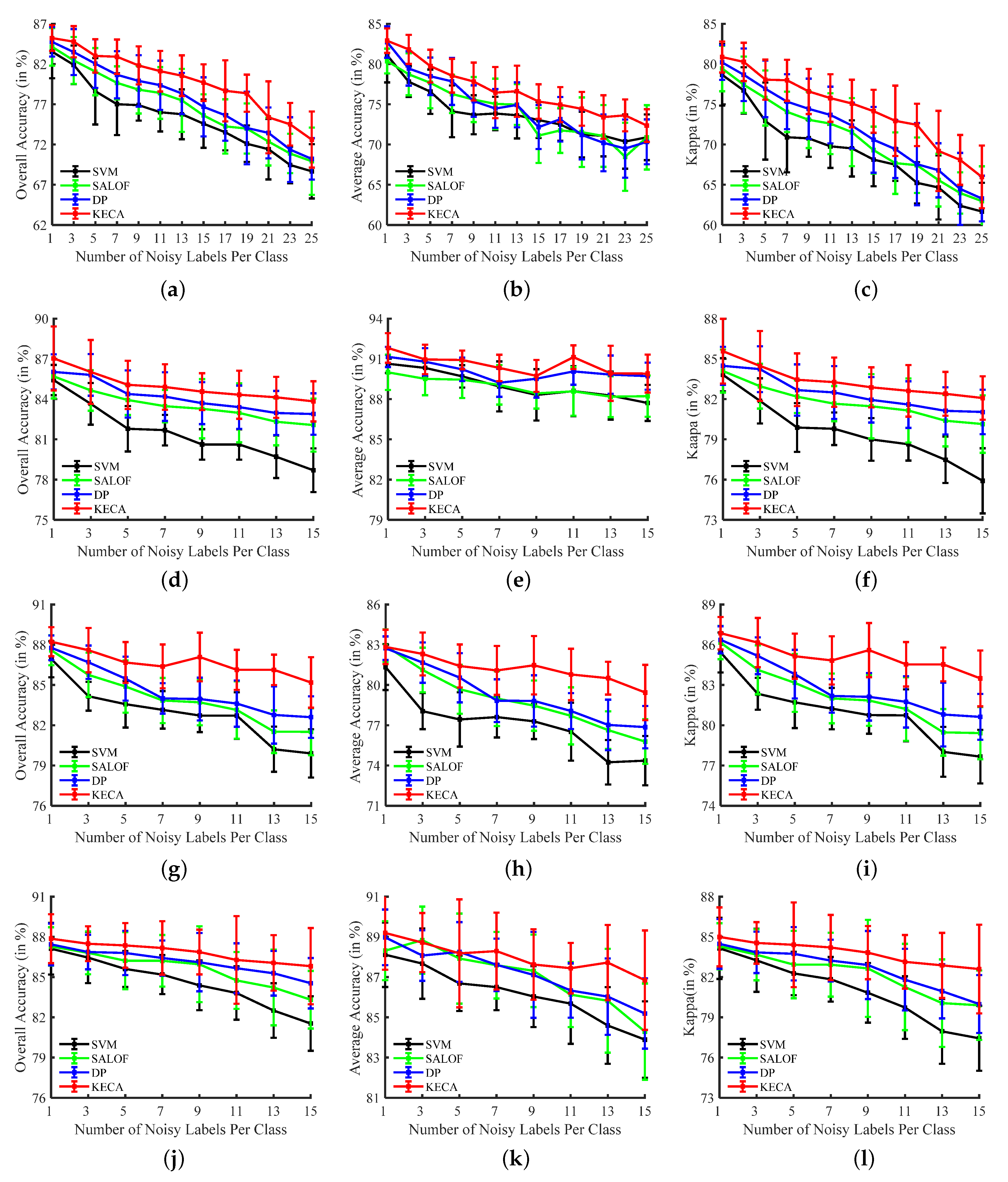
In this section, the classification results of different methods, such as the SVM, SALOF, DP, and the proposed KECA method, are evaluated by the SVM trained with different improved training sets on the University of Pavia, KSC, Salinas, and Washington DC datasets. For the University of Pavia dataset, experiments are conducted with 50 true samples and 1–25 noisy labels per class. For the KSC, Salinas, and Washington DC datasets, the experiments are conducted with 25 true samples and 1–15 noisy labels per class. Figure 10 shows the classification performance of the SVM trained using the different training sets, which represented the average values and the standard deviation of the obtained OAs, AAs, and Kappas across ten repeated experiments. The SVM trained with the improved training sets are higher than the original training set. Specifically, the SVM trained using the training set improved by KECA can always achieve optimal classification results compared to the training set improved by other detection methods in terms of OA, AA, and Kappa. Therefore, introducing kernel trick based entropy component analysis can further improve the detection accuracy of noisy labels and the classification performance of the SVM.
In addition, Table 7 contains the classification results for University of Pavia dataset, it shows that the proposed KECA method can effectively improve the classification accuracies for the most classes. For instance, when a training set contains 30 noisy labels for each class, the classification accuracy of the SVM trained using that training set improved by the KECA training set increases from 80.15% to 91.10% for the asphalt class and from 70.81% to 90.45% for shadows class compared to the other improved training sets. Meanwhile, the OAs can be promoted by approximately 5%. This demonstrates that the noisy labels in the original training set can be effectively removed by the proposed KECA method with respect to the SALOF and DP methods.
Table 8 and Figure 11 represent the classification results for the Salinas dataset. As shown in Table 8, when the original training set contains five noisy labels for each class, the SVM trained using training set improved by the KECA is promoted by about 4% in terms of the classification accuracy (i.e., OA) with respect to the SVM trained using the original training set. Similarly, the classification accuracy of the SVM is obviously promoted using the training set improved by the KECA (by about 5%). In addition, the SVM trained using the training set improved by the KECA achieves better classification results in terms of OA, AA, and Kappa compared to the SVM trained using the training set improved by other method such as SALOF or DP. As shown in Figure 11, It can be observed that the classification results of fallow smooth and vineyard trellis achieved by the SVM trained with the noisy training set show serious misclassification. By comparison, such misclassification can obviously be reduced in the classification results obtained by the SVM trained with a training set improved by the KECA. Specifically, the classification results of the SVM trained with the training set improved by the KECA show significant improvements compared to the SVM trained with training set cleansed by other methods. Furthermore, it has been demonstrated that the proposed KECA method can effectively cleanse the noisy training set and improve the supervised classification performance in HSI.
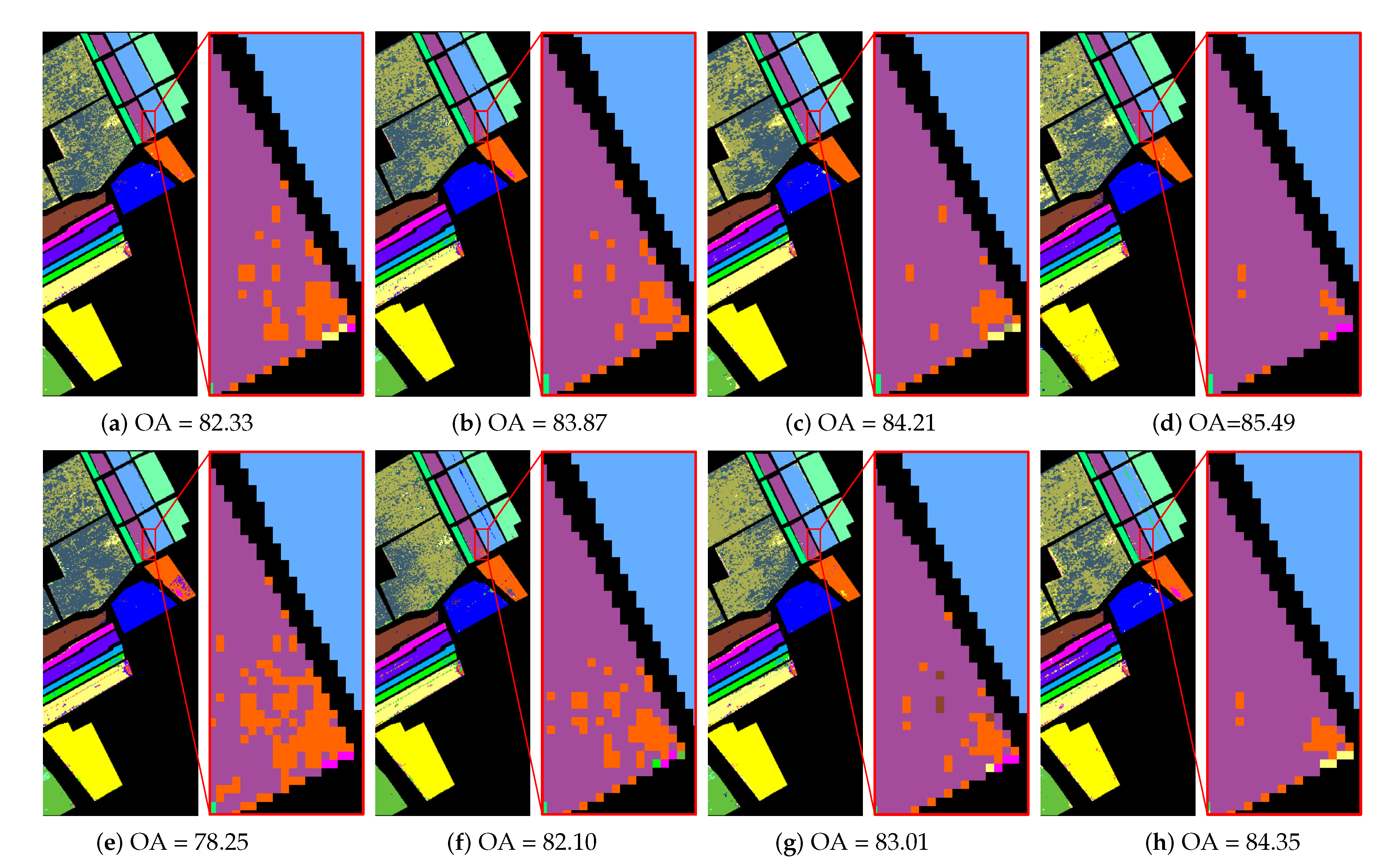
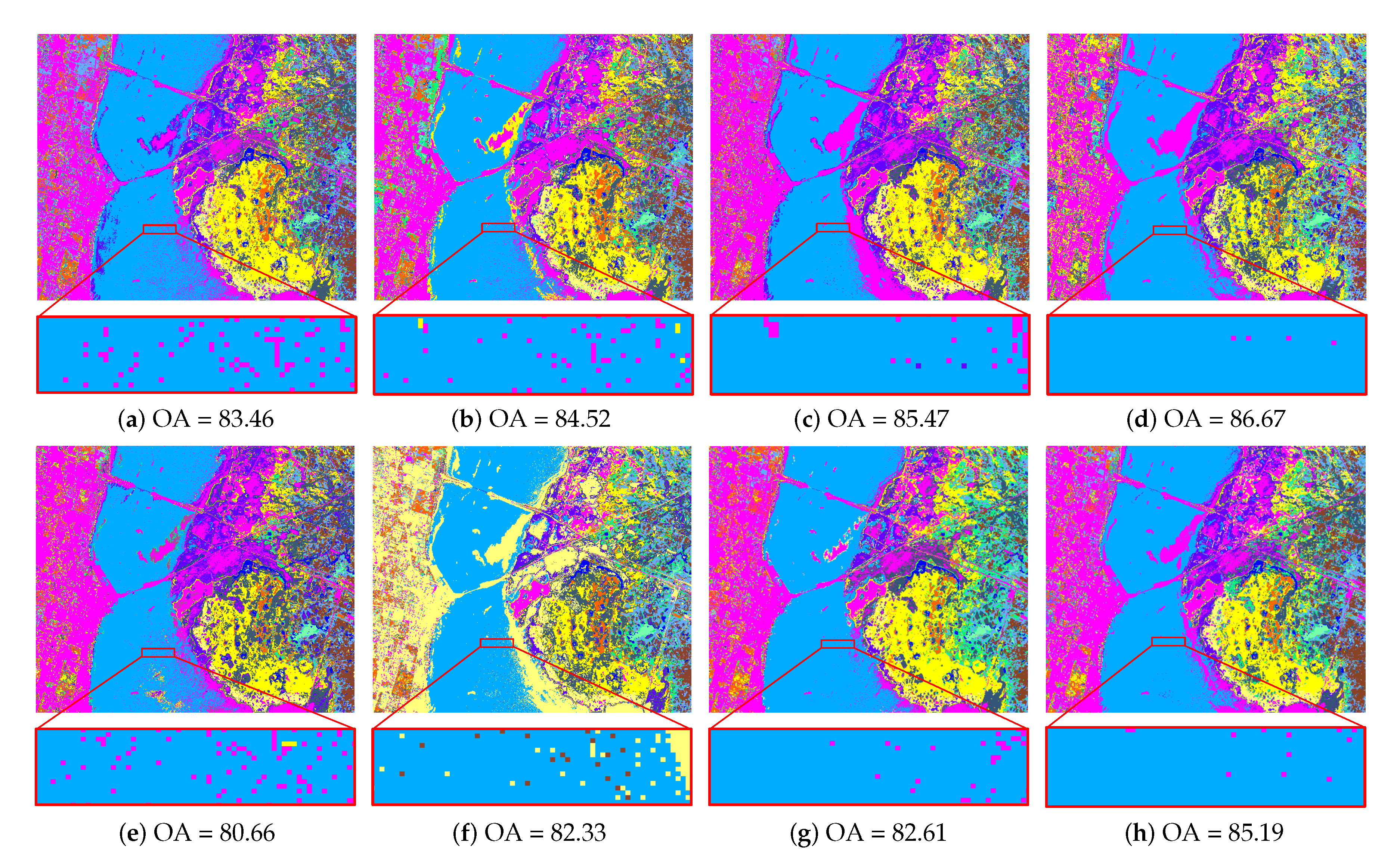
Table 9 and Figure 12 present the experimental results of the KSC data set. As shown in Table 9, when the number of the noisy labels increases, the classification performance of the proposed KECA method becomes more obviously promoted in terms of OAs, AAs, and Kappas with respect to the other methods. For instance, when the original training set contains 25 true samples and five noisy labels per class, the classification accuracy can be improved approximately 3% by applying the proposed noisy label detection method. When the rate of noisy labels becomes 50%, the amount of improvement in classification accuracies reaches 5%. Specifically, the classification accuracy of the KECA improvement is significantly greater than that of the comparison method (see Table 9). As shown in the local window comparisons presented in Figure 12, the classification results achieved by the proposed KECA method are more similar to the reference data (see Figure 4b). Besides the University of Pavia, Salinas, and KSC datasets, the proposed method has been performed on the Washington DC datasets to further demonstrate the effectiveness of the KECA in HSI noisy label detection. Table 10 contains the classification results. The proposed method can improve the accuracies by 1.75–6.47%. Therefore, the proposed KECA method has the robustness of increasing the classification accuracy in HSI supervised tasks.
Finally, Table 11 shows the time-consumption (in seconds) for the different of methods to classify the four real HSI datasets. All codes are conducted on a computer with an Intel(R) Core(TM) i5-7300HQ, CPU 2.50 GHz CPU, and 8 GB of RAM, and the software platform is MATLAB R2019a (MathWorks, Natick, Massachusetts, America). As shown in Table 11, the time-consumption improvement for the SVM trained using a training set with the proposed method was less than the SVM trained using the original noisy training set. In addition, the proposed KECA method has run-time advantages over the SALOF and DP methods in most simulations. This shows that the proposed method can effectively detect and remove noisy labels form a training set, and thus reduce the training time for the SVM. Besides the time spent on classification, Table 11 show the detection time of the different detection methods. The proposed KECA method typically needed less time to execute detection processing with noisy labels compared to the competitive methods. This phenomenon can demonstrate the effectiveness and robustness of the proposed KECA method.
4.6. Performance Evaluation Using Other Classifiers
In this section, the performance of the proposed KECA method is evaluated by employing some widely used spectral classifiers, such as the basic thresholding classifier (BTC) [47], the kernel basic thresholding classifier (KBTC) [42], the sparse representation classifier (SRC) [48], and the extreme learning machine (ELM) [49], to demonstrate the effectiveness of the proposed noisy label detection method. In this experiment, the proposed KECA method is conducted on the Salinas dataset with 25 true training samples and different numbers of noisy labels for each class. To make the competition more objective, the experiment was repeated ten times to obtain the average value and the standard deviation of the classification accuracies. As shown in Table 12, the classification accuracies of different spectral classifiers trained with the original training set and the training set improved by different noisy label detection methods are represented, respectively. It can be seen that the spectral classifiers using the improved training set always obtain better classification accuracies with respect to those trained with the original noisy training set. Specifically, the classification accuracies of the spectral classifiers trained using the training set cleansed by the KECA often achieve higher classification results than the spectral classifiers trained using training set cleansed by the competitive methods in the term of OAs, AAs, and Kappas. It is demonstrated that the proposed KECA method can be widely employed in supervised hyperspectral processing tasks to promote the accuracy of spectral classifiers.
Furthermore, the proposed method is extended to some spectral-spatial classifiers, i.e., representative spectral-spatial classification methods are adopted including extended morphological profiles (EMP) [50], logistic regression and multilevel logistic (LMLL) [51], the joint sparse representation classifier (JSRC) [13], and the edge-preserving filtering (EPF) [52], to prove that the classification performance of a spectral-spatial classifier trained using the training set with different numbers of noisy labels can be improved by exploiting the proposed KECA method. The experiment was also performed on the Salinas dataset with 25 true training samples and different numbers of noisy labels for each class. Similarly, the experiments are repeated ten times to obtain the results of fair competition. Table 13 shows that the classification accuracies of a spectral-spatial classifier trained using the original training set are much lower than those trained with the corrected training sets. In particular, when the number of noisy labels increases, the effectiveness of the proposed KECA method in terms of accuracy is more obvious than competitive methods such as the SALOF and DP methods. This experiment further demonstrates that the proposed method can effectively detect and remove noisy labels, and it is also useful for improving the performance of spectral-spatial classifiers.
5. Discussion on Feature Extraction
In this section, to further illustrate that the proposed method under different feature methods, i.e., linear discriminant analysis (LDA), principal component analysis (PCA), recursive filter (RF), and extended morphological profiles (EMPs), can effectively detect and remove noisy labels in the training set, an experimental analysis of detection performance is conducted on the KSC datasets with 25 true samples and five noisy labels per class. As shown in Table 14, it can be observed that the EMP-based KECA obtains better OA, AA, Kappa with respect to other features. This means that significant features can further improve the detection performance of the proposed KECA method. However, taking into account the versatility of the KECA method, the report presented by our paper is the experimental result of the original spectral features.
6. Conclusions and Future Lines
This paper first proposes kernel entropy component analysis to cleanse a noisy training set in supervised HSI classification. The key idea of this work is exploiting kernel-based entropy distribution to detect noisy labels in the original training set. Experimental results conducted on several real hyperspectral scenes show the effectiveness of the proposed methods in terms of classification evaluations. However, one limitation of the proposed method is that it has not taken into account the contextual information of the training samples in the detection process. Therefore, utilizing the kernel-based spectral and spatial information of hyperspectral data to further promote the detection performance will be an important research topic in our future work.
Author Contributions
B.T. and C.Z. designed the proposed model and implemented the experiments. C.Z. and X.O. drafted the manuscript. J.P. and Z.X. worked on the improvement of tho proposed model and edited the manuscript. B.T. and W.H. provided overall guidance to the project, reviewed and edited the manuscript, and obtained funding to support this research.
Funding
This research received no external funding.
Acknowledgments
This work was supported in part by the National Natural Science Foundation of China under Grants 61977022 and 51704115, by the Natural Science Foundation of Hunan Province under Grants 2019JJ50212, 2019JJ50211, 2017JJ2107, and 2018JJ2155, by the Hunan Provincial Innovation Foundation for Postgraduate under Grants CX2018B771 and CX20190914, by the Key Research and Development Program of Hunan Province und Grant 2019SK2102, by the Hunan Emergency Communication Engineering Technology Research Center under Grant 2018TP2022, by the Engineering Research Center on 3D Reconstruction and Intelligent Application Technology of Hunan Province under Grant 2019-430602-73-03-006049, and by the Scientific Research Program of Hunan Province Education Department under Grant 17C0174.
Conflicts of Interest
The authors declare no conflict of interest.
References
- Ellis, R.J.; Scott, P.W. Evaluation of hyperspectral remote sensing as a means of environmental monitoring in the St. Austell China clay (kaolin) region, Cornwall, UK. Remote Sens. Environ. 2004, 93, 118–130. [Google Scholar] [CrossRef]
- Pullanagari, R.R.; Kereszturi, G.; Yule, I. Integrating airborne hyperspectral, topographic, and soil data for estimating pasture quality using recursive feature elimination with random forest regression. Remote Sens. 2018, 10, 1117. [Google Scholar] [CrossRef]
- Erives, H.; Fitzgerald, G.J. Automated registration of hyperspectral images for precision agriculture. Comput. Electron. Agric. 2005, 47, 103–119. [Google Scholar] [CrossRef]
- Herrmann, I.; Vosberg, S.K.; Ravindran, P.; Singh, A.; Chang, H.X.; Chilvers, M.I.; Conley, S.P.; Townsend, P.A. Leaf and canopy level detection of fusarium virguliforme (sudden death syndrome) in soybean. Remote Sens. 2018, 10, 426. [Google Scholar] [CrossRef]
- Bishop, C.A.; Liu, J.G.; Mason, P.J. Hyperspectral remote sensing for mineral exploration in Pulang, Yunnan Province, China. Int. J. Remote Sens. 2011, 32, 2409–2426. [Google Scholar] [CrossRef]
- Jackisch, R.; Lorenz, S.; Zimmermann, R.; Möckel, R.; Gloaguen, R. Drone-borne hyperspectral monitoring of acid mine drainage: an example from the sokolov lignite district. Remote Sens. 2018, 10, 385. [Google Scholar] [CrossRef]
- Tu, B.; Yang, X.; Li, N.; Zhou, C.; He, D. Hyperspectral anomaly detection via density peak clustering. Pattern Recognit. Lett. 2020, 129, 144–149. [Google Scholar] [CrossRef]
- Melgani, F.; Bruzzone, L. Classification of hyperspectral remote sensing images with support vector machines. IEEE Trans. Geosci. Remote Sens. 2004, 42, 1778–1790. [Google Scholar] [CrossRef]
- Wang, Y.; Duan, H. Classification of hyperspectral images by SVM using a composite kernel by employing spectral, spatial and hierarchical structure information. Remote Sens. 2018, 10, 441. [Google Scholar] [CrossRef]
- Zhu, X.; Li, N.; Pan, Y. Optimization performance comparison of three different group intelligence algorithms on a SVM for hyperspectral imagery classification. Remote Sens. 2019, 11, 734. [Google Scholar] [CrossRef]
- Xia, J.; Chanussot, J.; Du, P.; He, X. Rotation-based support vector machine ensemble in classification of hyperspectral data with limited training samples. IEEE Trans. Geosci. Remote Sens. 2015, 54, 1519–1531. [Google Scholar] [CrossRef]
- Pal, M.; Foody, G.M. Feature selection for classification of hyperspectral data by SVM. IEEE Trans. Geosci. Remote Sens. 2010, 48, 2297–2307. [Google Scholar] [CrossRef]
- Yi, C.; Nasrabadi, N.M.; Tran, T.D. Hyperspectral image classification using dictionary-based sparse representation. IEEE Trans. Geosci. Remote Sens. 2011, 49, 3973–3985. [Google Scholar]
- Yuan, Y.; Lin, J.; Wang, Q. Hyperspectral image classification via multitask joint sparse representation and stepwise MRF optimization. IEEE Trans. Cybern. 2016, 46, 2966–2977. [Google Scholar] [CrossRef]
- Zhang, E.; Zhang, X.; Jiao, L.; Lin, L.; Hou, B. Spectral-spatial hyperspectral image ensemble classification via joint sparse representation. Pattern Recognit. 2016, 59, 42–54. [Google Scholar] [CrossRef]
- Fei, T.; Tong, H.; Jiang, J.; Yun, Z. Multiscale union regions adaptive sparse representation for hyperspectral image classification. Remote Sens. 2017, 9, 872. [Google Scholar]
- Fang, L.; Zhuo, H.; Li, S. Super-resolution of hyperspectral image via superpixel-based sparse representation. Neurocomputing 2018, 273, 171–177. [Google Scholar] [CrossRef]
- Tu, B.; Huang, S.; Fang, L.; Zhang, G.; Wang, J.; Zheng, B. Hyperspectral image classification via weighted joint nearest neighbor and sparse representation. IEEE J. Sel. Top. Appl. Earth Obs. Remote Sens. 2018, 11, 4063–4075. [Google Scholar] [CrossRef]
- Liu, L.; Chen, L.; Chen, C.L.P.; Tang, Y.Y.; Pun, C.M. Weighted joint sparse representation for removing mixed noise in image. IEEE Trans. Cybern. 2017, 47, 600–611. [Google Scholar] [CrossRef]
- Liu, Y.F.; Guo, J.M.; Lee, J.D. Halftone image classification using LMS algorithm and naive bayes. IEEE Trans. Image Process. 2011, 20, 2837–2847. [Google Scholar]
- Wang, X.Z.; He, Y.L.; Wang, D.D. Non-naive bayesian classifiers for classification problems with continuous attributes. IEEE Trans. Cybern. 2013, 44, 21–39. [Google Scholar] [CrossRef] [PubMed]
- Xu, L.; Li, J. Bayesian classification of hyperspectral imagery based on probabilistic sparse representation and markov random field. IEEE Trans.Geosci. Remote Sens. 2014, 11, 823–827. [Google Scholar]
- Safavian, S.R.; Landgrebe, D. A survey of decision tree classifier methodology. IEEE Trans. Syst. Man Cybern. 2002, 21, 660–674. [Google Scholar] [CrossRef]
- Yang, C.C.; Prasher, S.O.; Enright, P.; Madramootoo, C.; Burgess, M.; Goel, P.K.; Callum, I. Application of decision tree technology for image classification using remote sensing data. Agric. Syst. 2003, 76, 1101–1117. [Google Scholar] [CrossRef]
- Moustakidis, S.P.; Mallinis, G.; Koutsias, N.; Theocharis, J.B.; Petridis, V. SVM-based fuzzy decision trees for classification of high spatial resolution remote sensing images. IEEE Trans. Geosci. Remote Sens. 2011, 50, 149–169. [Google Scholar] [CrossRef]
- Li, S.; Hao, Q.; Gao, G.; Kang, X. The effect of ground truth on performance evaluation of hyperspectral image classification. IEEE Trans. Geosci. Remote Sens. 2018, 56, 7195–7206. [Google Scholar] [CrossRef]
- Garcia-Vilchez, F.; Munoz-Mari, J.; Zortea, M.; Blanes, I.; Gonzalez-Ruiz, V.; Camps-Valls, G.; Plaza, A.; Serra-Sagrista, J. On the impact of lossy compression on hyperspectral image classification and unmixing. IEEE Geosci. Remote Sens. Lett. 2011, 8, 253–257. [Google Scholar] [CrossRef]
- Carlotto, M.J. Effect of errors in ground truth on classification accuracy. Int. J. Remote Sens. 2009, 30, 4831–4849. [Google Scholar] [CrossRef]
- Tu, B.; Yang, X.; Li, N.; Ou, X.; He, W. Hyperspectral image classification via superpixel correlation coefficient representation. IEEE J. Sel. Top. Appl. Earth Obs. Remote Sens. 2018, 11, 4113–4127. [Google Scholar] [CrossRef]
- Xiao, T.; Xia, T.; Yang, Y.; Huang, C.; Wang, X. Learning from massive noisy labeled data for image classification. In Proceedings of the IEEE Conf. Comput. Vis. Pattern Recognit (CVPR), Boston, MA, USA, 7–12 June 2015; pp. 2691–2699. [Google Scholar]
- Lu, Z.; Fu, Z.; Xiang, T.; Han, P.; Wang, L.; Gao, X. Learning from weak and noisy labels for semantic segmentation. IEEE Trans. Pattern Anal. Mach. Intell. 2017, 39, 486–500. [Google Scholar] [CrossRef]
- Yao, Y.; Wang, L.; Zhang, L.; Yang, Y.; Li, P.; Zimmermann, R.; Shao, L. Learning latent stable patterns for image understanding with weak and noisy labels. IEEE Trans. Cybern. 2019, 49, 4243–4252. [Google Scholar] [CrossRef] [PubMed]
- Kang, X.; Duan, P.; Xiang, X.; Li, S.; Benediktsson, J.A. Detection and correction of mislabeled training samples for hyperspectral image classification. IEEE Trans. Geosci. Remote Sens. 2018, 56, 5673–5686. [Google Scholar] [CrossRef]
- Jiang, J.; Ma, J.; Wang, Z.; Chen, C.; Liu, X. Hyperspectral image classification in the presence of noisy labels. IEEE Trans. Geosci. Remote Sens. 2019, 57, 851–865. [Google Scholar] [CrossRef]
- Tu, B.; Zhou, C.; Kuang, W.; Guo, L.; Ou, X. Hyperspectral imagery noisy label detection by spectral angle local outlier factor. IEEE Geosci. Remote Sens. Lett. 2018, 15, 1417–1421. [Google Scholar] [CrossRef]
- Tu, B.; Zhang, X.; Kang, X.; Zhang, G.; Li, S. Density peak-based noisy label detection for hyperspectral image classification. IEEE Trans. Geosci. Remote Sens. 2019, 57, 1573–1584. [Google Scholar] [CrossRef]
- Tu, B.; Zhang, X.; Kang, X.; Wang, J.; Benediktsson, J.A. Spatial density peak clustering for hyperspectral image classification with noisy labels. IEEE Trans. Geosci. Remote Sens. 2019, 57, 5085–5097. [Google Scholar] [CrossRef]
- Jie, L.; Yuan, Q.; Shen, H.; Zhang, L. Noise removal from hyperspectral image with joint spectral–spatial distributed sparse representation. IEEE Trans. Geosci. Remote Sens. 2016, 54, 5425–5439. [Google Scholar]
- He, L.; Pan, Q.; Di, W.; Li, Y. Anomaly detection in hyperspectral imagery based on maximum entropy and nonparametric estimation. Pattern Recognit. Lett. 2008, 29, 1392–1403. [Google Scholar] [CrossRef]
- Cheng, C.; Hao, X.; Liu, S. Image segmentation based on 2D Renyi gray entropy and fuzzy clustering. In Proceedings of the IEEE Int. Conf. Signal Process, Hangzhou, China, 19–23 October 2014; pp. 19–23. [Google Scholar]
- Jie, F.; Jiao, L.; Tao, S.; Liu, H.; Zhang, X. Multiple kernel learning based on discriminative kernel clustering for hyperspectral band selection. IEEE Trans. Geosci. Remote Sens. 2016, 54, 6516–6530. [Google Scholar]
- Toksz, M.A.; Ulusoy, I. Hyperspectral image classification via kernel basic thresholding classifier. IEEE Trans. Geosci. Remote Sens. 2017, 55, 715–728. [Google Scholar] [CrossRef]
- Li, J.; Marpu, P.R.; Plaza, A.; Bioucas-Dias, J.M.; Benediktsson, J.A. Generalized composite kernel framework for hyperspectral image classification. IEEE Trans. Geosci. Remote Sens. 2013, 51, 4816–4829. [Google Scholar] [CrossRef]
- Fang, L.; Li, S.; Duan, W.; Ren, J.; Benediktsson, J.A. Classification of hyperspectral images by exploiting spectral–spatial information of superpixel via multiple kernels. IEEE Trans. Geosci. Remote Sens. 2015, 53, 6663–6674. [Google Scholar] [CrossRef] [Green Version]
- Chang, C.C.; Lin, C.J. LIBSVM: A library for support vector machines. ACM Trans. Intell. Syst. Technol. 2011, 2, 27:1–27:27. [Google Scholar] [CrossRef]
- Ding, X.; Zhang, S.; Li, H.; Wu, P.; Dale, P.; Liu, L.; Cheng, S. A restrictive polymorphic ant colony algorithm for the optimal band selection of hyperspectral remote sensing images. Int. J. Remote Sens. 2020, 41, 1093–1117. [Google Scholar] [CrossRef]
- Toksz, M.A.; Ulusoy, I. Hyperspectral image classification via basic thresholding classifier. IEEE Trans. Geosci. Remote Sens. 2016, 54, 4039–4051. [Google Scholar] [CrossRef]
- Wright, J.; Yang, A.Y.; Ganesh, A.; Sastry, S.S.; Ma, Y. Robust face recognition via sparse representation. IEEE Trans. Pattern Anal. Mach. Intell. 2009, 31, 210–227. [Google Scholar] [CrossRef] [Green Version]
- Huang, G.-B.; Zhou, H.; Ding, X.; Zhang, R. Extreme learning machine for regression and multiclass classification. IEEE Trans. Syst. Man Cybern. 2012, 42, 513–529. [Google Scholar] [CrossRef]
- Benediktsson, J.A.; Pesaresi, M.; Amason, K. Classification and feature extraction for remote sensing images from urban areas based on morphological transformations. IEEE Trans. Geosci. Remote Sens. 2003, 41, 1940–1949. [Google Scholar] [CrossRef] [Green Version]
- Li, J.; Bioucas-Dias, J.M.; Plaza, A. Hyperspectral image segmentation using a new Bayesian approach with active learning. IEEE Trans. Geosci. Remote Sens. 2011, 49, 3947–3960. [Google Scholar] [CrossRef] [Green Version]
- Kang, X.; Li, S.; Benediktsson, J.A. Spectral-spatial hyperspectral image classification with edge-preserving filtering. IEEE Trans. Geosci. Remote Sens. 2014, 52, 2666–2677. [Google Scholar] [CrossRef]
Figure 1.
Illustrating the framework of the proposed KECA method to detect noisy labels.

Figure 2.
University of Pavia data set. (a) three-band color composite; (b) reference data; (c) color code.
Figure 2.
University of Pavia data set. (a) three-band color composite; (b) reference data; (c) color code.

Figure 3.
Salinas data set. (a) three-band color composite; (b) reference data; (c) color code.

Figure 4.
KSC data set. (a) three-band color composite; (b) reference data; (c) color code.

Figure 5.
Washington DC data set. (a) three-band color composite; (b) reference data; (c) color code.
Figure 5.
Washington DC data set. (a) three-band color composite; (b) reference data; (c) color code.

Figure 6.
Influence of the parameters k on the proposed KECA method. (a) University of Pavia dataset with 50 true samples and ten noisy labels for each class; (b) Salinas dataset with 25 true samples and five noisy labels for each class; (c) KSC dataset with 25 true samples and five noisy labels for each class; (d) Washington DC dataset with 25 true samples and five noisy labels for each class.

Figure 7.
Effect of parameters k on the performance of the proposed KECA method. (a) University of Pavia dataset with 50 true samples and ten noisy labels per class; (b) Salinas dataset with 25 true samples and five noisy labels per class; (c) KSC dataset with 25 true samples and five noisy labels per class; (d) Washington DC dataset with 25 true samples and five noisy labels per class.

Figure 8.
Illustration of the RBF-based kernel matrix in different classes for the four hyperspectral real datasets. (a,b) University of Pavia (50 true samples and ten/thirty noisy labels); (c,d) Salinas (25 true samples and five/fifteen noisy labels); (e,f) KSC (25 true samples and five/fifteen noisy labels); (g,h) Washington DC (25 true samples and five/fifteen noisy labels).

Figure 9.
Classification accuracy achieved by the KECA with different numbers of iterations. (a) The University of Pavia dataset; (b) The Salinas dataset; (c) The KSC dataset; (d) The Washington DC dataset.
Figure 9.
Classification accuracy achieved by the KECA with different numbers of iterations. (a) The University of Pavia dataset; (b) The Salinas dataset; (c) The KSC dataset; (d) The Washington DC dataset.

Figure 10.
Performance comparison between the SVM trained using the original training sets and when using the improved training sets obtained by the SALOF, DP, and, KECA methods in terms of OA (first column), AA (second column), and Kappa (third column). (a–c) experiments on the University of Pavia data set with different numbers of mislabeled (in the range 1–25) and 50 true samples for each class; (d–f) experiments on the KSC data set with different number of mislabeled (in the range 1–15) and 25 true samples for each class; (g–i) experiments on the Salinas data set with different numbers of mislabeled (in the range 1–15) and 25 true samples for each class; (j–l) experiments on the Washington DC data set with different numbers of mislabeled (in the range 1–15) and 25 true samples for each class.

Figure 11.
Classification results (%) of the various methods with the University of Pavia dataset. Classification maps obtained by the SVM (first column), DP (second column), SALOF methods (third column), and the proposed KECA method (fifth column) trained with 50 true samples and different numbers of noisy labels per class: (a–d) 10 noisy labels per class, and (e–h) 30 noisy labels per class.

Figure 12.
Classification results (%) of different methods on the KSC dataset. Classification maps obtained by the SVM (first column), DP (second column), SALOF methods (third column), and the proposed KECA method (fifth column) trained with 25 true samples and different numbers of noisy labels per class: (a–d) 5 noisy labels per class, and (e–h) 15 noisy labels per class.


Table 1.
Number of samples, i.e., training samples, test samples, and noisy labels, of nine classes in the University of Pavia data set.
Table 1.
Number of samples, i.e., training samples, test samples, and noisy labels, of nine classes in the University of Pavia data set.
| Class | Name | Train | Test | Added noise labels | |
|---|---|---|---|---|---|
| Exp. 1 | Exp. 2 | ||||
| C1 | Asphalt | 50 | 6581 | 10 | 30 |
| C2 | Meadows | 50 | 18,599 | 10 | 30 |
| C3 | Gravel | 50 | 2049 | 10 | 30 |
| C4 | Trees | 50 | 3014 | 10 | 30 |
| C5 | Metal sheets | 50 | 1295 | 10 | 30 |
| C6 | Bare soil | 50 | 4979 | 10 | 30 |
| C7 | Bitumen | 50 | 1280 | 10 | 30 |
| C8 | Self-Blocking Bricks | 50 | 3632 | 10 | 30 |
| C9 | Shadows | 50 | 897 | 10 | 30 |
| Total | 450 | 42,326 | 90 | 270 | |
Table 2.
Number of samples, i.e., training samples, test samples, and noisy labels, of sixteen classes in the Salinas data set.
Table 2.
Number of samples, i.e., training samples, test samples, and noisy labels, of sixteen classes in the Salinas data set.
| Class | Name | Train | Test | Added Noisy Labels | |
|---|---|---|---|---|---|
| Exp. 1 | Exp. 2 | ||||
| C1 | Weeds 1 | 25 | 1984 | 5 | 15 |
| C2 | Weeds 2 | 25 | 3701 | 5 | 15 |
| C3 | Fallow | 25 | 1951 | 5 | 15 |
| C4 | Fallow plot | 25 | 1369 | 5 | 15 |
| C5 | Fallow smooth | 25 | 2653 | 5 | 15 |
| C6 | Stubble | 25 | 3934 | 5 | 15 |
| C7 | Celery | 25 | 3554 | 5 | 15 |
| C8 | Grapes | 25 | 11,246 | 5 | 15 |
| C9 | Soil | 25 | 6178 | 5 | 15 |
| C10 | Corn | 25 | 3253 | 5 | 15 |
| C11 | Lettuce 4 wk | 25 | 1043 | 5 | 15 |
| C12 | Lettuce 5 wk | 25 | 1902 | 5 | 15 |
| C13 | Lettuce 6 wk | 25 | 891 | 5 | 15 |
| C14 | Lettuce 7 wk | 25 | 1045 | 5 | 15 |
| C15 | Vinyard untrained | 25 | 7243 | 5 | 15 |
| C16 | Vinyard trelis | 25 | 1782 | 5 | 15 |
| Total | 400 | 53,729 | 80 | 240 | |
Table 3.
Number of samples, i.e., training samples, test samples, and noisy labels, of thirteen classes in the Salinas data set.
Table 3.
Number of samples, i.e., training samples, test samples, and noisy labels, of thirteen classes in the Salinas data set.
| Class | Name | Train | Test | Added Noise Labels | |
|---|---|---|---|---|---|
| Exp. 1 | Exp. 2 | ||||
| C1 | Scrub | 25 | 736 | 5 | 15 |
| C2 | Willow swamp | 25 | 218 | 5 | 15 |
| C3 | Cabbage palm hammock | 25 | 231 | 5 | 15 |
| C4 | Cabbage palm/oak | 25 | 227 | 5 | 15 |
| C5 | Slash pine | 25 | 136 | 5 | 15 |
| C6 | Oak/broadleaf hammock | 25 | 204 | 5 | 15 |
| C7 | Hardwood swamp | 25 | 80 | 5 | 15 |
| C8 | Graminoid marsh | 25 | 406 | 5 | 15 |
| C9 | Spartina marsh | 25 | 495 | 5 | 15 |
| C10 | Cattail marsh | 25 | 379 | 5 | 15 |
| C11 | Salt marsh | 25 | 394 | 5 | 15 |
| C12 | Muld flats | 25 | 478 | 5 | 15 |
| C13 | Water | 25 | 902 | 5 | 15 |
| Total | 325 | 4886 | 65 | 195 | |
Table 4.
Number of samples, i.e., training samples, test samples, and noisy labels, of six classes in the Washington DC data set.
Table 4.
Number of samples, i.e., training samples, test samples, and noisy labels, of six classes in the Washington DC data set.
| Class | Name | Train | Test | Added Noise Labels | |
|---|---|---|---|---|---|
| Exp. 1 | Exp. 2 | ||||
| C1 | Roof | 25 | 3160 | 5 | 15 |
| C2 | Grass | 25 | 1797 | 5 | 15 |
| C3 | Road | 25 | 1403 | 5 | 15 |
| C4 | Trail | 25 | 1262 | 5 | 15 |
| C5 | Tree | 25 | 1190 | 5 | 15 |
| C6 | Shadow | 25 | 1115 | 5 | 15 |
| Total | 150 | 9927 | 30 | 90 | |
Table 5.
Classification performance obtained by the KECA method using different kernel tricks for the KSC dataset with 25 true samples and five noisy labels for each class. Number in the parenthesis represents the standard variance of the accuracies obtained in repeat experiments.
Table 5.
Classification performance obtained by the KECA method using different kernel tricks for the KSC dataset with 25 true samples and five noisy labels for each class. Number in the parenthesis represents the standard variance of the accuracies obtained in repeat experiments.
| Class | SVM 25 (T) | SVM 25 (T) + 5(M) | The Different Kernel Tricks Based KECA Method | ||||
|---|---|---|---|---|---|---|---|
| LKF | PKF | WKF | LNKF | RBF | |||
| C1 | 94.92(2.47) | 93.53(2.22) | 95.03(1.59) | 94.67(1.74) | 95.86(1.61) | 94.72(1.83) | 95.10(1.45) |
| C2 | 89.05(4.36) | 79.86(5.84) | 84.89(5.68) | 83.97(4.09) | 78.45(11.0) | 84.77(4.60) | 87.20(5.17) |
| C3 | 87.57(6.11) | 91.84(4.62) | 87.71(5.43) | 83.27(6.68) | 82.22(6.27) | 83.69(6.13) | 85.96(3.79) |
| C4 | 67.59(5.56) | 58.72(4.06) | 66.80(5.35) | 63.49(3.08) | 57.27(6.78) | 63.95(5.29) | 64.87(6.15) |
| C5 | 65.38(7.52) | 51.88(9.44) | 63.74(8.07) | 60.46(7.49) | 57.37(9.73) | 61.38(7.85) | 64.95(7.23) |
| C6 | 61.91(8.81) | 51.72(6.18) | 58.73(5.82) | 55.37(8.30) | 54.88(12.0) | 58.18(7.28) | 60.98(7.30) |
| C7 | 71.02(5.58) | 56.83(6.80) | 65.13(6.16) | 67.22(6.52) | 63.81(5.85) | 67.02(6.77) | 67.44(4.60) |
| C8 | 84.20(6.37) | 82.58(8.09) | 83.27(5.33) | 82.91(6.12) | 70.84(12.0) | 82.99(5.00) | 83.43(6.94) |
| C9 | 90.42(2.27) | 89.27(2.87) | 89.03(3.87) | 88.35(2.98) | 83.56(6.38) | 89.32(2.63) | 89.22(2.29) |
| C10 | 93.02(7.52) | 80.85(7.23) | 94.27(5.85) | 93.60(4.39) | 86.01(10.8) | 96.72(3.46) | 93.08(6.84) |
| C11 | 90.08(5.48) | 86.72(5.45) | 90.29(4.46) | 91.46(4.59) | 93.53(7.89) | 90.07(5.16) | 90.09(6.90) |
| C12 | 94.77(3.61) | 83.62(4.44) | 92.74(3.59) | 93.08(5.38) | 86.73(7.43) | 95.49(2.70) | 95.02(3.65) |
| C13 | 100.0(0.00) | 99.18(0.81) | 99.06(1.39) | 98.88(1.22) | 99.54(0.63) | 99.69(0.65) | 99.69(0.46) |
| OA | 88.75(0.96) | 83.57(1.74) | 87.69(1.24) | 86.77(0.96) | 83.14(2.47) | 87.62(1.11) | 88.05(1.24) |
| AA | 83.84(1.23) | 77.43(2.03) | 82.36(1.68) | 81.29(1.01) | 77.70(2.58) | 82.15(1.31) | 82.85(1.47) |
| Kappa | 87.45(1.06) | 81.71(1.93) | 86.27(1.38) | 85.25(1.06) | 81.22(2.74) | 86.20(1.23) | 86.67(1.38) |
Table 6.
Detection performance (numbers) of noisy labels for the proposed method on a different dataset. Note that the experimental results is the average of ten repeated experiments for objective evaluation. Here, represents the total number of noisy labels in the training set, refers to the number of noisy labels per class, and the number in parentheses represents the standard variance of the accuracies obtained in repeated experiments.
| Datasets | Total Noises | Evaluation of Detection Performance of Noise Labels | ||||
|---|---|---|---|---|---|---|
| Correct | Error | Not Detected | Correct Rate (%) | Error Rate (%) | ||
| University of Pavia | 10 × 9 | 54.53(3.16) | 2.60(1.24) | 35.47(3.16) | 60.07(3.81) | 2.89(1.34) |
| 30 × 9 | 107.27(4.04) | 0.00(0.00) | 162.73(4.04) | 39.90(2.20) | 0.00(0.00) | |
| Salinas | 5 × 16 | 54.90(3.38) | 15.50(3.75) | 25.10(3.38) | 70.75(2.96) | 19.38(3.14) |
| 15 × 16 | 142.90(6.81) | 0.10(0.32) | 97.10(6.81) | 61.67(2.28) | 0.01(0.01) | |
| KSC | 5 × 13 | 45.10(2.81) | 11.50(2.68) | 19.90(2.81) | 68.46(3.01) | 17.69(4.98) |
| 15×13 | 150.50(4.55) | 9.10(2.64) | 44.50(4.55) | 76.87(1.72) | 4.93(1.97) | |
| Washington DC | 5 × 6 | 20.50(1.65) | 5.20(2.10) | 9.50(1.65) | 69.67(5.76) | 17.33(4.22) |
| 15 × 6 | 58.50(2.64) | 2.64(0.40) | 31.50(2.64) | 65.78(4.44) | 2.94(0.57) | |
Table 7.
Classification performance of the SVM, SALOF, DP, and KECA methods for the University of Pavia dataset with 50 true samples and different number of noisy labels per class as training set. The number in the parenthesis represents the standard variance of the accuracies obtained over repeat experiments.
| Class | SVM 50 (T) | The Number of True Samples and Noisy Labels Per Class | |||||||
|---|---|---|---|---|---|---|---|---|---|
| 50 (True) + 10 (Noise) | 50 (True) + 30 (Noise) | ||||||||
| SVM | SALOF | DP | KECA | SVM | SALOF | DP | KECA | ||
| C1 | 94.98 | 90.51(3.74) | 92.13(5.61) | 86.54(6.60) | 93.83(2.93) | 80.15(11.0) | 88.60(5.89) | 88.84(7.29) | 91.10(6.18) |
| C2 | 94.68 | 92.60(1.22) | 93.24(1.24) | 94.05(1.80) | 94.66(1.25) | 91.85(2.24) | 90.49(2.72) | 92.35(2.39) | 92.81(1.51) |
| C3 | 66.61 | 55.22(6.42) | 65.42(4.97) | 58.34(6.34) | 60.75(6.77) | 50.80(6.57) | 53.50(5.85) | 52.75(6.20) | 54.88(5.32) |
| C4 | 80.73 | 69.77(7.40) | 73.01(7.33) | 81.01(9.36) | 73.04(10.2) | 67.06(8.60) | 63.18(9.77) | 57.25(10.4) | 64.06(8.57) |
| C5 | 95.18 | 85.9(11.94) | 81.55(15.6) | 82.64(12.3) | 86.01(11.2) | 76.43(19.6) | 78.63(14.3) | 84.25(9.59) | 85.43(12.9) |
| C6 | 67.05 | 53.49(6.21) | 53.05(5.05) | 65.03(9.61) | 66.78(7.79) | 44.18(6.77) | 42.34(7.26) | 44.72(5.76) | 45.16(6.36) |
| C7 | 61.71 | 49.24(6.74) | 58.61(6.94) | 47.13(5.44) | 51.71(7.17) | 40.42(3.27) | 44.77(4.28) | 42.93(5.38) | 43.65(5.11) |
| C8 | 82.13 | 77.34(5.49) | 81.03(4.23) | 71.67(6.69) | 75.89(5.29) | 70.40(6.29) | 77.58(4.53) | 80.56(3.69) | 76.22(6.58) |
| C9 | 99.92 | 90.61(9.02) | 77.4(13.75) | 83.8(16.93) | 88.34(14.6) | 70.81(19.2) | 73.5(22.48) | 88.16(10.4) | 90.45(12.7) |
| OA | 85.06 | 76.01(2.39) | 78.40(3.21) | 79.36(3.06) | 81.11(2.53) | 66.48(3.76) | 67.87(5.41) | 69.92(3.30) | 71.00(4.07) |
| AA | 82.56 | 73.85(2.07) | 75.05(3.13) | 74.47(2.41) | 76.77(3.18) | 65.79(4.85) | 68.07(4.17) | 70.20(2.95) | 71.53(3.22) |
| Kappa | 80.61 | 69.77(2.67) | 72.59(3.78) | 73.67(3.52) | 75.77(2.96) | 59.36(3.93) | 60.83(5.65) | 63.00(3.62) | 64.28(4.34) |
Table 8.
Classification performance of the SVM, SALOF, DP, and KECA methods for the Salinas dataset with 25 true samples and different numbers of noisy labels per class as a training set. The number in the parentheses represents the standard variance of the accuracies obtained over repeated experiments.
| Class | SVM 25 (T) | The Number of True Samples and Noisy Labels | |||||||
|---|---|---|---|---|---|---|---|---|---|
| 25 (True) + 5 (Noise) | 25 (True) + 15 (Noise) | ||||||||
| SVM | SALOF | DP | KECA | SVM | SALOF | DP | KECA | ||
| C1 | 98.80 | 98.87(2.27) | 99.41(0.75) | 98.78(1.47) | 94.40(7.19) | 98.90(0.92) | 96.32(4.00) | 98.88(1.03) | 96.63(3.99) |
| C2 | 99.22 | 99.33(0.92) | 99.17(0.55) | 99.33(0.24) | 94.14(3.99) | 94.65(1.24) | 97.59(2.56) | 98.29(1.34) | 98.09(2.38) |
| C3 | 99.66 | 90.24(2.44) | 90.79(2.41) | 88.47(4.08) | 91.86(1.99) | 91.72(3.84) | 88.31(2.91) | 89.35(2.61) | 88.31(3.43) |
| C4 | 97.57 | 97.38(0.96) | 97.20(0.70) | 97.26(0.44) | 93.86(3.87) | 97.03(1.77) | 93.68(7.78) | 95.91(2.10) | 94.46(4.42) |
| C5 | 98.52 | 98.18(1.63) | 98.54(1.02) | 98.75(0.74) | 99.37(1.34) | 94.70(4.20) | 98.15(1.39) | 98.05(2.07) | 98.85(4.45) |
| C6 | 100.0 | 99.44(2.43) | 100.0(0.00) | 100.0(0.00) | 99.95(0.13) | 99.77(2.74) | 100.0(0.00) | 98.17(2.13) | 98.54(2.36) |
| C7 | 98.47 | 98.57(1.53) | 98.58(0.89) | 98.56(1.03) | 96.82(2.82) | 96.96(1.62) | 96.10(5.06) | 97.49(1.61) | 98.25(1.05) |
| C8 | 74.03 | 71.15(3.13) | 72.03(2.39) | 72.67(2.65) | 75.37(3.83) | 59.59(4.24) | 71.02(4.44) | 70.70(3.66) | 73.39(2.70) |
| C9 | 99.22 | 99.27(0.68) | 99.22(0.35) | 99.28(0.29) | 98.66(1.06) | 99.42(0.65) | 98.98(0.74) | 98.51(2.08) | 99.59(3.42) |
| C10 | 80.00 | 77.35(6.60) | 79.84(9.54) | 78.32(5.34) | 82.32(7.69) | 84.80(4.97) | 84.44(5.65) | 81.33(7.25) | 80.73(6.93) |
| C11 | 85.46 | 87.78(3.26) | 85.95(5.98) | 88.42(7.22) | 83.89(7.68) | 83.47(5.86) | 88.73(4.44) | 88.15(4.77) | 85.47(5.14) |
| C12 | 94.81 | 92.28(2.02) | 95.08(1.71) | 95.52(1.45) | 96.46(1.13) | 95.07(2.92) | 94.09(3.22) | 94.66(1.37) | 95.51(3.44) |
| C13 | 93.48 | 92.58(4.54) | 90.42(6.95) | 94.00(1.93) | 94.74(3.78) | 95.19(5.78) | 92.03(6.53) | 91.96(3.35) | 91.02(5.47) |
| C14 | 90.97 | 91.68(6.06) | 85.56(11.2) | 88.18(11.3) | 89.61(5.29) | 53.79(10.3) | 79.27(14.7) | 89.20(9.30) | 90.83(7.61) |
| C15 | 58.13 | 47.47(3.85) | 54.31(3.85) | 54.72(5.41) | 57.05(5.50) | 37.16(7.63) | 50.18(5.47) | 50.87(4.91) | 53.49(4.08) |
| C16 | 95.79 | 93.52(4.95) | 85.09(13.7) | 91.17(9.27) | 95.22(2.59) | 89.21(6.64) | 82.57(13.9) | 93.80(7.58) | 94.87(5.45) |
| OA | 85.81 | 81.79(1.69) | 83.94(1.12) | 84.38(1.76) | 85.06(1.79) | 78.29(2.23) | 82.07(1.98) | 82.89(1.54) | 83.83(1.50) |
| AA | 90.95 | 89.69(0.83) | 89.45(1.37) | 90.21(0.87) | 90.24(0.70) | 85.71(1.34) | 88.22(1.54) | 89.71(1.01) | 89.89(1.42) |
| Kappa | 84.24 | 79.88(1.82) | 82.18(1.21) | 82.67(1.91) | 83.44(1.97) | 75.91(2.42) | 80.14(2.14) | 81.04(1.66) | 82.08(1.62) |
Table 9.
Classification performance of the SVM, SALOF, DP, and KECA methods for the KSC dataset with 25 true samples and different numbers of noisy labels per class as the training set. The number in the parentheses represents the standard variance of the accuracies obtained in repeat experiments.
Table 9.
Classification performance of the SVM, SALOF, DP, and KECA methods for the KSC dataset with 25 true samples and different numbers of noisy labels per class as the training set. The number in the parentheses represents the standard variance of the accuracies obtained in repeat experiments.
| Class | SVM 25 (T) | The Number of True Samples and Noisy Labels | |||||||
|---|---|---|---|---|---|---|---|---|---|
| 25 (True) + 5 (Noise) | 25 (True) + 15 (Noise) | ||||||||
| SVM | SALOF | DP | KECA | SVM | SALOF | DP | KECA | ||
| C1 | 94.92 | 93.53(2.22) | 95.90(1.79) | 95.30(1.78) | 93.29(2.70) | 96.11(2.93) | 95.43(2.19) | 95.19(2.10) | 93.38(2.14) |
| C2 | 89.05 | 79.86(5.84) | 83.34(5.33) | 83.77(4.17) | 85.60(4.97) | 77.02(5.08) | 74.58(5.21) | 74.53(6.08) | 79.93(6.27) |
| C3 | 87.57 | 91.84(4.62) | 85.19(5.65) | 84.55(4.21) | 82.76(5.90) | 86.19(6.20) | 84.14(5.72) | 84.34(6.03) | 81.06(7.49) |
| C4 | 67.59 | 58.72(4.06) | 64.28(6.09) | 64.64(4.57) | 62.60(4.92) | 56.02(4.67) | 55.63(7.01) | 57.00(6.80) | 60.02(6.45) |
| C5 | 65.38 | 51.88(9.44) | 62.20(5.91) | 61.92(6.14) | 62.45(5.92) | 57.14(9.85) | 52.38(10.6) | 57.82(9.01) | 56.72(8.96) |
| C6 | 61.91 | 51.72(6.18) | 54.59(5.55) | 57.08(6.92) | 55.13(11.5) | 36.10(8.09) | 50.07(7.70) | 48.74(7.39) | 57.81(7.05) |
| C7 | 71.02 | 56.83(6.80) | 68.49(4.32) | 70.00(5.23) | 66.96(7.38) | 53.19(6.30) | 63.78(4.00) | 65.48(6.97) | 60.36(8.86) |
| C8 | 84.20 | 82.58(8.09) | 79.89(5.36) | 78.09(4.85) | 80.34(5.60) | 52.58(10.4) | 66.88(5.54) | 69.17(5.34) | 80.82(6.67) |
| C9 | 90.42 | 89.27(2.87) | 86.95(6.50) | 84.96(4.45) | 89.07(2.09) | 88.55(5.69) | 85.28(7.84) | 82.63(5.88) | 86.75(3.77) |
| C10 | 93.02 | 80.85(7.23) | 83.85(8.77) | 92.55(3.71) | 94.48(5.11) | 83.21(7.67) | 83.16(10.3) | 87.27(10.4) | 94.13(6.35) |
| C11 | 90.08 | 86.72(5.45) | 86.37(9.38) | 87.33(5.23) | 92.60(5.76) | 97.78(4.37) | 88.79(8.51) | 90.71(8.60) | 90.83(4.72) |
| C12 | 94.77 | 83.62(4.44) | 86.77(6.58) | 90.24(5.32) | 93.48(3.59) | 82.76(5.75) | 86.28(8.69) | 87.10(9.22) | 92.81(5.17) |
| C13 | 100.0 | 99.18(0.81) | 98.08(2.24) | 96.62(2.46) | 99.60(0.43) | 100.0(2.18) | 98.73(2.56) | 98.65(2.20) | 98.07(1.99) |
| OA | 88.75 | 83.57(1.74) | 84.88(1.94) | 85.47(1.64) | 86.67(1.52) | 79.90(1.80) | 81.51(1.76) | 82.60(1.55) | 85.19(1.88) |
| AA | 83.84 | 77.43(2.03) | 79.68(1.82) | 80.54(1.83) | 81.42(1.60) | 74.36(1.83) | 75.78(1.67) | 76.86(1.58) | 79.44(2.06) |
| Kappa | 87.45 | 81.71(1.93) | 83.16(2.16) | 83.81(1.82) | 85.14(1.68) | 77.66(2.00) | 79.42(1.95) | 80.62(1.71) | 83.49(2.08) |
Table 10.
Classification performance of the SVM, SALOF, DP, and KECA methods for the Washington DC dataset with 25 true samples and different numbers of noisy labels per class as training set. The number in the parentheses represents the standard variance of the accuracies obtained across repeat experiments.
| Class | SVM 25 (T) | The Number of True Samples and Noisy Labels | |||||||
|---|---|---|---|---|---|---|---|---|---|
| 25 (Ture) + 5 (Noise) | 25 (Ture) + 15 (Noise) | ||||||||
| SVM | SALOF | DP | KECA | SVM | SALOF | DP | KECA | ||
| C1 | 90.28 | 86.08(4.05) | 84.12(4.54) | 88.43(3.57) | 89.28(2.57) | 74.98(5.27) | 84.70(4.43) | 87.45(3.65) | 88.89(3.66) |
| C2 | 95.97 | 95.78(1.26) | 95.63(4.89) | 93.15(3.49) | 95.99(1.76) | 80.04(4.63) | 89.74(5.43) | 89.30(5.82) | 94.25(2.19) |
| C3 | 71.22 | 71.67(3.52) | 70.40(7.23) | 68.80(4.72) | 71.90(4.46) | 68.55(6.71) | 67.30(6.41) | 66.07(5.55) | 69.69(7.37) |
| C4 | 81.67 | 77.41(7.91) | 85.52(6.99) | 83.48(6.80) | 81.95(8.05) | 79.43(7.02) | 76.85(6.71) | 76.95(6.75) | 79.17(7.89) |
| C5 | 95.38 | 93.52(5.00) | 93.48(4.97) | 96.65(5.46) | 96.77(6.80) | 85.62(5.00) | 87.80(6.55) | 94.11(6.17) | 92.98(6.68) |
| C6 | 98.94 | 95.67(7.73) | 98.38(1.59) | 98.99(2.90) | 98.19(7.26) | 96.73(1.80) | 93.35(6.11) | 97.26(2.53) | 96.10(3.55) |
| OA | 87.93 | 85.61(1.33) | 86.22(2.12) | 86.80(1.64) | 87.36(2.67) | 79.34(2.03) | 82.11(2.15) | 83.64(1.88) | 85.81(2.84) |
| AA | 88.91 | 86.69(1.37) | 87.92(2.24) | 88.25(1.48) | 89.01(2.68) | 80.89(1.90) | 83.29(2.39) | 85.19(1.75) | 86.85(2.47) |
| Kappa | 85.14 | 82.27(1.62) | 82.93(2.51) | 83.74(1.99) | 84.41(3.16) | 74.44(2.42) | 78.10(2.58) | 79.99(2.16) | 82.60(3.31) |
Table 11.
Comparison of the time-consumption (in seconds) of various methods. For the University of Pavia dataset, the training set contains 50 true samples and 10 noisy labels per class; the Salinas, KSC, Washington DC dataset contain 25 true samples and 15 noisy labels per class. The Detection Time is marked as DT and the Classification Time is marked as CT.
| Methods | HSI Datasets | |||||||
|---|---|---|---|---|---|---|---|---|
| University of Pavia | Salinas | KSC | Washington DC | |||||
| DT | CT | DT | CT | DT | CT | DT | CT | |
| SVM | − | 45.29 | − | 91.49 | − | 126.22 | − | 17.47 |
| SALOF | 0.42 | 33.30 | 0.16 | 61.87 | 0.11 | 94.71 | 0.07 | 14.79 |
| DP | 0.92 | 36.96 | 0.99 | 66.39 | 0.63 | 58.92 | 0.30 | 10.54 |
| KECA | 0.20 | 26.24 | 0.16 | 74.57 | 0.06 | 87.19 | 0.03 | 11.17 |
Table 12.
Classification Accuracy of the Salinas dataset. The SVM obtained the classification accuracy of 25 true samples and the SVM, SALOF, DP, KECA methods to compare the classification accuracy under 25 true samples and different numbers of noisy labels per class.
Table 12.
Classification Accuracy of the Salinas dataset. The SVM obtained the classification accuracy of 25 true samples and the SVM, SALOF, DP, KECA methods to compare the classification accuracy under 25 true samples and different numbers of noisy labels per class.
| Training Condition | Classifier | OA(%) | AA(%) | Kappa | |||||||||
|---|---|---|---|---|---|---|---|---|---|---|---|---|---|
| SVM | SALOF | DP | KECA | SVM | SALOF | DP | KECA | SVM | SALOF | DP | KECA | ||
| 25(true) + 5(noise) | BTC | 76.23 | 77.76 | 78.90 | 80.15 | 76.35 | 80.78 | 82.66 | 83.37 | 72.77 | 75.44 | 76.69 | 78.06 |
| (1.21) | (1.53) | (1.94) | (1.65) | (0.88) | (1.45) | (2.63) | (1.66) | (1.30) | (1.70) | (1.54) | (1.79) | ||
| KBTC | 75.80 | 80.70 | 82.78 | 85.11 | 76.46 | 85.16 | 87.82 | 89.67 | 73.39 | 78.65 | 80.93 | 83.53 | |
| (1.15) | (2.24) | (1.88) | (1.95) | (1.12) | (2.59) | (1.85) | (2.05) | (1.25) | (2.42) | (2.08) | (2.14) | ||
| SRC | 67.82 | 74.66 | 77.48 | 79.47 | 79.11 | 84.49 | 87.42 | 88.02 | 64.84 | 72.00 | 75.16 | 77.32 | |
| (1.23) | (2.37) | (1.15) | (1.58) | (1.08) | (1.49) | (0.63) | (0.77) | (1.32) | (2.54) | (1.23) | (1.69) | ||
| ELM | 69.54 | 76.17 | 79.72 | 80.74 | 68.98 | 78.00 | 83.48 | 83.53 | 66.67 | 73.79 | 77.63 | 78.45 | |
| (0.98) | (2.17) | (1.36) | (1.72) | (1.42) | (2.39) | (1.55) | (2.25) | (1.05) | (2.34) | (1.45) | (1.84) | ||
| 25(true) + 15(noise) | BTC | 49.46 | 51.62 | 49.33 | 58.99 | 48.13 | 50.53 | 47.88 | 57.94 | 45.66 | 47.60 | 45.07 | 55.31 |
| (1.16) | (2.19) | (1.08) | (2.06) | (1.75) | (2.21) | (1.27) | (2.41) | (1.56) | (2.30) | (1.65) | (2.17) | ||
| KBTC | 57.33 | 62.01 | 61.39 | 67.22 | 55.96 | 60.99 | 61.01 | 66.93 | 53.74 | 58.73 | 58.13 | 64.18 | |
| (1.75) | (1.54) | (1.63) | (1.01) | (1.65) | (1.49) | (1.60) | (1.70) | (1.87) | (1.85) | (1.73) | (1.03) | ||
| SRC | 50.55 | 54.09 | 52.85 | 58.89 | 64.06 | 68.45 | 66.39 | 72.38 | 46.62 | 51.21 | 49.02 | 55.44 | |
| (1.25) | (2.14) | (2.19) | (1.42) | (1.71) | (1.84) | (2.48) | (1.39) | (1.36) | (2.28) | (2.38) | (1.51) | ||
| ELM | 54.38 | 58.13 | 57.84 | 60.76 | 52.63 | 56.43 | 56.11 | 59.32 | 50.64 | 54.71 | 54.43 | 57.41 | |
| (1.52) | (1.54) | (1.86) | (1.55) | (1.15) | (1.52) | (1.96) | (1.38) | (1.59) | (1.65) | (1.90) | (1.64) | ||
| 25(true) + 25(noise) | BTC | 38.93 | 40.39 | 39.80 | 43.69 | 38.05 | 39.28 | 37.83 | 42.62 | 34.28 | 35.72 | 35.04 | 39.13 |
| (0.94) | (1.18) | (1.33) | (1.46) | (1.19) | (1.09) | (0.92) | (1.21) | (1.42) | (1.29) | (1.38) | (1.53) | ||
| KBTC | 46.60 | 50.12 | 49.06 | 54.74 | 45.72 | 49.18 | 48.03 | 53.91 | 42.34 | 46.16 | 45.07 | 50.90 | |
| (1.32) | (1.44) | (1.01) | (1.56) | (1.16) | (1.38) | (0.90) | (1.28) | (1.36) | (1.53) | (1.09) | (1.66) | ||
| SRC | 40.59 | 43.17 | 42.73 | 47.73 | 53.66 | 57.97 | 54.68 | 60.82 | 36.21 | 38.96 | 38.49 | 43.71 | |
| (0.97) | (1.23) | (1.36) | (1.35) | (1.43) | (2.04) | (1.19) | (1.52) | (1.01) | (1.37) | (1.43) | (1.43) | ||
| ELM | 45.81 | 46.70 | 46.80 | 49.35 | 44.49 | 45.76 | 45.29 | 48.01 | 31.65 | 42.68 | 42.70 | 45.39 | |
| (1.20) | (0.79) | (1.19) | (0.90) | (1.14) | (0.87) | (0.88) | (0.81) | (1.25) | (0.90) | (1.22) | (0.98) | ||
Table 13.
Classification Accuracy with the Salinas dataset. The SVM obtained the classification accuracy of 25 true samples and the SVM, SALOF, DP, KECA methods to compare the classification accuracy with 25 true samples and different numbers of noisy labels for each class.
Table 13.
Classification Accuracy with the Salinas dataset. The SVM obtained the classification accuracy of 25 true samples and the SVM, SALOF, DP, KECA methods to compare the classification accuracy with 25 true samples and different numbers of noisy labels for each class.
| Training Condition | Methods | OA(%) | AA(%) | Kappa | |||||||||
|---|---|---|---|---|---|---|---|---|---|---|---|---|---|
| SVM | SALOF | DP | KECA | SVM | SALOF | DP | KECA | SVM | SALOF | DP | KECA | ||
| 25(true) + 5(noise) | EMP | 85.92 | 89.46 | 91.30 | 92.28 | 93.10 | 94.46 | 95.54 | 95.74 | 84.45 | 88.30 | 90.35 | 91.40 |
| (2.70) | (1.53) | (2.89) | (1.02) | (0.99) | (0.57) | (0.77) | (0.36) | (2.97) | (1.69) | (3.07) | (1.11) | ||
| LMLL | 88.45 | 92.11 | 92.03 | 94.84 | 94.94 | 95.67 | 95.72 | 96.95 | 87.23 | 91.24 | 91.12 | 94.27 | |
| (1.86) | (1.82) | (2.07) | (1.78) | (0.76) | (0.64) | (1.01) | (0.87) | (2.05) | (2.02) | (2.31) | (1.97) | ||
| JSRC | 72.64 | 79.09 | 81.31 | 82.61 | 73.85 | 78.04 | 79.53 | 80.44 | 69.98 | 76.97 | 79.33 | 80.73 | |
| (3.07) | (2.92) | (2.43) | (2.92) | (2.55) | (2.11) | (1.73) | (0.95) | (3.28) | (3.16) | (2.67) | (3.11) | ||
| EPF | 84.83 | 88.35 | 89.24 | 91.48 | 94.38 | 91.31 | 95.30 | 95.94 | 84.29 | 87.10 | 88.07 | 90.54 | |
| (3.00) | (4.51) | (2.99) | (3.71) | (0.66) | (1.73) | (0.67) | (1.13) | (3.29) | (4.94) | (3.28) | (4.09) | ||
| 25(true) + 15(noise) | EMP | 83.34 | 86.53 | 87.41 | 88.75 | 92.79 | 92.79 | 94.28 | 94.43 | 81.54 | 85.09 | 86.08 | 87.51 |
| (2.45) | (1.90) | (2.00) | (1.36) | (0.81) | (0.88) | (0.61) | (0.51) | (2.69) | (2.09) | (2.19) | (1.49) | ||
| LMLL | 85.89 | 90.22 | 91.82 | 92.66 | 93.48 | 94.20 | 95.45 | 96.07 | 84.33 | 89.13 | 90.91 | 91.84 | |
| (2.48) | (1.66) | (1.95) | (1.86) | (1.11) | (0.90) | (1.22) | (0.72) | (2.75) | (1.82) | (2.17) | (2.06) | ||
| JSRC | 49.96 | 53.36 | 55.19 | 62.43 | 55.87 | 59.51 | 60.77 | 74.82 | 46.01 | 49.70 | 51.14 | 59.17 | |
| (2.11) | (4.12) | (2.56) | (1.72) | (3.30) | (2.99) | (2.99) | (1.58) | (2.28) | (4.25) | (2.69) | (1.77) | ||
| EPF | 82.00 | 86.15 | 87.05 | 89.20 | 93.12 | 94.33 | 94.04 | 95.09 | 80.13 | 84.68 | 85.50 | 88.03 | |
| (3.12) | (4.41) | (3.10) | (3.82) | (0.83) | (1.59) | (1.11) | (1.03) | (3.41) | (4.90) | (3.40) | (4.18) | ||
| 25(true) + 25(noise) | EMP | 79.01 | 84.36 | 86.55 | 87.79 | 91.23 | 92.63 | 93.29 | 93.94 | 76.94 | 82.73 | 85.08 | 86.47 |
| (3.02) | (3.44) | (2.17) | (1.88) | (1.01) | (0.86) | (0.62) | (0.64) | (3.28) | (3.71) | (2.36) | (2.06) | ||
| LMLL | 84.80 | 89.15 | 89.94 | 90.57 | 92.96 | 93.95 | 94.61 | 95.23 | 83.19 | 88.00 | 88.85 | 89.54 | |
| (2.71) | (2.51) | (2.32) | (1.98) | (1.13) | (1.34) | (1.01) | (0.72) | (3.00) | (2.75) | (2.55) | (2.19) | ||
| JSRC | 39.49 | 42.36 | 40.78 | 49.17 | 45.01 | 50.57 | 48.32 | 62.46 | 34.89 | 38.14 | 36.29 | 45.22 | |
| (2.82) | (1.89) | (2.34) | (1.40) | (3.24) | (2.26) | (3.13) | (1.37) | (2.93) | (2.01) | (2.54) | (1.40) | ||
| EPF | 78.38 | 84.64 | 86.38 | 87.35 | 88.31 | 93.23 | 93.93 | 94.43 | 76.34 | 83.01 | 84.92 | 86.01 | |
| (3.45) | (2.97) | (3.52) | (3.45) | (1.81) | (0.52) | (1.38) | (2.16) | (3.72) | (3.22) | (3.79) | (3.73) | ||
Table 14.
Classification performance of the KECA based on different feature extraction such as original spectral features (Original), linear discriminant analysis (LDA), principal component analysis (PCA), recursive filter (RF), and extended morphological profiles (EMPs) for the KSC dataset with 25 true samples and five noisy labels per class as training set. The number in the parenthesis represents the standard variance of the accuracies obtained over repeat experiments.
| KSC | SVM 25 (T) | 25(Ture) + 5(Noise) | |||||
|---|---|---|---|---|---|---|---|
| SVM | KECA | ||||||
| Original | LDA | PCA | RF | EMPs | |||
| C1 | 94.92(2.47) | 93.53(2.22) | 93.29(2.70) | 94.41(1.79) | 94.50(3.04) | 93.89(1.65) | 94.39(1.69) |
| C2 | 89.05(4.36) | 79.86(5.84) | 85.68(4.97) | 83.33(7.08) | 83.41(6.28) | 78.47(9.72) | 87.23(4.40) |
| C3 | 87.57(6.11) | 91.84(4.62) | 82.76(5.90) | 81.30(7.76) | 84.21(5.50) | 83.49(6.67) | 84.53(4.76) |
| C4 | 67.59(5.56) | 58.72(4.06) | 62.60(4.92) | 64.58(4.95) | 65.14(6.10) | 63.31(9.26) | 66.27(5.16) |
| C5 | 65.38(7.52) | 51.88(9.44) | 62.45(5.92) | 61.10(9.49) | 61.04(8.10) | 63.76(8.78) | 58.95(12.8) |
| C6 | 61.91(8.81) | 51.72(6.18) | 55.13(11.5) | 59.70(7.65) | 56.23(6.34) | 58.77(9.63) | 61.94(5.23) |
| C7 | 71.02(5.58) | 56.83(6.80) | 66.96(7.38) | 64.64(7.58) | 63.55(9.93) | 67.79(4.13) | 62.73(6.30) |
| C8 | 84.20(6.37) | 82.58(8.09) | 80.34(5.60) | 82.17(5.69) | 83.32(4.59) | 83.87(3.20) | 83.23(5.35) |
| C9 | 90.42(2.27) | 89.27(2.87) | 89.07(2.09) | 89.18(3.58) | 89.68(3.74) | 87.68(3.40) | 88.60(3.58) |
| C10 | 93.02(7.52) | 80.85(7.23) | 94.48(5.11) | 93.85(4.51) | 89.00(7.42) | 94.66(7.37) | 94.45(8.00) |
| C11 | 90.08(5.48) | 86.72(5.45) | 92.60(5.76) | 89.02(4.83) | 92.93(6.62) | 88.15(3.01) | 93.41(3.96) |
| C12 | 94.77(3.61) | 83.62(4.44) | 93.48(3.59) | 93.70(3.52) | 93.12(3.11) | 93.73(4.27) | 93.59(4.28) |
| C13 | 100.00(0.0) | 99.18(0.81) | 99.60(0.43) | 98.51(0.78) | 98.99(1.24) | 98.61(2.08) | 99.85(0.36) |
| OA | 88.75(0.96) | 83.57(1.74) | 86.67(1.52) | 86.68(1.88) | 86.79(1.25) | 86.44(3.15) | 87.74(1.15) |
| AA | 83.84(1.23) | 77.43(2.03) | 81.42(1.60) | 81.19(2.32) | 81.16(1.60) | 81.24(3.33) | 82.24(1.28) |
| Kappa | 87.45(1.06) | 81.71(1.93) | 85.14(1.68) | 85.15(2.07) | 85.28(1.36) | 84.89(3.49) | 86.32(1.28) |
© 2019 by the authors. Licensee MDPI, Basel, Switzerland. This article is an open access article distributed under the terms and conditions of the Creative Commons Attribution (CC BY) license (http://creativecommons.org/licenses/by/4.0/).
Share and Cite
MDPI and ACS Style
Tu, B.; Zhou, C.; Peng, J.; He, W.; Ou, X.; Xu, Z. Kernel Entropy Component Analysis-Based Robust Hyperspectral Image Supervised Classification. Remote Sens. 2019, 11, 2823. https://0-doi-org.brum.beds.ac.uk/10.3390/rs11232823
AMA Style
Tu B, Zhou C, Peng J, He W, Ou X, Xu Z. Kernel Entropy Component Analysis-Based Robust Hyperspectral Image Supervised Classification. Remote Sensing. 2019; 11(23):2823. https://0-doi-org.brum.beds.ac.uk/10.3390/rs11232823
Chicago/Turabian StyleTu, Bing, Chengle Zhou, Jin Peng, Wei He, Xianfeng Ou, and Zhi Xu. 2019. "Kernel Entropy Component Analysis-Based Robust Hyperspectral Image Supervised Classification" Remote Sensing 11, no. 23: 2823. https://0-doi-org.brum.beds.ac.uk/10.3390/rs11232823
Note that from the first issue of 2016, this journal uses article numbers instead of page numbers. See further details here.