HDRANet: Hybrid Dilated Residual Attention Network for SAR Image Despeckling

Abstract

In order to remove speckle noise from original synthetic aperture radar (SAR) images effectively and efficiently, this paper proposes a hybrid dilated residual attention network (HDRANet) with residual learning for SAR despeckling. Firstly, HDRANet employs the hybrid dilated convolution (HDC) in lightweight network architecture to enlarge the receptive field and aggregate global information. Then, a simple yet effective attention module, convolutional block attention module (CBAM), is integrated into the proposed model to constitute a residual HDC attention block through skip connection, which further enhances representation power and performance of the model. Extensive experimental results on the synthetic and real SAR images demonstrate the superior performance of HDRANet over the state-of-the-art methods in terms of quantitative metrics and visual quality.

1. Introduction

The synthetic aperture radar (SAR) as an active imaging system mounted on a moving platform, which can sequentially transmit the electromagnetic waves and receive the backscattered echoes from ground targets. Different from optical or infrared systems, SAR breaks environmental restrictions, can steadily provide high-resolution images of the scene targets in various weather and light conditions. However, due to its coherent imaging properties, SAR images are contaminated by speckle noise [1]. The existence of speckle noise seriously reduces the quality of SAR image, which not only brings difficulties to the subsequent image interpretations, but also limits the applications of SAR systems. Therefore, it is very important to develop an appropriate speckle suppression method for SAR image.

Various despeckling methods have been proposed since 1980s, which mainly include spatial domain filters, transform domain despeckling methods, Markovian model-based methods, variation methods, and nonlocal means algorithms. The spatial domain filter performs noise suppression by filtering a SAR image via a fixed-size sliding window. Among them, Lee filters [2], Kuan filters [3], Frost filters [4], and Gamma MAP filters [5] are commonly used. However, these algorithms are assumed to be executed on a homogeneous region, so they often fail to preserve the edge and texture in real SAR image. In the transform domain, the wavelet-based method can effectively separate signal and noise according to the different characteristics of image and speckle noise in the wavelet domain. Despite this, it also has some defects that cannot be ignored. The main disadvantage of this method is that the wavelet transform [6] has a good reflection of the zero-dimensional singularity, in other words, it reflects the location and features of the point target in the image, but it is difficult to express the higher-dimensional features. Therefore, some edge and texture features will be blurred after the wavelet transform processing.

The Markov random field (MRF) can provide quantitative description of the image prior information by modeling the contextual information, and it has also been widely used in the SAR despeckling task [7]. For example, Gleich [8] utilized three Markovian models with non-quadratic regularization to obtain SAR image properties. Mahdianpari et al. [9] proposed an adaptive despeckling method, which models the contextual information for texture and speckle components via a Gaussian Markov random field (GMRF). The weakness of these MRF-based despeckling methods lies in the complex prior constraints. Furthermore, the total variation (TV) based method [10,11] is also an important branch of speckle suppression. This kind of method uses the energy function, which combines the regularization term and data fidelity term to achieve the balance between denoising smoothing and edge preservation. Although the TV method can significantly reduce the noise interference and maintain the image edge, it inevitably produces the step effect, which greatly reduces the quality of the SAR image.

Nonlocal means [12], on the other hand, has emerged as a powerful idea to solve the above problems, and a series of denoising methods based on nonlocal means have been proposed. The nonlocal means algorithm uses the similarity between image blocks for weighted filtering in the whole image. The higher the similarity is, the greater the contribution to the filtering results. This idea was first applied to suppress additive white Gaussian noise (AWGN) and achieved an excellent denoising effect. Then, the similarity measure of the algorithm was adjusted to adapt to SAR images. Such as the probabilistic patch-based (PPB) filtering method [13] and block-matching 3D (BM3D) algorithm [14], demonstrating the outstanding despeckling performance. Although the nonlocal means method has achieved great success in speckle noise suppression, its noise reduction effect depends largely on the selection of algorithm parameters. Moreover, the execution efficiency of large-scale images still needs to be further improved.

Recently, with the rapid development of deep learning, convolutional neural networks (CNNs) have shown superior performance in image classification [15,16,17], target detection [18], semantic segmentation [19], and other fields [20,21]. Therefore, some denoising methods based on CNN have been proposed successively, such as RED-Net [22], DnCNN [23], FFDNet [24], and CBDNet [25], which show excellent effects in both non-blind and blind denoising. Subsequently, CNN is employed for SAR image despeckling. Considering the multiplicative noise, the SAR-CNN [26] with homomorphic processing is proposed. Then, in order to promote the despeckling performance, the ID-CNN [27] and SAR-DRN [28] methods adopted the end-to-end mapping network structure, which further improved the quality of despeckling image. These CNN-based approaches solve the defects of classical methods that only use the internal information of the input image, and learn a large number of external image information. However, these approaches still have the issues of over smoothness and texture distortion.

Lately, the attention module has increasingly become a useful tool for deep neural networks, a few deep networks integrating with attention mechanism have been proposed to handle a series of image processing tasks and achieved remarkable results. The success of these methods is mainly based on the reasonable assumption that human perception system does not immediately attempt to process a whole image, but only focuses on the more informative parts it needs. This mechanism also helps to further enhance the representational power of neural network. However, to the best of our knowledge, no attention mechanism has been applied to CNN to achieve superior results in the SAR despeckling task.

In this work, in order to solve the above problems existing in the CNN-based method, we proposed a hybrid dilated residual attention network (HDRANet), which combines the hybrid dilated convolution and attention module via a residual architecture. To avoid gridding artifacts caused by the use of dilated convolution, we adopt hybrid dilated convolution (HDC) to enlarge the receptive field, which can aggregate more global information for image restoration. Moreover, we utilize both spatial attention and channel attention to further improve the feature extraction capability and performance of our HDRANet. It is worth noting that the proposed method employs the fully convolutional network (FCN) architecture to achieve pixel-level despeckling. Different from the patch-based CNN, which divides the input image into patches and then applies CNN to the process, FCN replaces the fully connected layers with the convolutional layers, which maintains the output image structure and has higher accuracy and computational efficiency [29].

The paper is organized as follows. Section 2 briefly reviews the SAR noise model, the CNN based approaches for image denoising and despeckling as well as attention mechanism. Section 3 describes the proposed HDRANet method for SAR image despeckling in detail. Section 4 presents the datasets and evaluation indexes of the method, and then shows the experimental results on both simulated and real data. Section 5 analyzes the validation of our approach. Finally, Section 6 concludes this paper concisely.

2. Related Work

2.1. SAR Speckle Noise Model

Speckle noise in a SAR image is correlated with signals, and the fully developed speckle noise can be regarded as a multiplicative noise [1]. Let Y be the speckle noise image, X be the noise free image, and N be the speckle noise component. The multiplicative noise model can be defined as follows:

$$Y=N\cdot X.$$

(1)

The speckle noise intensity $N_I$ in SAR images with multi-look processing follows a Gamma distribution [30], and its probability density function (PDF) is:

$$p\left(N_I\right)=\{\begin{array}{ll}\frac{L^L{N}_I{}^{L-1}\exp \left(-L{N}_I\right)}{\Gamma \left(L\right)}& N_I>0\\ 0& N_I\le 0\end{array},$$

(2)

where L is the number of looks in multi-look processing, $\Gamma$ denotes the Gamma function, and $L\ge 0$. Meanwhile, the PDF of multi-look processed speckle noise amplitude $N_A$ is as follows, it is worth noting that under single-look conditions, $N_A$ follows the Rayleigh distribution:

$$f(N_A)=\{\begin{array}{ll}\frac{2L^L{N}_A^{2L-1}\exp (-L{N}_A^2)}{\Gamma \left(L\right)}& N_A>0\\ 0& N_A\le 0\end{array}.$$

(3)

2.2. CNN Based Image Denoising/Despeckling

Image denoising, as a sub-task of image restoration in low-level computer vision, can be considered as an ill-posed inverse problem, hoping to recover a clean image from a noise-corrupted image while maintaining the texture details as much as possible. In the past few years, due to the strong nonlinear end-to-end mapping properties, CNN-based denoising methods have achieved state of the art results.

Different from the key features extracted by the network for high-level vision task, image denoising requires the texture details of the whole image to be maintained during the process of network propagation. In addition, gradient vanishing is also considered, so the designed network structure is relatively simple [31], which limits the performance of the models. To address this issue, Mao et al. [22] proposed a very deep convolutional encoder–decoder network named RED-Net that connects the convolutional and deconvolutional layers by symmetric skip connections to tackle the gradient vanishing problem as well as transmit the image details in a very deep network. Furthermore, Zhang et al. [23] suggest a DnCNN model, which contained 17 convolutional layers by modifying a visual geometry group(VGG) [32] network, and achieved an outstanding result on AWGN image by combining CNN with residual learning strategy and batch normalization. Subsequently, FFDNet [24] is proposed for image denoising at different noise levels with a single network, which takes the noise level map and downsampled sub-images as the input of the network, and shows a satisfying noise suppression effect on real-world noisy images. Most recently, Guo et al. [25] further proposed a CBDNet for blind denoising of real photographs, which improved the problem of under-estimation of noise level by adding a noise estimation subnetwork with asymmetric learning.

In very recent years, the CNN-based approaches have been also applied to a SAR image to remove speckle noise. Inspired by the DnCNN method, Chierchia et al. [26] first proposed the SAR-CNN model. According to the multiplicative noise model and homomorphic processing strategy, the loss function was redefined to make it more suitable for SAR image denoising. To further improve the denoising performance, the lightweight denoising network was proposed, such as ID-CNN [27] and SAR-DRN [28]. Among them, ID-CNN uses an end-to-end fashion to learn the mapping between the input SAR image and despeckled image, getting rid of the extra homomorphic transformation processing. Besides, an additional TV loss is combined with Euclidean loss to balance the details preservation and smoothness. SAR-DRN improves the receptive field of convolution kernel by adding dilated convolution while maintaining the filter size and network depth. The cooperation of skip connection and residual learning strategy is employed to keep image details between the network layers and effectively reduce the problem of gradient. Furthermore, Lattari et al. [33] modified the U-Net structure used for image segmentation to extract features at different levels. The data augmentation was adopted to further enhance generalization performance. It is worth noting that this method avoids overfitting problem by generating speckle noise data online.

2.3. Attention Mechanism

Inspired by the fact that attention mechanism can help humans focus on key information selectively in human perception system, attention has been applied to deep learning to improve network performance. Subsequent research works have also proved that this mechanism can significantly enhance the feature expression ability of the model [34,35,36,37,38,39].

Using attention in cooperation with CNN is a popular approach shared by recent work in the image processing field. Jaderberg et al. [34] proposed the spatial transformation network (STN), which extracts the important spatial information of the input image via the use of a grid generator and sampler. Besides, attention has been also applied to the channel domain. The most famous one is the squeeze-and-excitation (SE) block [35]. This computational unit improves the representational capacity of the network by establishing the interdependencies between the convolutional feature channels. In order to further improve the accuracy of attention mechanism, Wang et al. [36] have designed residual attention network, which uses an encoder–decoder module to generate three-dimensional attention maps for convolutional features. It is worth noting that the network combines residual units with attention, so that it still has excellent performance in a very deep network with multiple attention modules stacked. Based on the above methods, the convolution block attention module (CBAM) [37] and bottleneck attention module (BAM) [38] have been proposed. These methods innovatively refine the convolutional features independently in the channel and spatial axes, which greatly reduces the overhead of parameters and computation. Recently, Huang et al. [39] proposed a novel criss-cross attention module, which can obtain global context information only by stacking two criss-cross attention modules sequentially, and has advanced performance while drastically reducing time and space cost.

Broadly speaking, the common idea of these attention methods is to integrate an attention selection sub-network into a deep network. They redefine the convolutional features by attention weights to selectively emphasize effective features and suppress useless features. However, few works have been proposed to investigate the effect of attention for SAR image despeckling. Compared with the previous methods, our proposed method employs attention in both spatial and channel dimension, and achieves a superior result in speckle noise suppression with a smaller network size and lower computational cost.

3. Proposed Method

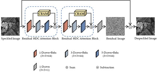
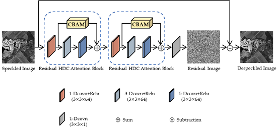
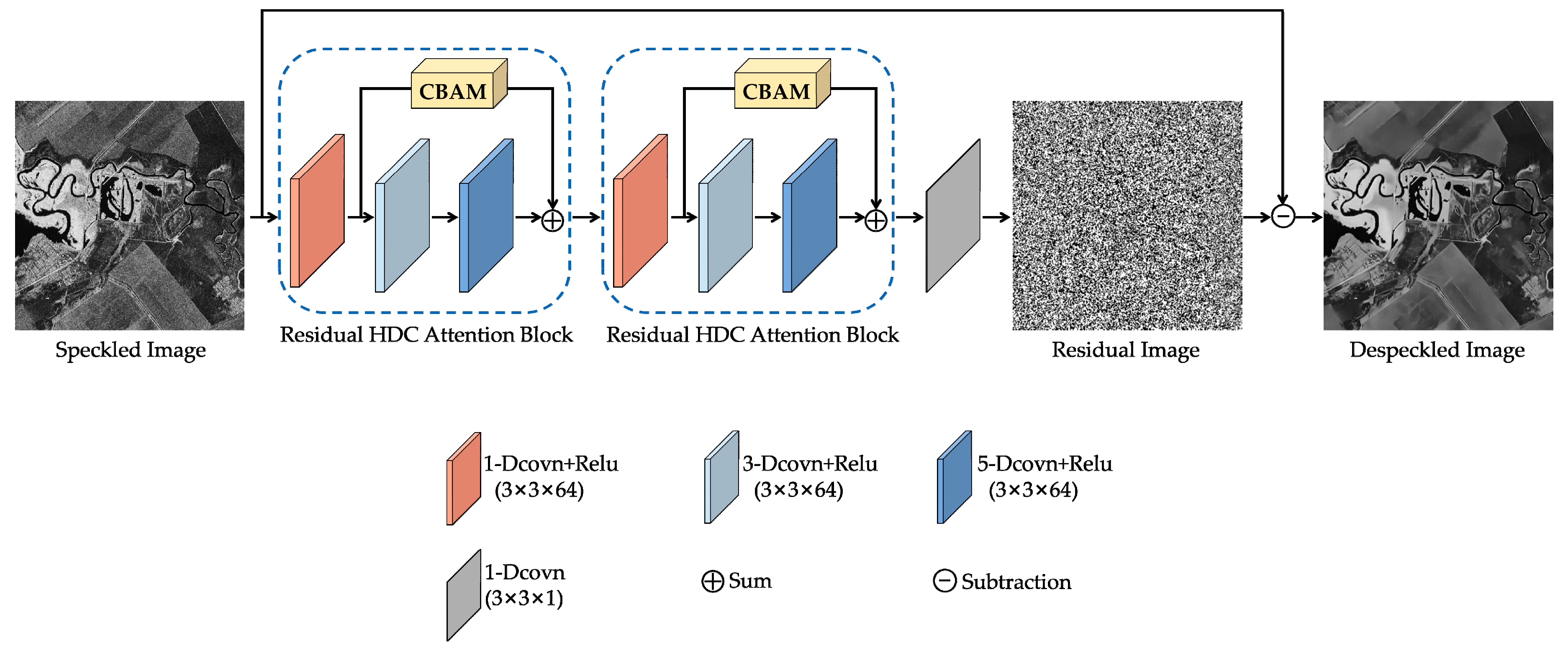
In this section, we present the hybrid dilated residual attention network for SAR image despeckling, i.e., HDRANet, which combines a hybrid dilated convolutional framework HDC with an effective attention module CBAM through skip connection. The proposed HDRANet contains two residual HDC attention blocks and a dilated convolutional layer, as illustrated in Figure 1. With the residual learning strategy, the proposed HDRANet tries to learn the mapping from the speckled image to the estimated pure speckle noise, and then subtracts the pure speckle noise from the speckled image to get the despeckled image. The details of the algorithm are described in the following.

3.1. Hybrid Dilated Convolution

The context information can effectively facilitate the restoration of degraded regions in image denoising. In the CNN model, more contextual information is usually captured by enlarging the receptive field, which is mainly realized via increasing the filter size or stacking convolutional layers. However, these operations will undoubtedly raise the number of parameters and complexity of the model. Recently, the dilated convolution has become popular, as it can effectively enlarge the receptive field while maintaining the filter size and network depth unchanged compared with conventional convolutions.

Figure 2 shows the receptive field size of dilated convolution by different dilate rate. Suppose the kernel size of convolution filters is 3 × 3, in standard convolution, the receptive field size of i-th layer is $(2i+1)\times (2i+1)$, while in dilated convolution, the receptive field grows exponentially in $(2^{i+1}-1)\times (2^{i+1}-1)$ without parameter increase, where $i=1,\dots ,n-1,n$.

However, when a feature map has higher-frequency content than the sampling rate of the dilated convolution, the use of dilated convolution can cause gridding artifacts [40]. Such gridding artifacts may cause the inconsistency of local information and the uncorrelation of information across large distances. To solve this issue, the hybrid dilated convolution (HDC) was proposed in [41].

Assume N convolutional layers with kernel size K × K that dilation rates as $[r_1,\dots ,r_i,\dots ,r_n]$, the HDC aims to let the final size of receptive field fully cover a square region without any holes or missing edges. The maximum distance between two nonzero values $M_i$ is defined as

$$M_i=\max [M_{i+1}-2r_i,M_{i+1}-2(M_{i+1}-r_i),r_i],$$

(4)

where the design goal is to let $M_2\le K$ with $M_n=r_n$. In the proposed HDRANet model, for kernel size 3 × 3, r = [1, 3, 5] pattern works as $M_2=3$, as shown in Figure 3. Clearly, the dilate convolution with different dilate rate extracts features at different scale, which can acquire different levels of context information from local to global. The advantage of HDC is that it can effectively expand the receptive field of CNN to integrate global information of image without causing gridding artifacts. Besides, HDC can be naturally used in CNN without adding extra modules.

3.2. Convolutional Block Attention Module

Recent studies show the effectiveness and significance of attention in enhancing performance of CNN [34,35,36,37,38,39]. Attention tells where to focus and improves the representation of interests, which further improves the expression ability of key features extracted by CNN. Among numerous attention modules, CBAM [37], a lightweight and general module that can be easily integrated into any CNN architecture with negligible overheads, showed efficacy in computer vision problems. Hence, CBAM is introduced into our network to boost the representation power of the features.

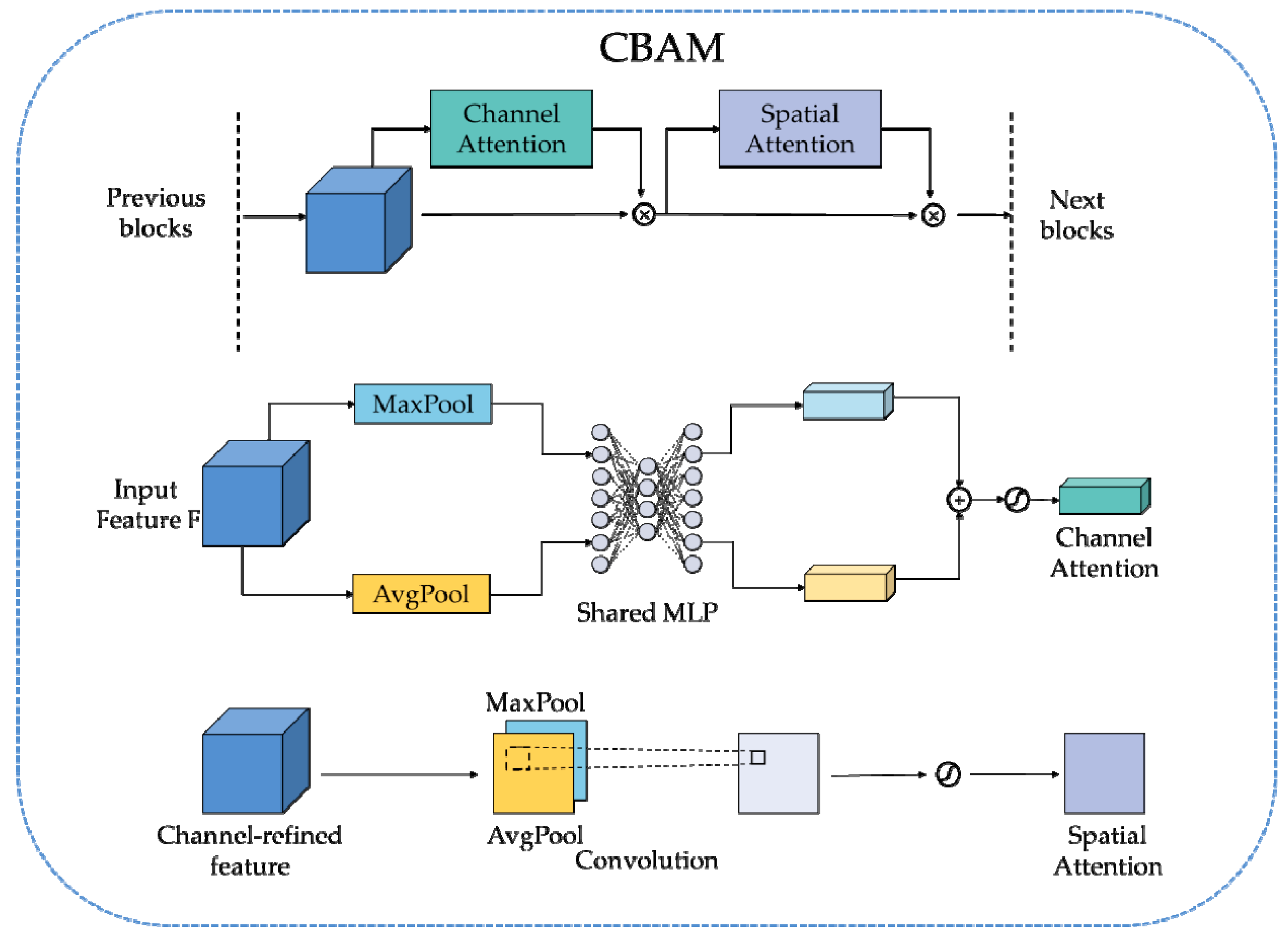
CBAM refine convolutional features by sequentially applying channel and spatial attention modules, as illustrated in Figure 4. Given an input image, the channel attention module concentrates on ‘what’ is meaningful, while the spatial attention module concentrates on ‘where’ is informative, which is a supplement to the channel attention module [37]. In the channel attention module, both average-pooling and max-pooling are performed in the spatial dimension squeezing process, and the average-pooled features and max-pooled features are then forwarded to a multi-layer perceptron (MLP) with one hidden layer whose size is reduced by dividing a reduction ratio to produce the channel attention map. For the spatial attention module, the average and max pooling are applied in the channel axis and concatenate them to generate a spatial attention map by using one 7 × 7 convolution. The channel attention map and spatial attention map are sequentially multiplied to the input feature map for adaptive feature refinement.

3.3. Residual Learning

To address the performance degradation problem that is the accuracy begins to degrade with the network depth increasing, He et al. [42] proposed residual learning by assuming that the residual mapping is much easier to be learned than the original mapping. With the strategy of residual learning, the CNN model even with extremely deep depth can be easily trained and improved performance, which has been achieved in many computer vision tasks.

There are multiple implementations for residual learning. Using a skip connection is a common approach to implement residual learning, which is originally proposed in ResNet [42]. In another implementation, transforming the label data into the difference between the input data and clean data, which has been used in DnCNN [23] for image denoising.

Inspired by those implementations, the proposed HDRANet adopts the residual learning by using a combination of skip connection and transforming label data. The residual HDC attention block employs skip connection to connect the first layer refined by CBAM to the last layer. The skip connection, which passes the feature information of a certain layer to its rear layer, can not only maintain the image details but also alleviate the gradient vanishing problem.

Given $N_u$ training image pairs ${\left\{x_i,y_i\right\}}_{i=1}^{N_u}$, where $x_i$ and $y_i$ denote the clean image and the speckled image respectively. Owing to residual learning formulation employed, residual images as labels are the difference between the input speckled image and the clean image. Therefore, the loss function using the mean squared error (MSE) is defined as follows:

$$loss(\Theta )=\frac{1}{2N_u}{{\displaystyle \sum _{i=1}^{N_u}\Vert R\left(y_i,\Theta \right)-\left(y_i-x_i\right)\Vert }}^2,$$

(5)

where $\Theta$ represents the trainable parameters in HDRANet.

4. Experiment Results

4.1. Experimental Setting

4.1.1. Training Data

In the experiment, we took the UC Merced land-use dataset [43] as training dataset for simulating SAR image despeckling. This dataset contained 21 different scene classes and each class had 100 images with a size of 256 × 256. To train the proposed HDRANet, we chose 50 images from per class in total 1050 images and set a patch size as 64 × 64 and crop 177450 patches with stride equal to 15. In addition, we injected speckle in amplitude format on those optical images, where three different noise levels with the number of looks L = 1, 2, 4 were set to add speckle noise respectively.

4.1.2. Parameter Setting and Network Training

We used the Adam [44] solver to optimize the proposed HDRANet with momentum ${\beta }_1=0.9$, momentum ${\beta }_2=0.999$, $\epsilon ={10}^{-8}$, and decay = 0. We trained our model 50 epochs with a mini-batch size of 128. The learning rate was initially set as 0.001 and decreased after every 10 epochs by multiplying 0.2. The HDRANet was implemented using Pytorch framework in Ubuntu 16.04.1 with NVIDIA GeForce GTX-1080 Ti (12G) GPU. It took about 3 hours to train HDRANet. The network parameters are listed in

Table 1. The network parameters.

Name	Parameters
1-Dcovn+Relu	3 × 3 × 64, dilate = 1, padding = 1, stride = 1
3-Dcovn+Relu	3 × 3 × 64, dilate = 3, padding = 3, stride = 1
5-Dcovn+Relu	3 × 3 × 64, dilate = 5, padding = 5, stride = 1
CBAM	Channel attention, the reduction ratio of MLP: r = 16 Spatial attention, the filter size of convolution: 7 × 7 × 1
1-Dcovn	3 × 3 × 1, dilate = 1, padding = 1, stride = 1

.

4.2. Quantitative Evaluations

In the synthetic image experiments, we used the peak signal-to-noise ratio (PSNR) and structural similarity (SSIM) as metrics to evaluate the despeckling performances. The PSNR is defined as follows:

$$PSNR(f,g)=10lo{g}_{10}\left(\frac{{255}^2}{MSE(f,g)}\right),$$

(6)

$$MSE(f,g)=\frac{1}{HW}{\displaystyle \sum _{i=1}^H{\displaystyle \sum _{j=1}^W{\Vert f(i,j)-g(i,j)\Vert }^2}},$$

(7)

where $f$ and $g$ represent the original image and the despeckled image, respectively. H is the height of the image and W is the weight of the image. $f\left(i,j\right)$ and $g\left(i,j\right)$ are the pixel value at the position of the original image and the despeckled image respectively. The higher PSNR values, the better speckle noise reduction performances. The SSIM is given as follows:

$$SSIM(f,g)=\frac{\left(2{\mu }_f{\mu }_g+c_1\right)\left(2co{v}_{fg}+c_2\right)}{\left({\mu }_f{}^2+{\mu }_g{}^2+c_1\right)\left({\sigma }_f{}^2+{\sigma }_g{}^2+c_2\right)}.$$

(8)

Here, ${\mu }_f$ and ${\mu }_g$ present the mean of $f$ and $g$, respectively. $co{v}_{fg}$ is the covariance of $f$, $g$. ${\sigma }_f{}^2$ is the variance of $f$ and ${\sigma }_g{}^2$ is the variance of $g$. $c_1$ and $c_2$ are two variables to stabilize the division. The value of SSIM is between [0,1], and the value closer to 1 indicates better speckle noise reduction performances. The equivalent number of look (ENL) is one of the widely used quantitative evaluation index for the real SAR image despeckling, which evaluates the smoothness of a homogeneous regions in the image after despeckling. The ENL is defined by:

$$ENL=\frac{{\mu }^2}{{\sigma }^2},$$

(9)

where ${\mu }_{}$ and $\sigma$ are the image mean and variance. The larger ENL demonstrate that the homogeneous region is smoother and the speckle noise removal performances are more excellent.

4.3. Results on Synthetic Images

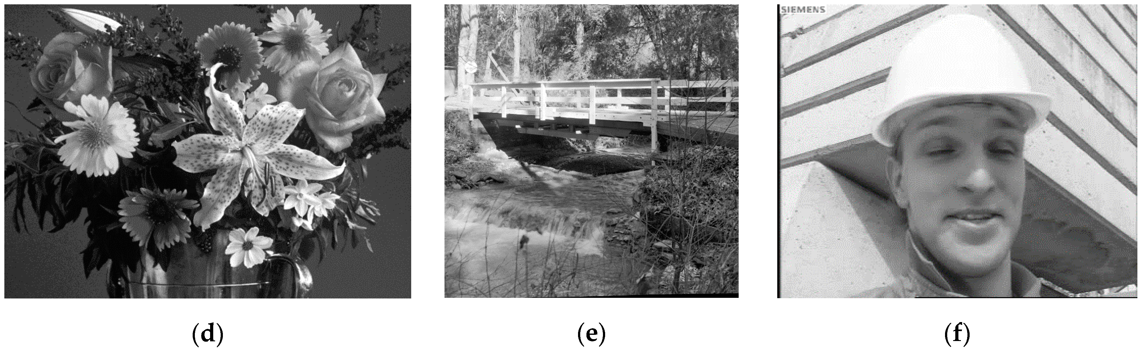
As shown in Figure 5, we selected six gray images as test images for synthetic image experiments. To verify the despeckling effectiveness of the proposed HDRANet, three different speckle noise level of L = 1, 2, and 4 were set up for the six synthetic images. To evaluate the speckle noise reduction performances on synthetic images, we compared our HDRANet with several representative despeckling methods, including one spatial domain filter method (Lee [2]), two nonlocal means methods (PPB [13] and SAR-BM3D [14]) and one CNN-based method (SAR-DRN [28]). In comparison methods, all the parameters were set as suggested in their corresponding papers.

As shown in

Table 2. Quantitative results on synthetic images (L = 1). The best performance is marked in bold.

Image	Index	Noisy	Lee	PPB	SAR-BM3D	SAR-DRN	HDRANet
Airplane	PSNR	11.17	17.23	19.57	21.32	23.21	23.36
	SSIM	0.151	0.312	0.550	0.679	0.702	0.701
Ship	PSNR	12.33	20.51	21.71	23.36	22.68	24.31
	SSIM	0.161	0.389	0.536	0.637	0.654	0.655
Couple	PSNR	12.72	20.92	21.34	23.04	23.69	25.18
	SSIM	0.177	0.412	0.512	0.638	0.666	0.674
Bridge	PSNR	13.27	20.15	19.80	21.42	22.64	22.83
	SSIM	0.261	0.500	0.400	0.553	0.586	0.586
Flowers	PSNR	15.12	22.23	21.44	23.35	25.02	25.14
	SSIM	0.303	0.593	0.609	0.725	0.754	0.754
Foreman	PSNR	11.45	17.25	19.70	21.19	25.32	26.16
	SSIM	0.101	0.312	0.644	0.747	0.784	0.780
Average	PSNR	12.68	19.72	20.59	22.28	23.76	24.50
	SSIM	0.192	0.420	0.542	0.663	0.691	0.692

,

Table 3. Quantitative results on synthetic images (L = 2). The best performance is marked in bold.

Image	Index	Noisy	Lee	PPB	SAR-BM3D	SAR-DRN	HDRANet
Airplane	PSNR	13.53	20.33	21.67	23.87	24.61	24.96
	SSIM	0.216	0.413	0.638	0.747	0.758	0.760
Ship	PSNR	14.69	23.01	23.97	25.53	24.63	27.17
	SSIM	0.233	0.486	0.613	0.698	0.708	0.709
Couple	PSNR	15.21	23.36	23.65	25.67	26.01	26.19
	SSIM	0.258	0.521	0.606	0.725	0.740	0.738
Bridge	PSNR	15.79	22.20	21.60	23.32	24.06	23.91
	SSIM	0.379	0.591	0.509	0.656	0.671	0.675
Flowers	PSNR	17.69	24.34	24.03	25.47	26.28	26.88
	SSIM	0.418	0.691	0.717	0.797	0.812	0.815
Foreman	PSNR	14.02	20.48	22.56	24.41	27.24	28.30
	SSIM	0.158	0.436	0.730	0.812	0.824	0.826
Average	PSNR	15.16	22.29	22.91	24.71	25.47	26.24
	SSIM	0.277	0.523	0.636	0.739	0.752	0.754

and

Table 4. Quantitative results on synthetic images (L = 4). The best performance is marked in bold.

Image	Index	Noisy	Lee	PPB	SAR-BM3D	SAR-DRN	HDRANet
Airplane	PSNR	15.90	22.84	24.09	25.92	26.50	26.51
	SSIM	0.286	0.505	0.718	0.800	0.809	0.809
Ship	PSNR	17.30	25.05	26.23	27.67	28.36	28.57
	SSIM	0.320	0.581	0.682	0.753	0.762	0.760
Couple	PSNR	17.86	25.41	25.99	27.80	27.37	27.91
	SSIM	0.353	0.618	0.696	0.784	0.793	0.795
Bridge	PSNR	18.48	23.82	23.50	25.13	24.43	25.81
	SSIM	0.509	0.666	0.618	0.748	0.747	0.755
Flowers	PSNR	20.40	25.99	26.30	27.39	27.52	27.49
	SSIM	0.535	0.763	0.795	0.847	0.854	0.855
Foreman	PSNR	16.65	23.52	25.98	27.47	29.38	29.52
	SSIM	0.233	0.551	0.807	0.855	0.857	0.855
Average	PSNR	17.77	24.44	25.35	26.90	27.26	27.64
	SSIM	0.373	0.614	0.719	0.798	0.804	0.805

, the proposed HDRANet model obtained almost the best PSNR and SSIM results in the three noise levels. When L = 1, 2, and 4, the proposed method outperformed Lee, PPB, SAR-BM3D, and SAR-DRN by about 4.78 dB/3.95 dB/3.2 dB, 3.91 dB/3.33 dB/2.29 dB, 2.22 dB/1.53 dB/0.74 dB, and 0.74 dB/0.77 dB/0.38 dB for the average PSNR of six test images, respectively. As highlighted in Table 2, Table 3 and Table 4 (the best performance is marked in bold), the proposed HDRANet outperformed other algorithms above also in terms of average SSIM, providing more accurate preservation of the image structural information. Clearly, HDRANet achieved the best performance over other despeckling methods in terms of the quantitative assessments.

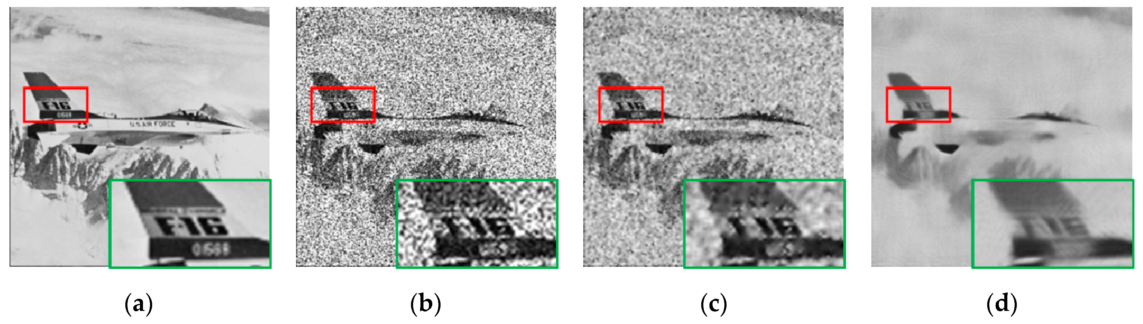
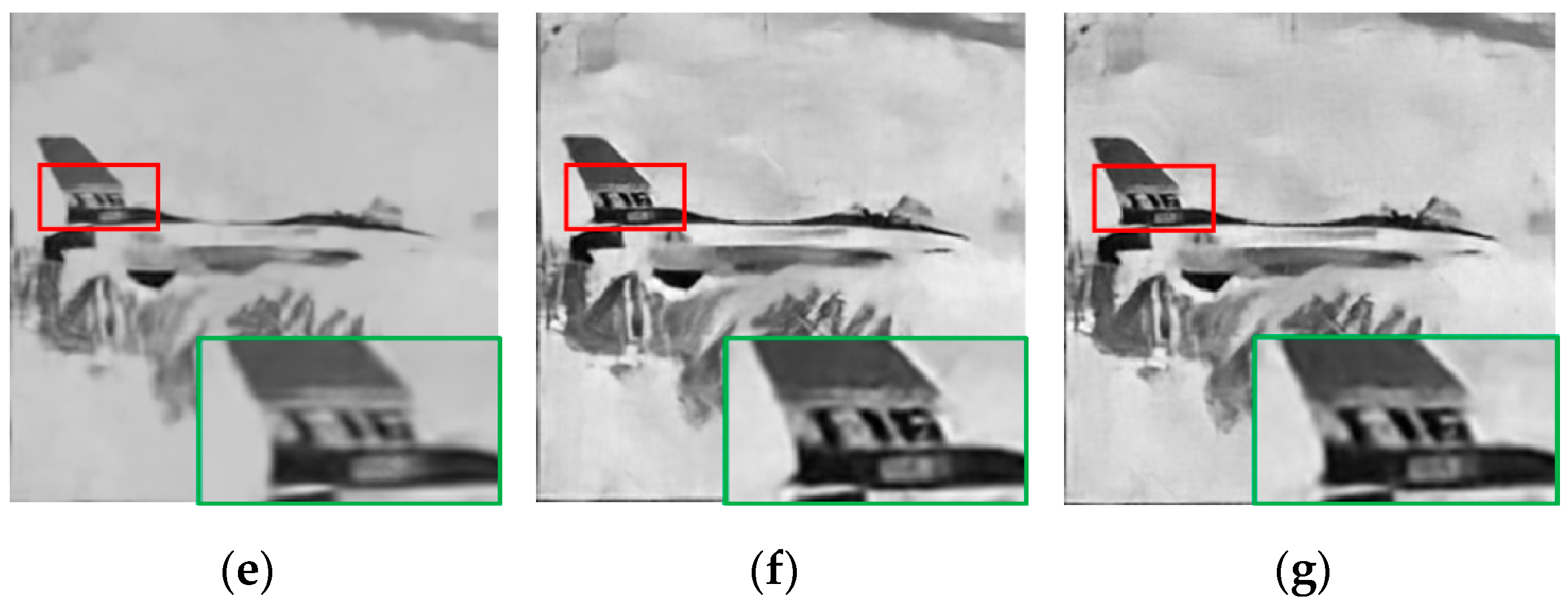
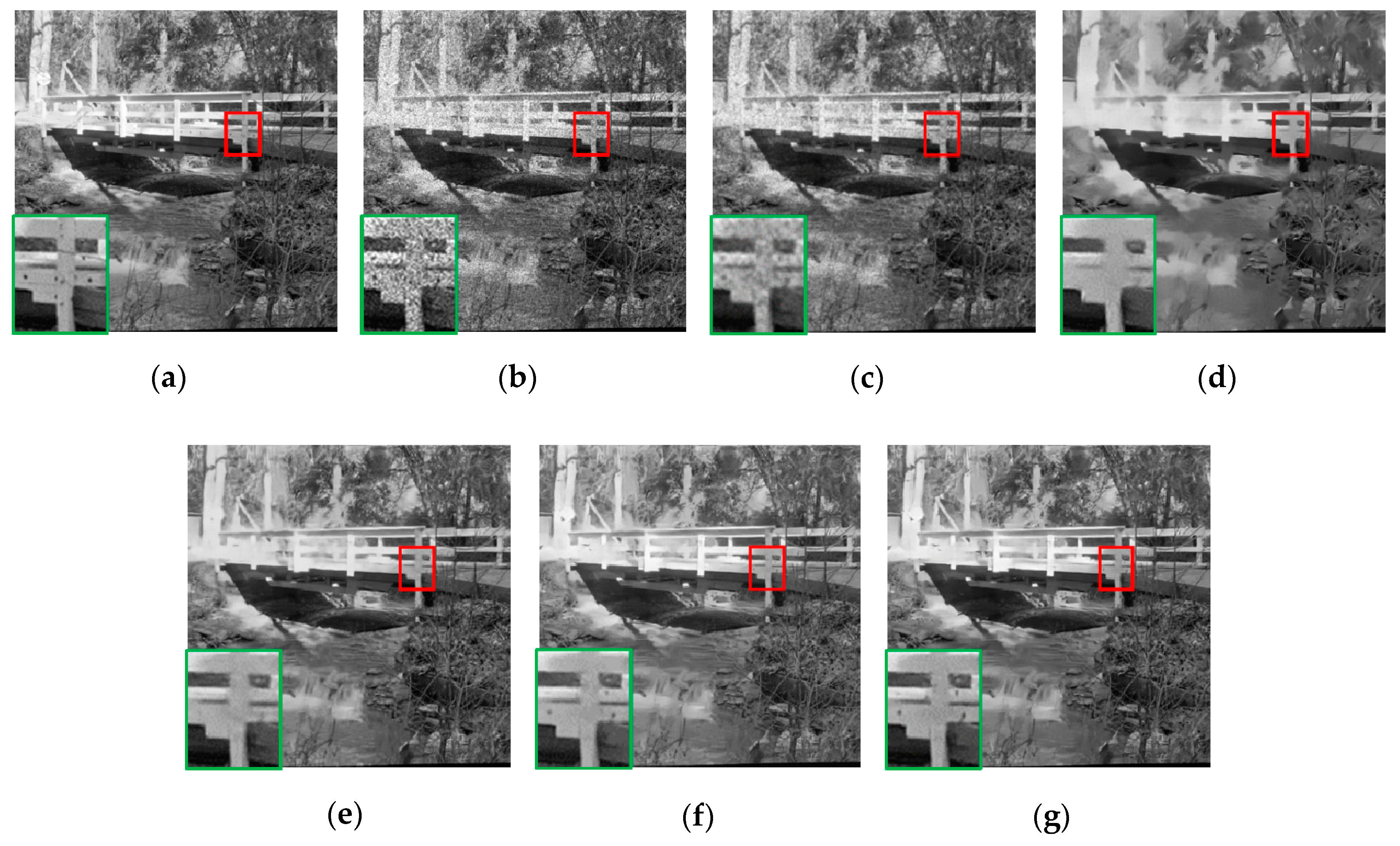
Figure 6, Figure 7 and Figure 8 correspondingly represent the despeckled images for the airplane, flowers, and bridge image degraded by the noise level L = 1, 2, 4, respectively. Obviously, the results of Lee still suffered from the residual noise. PPB worked well in speckle reduction, but simultaneously generated numerous unexpected texture distortions, especially around the edges of images. SAR-BM3D performed better than PPB, which effectively reduced speckle and created fewer texture distortions. However, SAR-BM3D tended to produce over-smooth edges and textures, as it mainly focused on some complex geometric features. SAR-DRN removed the speckle well and preserved local details. It could be clearly seen that HDRANet could remove the speckle satisfactorily and preserve sharp edges and fine details, showing the best speckle-reduction and local detail preservation ability. Compared with the other algorithms above, the proposed HDRANet method showed much more advantageous performance in both quantitative and visual assessments, especially for strong speckle noise.

4.4. Results on Real SAR Images

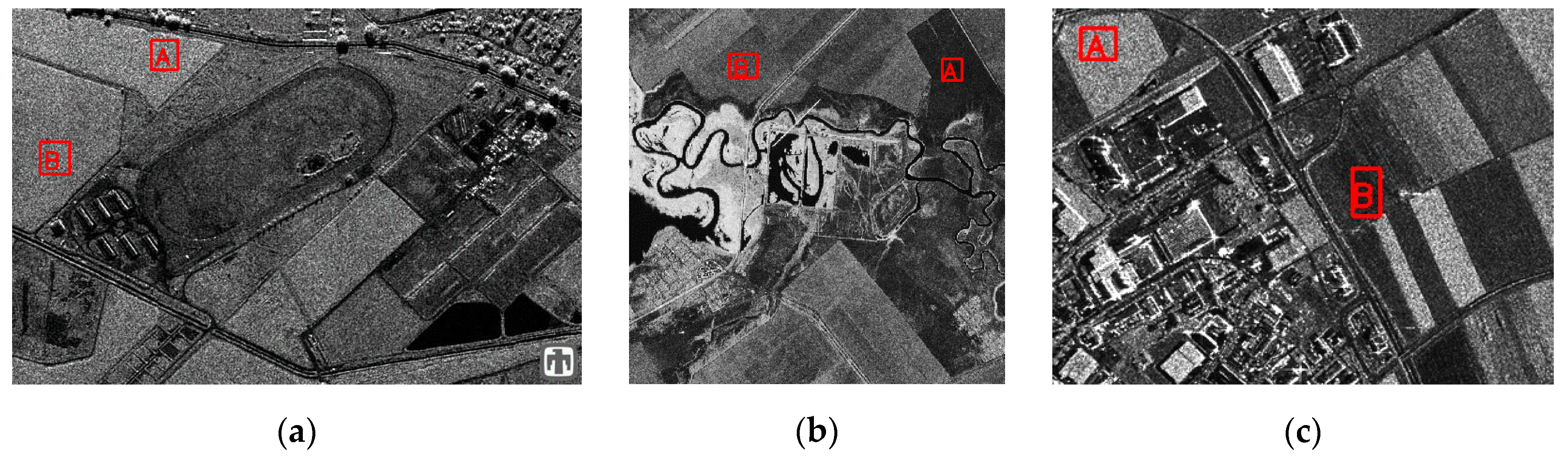
In this part, three real SAR images, which were all four-look data were chosen to evaluate the proposed method. Figure 9a is a Ku-band 1-m resolution SAR image over a horse track near Albuquerque, NM, Figure 9b shows a 10-m resolution TerraSAR-X image of scenes from the west of Volgograd, Russia, and Figure 9c shows a 1-m resolution TerraSAR-X image of the landscapes in Noerdlingen, Germany [45]. For the real SAR images, we also compared HDRANet with the four methods mentioned above.

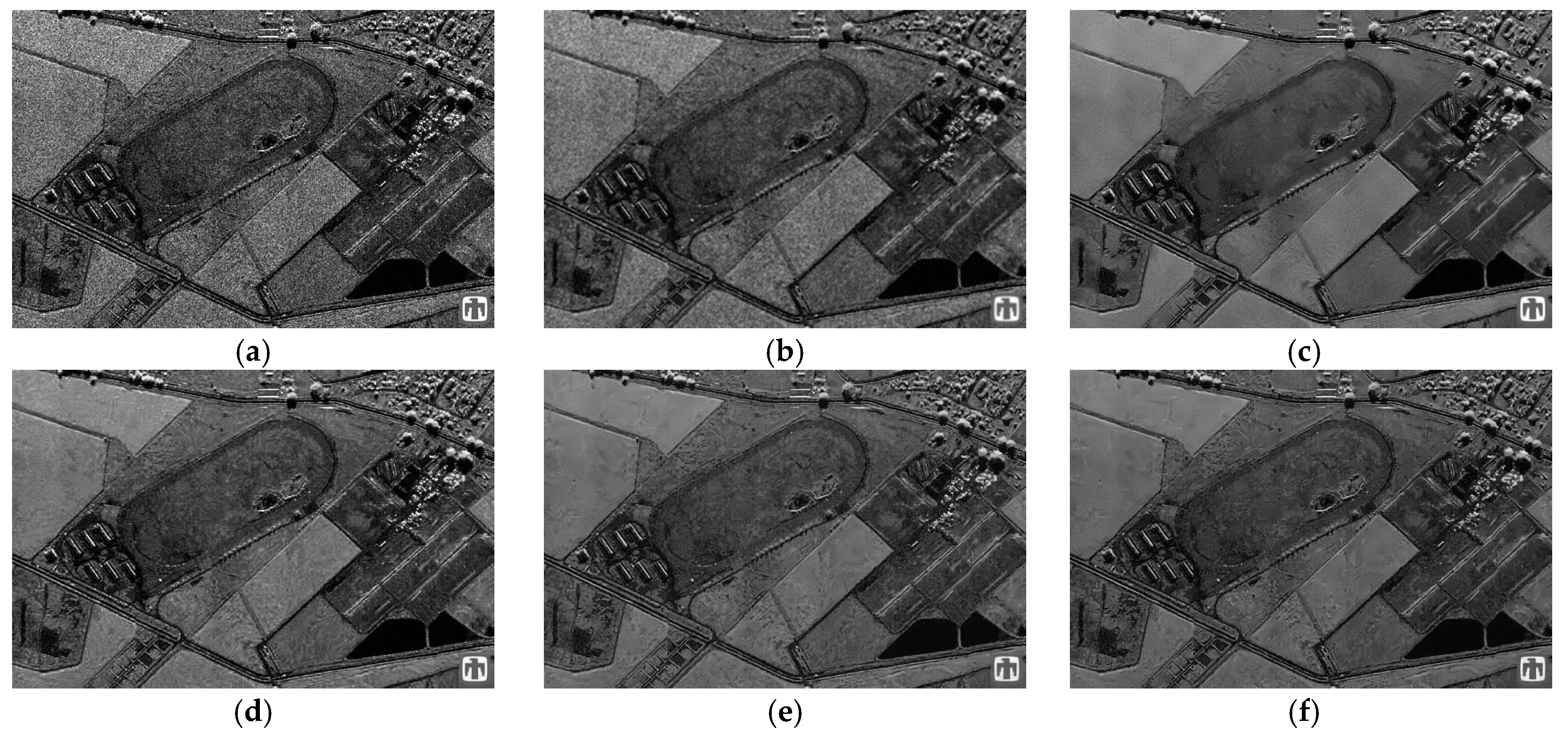
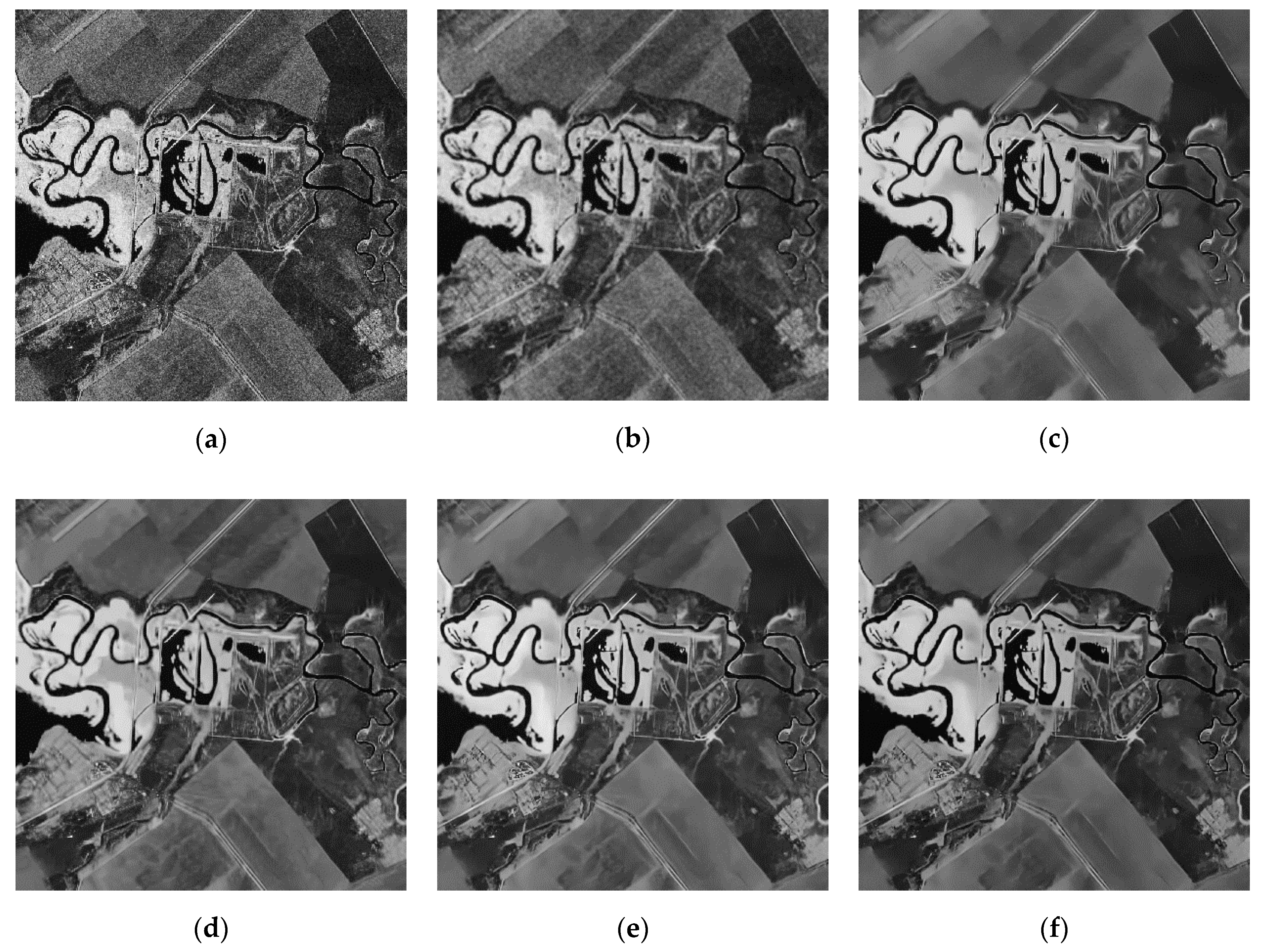
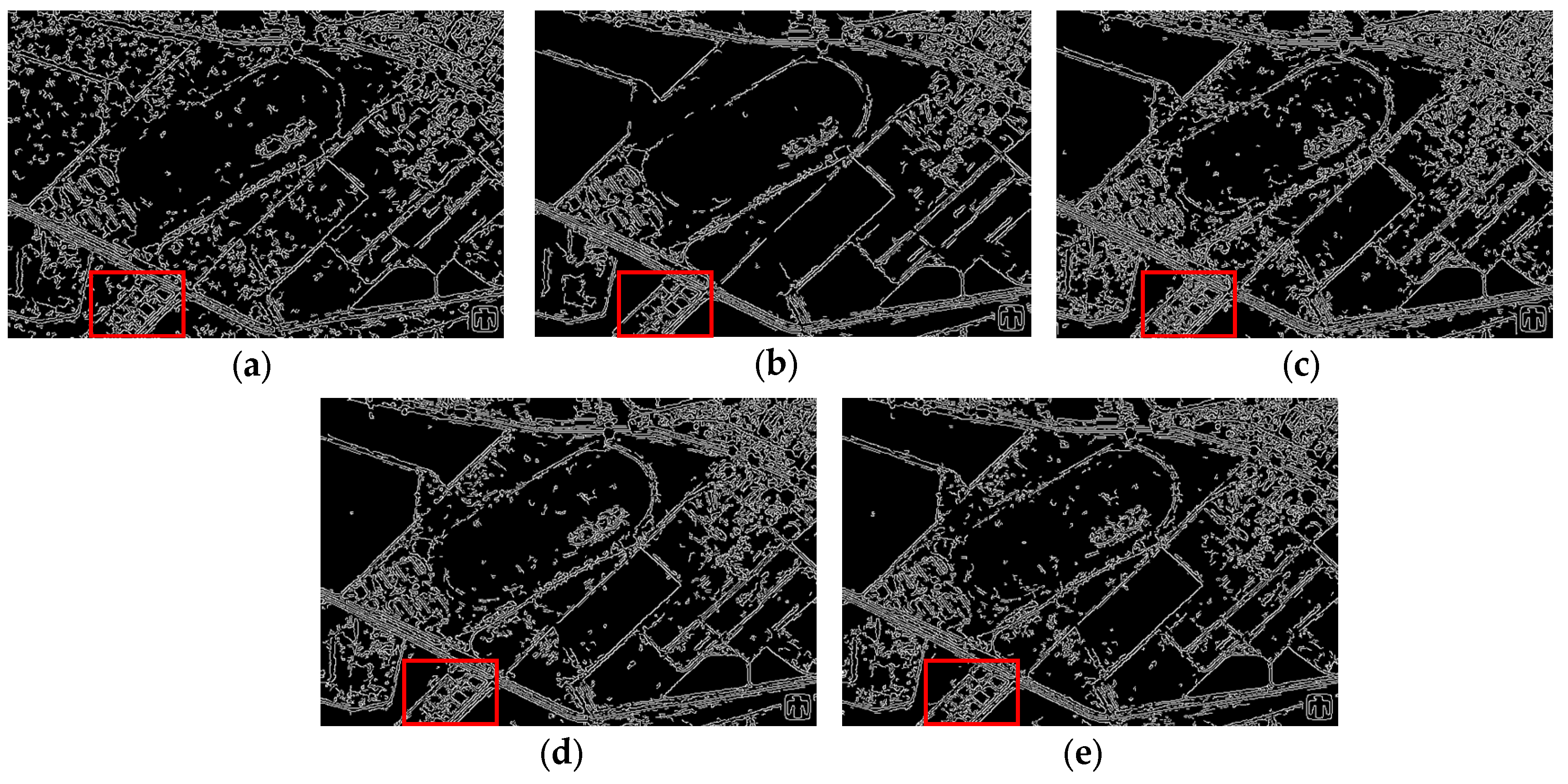
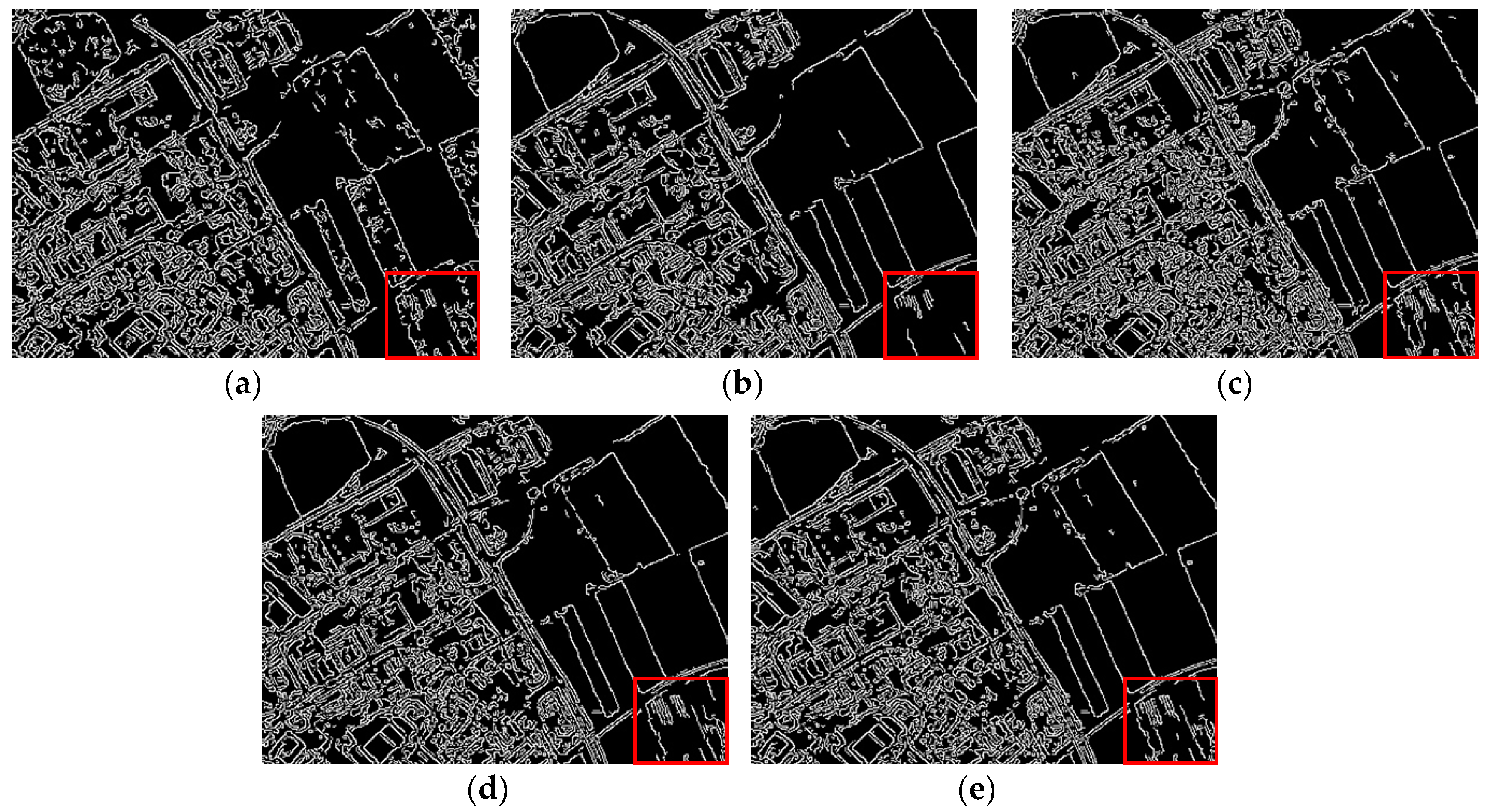
From Figure 10, Figure 11 and Figure 12, it was obvious that the results of Lee and SAR-BM3D still contained a lot of residual speckle noise, while the results of PPB, SAR-DRN, and the proposed HDRANet performed well in speckle suppression. PPB revealed good speckle-reduction ability, but it resulted in an over-smoothing phenomenon. In homogeneous regions, the proposed HDRANet outperformed SAR-DRN in speckle reduction. Visually, HDRANet also obtained the best performance in both speckle removal and sharp edges and fine details preservation, which was superior to the other four methods. For the real SAR images, the corresponding noise-free images were not available. In order to provide some measure of objective for comparison of results, we used ENL and the corresponding edge images of the despeckled and images by using a Canny edge detector to measure the speckle-reduction and edge-preserving ability, respectively. Two homogeneous areas, namely, region A and B were selected in each original SAR image (Figure 9a–c). The selected regions composed of 28 pixels × 31 pixels and 31 pixels × 34 pixels for the horsetrack, 21 pixels × 23 pixels and 22 pixels × 38 pixels for Volgograd, and 28 pixels × 25 pixels and 35 pixels × 34 pixels for Noerdlingen.

From

Table 5. Equivalent number of look (ENL) results for three real SAR images. The best performance is marked in bold.

Image	Area	Noisy	Lee	PPB	SAR-BM3D	SAR-DRN	HDRANet
Horsetrack	A	18.86	95.48	1163.52	408.50	1396.85	1415.08
	B	15.69	95.33	940.78	338.51	807.16	944.62
Volgograd	A	24.58	80.61	336.19	197.16	389.74	508.59
	B	19.38	121.26	1276.60	751.99	1500.98	1659.79
Noerdlingen	A	18.52	107.32	2143.67	505.04	1735.32	2193.07
	B	12.21	37.09	75.49	43.86	60.66	76.50

and Figure 13, Figure 14 and Figure 15(the best performance is marked in bold), it could be clearly seen that HDRANet had a much better speckle-reduction and edge-preserving ability than the other methods, which was accordant with the visual observation.

5. Ablation Study

In this section, we empirically showed that our design choice was valid. For this ablation study, we used the Set12 dataset [23] as the test dataset. We first verified the effectiveness of convolutional block attention module (CBAM) and then analyzed the reason why we chose two residual HDC attention block. We explained the details of each experiment below.

5.1. Convolutional Block Attention Module

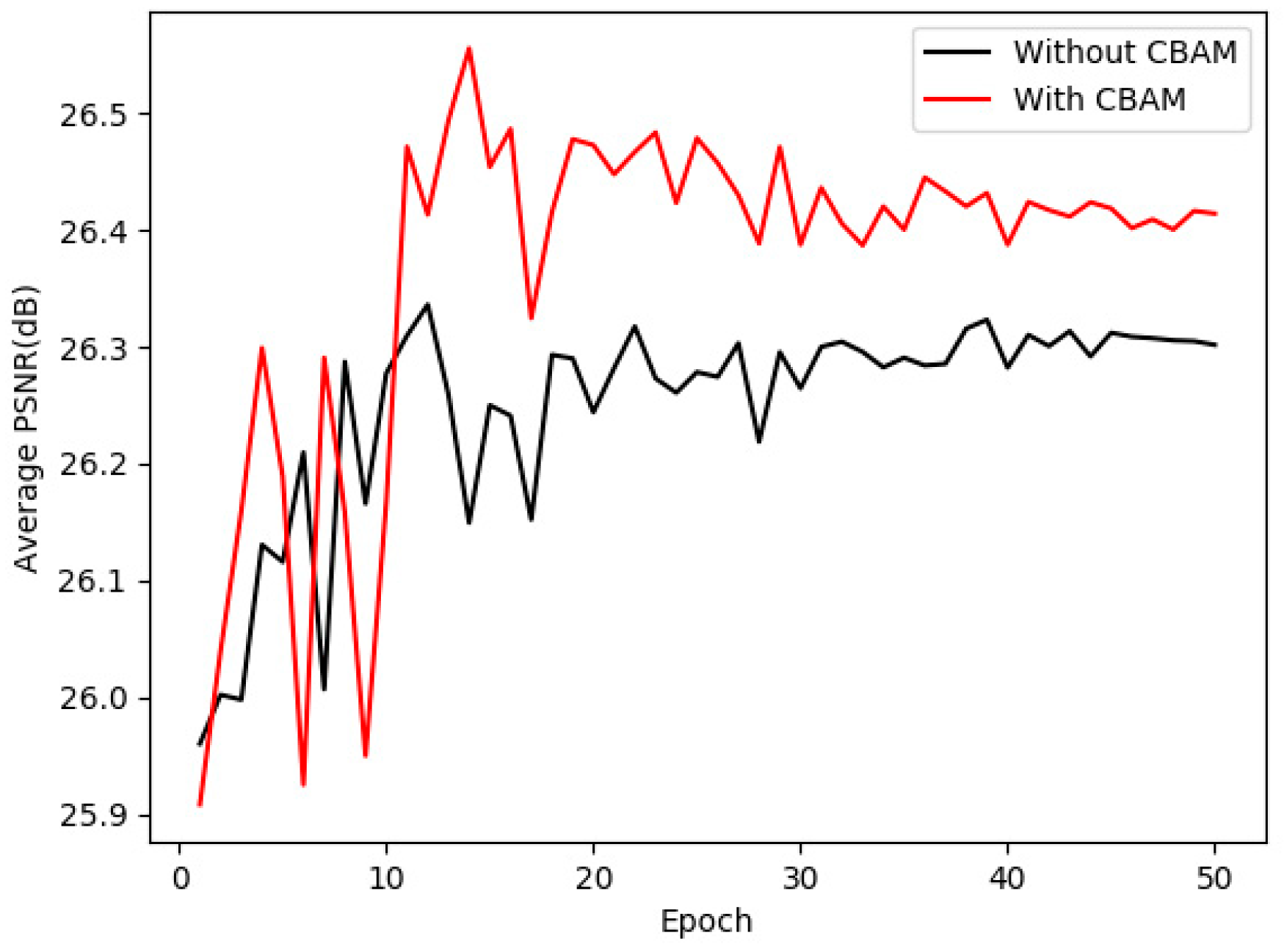
As described in Section III, the proposed method HDRANet employs CBAM, which can increase the representation power of CNN by focusing on important features and suppressing unnecessary ones. To verify the effectiveness of CBAM, we implemented two sets of experiments in the same environment with the speckle noise level of L = 4. As that shown in Figure 16, the model with CBAM was up from about 0.1 dB in the average PSNR of the test dataset compared with the model without CBAM. Therefore, CBAM could enhance the despeckling performance of CNN networks and help to construct a final despeckled image.

5.2. Residual HDC Attention Block

Figure 17 shows the performance of the different blocks on the test dataset, with the average PSNR results evaluated at the end of each training epoch. As can be observed in the figure, curves show that the two blocks obtained the best performance after 10 epochs. For the reason, we considered that the one-block model had insufficient representational capacity because of the shallow architecture, while the three-block and four-block models were complex resulting to overfitting. To get the superior performance while maintaining network lightweight, we used two residual HDC attention blocks in the proposed model.

6. Conclusions

In this paper, we proposed a hybrid dilated residual attention network to remove the speckle noise in SAR, which applies a residual learning strategy to separate speckle noise from noisy observation. The proposed HDRANet integrates hybrid dilated convolution (HDC) and the convolutional block attention module (CBAM) with a residual structure. HDC effectively enlarges the receptive field of the network to aggregate global information, while CBAM enhances representation power and performance of the network. In both synthetic and real SAR image despeckling experiments, the proposed method achieved superior despeckling performance over the state-of-the-art methods in terms of both quantitative and qualitative assessments. In the future work, we planned to extend our model to the generative adversarial network architecture and use adversarial training to further improve the despeckling performance. Furthermore, we will consider addressing the SAR image blind despeckling, which aims to remove unknown noise-level speckle noise from SAR image.

References

- Argenti, F.; Lapini, A.; Bianchi, T.; Alparone, L. A tutorial on speckle reduction in synthetic aperture radar images. IEEE Geosci. Remote Sens. Mag. 2013, 1, 6–35. [Google Scholar] [CrossRef] [Green Version]
- Lee, J.-S. Digital image enhancement and noise filtering by use of local statistics. IEEE Trans. Pattern Anal. Mach. Intell. 1980, PAMI-2, 165–168. [Google Scholar] [CrossRef] [PubMed] [Green Version]
- Kuan, D.T.; Sawchuk, A.A.; Strand, T.C.; Chavel, P. Adaptive noise smoothing filter for images with signal-dependent noise. IEEE Trans. Pattern Anal. Mach. Intell. 1985, PAMI-7, 165–177. [Google Scholar] [CrossRef] [PubMed]
- Frost, V.S.; Stiles, J.A.; Shanmugan, K.S.; Holtzman, J.C. A model for radar images and its application to adaptive digital filtering of multiplicative noise. IEEE Trans. Pattern Anal. Mach. Intell. 1982, PAMI-4, 157–166. [Google Scholar] [CrossRef]
- Lopes, A.; Nezry, E.; Touzi, R.; Laur, H. Maximum a posteriori speckle filtering and first order texture models in SAR images. In Proceedings of the 10th Annual International Symposium on Geoscience and Remote Sensing, College Park, MD, USA, 20–24 May 1990; pp. 2409–2412. [Google Scholar]
- Chang, S.G.; Yu, B.; Vetterli, M. Spatially adaptive wavelet thresholding with context modeling for image denoising. IEEE Trans. Image Process. 2000, 9, 1522–1531. [Google Scholar] [CrossRef] [Green Version]
- Kalaiyarasi, M.; Saravanan, S.; Perumal, B. A survey on: De-speckling methods Of SAR image. In Proceedings of the 2016 International Conference on Control, Instrumentation, Communication and Computational Technologies (ICCICCT), Kumaracoil, India, 16–17 December 2016; pp. 54–63. [Google Scholar]
- Gleich, D. Markov Random Field Models for Non-Quadratic Regularization of Complex SAR Images. IEEE J. Sel. Top. Appl. Earth Obs. Remote Sens. 2012, 5, 952–961. [Google Scholar] [CrossRef]
- Mahdianpari, M.; Motagh, M.; Akbari, V.; Mohammadimanesh, F.; Salehi, B. A Gaussian random field model for de-speckling of multi-polarized Synthetic Aperture Radar data. Adv. Space Res. 2019, 64, 64–78. [Google Scholar] [CrossRef]
- Rudin, L.; Lions, P.-L.; Osher, S. Multiplicative denoising and deblurring: Theory and algorithms. In Geometric Level Set Methods in Imaging, Vision, and Graphics; Springer: Berlin, Germany, 2003; pp. 103–119. [Google Scholar]
- Aubert, G.; Aujol, J.-F. A variational approach to removing multiplicative noise. SIAM J. Appl. Math. 2008, 68, 925–946. [Google Scholar] [CrossRef]
- Buades, A.; Coll, B.; Morel, J.-M. A non-local algorithm for image denoising. In Proceedings of the 2005 IEEE Computer Society Conference on Computer Vision and Pattern Recognition (CVPR’05), San Diego, CA, USA, 20–25 June 2005; pp. 60–65. [Google Scholar]
- Deledalle, C.-A.; Denis, L.; Tupin, F. Iterative weighted maximum likelihood denoising with probabilistic patch-based weights. IEEE Trans. Image Process. 2009, 18, 2661–2672. [Google Scholar] [CrossRef] [Green Version]
- Parrilli, S.; Poderico, M.; Angelino, C.V.; Verdoliva, L. A nonlocal SAR image denoising algorithm based on LLMMSE wavelet shrinkage. IEEE Trans. Geosci. Remote Sens. 2011, 50, 606–616. [Google Scholar] [CrossRef]
- Zhang, H.; Li, Y.; Jiang, Y.; Wang, P.; Shen, Q.; Shen, C. Hyperspectral Classification Based on Lightweight 3-D-CNN With Transfer Learning. IEEE Trans. Geosci. Remote Sens. 2019, 57, 5813–5828. [Google Scholar] [CrossRef] [Green Version]
- Fang, B.; Li, Y.; Zhang, H.; Chan, J.C.-W. Hyperspectral Images Classification Based on Dense Convolutional Networks with Spectral-Wise Attention Mechanism. Remote Sens. 2019, 11, 159. [Google Scholar] [CrossRef] [Green Version]
- Zhang, H.; Li, Y.; Zhang, Y.; Shen, Q. Spectral-spatial classification of hyperspectral imagery using a dual-channel convolutional neural network. Remote Sens. Lett. 2017, 8, 438–447. [Google Scholar] [CrossRef] [Green Version]
- He, K.; Gkioxari, G.; Dollár, P.; Girshick, R. Mask r-cnn. In Proceedings of the 2017 IEEE International Conference on Computer vision, Venice, Italy, 22–29 October 2017; pp. 2961–2969. [Google Scholar]
- Long, J.; Shelhamer, E.; Darrell, T. Fully convolutional networks for semantic segmentation. In Proceedings of the 2015 IEEE Conference on Computer Vision and Pattern Recognition, Boston, MA, USA, 7–12 June 2015; pp. 3431–3440. [Google Scholar]
- Wang, D.; Li, Y.; Ma, L.; Bai, Z.; Chan, J.C.-W. Going Deeper with Dense Connectedly Convolutional Neural Networks for Multispectral Pansharpening. Remote Sens. 2019, 11, 2608. [Google Scholar] [CrossRef] [Green Version]
- Danelljan, M.; Robinson, A.; Khan, F.S.; Felsberg, M. Beyond correlation filters: Learning continuous convolution operators for visual tracking. In Proceedings of the 14th European Conference on Computer Vision, Amsterdam, The Netherlands, 11–14 October 2016; pp. 472–488. [Google Scholar]
- Mao, X.; Shen, C.; Yang, Y.-B. Image restoration using very deep convolutional encoder-decoder networks with symmetric skip connections. In Advances in Neural Information Processing Systems 29: 30th Conference on Neural Information Processing Systems, NIPS 2016; Curran Associates, Inc.: New York, NY, USA, 2017; pp. 2802–2810. [Google Scholar]
- Zhang, K.; Zuo, W.; Chen, Y.; Meng, D.; Zhang, L. Beyond a gaussian denoiser: Residual learning of deep cnn for image denoising. IEEE Trans. Image Process. 2017, 26, 3142–3155. [Google Scholar] [CrossRef] [Green Version]
- Zhang, K.; Zuo, W.; Zhang, L. FFDNet: Toward a fast and flexible solution for CNN-based image denoising. IEEE Trans. Image Process. 2018, 27, 4608–4622. [Google Scholar] [CrossRef] [Green Version]
- Guo, S.; Yan, Z.; Zhang, K.; Zuo, W.; Zhang, L. Toward convolutional blind denoising of real photographs. In Proceedings of the 2019 IEEE Conference on Computer Vision and Pattern Recognition, Los Angeles, CA, USA, 15–21 June 2019; pp. 1712–1722. [Google Scholar]
- Chierchia, G.; Cozzolino, D.; Poggi, G.; Verdoliva, L. SAR image despeckling through convolutional neural networks. In Proceedings of the 2017 IEEE International Geoscience and Remote Sensing Symposium (IGARSS), Fort Worth, TX, USA, 23–28 July 2017; pp. 5438–5441. [Google Scholar]
- Wang, P.; Zhang, H.; Patel, V.M. SAR image despeckling using a convolutional neural network. IEEE Signal. Process. Lett. 2017, 24, 1763–1767. [Google Scholar] [CrossRef] [Green Version]
- Zhang, Q.; Yuan, Q.; Li, J.; Yang, Z.; Ma, X. Learning a dilated residual network for SAR image despeckling. Remote Sens. 2018, 10, 196. [Google Scholar] [CrossRef] [Green Version]
- Mohammadimanesh, F.; Salehi, B.; Mahdianpari, M.; Gill, E.; Molinier, M. A new fully convolutional neural network for semantic segmentation of polarimetric SAR imagery in complex land cover ecosystem. ISPRS J. Photogramm. Remote Sens. 2019, 151, 223–236. [Google Scholar] [CrossRef]
- Moreira, A. Improved multilook techniques applied to SAR and SCANSAR imagery. IEEE Trans. Geosci. Remote Sens. 1991, 29, 529–534. [Google Scholar] [CrossRef]
- Jain, V.; Seung, S. Natural image denoising with convolutional networks. In Advances in Neural Information Processing Systems 21: 22nd Conference on Neural Information Processing Systems 2008, NIPS 2008; Curran Associates, Inc.: New York, NY, USA, 2009; pp. 769–776. [Google Scholar]
- Simonyan, K.; Zisserman, A. Very deep convolutional networks for large-scale image recognition. arXiv 2014, arXiv:1409.1556. [Google Scholar]
- Lattari, F.; Gonzalez Leon, B.; Asaro, F.; Rucci, A.; Prati, C.; Matteucci, M. Deep Learning for SAR Image Despeckling. Remote Sens. 2019, 11, 1532. [Google Scholar] [CrossRef] [Green Version]
- Jaderberg, M.; Simonyan, K.; Zisserman, A. Spatial transformer networks. In Advances in Neural Information Processing Systems 28: 29th Conference on Neural Information Processing Systems 2015, NIPS 2015; Curran Associates, Inc.: New York, NY, USA, 2016; pp. 2017–2025. [Google Scholar]
- Hu, J.; Shen, L.; Sun, G. Squeeze-and-excitation networks. In Proceedings of the 2018 IEEE Conference on Computer Vision and Pattern Recognition, Salt Lake City, UT, USA, 18–23 June 2018; pp. 7132–7141. [Google Scholar]
- Wang, F.; Jiang, M.; Qian, C.; Yang, S.; Li, C.; Zhang, H.; Wang, X.; Tang, X. Residual attention network for image classification. In Proceedings of the 2017 IEEE Conference on Computer Vision and Pattern Recognition, Honolulu, HI, USA, 21–26 July 2017; pp. 3156–3164. [Google Scholar]
- Woo, S.; Park, J.; Lee, J.-Y.; So Kweon, I. Cbam: Convolutional block attention module. In Proceedings of the 15th European Conference on Computer Vision (ECCV), Munich, Germany, 8–14 September 2018; pp. 3–19. [Google Scholar]
- Park, J.; Woo, S.; Lee, J.-Y.; Kweon, I.S. Bam: Bottleneck attention module. arXiv 2018, arXiv:1807.06514. [Google Scholar]
- Huang, Z.; Wang, X.; Huang, L.; Huang, C.; Wei, Y.; Liu, W. Ccnet: Criss-cross attention for semantic segmentation. arXiv 2018, arXiv:1811.11721. [Google Scholar]
- Yu, F.; Koltun, V.; Funkhouser, T. Dilated residual networks. In Proceedings of the 2017 IEEE Conference on Computer Vision and Pattern Recognition, Honolulu, HI, USA, 21–26 July 2017; pp. 472–480. [Google Scholar]
- Wang, P.; Chen, P.; Yuan, Y.; Liu, D.; Huang, Z.; Hou, X.; Cottrell, G. Understanding convolution for semantic segmentation. In Proceedings of the 2018 IEEE Winter Conference on Applications of Computer Vision (WACV), Lake Tahoe, NV, USA, 12–15 March 2018; pp. 1451–1460. [Google Scholar]
- He, K.; Zhang, X.; Ren, S.; Sun, J. Deep residual learning for image recognition. In Proceedings of the 2016 IEEE Conference on Computer Vision and Pattern Recognition, Las Vegas, NV, USA, 27–30 June 2016; pp. 770–778. [Google Scholar]
- Yang, Y.; Newsam, S. Bag-of-visual-words and spatial extensions for land-use classification. In Proceedings of the 18th SIGSPATIAL International Conference on Advances in Geographic Information Systems, San Jose, CA, USA, 2–5 November 2010; pp. 270–279. [Google Scholar]
- Kingma, D.P.; Ba, J. Adam: A method for stochastic optimization. arXiv 2014, arXiv:1412.6980. [Google Scholar]
- Li, Y.; Gong, H.; Feng, D.; Zhang, Y. An adaptive method of speckle reduction and feature enhancement for SAR images based on curvelet transform and particle swarm optimization. IEEE Trans. Geosci. Remote Sens. 2011, 49, 3105–3116. [Google Scholar] [CrossRef]
Figure 1.
The architecture of the proposed hybrid dilated residual attention network (HDRANet).
Figure 2.
Receptive field size of different dilated convolution (r = 1, 2, and 4).
Figure 3.
Hybrid dilated convolution (HDC) architecture in the proposed HDRANet.
Figure 4.
The architecture of convolution block attention module (CBAM).
Figure 5.
Images used in the synthetic experiments. (a) Airplane. (b) Ship. (c) Couple. (d) Flowers. (e) Bridge. (f) Foreman.
Figure 6.
Despeckling results of different methods for image “Airplane” with noise level L = 1. (a) Original image. (b) Speckled image. (c) Lee. (d) Probabilistic patch-based (PPB). (e) Synthetic aperture radar (SAR)-BM3D. (f) SAR-DRN. (g) HDRANet.
Figure 7.
Despeckling results of different methods for image “Flowers” with noise level L = 2. (a) Original image. (b) Speckled image. (c) Lee. (d) PPB. (e) SAR-BM3D. (f) SAR-DRN. (g) HDRANet.
Figure 8.
Despeckling results of different methods for image “Bridge” with noise level L = 4. (a) Original image. (b) Speckled image. (c) Lee. (d) PPB. (e) SAR-BM3D. (f) SAR-DRN. (g) HDRANet.
Figure 9.
Real SAR images. (a) Horsetrack (600 × 396). (b) Volgograd (400 × 400). (c) Noerdlingen (400 × 300).
Figure 10.
Despeckling results for the horsetrack. (a) Original image. (b) Lee. (c) PPB. (d) SAR-BM3D. (e) SAR-DRN. (f) HDRANet.
Figure 11.
Despeckling results for Volgograd. (a) Original image. (b) Lee. (c) PPB. (d) SAR-BM3D. (e) SAR-DRN. (f) HDRANet.
Figure 12.
Despeckling results for Noerdlingen. (a) Original image. (b) Lee. (c) PPB. (d) SAR-BM3D. (e) SAR-DRN. (f) HDRANet.
Figure 13.
Corresponding edge images of different despeckled images for the horsetrack. (a) Lee. (b) PPB. (c) SAR-BM3D. (d) SAR-DRN. (e) HDRANet.
Figure 14.
Corresponding edge images of different despeckled images for Volgograd. (a) Lee. (b) PPB. (c) SAR-BM3D. (d) SAR-DRN. (e) HDRANet.
Figure 15.
Corresponding edge images of different despeckled images for Noerdlingen. (a) Lee. (b) PPB. (c) SAR-BM3D. (d) SAR-DRN. (e) HDRANet.
Figure 16.
Average peak signal-to-noise ratio (PSNR) of model with CBAM and without CBAM in the test dataset.
Figure 17.
Average PSNR of model with different blocks in the test dataset.