Integration of DInSAR and SBAS Techniques to Determine Mining-Related Deformations Using Sentinel-1 Data: The Case Study of Rydułtowy Mine in Poland

Abstract

Underground coal exploitation often results in land-surface subsidence, the rate of which depends on geological characteristics, the mechanical properties of the rocks, and the applied extraction technology. Since mining-related subsidence is characterized by “fast” displacement and high nonlinearity, monitoring this process by using Interferometric Synthetic Aperture Radar (InSAR) is very challenging. The Small BAseline Subset (SBAS) approach needs to predefine an a priori deformation model to properly estimate an interferometric component related to displacements. As a consequence, there is a lack of distributed scatterers (DS) when the selected a priori deformation model deviates from the real deformation. The conventional differential SAR interferometry (DInSAR) approach does not have this limitation, since it does not need any deformation model. However, the accuracy of this technique is limited by factors related to spatial and temporal decorrelation, signal delays due to the atmospheric artifacts, and orbital or topographic errors. Therefore, this study presents the integration of DInSAR and SBAS techniques in order to leverage the advantages and overcome the disadvantages of both methods and to retrieve the complete deformation pattern over the investigated study area. The obtained results were evaluated internally and externally with leveling data. Results indicated that the Kriging-based integration method of DInSAR and SBAS can be effectively applied to monitor mining-related subsidence. The root-mean-square Error (RMSE) between modeled and measured deformation by InSAR was found to be 11 and 13 mm for vertical and horizontal displacements, respectively. Moreover, DInSAR technique as a cost-effective and complementary method to conventional geodetic techniques can be applied for effective monitoring fast mining subsidence. The minimum and maximum RMSE between DInSAR displacement and specific leveling profiles were found to be 0.9 and 3.2 cm, respectively. Since the SBAS processing failed in subsidence estimation in the area of maximum deformation rate, the deformation estimates outside the maximum rate could only be compared. In these areas, the good agreement between SBAS and DInSAR indicates that the SBAS technique could be reliable for monitoring the residual subsidence that surrounds the subsidence trough. Using the proposed approach, we detected subsidence of up to −1 m and planar displacements (east–west) of up to 0.24 m.

1. Introduction

Underground coal exploitation often results in land subsidence, which can range from small-scale collapses to regional settlements, and its mechanism depends on geological characteristics, the mechanical properties of the rocks, and the applied extraction technology [1]. In longwall extraction technology, subsidence develops in three main stages: (1) slow motions in the range of a few millimeters per day in the first 6–8 months, (2) faster movements in the range of 1 cm per day in the next 6–12 months, followed by (3) a decrease in the subsidence rate to values of almost zero [2,3,4]. These phases are also known as the initial subsidence, main subsidence, and residual subsidence [5]. According to [3], subsidence can be observed within 3–4 months after excavation, when the exploitation layer is relatively shallow (300–450 m from the surface). On the other hand, the surface deformation can be observed up to 2–3 years after the end of exploitation if thick Carboniferous rocks are covering the coal seam. Ilieva et al. [4] showed the 8-month shift between extraction and deformation by analyzing the Bobrek mine in Poland; coal was extracted at depths from 660 to 705 m. According to these studies, mining-related deformation is a complex process that is influenced by several factors.

Mining-related deformations can cause severe damages to buildings and infrastructures located within the area of exploitation [6,7]. The monitoring of mining deformation is imposed by legislation and used to verify subsidence prediction, maximize coal extraction, and reduce the risk posed to people, infrastructure, and the environment. The monitoring of mining subsidence by traditional monitoring techniques, such as field surveys using levels, total stations, or GNSS, is labor-intensive and time-consuming when the study regions become large [1,6]. Hence, monitoring is usually limited to very localized areas of a few square kilometers [6]. Mining measurements on leveling lines are performed once per year or, sometimes, even less often [8]. Moreover, these techniques are conducted on a point-by-point basis; thus, the spatial extent is not entirely sufficient to facilitate an understanding of the mechanism involved in ground subsidence [5,6].

Differential Interferometric Synthetic Aperture Radar (DInSAR), like any other remote-sensing technique, has captured considerable attention in the field of subsidence monitoring by providing measurements of ground deformation [7,8,9,10,11,12,13,14]. However, InSAR is a 1D measurement technique which measures deformation between satellite and object in the line of sight (LOS). In order to retrieve 3D deformation components, it is required to integrate SAR with other techniques, such as GNNS or leveling [14,15]. Because traditional DInSAR exploits single interferometric SAR pairs, the accuracy of this technique is limited by factors related to spatial and temporal decorrelation, signal delays due to the atmospheric artifacts, and orbital or topographic errors [12]. Despite these problems, many scientists have successfully applied the consecutive DInSAR approach to the monitoring of fast-mining-related subsidence [3,7,8,9,12,13] and were used since almost the last two decades [16].

Different techniques that exploit time-series interferometric SAR analysis (TS-InSAR) have been proposed to overcome some of the DInSAR limitations (atmospheric and topographic); however, temporal decorrelation is still challenging to deal with. Among these techniques, three main groups can be distinguished:

(1) The first group utilizes full resolution cells containing a single point scatterers whose backscattering properties remain stable over long time intervals. The persistent scatterer InSAR technique has the advantage of being able to associate the deformation with a specific scatterer, rather than a resolution cell of dimensions dictated by the radar system, typically on the order of several meters. This allows for very high-resolution monitoring of infrastructure [17]. Examples of such techniques include the Persistent Scatterer (PS) technique [18,19], the Stanford Method for Persistent Scatterers Network (StaMPS) [20], the Interferometric Point Target Analysis (IPTA) [21], and the Spatio-Temporal Unwrapping Network (STUN) [22].

(2) The second group follows the conventional (single-pair) DInSAR analysis and is represented by the Small BAseline Subset (SBAS) technique [23], the Coherent Point Target Analysis (CPTA) [24], and the combined technique [25]. This group of methods is optimized for resolution cells containing a distribution of scatterer (DS). These measurements often correspond to image pixels belonging to areas of moderate coherence in some interferometric pairs of the available dataset, where many neighboring pixels share similar reflectivity values, as they belong to the same object. These targets, referred as distributed scatterers (DS), usually correspond to debris areas, non-cultivated land with short vegetation, or desert areas [17].

(3) The third group is formed by hybrid approaches that use both the PS and DS techniques; examples include the Enhanced Spatial Differences (ESD) [26], StaMPS, and the combined PS–SBAS method proposed by [27], and SqueeSAR [28].

Many diverse mixed methods and solutions exist within each group. A broad overview of these methods can be found in [1,17,29,30].

A substantial limitation of many TS-InSAR techniques is the need to predefine a deformation model [17,22]. Coal-mining-related subsidence is characterized by high nonlinearity and various rates, which, as mentioned above, depend inter alia on the applied extraction technology [31]. Of course, some nonlinear deformation models are also used to estimate the deformation component [22,23,28]. However, it is very challenging to describe mining-related deformation by using a single model. Thus, in these scenarios, when the selected a priori deformation model is much different from the real deformation, there is the lack of PSs/DSs [29]. This is a critical aspect that particularly affects areas for which the interest in measuring deformation is high; such areas are exemplified by mining areas.

Furthermore, because of the ambiguous nature of the observation (the wrapped interferometric phases), one of the main disadvantages of TS-InSAR methods is their inability to detect “fast” deformations. If the differential deformation phase between two subsequent acquisitions exceeds an interval of −π to π, the real deformation rate cannot be entirely captured [29,30]. Ambiguity in the unwrapping procedure results in the limitation of the maximum differential deformation rate falling between two neighboring points. This value is limited to λ/4 (where λ is the wavelength of the radar signal) over the revisiting interval between two consecutive images. Given that Sentinel-1A\B, the maximum deformation that can be captured using TS-InSAR is 1.4 cm every six days. This leads to a theoretical maximum deformation rate of 85 cm/year [29,30].

One of the first examples of combining conventional DInSAR and a TS-InSAR technique (SqueeSAR), together with TerraSAR-X data in the Upper Silesian Coal Basin (USCB) in Poland, was provided by [7]. The authors found that the SqueeSAR algorithm did not allow for the detection of terrain motions faster than 33 cm/year. They proposed a combination of two InSAR techniques: conventional DInSAR to monitor the fast motions and advanced SqueeSAR to monitor the residual subsidence. However, different techniques and statistical methods can be utilized to reliably join the data from the two data sources. This issue was omitted in the mentioned work.

Taking into account the abovementioned limitations of various techniques, we decided to integrate conventional DInSAR with TS-InSAR. In contrast to [7], we applied the SBAS approach as the TS-InSAR technique in order to minimize temporal decorrelation. Consecutive DInSAR results were used to supplement the results of the SBAS approach to compensate for the deformation information missing from the latter. SBAS, thanks to its availability to remove atmospheric artifacts, was used in the area surrounded by subsidence basins. The results of SBAS and DInSAR were integrated by the Kriging geostatistical approach, supported by trend removal and covariance analysis. Deformations retrieved in LOS direction were projected into 2D displacement by combining the acquisitions of two orbit modes (ascending and descending). We also provide a stochastic justification for this approach. The final results were validated internally by statistical analysis and externally by comparing them with leveling data. The combination of DInSAR and SBAS leverages the advantages and overcomes the disadvantages of both methods to retrieve the complete deformation pattern over the study area. The study was carried out on the surrounding area of the oldest coal mine in Poland, namely, the Rydułtowy mine.

2. Site Selection and Data Used

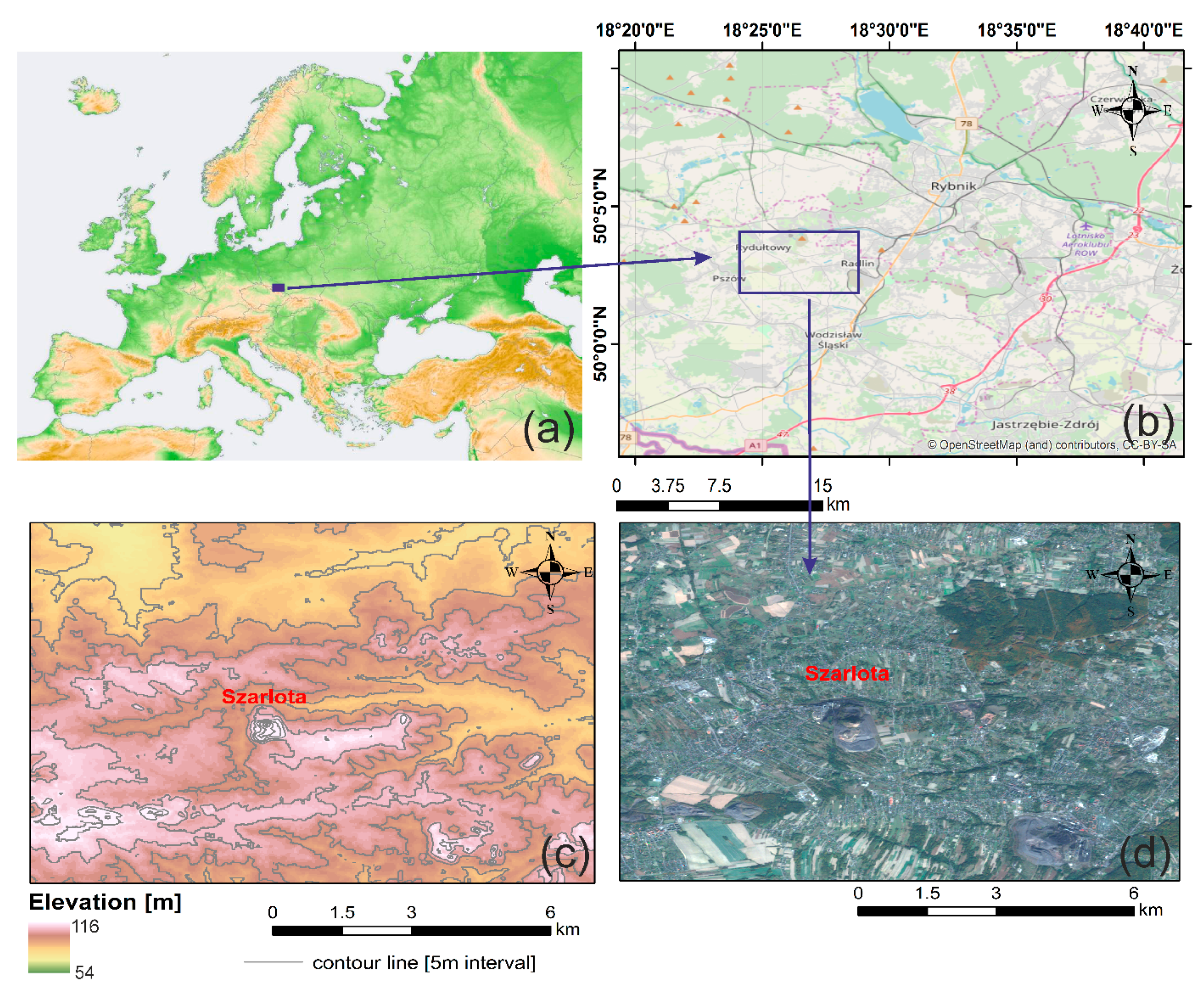
2.1. Study Area

The Rydułtowy mine is located in the southwest part of the Upper Silesian Coal Basin (USCB). The USCB, located in Poland, is one of the largest hard-coal-mining regions in Europe. It covers an area of over 6000 km² in Southern Poland [7,32]. The Rydułtowy mine is the oldest active mining plant in Upper Silesia, with beginnings that date back to 1792. The average daily production of the Rydułtowy mine ranges from 9000 to 9500 t/day, and it is expected to maintain its production capacity at a similar level in the coming years. The location of the study area (32 km²) is presented in Figure 1. The study area is mainly covered by urban and agricultural areas, and a small percentage is covered by wastelands. Coal activity cover an area equal to 75% of the Rydułtowy town. The “Szarlota” slag heap, which is formed by post-mining waste, is 134 m height and the biggest one in Europe [32]. It covers an area of 37 hectares and has a volume of 13.3 million m³. The expected subsidence due to mining activity can exceed a meter per year. Coal exploitation is carried out at depths that range from 800 to 1000 m beneath the ground surface, with depths sometimes reaching 1000–1200 m. The deepest mine workings are located at a depth of 1210 m. Last year, many highly energetic mining tremors were recorded, and many buildings were damaged; however, they are still inhabited [32]. Thus, monitoring deformation in the Rydułtowy region is a crucial issue [32].

2.2. Data Used

In this research, we used 106 ascending and 112 descending Sentinel-1A/B TOPSAR images (C-band) that cover the Rydułtowy mine with a 6-day revisit period. Images cover the period from 4 January 2017 to 8 October 2018 and from 1 January 2017 to 4 November 2018 for the ascending and descending orbit, respectively. This period was selected in order to additionally investigate deformations of the second stage of movements (see introduction) and, in consequence, to build an integrated deformation model by using DInSAR and SBAS results.

Table 1. Metadata about the data used in the presented study.

	Parameters	Description
SAR dataset 1	Product type	Sentinel-1 SLC IW	Sentinel-1 SLC IW
	Track number	175	124
	Mean incidence angle on the study area (degree)	38.11	35.56
	Azimuth angle (degree)	81.77	−77.70
	Orbit mode	Ascending	Descending
	Time span	4 January 2017–8 October 2018	1 January 2017–4 November 2018
SAR dataset 2 (used for evaluation)	Product type	Sentinel-1 SLC IW	Sentinel-1 SLC IW
	Track number	175	124
	Mean incidence angle on the study area (degree)	38.11	35.56
	Azimuth angle (degree)	81.77	−77.70
	Orbit mode	Ascending	Descending
	Time span	April 2015–September 2015	Aprirl 2015–September 2015
Leveling data	Time span	April 2015–October 2015
	Acquired from	The main mining authority
Relative humidity and precipitation data	Time span	1.1.2017–31.12.2018
	Acquired from	https://danepubliczne.imgw.pl/

presents the basic characteristic of the data used. Moreover, we obtained leveling data from the Central Mining Institute for April 2015 and October 2015. However, leveling data have not been acquired since 2015 because of the time and resources needed to perform such measurements. Therefore, for external evaluation, we additionally utilized 14 ascending and 13 descending Sentinel-1A/B TOPS SAR images for the year 2015. The three arc-second (90 m) Shuttle Radar Topography Mission (SRTM) DEM provided by the National Aeronautics and Space Administration (NASA) was utilized to remove the topographic phase component. Precise Orbit Determination (POD) data were provided by the European Space Agency and applied for orbital refinement and phase re-flattening.

3. Methods

We estimated the deformation rate over the Rydułtowy mine by using two SAR techniques, namely (1) classical multi-temporal consecutive DInSAR and (2) the SBAS technique firstly presented by [23]. Figure 2 presents the methodology that we applied in this study. Deformation estimation from two diverse interferometric techniques allowed us to cross-compare the achieved results and mutually strengthen the results of one technique by those of the other technique in a complementary manner. LOS displacements from the SBAS and DInSAR technique were integrated by using the Kriging prediction method. Afterward, we carried out deformation decomposition from both interferometric results. Finally, we evaluated the obtained results internally and externally. Interferometric processing was carried out in SarScape software, while modeling and postprocessing was carried out in Matlab and ArcGIS. A more detailed description of each intermediate step is provided in the following subsections.

3.1. InSAR Processing

3.1.1. Multi-Temporal Consecutive DInSAR Processing

The fundamentals of the classical DInSAR method have been presented in many studies [33,34]. Thus, we do not describe interferometric principles in this work. Many studies have demonstrated the effective application of DInSAR for monitoring fast terrain displacements [4,5,6,7,8]. DInSAR provides reliable results when the displacement rate is much higher than atmospheric artifacts [35]. Despite these atmospheric artifacts, studies have effectively applied conventional DInSAR techniques [4,9,33]. Two methods of DInSAR exist, namely consecutive DInSAR and cumulative DInSAR. The cumulative DInSAR technique is characterized by a fixed master image and the subsequent selection of a slave image (e.g., φ_1-2, φ_1-3, φ_1-4, …, φ_1-n). This approach is very sensitive to temporal decorrelation, which usually increases in the subsequent slave images. In contrast, in the consecutive DInSAR technique, differential interferograms of adjacent SAR acquisitions are calculated and accumulated to provide complete time-series interferometric results (e.g., φ_1-2, φ_2-3, φ_3-4, …, φ_n-1,_n). This technique uses low temporal baselines (6 days by combining Sentinel 1A/B), which minimize temporal decorrelation [36]. However, this strategy also has some limitations. If some errors appear in any of the estimated displacements (residual terrain, atmospheric delay, and other phases error) in the interferograms, then they propagate in the subsequent time-series deformation results in the accumulation process [31]. Nevertheless, many studies have reported the successful application of consecutive DInSAR for subsidence monitoring [4,7,33,36].

After co-registration, 105 and 106 differential interferograms were calculated with a 6-day temporal baseline, and the simulated phase corresponding to the topography was subtracted from the SRTM DEM with 90 m pixel resolution.

Phase unwrapping was performed by using the minimum-cost flow function, and then the unwrapped phase was converted into displacements by means of the following well-known equation:

$$d_{LOS}=\frac{\lambda ·d\varphi }{4\pi }$$

(1)

To minimize atmospheric artifacts, we screened up our differential interferograms, and those ones with clear atmospheric errors were removed from the stack. Auxiliary data about precipitation and humidity from meteorological stations close to the study area were utilized for this purpose. Finally, we removed 33 ascending and 15 descending images from the queue of consecutive DInSAR. The broad overview of methodologies used to reduce atmospheric artifacts can be found in [37]. Based on [38], the investigation of errors related to ionospheric delay has been omitted due to small study area.

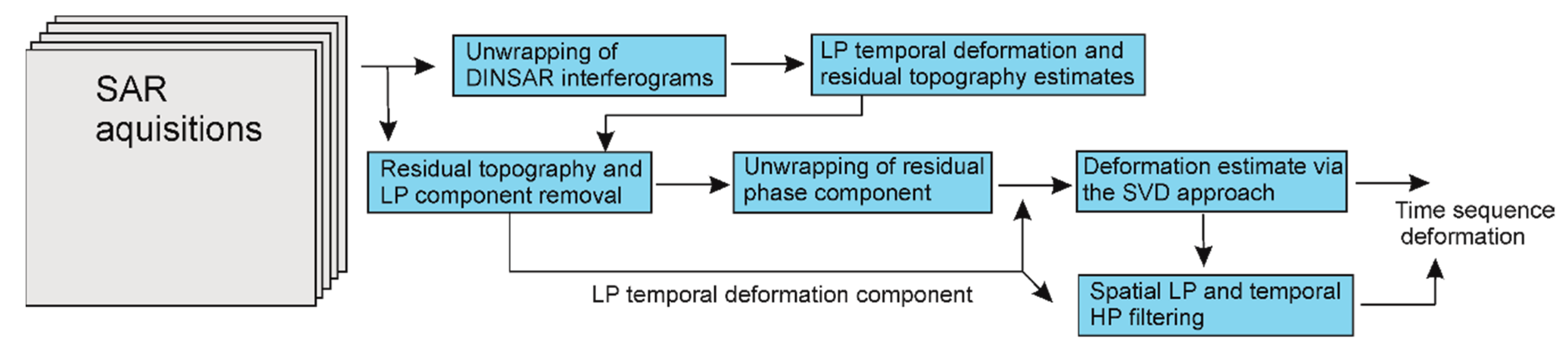
3.1.2. Small BAseline Subset Approach

At the beginning of the XXI century, TS-InSAR techniques were invented to overcome the limitation of conventional DInSAR techniques. The differential phase of two coherent pixels in the range (x) and azimuth coordinates (r) in the interferogram j that is created by two SAR acquisitions at times t_B and t_A is determined as follows:

$$\begin{array}{ll}\delta {\varphi }_j\left(x,r\right)& =\varphi \left(t_B,x,r\right)-\varphi \left(t_A,x,r\right)\\ & \approx \frac{4\pi }{\lambda }\left[d\left(t_B,x,r\right)-d\left(t_A,x,r\right)\right]+\frac{4\pi }{\lambda }\frac{B_{\perp }\Delta z}{Rsin\theta }\\ & +\left[{\varphi }_{atm}d\left(t_B,x,r\right)-{\varphi }_{atm}d\left(t_A,x,r\right)\right]+{\Delta }_{n_j},\hspace{1em}\forall j=1,\dots ,M\end{array}$$

(2)

where λ is a sensor wavelength; $\varphi \left(t_B,x,r\right)$ and $\varphi \left(t_A,x,r\right)$ are the phases that correspond to times $t_A$ and $t_B$; $d\left(t_B,x,r\right)$ and $d\left(t_A,x,r\right)$ are the radar LOS projection of cumulative deformation; $\Delta z$ corresponds to topographic error; ${\varphi }_{atm}d\left(t_B,x,r\right)$ − ${\varphi }_{atm}d\left(t_A,x,r\right)$ is a reference as an atmospheric phase component; $B_{\perp }$ is a perpendicular baseline between two acquisitions; R is the range distance; $\theta$ is the incidence angle; and ${\Delta }_{n_j}$ represents noise and decorrelation effects.

In general, TS-InSAR, by processing multiple acquisitions in time, separates diverse interferometric components that correspond to deformation, topographic error, atmospheric error, and orbital errors [7]. Among the TS-InSAR techniques, the Small BAseline Subset (SBAS) [23] is probably one of the most extensively used techniques [29]. The key advantage of SBAS compared with other TS-InSAR techniques is that SBAS generates interferograms from appropriately selected pairs to minimize the spatial and temporal baseline between two acquisitions orbits. This mitigates the decorrelation problem that occurs with longer baselines [39]. The main steps involved in SBAS processing are presented in Figure 3.

The same datasets were used for both DInSAR and SBAS processing. The overall processing workflow included the following steps: connection graph creation, interferogram generation, Goldstein interferogram filtering, orbital refinement and re-flattening, removal of the atmospheric and topographic error, phase unwrapping, and phase-to-displacement conversion [40]. In the presented study, the normal baseline constraints were used as a percentage of the critical baseline. In light of this, the percentage of the normal baseline was set to 2% of the critical baseline. Additionally, the maximum temporal baseline constraint was set to 30 days for both SBAS processing steps (in ascending and descending orbit). These constraints allowed us to minimize possible geometric (baseline) decorrelation. The system automatically screens the super-master images. Among these, 80 and 88 master images were selected from among 106 and 112 images in ascending and descending orbit, respectively. As a result, five slave images on average were assigned to each master image (this value changes as a result of temporal gaps). Therefore, 80 subsets were created in which, apart from the master image, there were 3–6 slave images. Finally, 442 pairs for ascending orbit and 463 pairs for descending orbit were subjected to further processing. Following co-registration, interferogram generation, and the removal of the flat-Earth phase component due to the Earth’s curvature, Goldstein filtering [41] was applied to remove interferogram noise. We used a predefined cubic displacement model to remove phase residuals from DEM inaccuracies [23], thereby jointly estimating the DEM error and the low-pass (LP) displacement parameters (Figure 3). It is worth highlighting that the SBAS approach removes phase residuals from DEM inaccuracies by estimating the low-pass displacement parameters. Without any a priori knowledge about deformation, a simplified model (which assumes a linear, constant-rate phase variation with time) is typically applied. The linear deformation is adequate for steady-state displacement with respect to image acquisitions. In mining-related subsidence especially, the deformation pattern cannot be described by a linear trend. Rather high nonlinearity has to be expected. Therefore, on the basis of observed DInSAR deformation time series, the cubic model was used for further processing. Depending on the redundancy of the interferogram pairs that met the coherence threshold requirement, minimum-cost flow (MCF) was used to unwrap the phase values. In the SBAS approach, the atmospheric artifacts were modeled by using high-pass and low-pass filtering of the interferograms. This filtering is the so-called atmospheric phase screen (APS). The APS has a stochastic nature, which means that the atmospheric component is highly correlated in space but poorly correlated in time (the weather changes quickly) [23]. We screened the obtained interferograms, and interferometric pairs that had low coherence (<0.3) and/or unwrapping errors were eliminated from further processing. In-depth information on the SBAS algorithm was provided in [23,36].

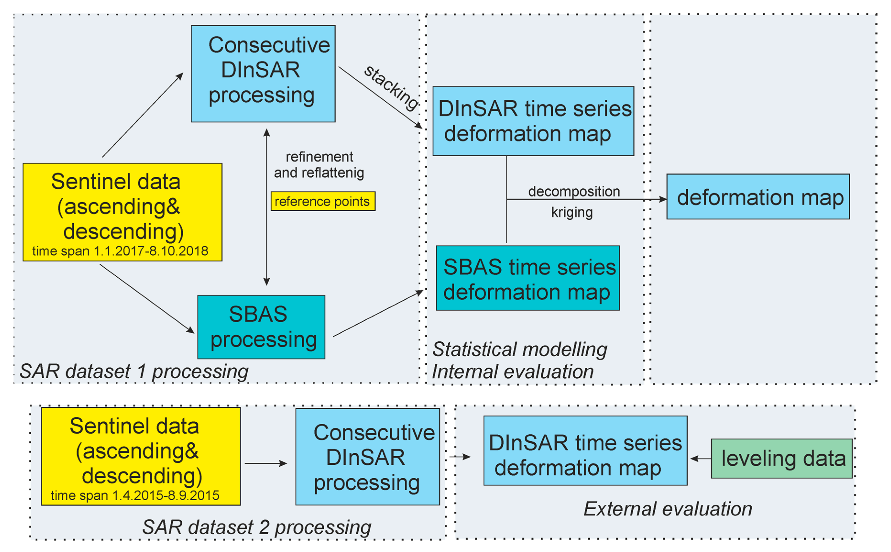
3.2. DInSAR and SBAS Integration

Due to the low coherence, large deformation gradient, and unwrapping problems or not proper deformation model applied in InSAR processing, our DInSAR and SBAS consist of many no-data pixels. In order to generate a continuous deformation map from intermittent SBAS and DInSAR results, we applied the Kriging method. Kriging is a geostatistical prediction method that minimizes the error variance by using a weighted linear combination of the data. The weights are based not only on the distance between the measured points and the prediction location but also on the overall spatial arrangement among the measured points [42]. The spatial autocovariance must be quantified to apply this spatial arrangement in the weights. The special autocovariance in Kriging is described by using an empirical semivariogram [43], which is then approximated by a model using the weighted least-squares fit. In this model, we applied optimization to minimize the mean square error. We converted the raster images generated from the SBAS and DInSAR results into points, which were then used for Kriging interpolation. Each point is located in the centroid of the raster’s pixels. However, since we were aware that the DInSAR results might provide some residual errors, DInSAR points were used only in the areas for which the SBAS results did not provide any information. This integration procedure was independently performed for the ascending and descending orbit obtained from the DInSAR and SBAS results, respectively. For the geostatistical study, we used ArcGIS software. The exponential semivariogram model was applied, and the nugget effect was avoided. To evaluate the predicted maps, we applied the “leave-one-out” technique, which is also known as cross-validation.

3.3. LOS Deformation Decomposition

Radar geometry is only able to measure the path length difference in its Line of Sight (LOS) or slant-range direction. Therefore, DInSAR- derived displacements represent the 1D deformation along the LOS direction. LOS represents the direction/distance between the SAR sensor and the target at hand. This is an essential limitation of SAR systems; thus, several works have been carried out to resolve 2D and 3D displacements from DInSAR measurements [44]. It is possible to retrieve 2D measurements (along-track and in the LOS) [40] by using a multi-aperture InSAR approach or by applying an offset-tracking approach [41]. Diverse methods for 3D decomposition from ascending and descending orbits have been reported in the literature [45,46,47,48,49,50]. A broad overview was presented in [48]. When data from ascending and descending orbit are available, it is possible to retrieve vertical and east-to-west horizontal components. In this work, we applied the equation provided by [51] to calculate the deformation components.

$$d_r=d_u\cos \left({\theta }_{inc}\right)-\sin \left({\theta }_{inc}\right)[d_n\cos \left({\alpha }_h-\frac{3\pi }{2}\right)+d_e\sin \left({\alpha }_h-\frac{3\pi }{2}\right)]$$

(3)

where $d_r$ is the slant-range component in the LOS direction; $d_u$, $d_n$, $\mathrm{and}{d}_e$ are the up, north, and east components of the displacement vector; ${\alpha }_h$ is the heading (azimuth); ${\alpha }_h-\frac{3\pi }{2}$ is the angle to the azimuth look direction; and ${\theta }_{inc}$ is the incidence angle.

Because three unknowns appear in Equation (4), and only two known $d_r$ components are derived from ascending and descending orbit, we were not able to retrieve the full displacement vector ($d_u$, $d_n$, $d_e$). With the Sentinel-1 data over the study area, ${\theta }_{inc}$ ≈ 38°, and ${\alpha }_h$ ≈ 80°, it is easy to observe that Sentinel-1 data are insensitive to north–south displacement detection because of the north orbit direction. Therefore, we assumed that $d_n$ = 0, and this allowed us to find another two components of the deformation vector. This is, of course, a simplification because additional data are lacking; however, as presented in [49], if the investigated deformation has greatly deviated from the N–S direction, which can occur in cases such as subsidence/uplift or a N–W trending fault, it is recommended to neglect the N–S component in the estimation. This is mostly because, in the nonpolar regions, the N–S surface displacements contribute little to the DInSAR-delivered LOS measurements. However, if only some N–S deformations contribute to the estimated LOS measurements and each of the three deformation components is not resolved, then the difference between real and estimated components will be large. This was confirmed in [50], which reported that when a solution with N–S displacements is included in the estimation of the three deformation components, the root-mean-square error (RMSE) between the estimated and real deformation will improve in comparison the RMSE resulting from the use of only two deformation components.

3.4. Validation Methods

After the generation of the final deformation map of the study area, it is desirable to evaluate the InSAR-provided deformation estimates. These estimates cover the period that was chosen to supplement the stage with the most intensive deformations. However, because no other external measurements for the processed period were available, our evaluation was performed differently. Firstly, we performed an internal evaluation and compared the SBAS and DInSAR results. Secondly, we compared the results determined by Kriging with the measured results from SBAS and DInSAR. Besides this, we acquired leveling data for 2015. Since the number of acquisitions was limited, we were able to process them by using only the DInSAR approach. Therefore, an external evaluation was performed only for DInSAR. A more detailed explanation of the validation is presented in Section 5.

4. Results

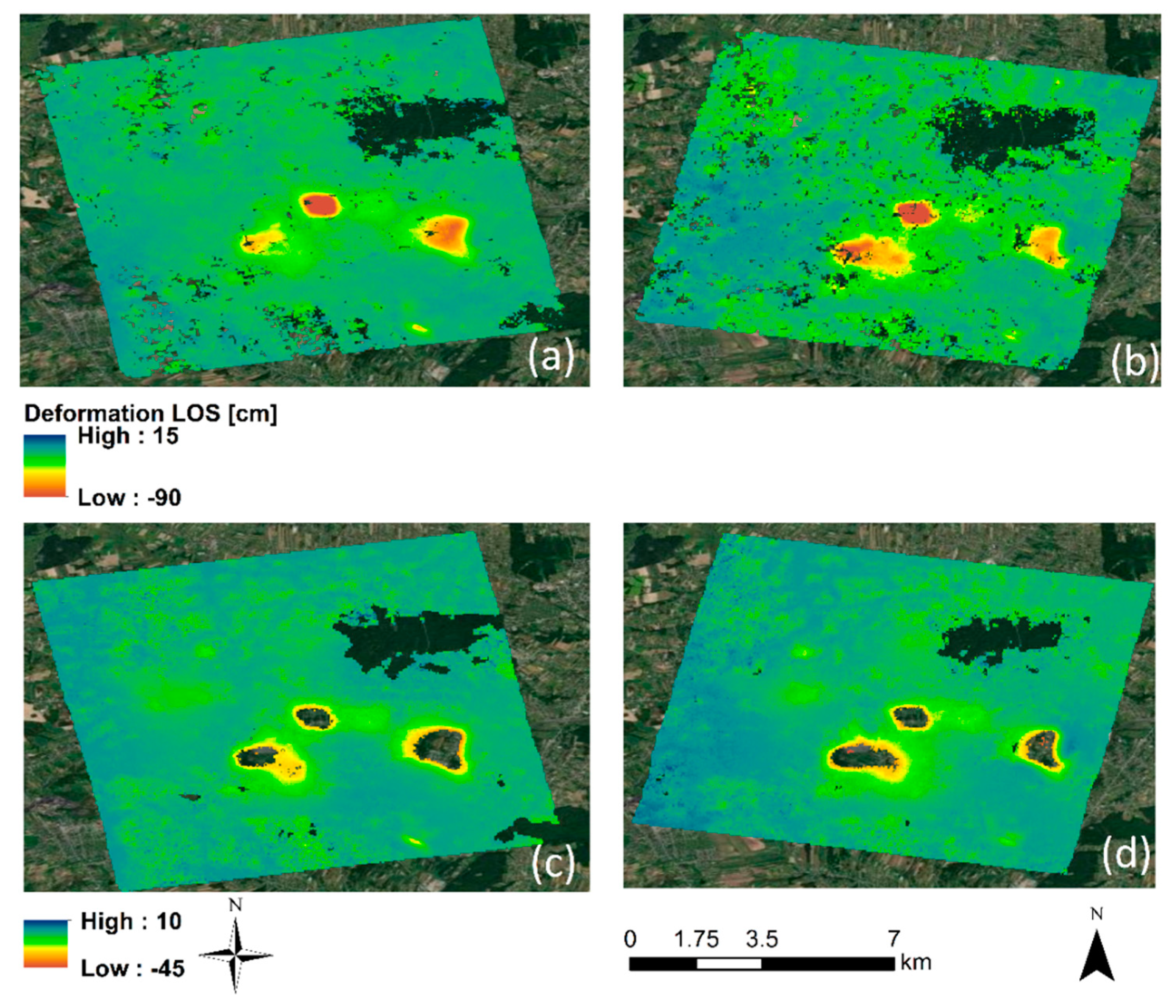
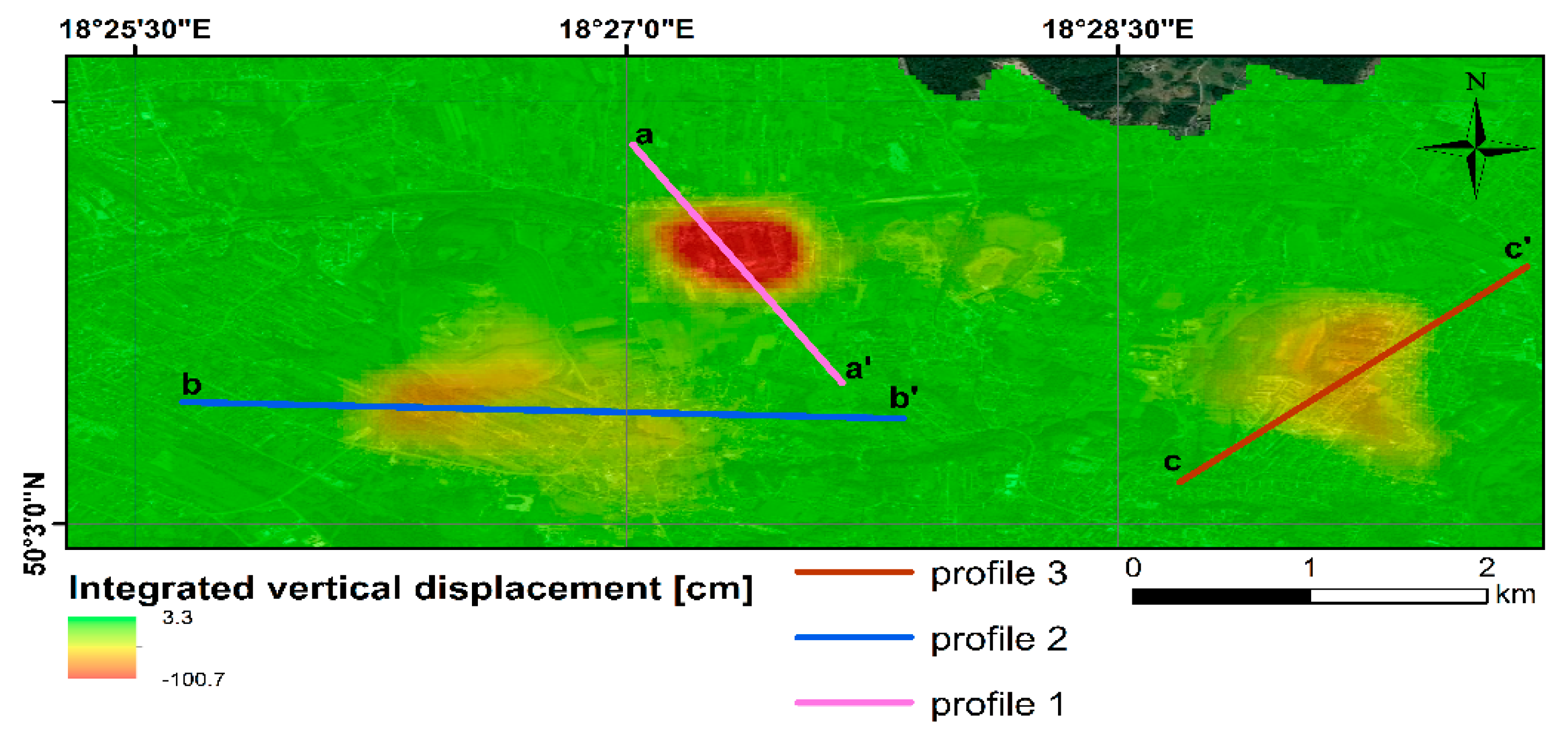
4.1. LOS-Estimated Deformation

Results from DInSAR processing of descending images were refined by trend removal. Since the differences between SBAS and DInSAR are caused by residual errors, for these differences, we fitted polynomial surface. This surface was afterward removed from DInSAR descending results. This approach allowed for the removal of some systematic errors from DInSAR results. Below, in Figure 4, we present the differences between DInSAR and SBAS results for ascending (a) and for descending (b) images. As can be observed, for ascending orbit, the error distribution is symmetric and similar to the normal distribution, while for the descending orbit, the distribution is not symmetric and is affected by some systematic error; in other words, deviations between SBAS and DInSAR contain not only random errors but also systematic components generated by not-handled DInSAR atmospheric errors. After the trend removal from the DInSAR descending results, the mentioned systematic errors are not present, and the distribution is close to normal distribution (Figure 4a). Therefore, for further processing, we have used DInSAR results after the trend removal. Since the trend removal from ascending orbit did not help in error reduction (Figure 4a), for further processing, we used ascending data without the trend removal.

Consecutive DInSAR and SBAS processing resulted in the final displacement maps in the LOS direction for the period between 1 January 2017 and 8 October 2018 for ascending and descending orbit, respectively (Figure 5). Based on Figure 5, a good agreement between the deformation patterns resulting from SBAS and DInSAR is observed. Unfortunately, due to the high deformation gradient or temporal decorrelation, SBAS results provide empty holes in the centers of the subsidence bowls. In contrast, with consecutive DInSAR approach, we were able to detect maximal deformation effectively (especially in the center of the subsidence bowls) in locations that appear as empty holes in the SBAS result.

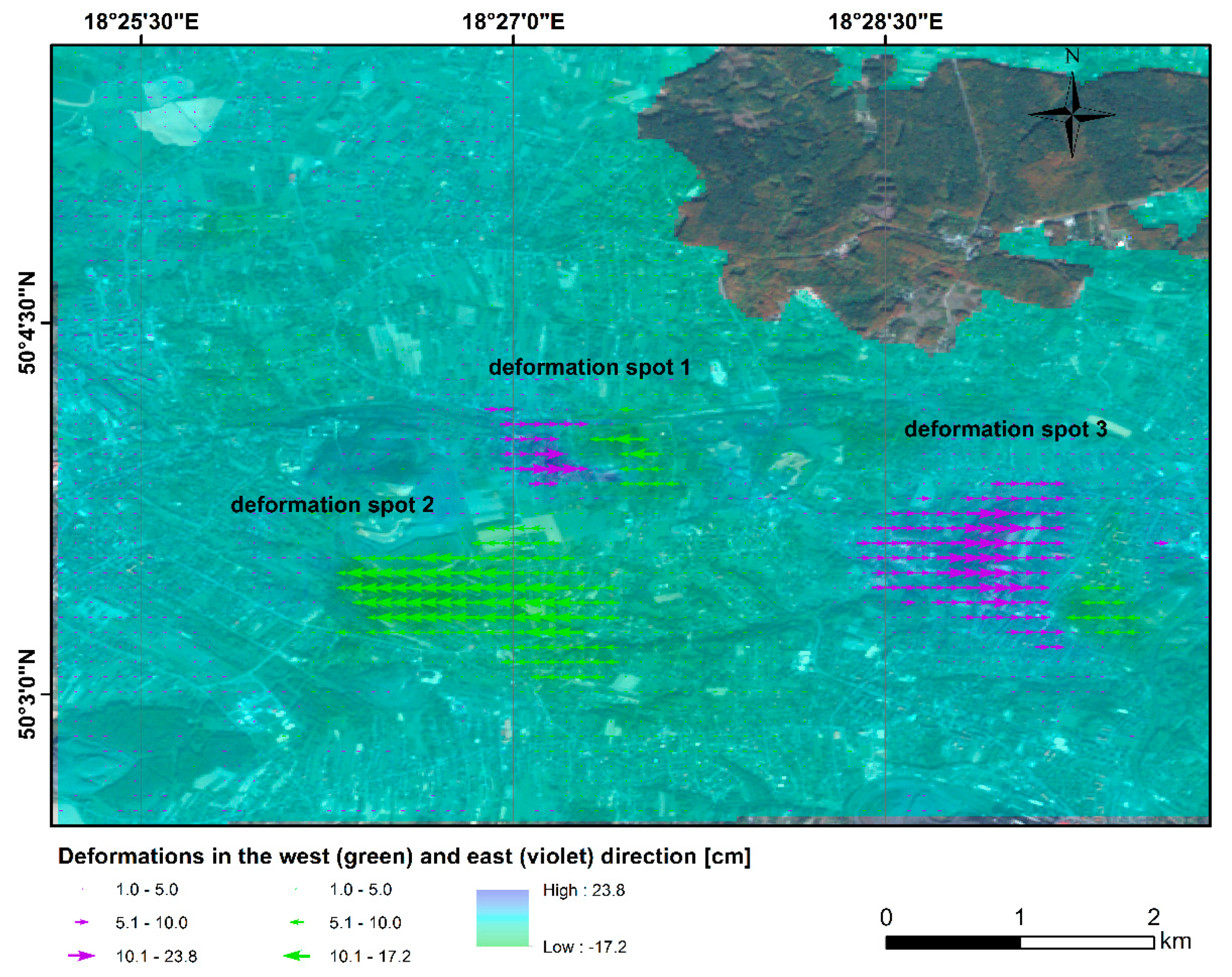
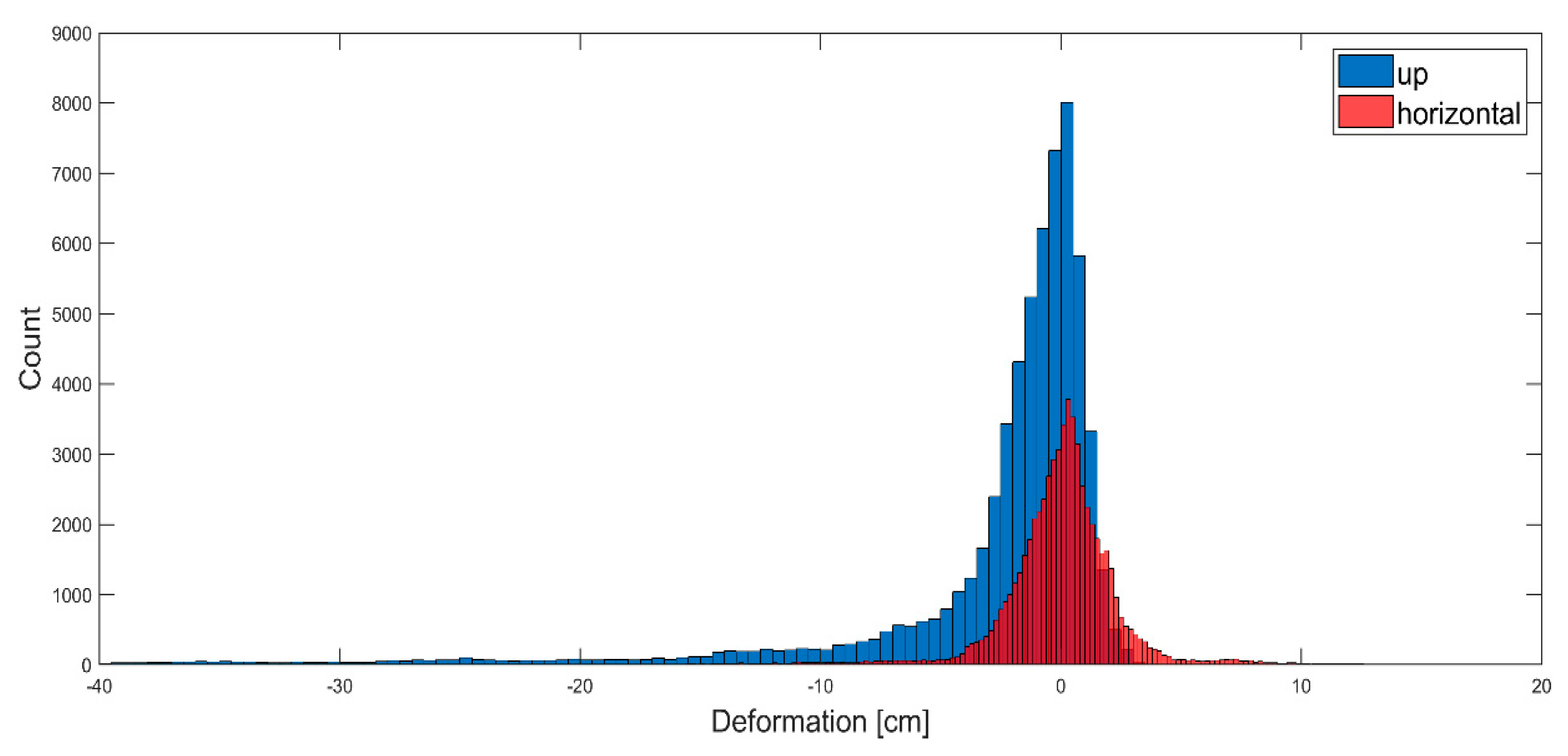
4.2. Estimation of Up–Down and East–West Deformation Components

We used ascending and descending LOS deformation maps to decompose LOS displacements into vertical and horizontal deformation maps, as described in Section 3.3. We performed displacement decomposition for each interferometric pair in the DInSAR and SBAS results. After displacement decomposition, vertical and horizontal maps were added by generating time-series cumulative phase deformation maps. As described in Section 3.4, DInSAR and SBAS vertical and horizontal displacement maps were merged by using the Kriging prediction method. Figure 6 and Figure 7 present the final results of vertical deformation (Figure 6) and horizontal deformation (Figure 7), acquired by integrating SBAS and DInSAR results.

The observation of the difference between ascending and descending orbit clearly indicates existence of horizontal motions (Figure 5). After decomposition (Equation (4)) horizontal displacements are easily observed in the edges of the subsidence bowl. The horizontal deformation component reaches values as high as 24 cm in the east and 17 cm in the west direction. This shows that great care should be taken when interpreting results from only one orbit in mining-related subsidence monitoring. Results for only one geometry could be interpreted as an uplift/subsidence, while this LOS change can correspond to horizontal displacement. This is common in the case of underground mining exploitation, where subsidence edges are slowly moving toward the center of the bowl, while the maximum horizontal deformations are at the edges of the subsidence bowl. The 30 cm values in the east–west direction can be approximated from the relationship between horizontal and vertical components, as presented in [49]. According to this work, the maximum horizontal displacement can be estimated as follows:

$$d_{e_{max}}=b·d_{u_{max}}$$

(4)

The constant $b$ can be estimated by using different parameters, such as the incidence angle, azimuth angle, major influence angle, or mining depth. According to [49], b ranges between 0.3 and 0.4. Given $d_{u_{max}}=1.0$, we can roughly estimate $d_{e_{max}}$, which can range from 0.3 to 0.4 m. These values are confirmed by our results. However, this value is, of course, theoretical, and real horizontal movements strictly depend on the geological and mining conditions. The ideal symmetric location of the east and west component (the same west and east component rate) can rarely be obtained. Different geological units vary in their deformation susceptibility. However, the observed subsequent interferograms indicate that the asymmetric east and west components are due to the existing mine workings. In deformation spot no. 1, these values are quite symmetric, which is not the case for spot no. 2. Comparing the horizontal component with the vertical component, we can observe that asymmetric behavior occurs when vertical deformation does not create a perfectly round subsidence trough. When the subsidence trough is not circle- or ellipse-shaped and has outliers at the edges, then the new coal wall is probably exploited in the area of these outliers. Therefore, the area in which horizontal deformation previously existed is now deforming in a completely different direction, and the perfect symmetric model of the subsidence bowl is no longer preserved. In summary, an asymmetrical shape of the subsidence implies an asymmetrical horizontal deformation component. At this point, it is worth underlining that a mixture of deformation exists in such areas: (1) fast deformation caused by active mining exploitation (outliers from the circle- or ellipse-shaped subsidence trough) and (2) slow deformation due to post-mining exploitation.

In Figure 8, the integrated results from the Kriging-based approach show the distribution of the deformation in both deformation components (up, east–west). East–west deformations almost perfectly fit a symmetric distribution that is close to a normal distribution, while the up components have, as expected, a left-skewed distribution. Most of the values in the integrated results are concentrated around zero, and the dispersion corresponds to the standard deviation estimated in Section 5.1. These values represent stable areas. Thus, the results are appropriately estimated and integrated, and they are free from bias. On the left of the histogram, there is a small interval of approximately equal values (deformations of around −0.1 m). These values and additional values on the left represent deformation within and in the vicinity of the deformation spots.

4.3. Time Series of the Deformation Detected in Three Main Spots

Time-series cumulative deformations estimated using the InSAR integrated approach were extracted for five selected points in the three main deformation spots (see Figure 6). For each selected point, we generated time-series (Figure 9). In spot no. 1 (Figure 9a), subsidence started in September 2017. Between September 2017 and June 2018, total subsidence of 90 cm can be observed, while, for another time range, it does not exceed 10 cm. In spot no. 2 (Figure 9b), subsidence occurred throughout the whole analyzed period at varying velocities over time. A similar situation is evident in spot no. 3 (Figure 9c), but the velocity was more variable in this case. Figure 9 (especially (a) and (c)) support the justification for the selection of the period of interest, as described in Section 2.2.

5. Interferometry Reliability Assessment

Because of the lack of field data for the investigated period, we performed a three-level reliability assessment of the obtained results. RMSE for each evaluation level was calculated. First evaluation level involves RMSE₁ calculation between the SBAS and the DInSAR results. We selected three profiles across the subsidence basins, and we compared the results obtained by SBAS and DInSAR in the LOS direction for both ascending and descending orbit. Second evaluation level involves RMSE₂ calculation between predated deformation, using Kriging and measured deformation from SBAS and DInSAR. Finally, the third evaluation level compared the detected mining-induced deformation with seismic events. All of these evaluations can be regarded as an internal accuracy assessment. For the external evaluation, we used leveling data. However, leveling data were only available for the period from April to October 2015. Therefore, only this time span was evaluated, and only decomposed vertical consecutive DInSAR could be compared with leveling data. A detailed description of each reliability assessment is provided in the following subsections.

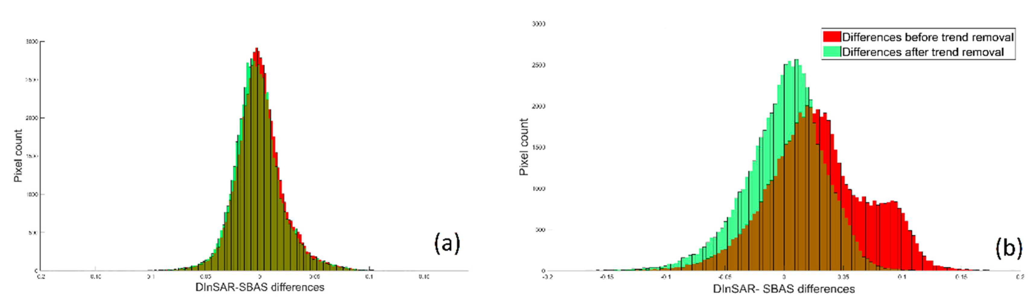
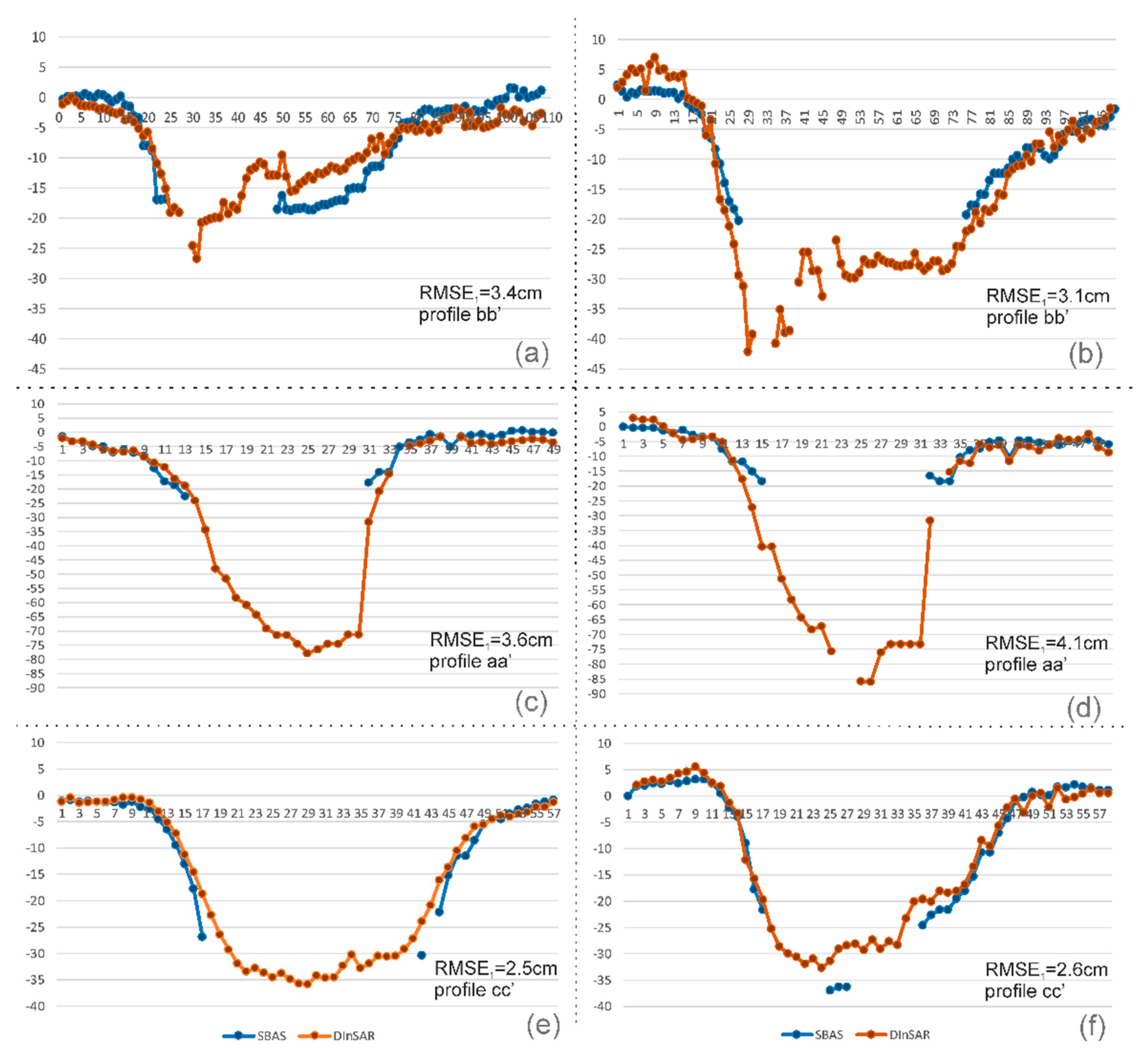
5.1. Cross-Comparison of DInSAR and SBAS Results

With cumulative deformation maps for DInSAR and SBAS, differential map Δd = (d_SBAS − d_DInSAR) for both the ascending and descending geometry in the LOS can be created. The differences in pixels were determined for locations in which both techniques provided deformation values. Otherwise, nonvalues were set for the respective pixel. Of course, in the ideal error-free situation, the differential models for both the ascending and descending cases would output values equal to zero for each pixel. In a real-world scenario, Δd represents residual deformations that are due to all non-compensated and random errors, and we can suppose that the predominant component of Δd is generated by DInSAR. We analyzed these values in terms of the normal distribution. A quantile-to-quantile (q–q) plot was used for this purpose.

A q–q plot is a graphic method that allows us to assess whether sample data belong to the normal distribution. For this reason, quantiles of the sample data are plotted versus quantiles of the theoretical normal distribution. The first step in q–q plot construction is ordering the sample data from the smallest (k = 1) to the largest (k = n), where n is the number of samples, and then plotting these values against expected values of the normal distribution at each quantile in the sample data. The ordered value of k estimates the (k − 1/2)/n quantile of the sample data. The points of q–q plot follow the straight line if the distribution of the sample data is close to the normal distribution.

Q–q plots for both orbit geometries are presented in Figure 10, in which the distributions of residual deformations are clearly symmetric in both cases. Moreover, the residual deformations for the descending orbit (Δd_d) follow an almost-perfect normal distribution in the middle. However, the tails, especially that on the left side, reveal significant deviations from the reference model distribution. We observed that this is the result of gross residual deformations (Δd_d) that appear at the borders of large subsidence bowls. The residual deformations for the ascending orbit (Δd_a) also follow a normal distribution in the middle, but the range of the normal distribution is smaller than in the descending case (Figure 10, right). In both cases, the distribution of residual deformations is tailored; we can consider it as heavy tailored in the case of ascending orbit. The presence of residual deformation values bigger than theoretical values resulting from the normal distribution indicate the appearance of blunders in the deformation determination rather in DInSAR data. Furthermore, we observed that the mentioned blunders appear as pixel groups in the area of infinitesimal deformation (an almost-stable area). With the omission of this area, other locations for the descending orbit, and the whole ascending scene, the residual deformations can be considered randomly distributed.

The mean values of these distributions are close to zero (−0.2 and 0.0 for ascending/descending orbit respectively), wherein, in the case of descending data, it is obvious due to previous trend removal (compare Figure 4). The standard deviations are equal to 2.3 and 3.4 cm for the ascending and descending orbit, respectively

Consequently, we can suppose that cumulative DInSAR results in areas of significant deformation bowls are contaminated mainly by random errors, even if they are caused by the atmospheric artifacts. Thus, our approach, which relies on using only the DInSAR results for the deformation bowls and using the SBAS results for the remaining areas to produce the complete deformation map, seems to be justified at the current research stage. The issue of removing systematic effects and blunders from the DInSAR results will be the subject of future investigations.

Because we used Kriging as a tool to combine DInSAR and SBAS results to produce the final deformation map, it is useful to know the stochastic properties of the scalar field to be modeled. For this reason, the empirical autocovariance function for the differential model Δd of the ascending satellite geometry was calculated. It is clear from Figure 11 that the empirical autocovariance function can be approximated very well with an exponential model. Thus, the use of the exponential covariance model for Kriging is justified.

Furthermore, a more detailed analysis was performed for the area of subsidence basins. The same profile lines in the three subsidence basins (Figure 12) were used to extract the subsidence values in the LOS direction from the DInSAR and SBAS results (Figure 13).

As observed in Figure 13, the results of SBAS- and DInSAR-based measurements coincide with each other fairly well. The same deformation trend is readily apparent. RMSE₁ was calculated for the results of these two interferometric techniques, according to the following equation:

$$RMS{E}_1=\sqrt{\frac{1}{P}{\displaystyle \sum }_{p=1}^p{\left(d_{SBAS}-d_{DInSAR}\right)}^2}$$

(5)

where P is the total number of validated points, d_DInSAR is the deformation extracted from DInSAR analysis, and d_SBAS is the deformation extracted from the SBAS technique. RMSE₁ values are presented in Figure 13. This error is likely caused by the residual atmospheric errors in the DInSAR results, and/or other errors are the results of SBAS’s inability to detect “fast” deformation. Therefore, if deformation falls outside the range of −π to π, then the deformation will be underestimated in the SBAS results. From the extracted profiles, it is evident that the greater difference exists for the second subsidence basin, in which vertical deformations reach around −1.0 m.

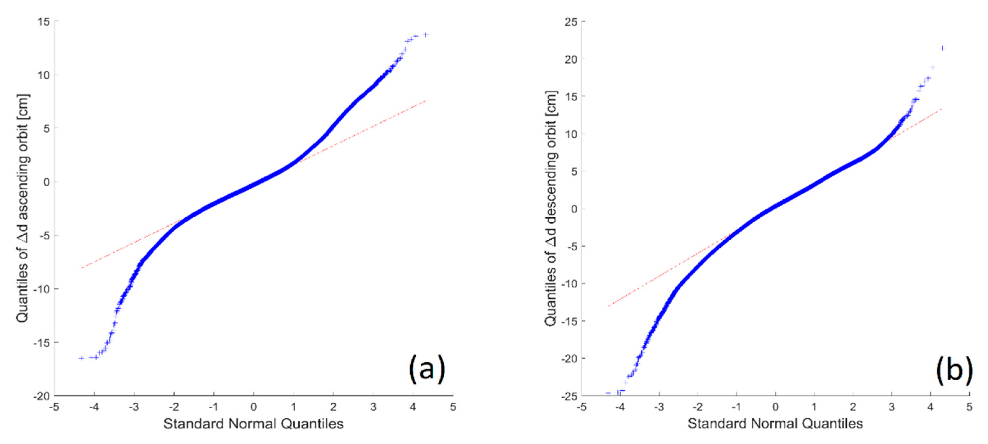
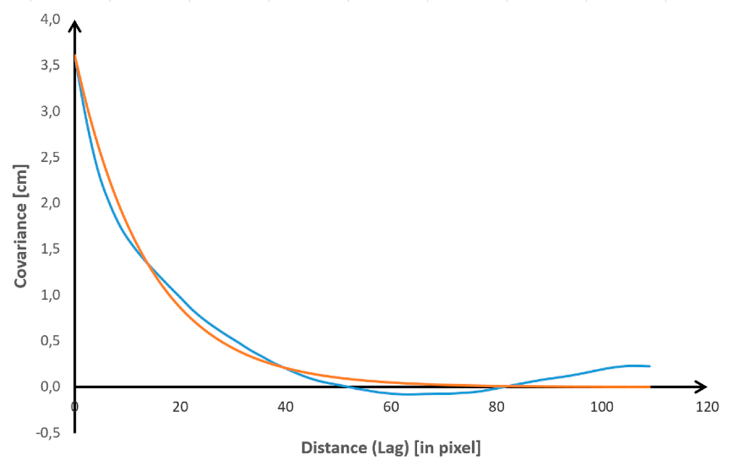
5.2. Internal Evaluation of Kriging-Based Models

As described in Section 3.2, the Kriging geostatistical method was applied for the integration of the SBAS and DInSAR results. For model evaluation, we used a cross-validation procedure to assess the prediction performance of the model. In the cross-validation process, data are predicted by removing one point at a time and predicting the connected data with known values. The predicted point ($\widehat{z}$) and real (z) values at the location of the eliminated point are then compared. Since we want our predictions to be as close to the measured values as possible, RMSE prediction errors are computed as follows:

$$RMS{E}_2=\sqrt{\frac{1}{P}{\displaystyle \sum }_{p=1}^p{\left(\widehat{z}-z\right)}^2}$$

(6)

where P is the total number of validated points, $\widehat{z}$ is the deformation according to the Kriging prediction model, and z is the deformation extracted from InSAR. The values of vertical and horizontal displacements were 11 and 13 mm, respectively. Therefore, the RMSE₂ values resulting from cross-validation indicate that our data-processing scheme is effective.

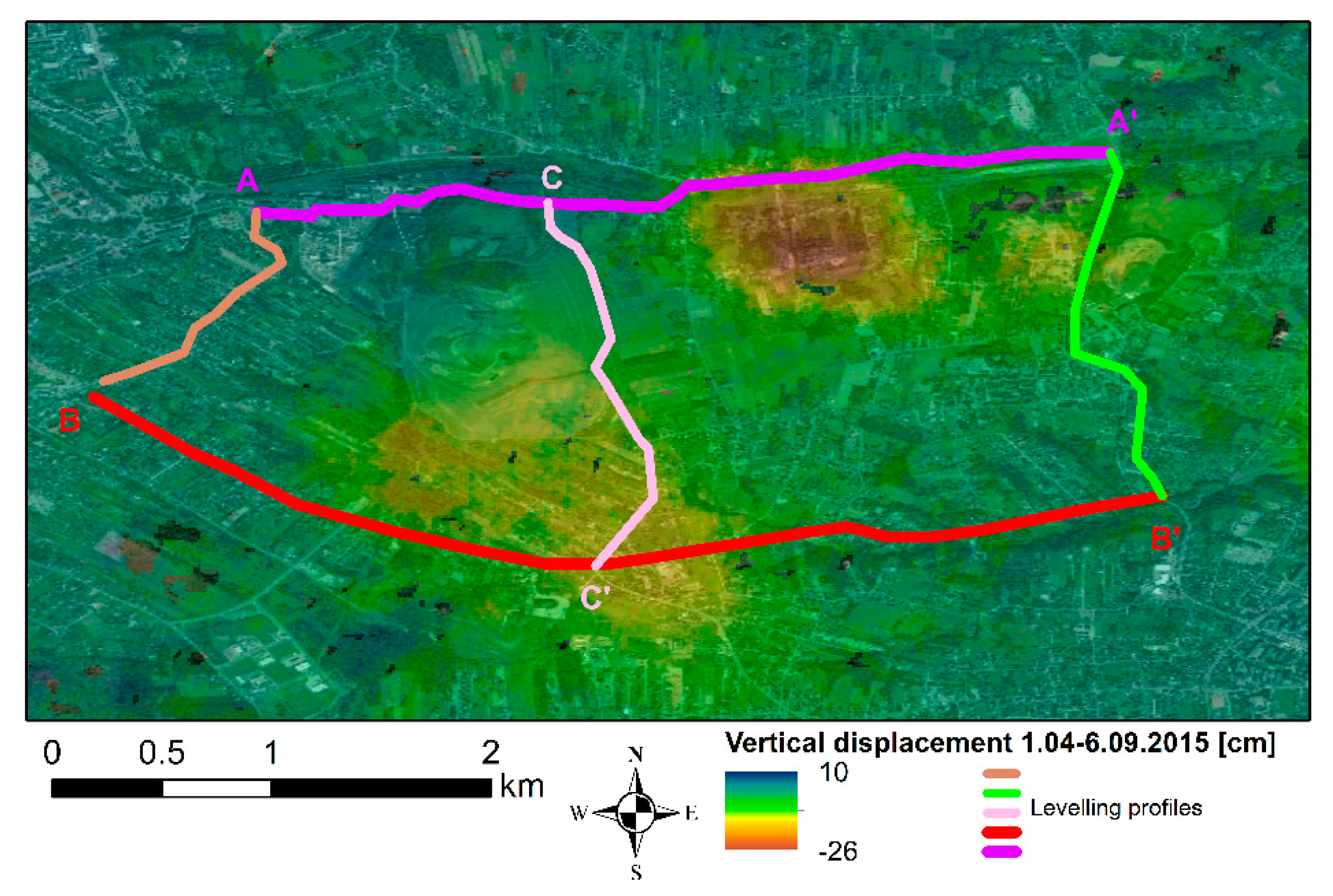
5.3. External Validation

Because the mining authority has not conducted field measurements since 2015, we could not perform an external reliability assessment for displacement monitoring for the timeframe between 1 January 2017 and 8 October 2018. The last leveling measurements were taken in April and October 2015. Unfortunately, during this time, only the Sentinel-1A satellite was operating and had a longer revisit time (12 days), so many temporal gaps exist within the time series. Therefore, because the number of SAR images is limited, the temporal baseline is long, and the temporal data have gaps, SBAS processing could not be performed. Therefore, only the decomposed vertical consecutive DInSAR result was compared with ground survey data. In Figure 14, the leveling lines, together with deformation data extracted from DInSAR, are illustrated. Displacements in 2015 and leveling line measurements performed in April and November 2015.

From the leveling lines, four profiles were selected for the subsidence basins (Figure 15). After decomposition, the vertical displacements extracted from DInSAR processing were compared with the leveling data. In Figure 15, the results of DInSAR-based vertical displacement coincide with leveling data quite well. However, profile 1 shows some discrepancies, especially in the subsidence epicenter.

MSE₃ was calculated for all profiles in order to assess how well the DInSAR results coincide with the leveling data. In this case, RMSE₃ was calculated as follows:

$$RMS{E}_3=\sqrt{\frac{1}{P}{\displaystyle \sum }_{p=1}^p{\left(d_{SAR}-d_{lev}\right)}^2}$$

(7)

where P is the total number of validated points, d_SAR is the deformation extracted from DInSAR analysis, and d_lev is the deformation measured by leveling. RMSE₃ was found to be 3.2, 0.9, 1.0, and 1.7 cm for the first, second, third, and fourth profile, respectively. This corresponds to 18%, 11%, 8%, and 13% of the maximum displacement rate measured by geodetic benchmarks. This agrees well for around a six-month period. However, it has to be highlighted that we calculated the DInSAR-based displacement for the time span between 1 April and 8 September 2015. Unfortunately, there is a temporal gap within the data in October, and subsequent acquisition is from the middle of November. Therefore, the error here can also be attributed to the different lengths of the time spans of these two measurements. This suggests that the agreement between the DInSAR and ground survey results is even better than the calculations indicate.

6. Discussion

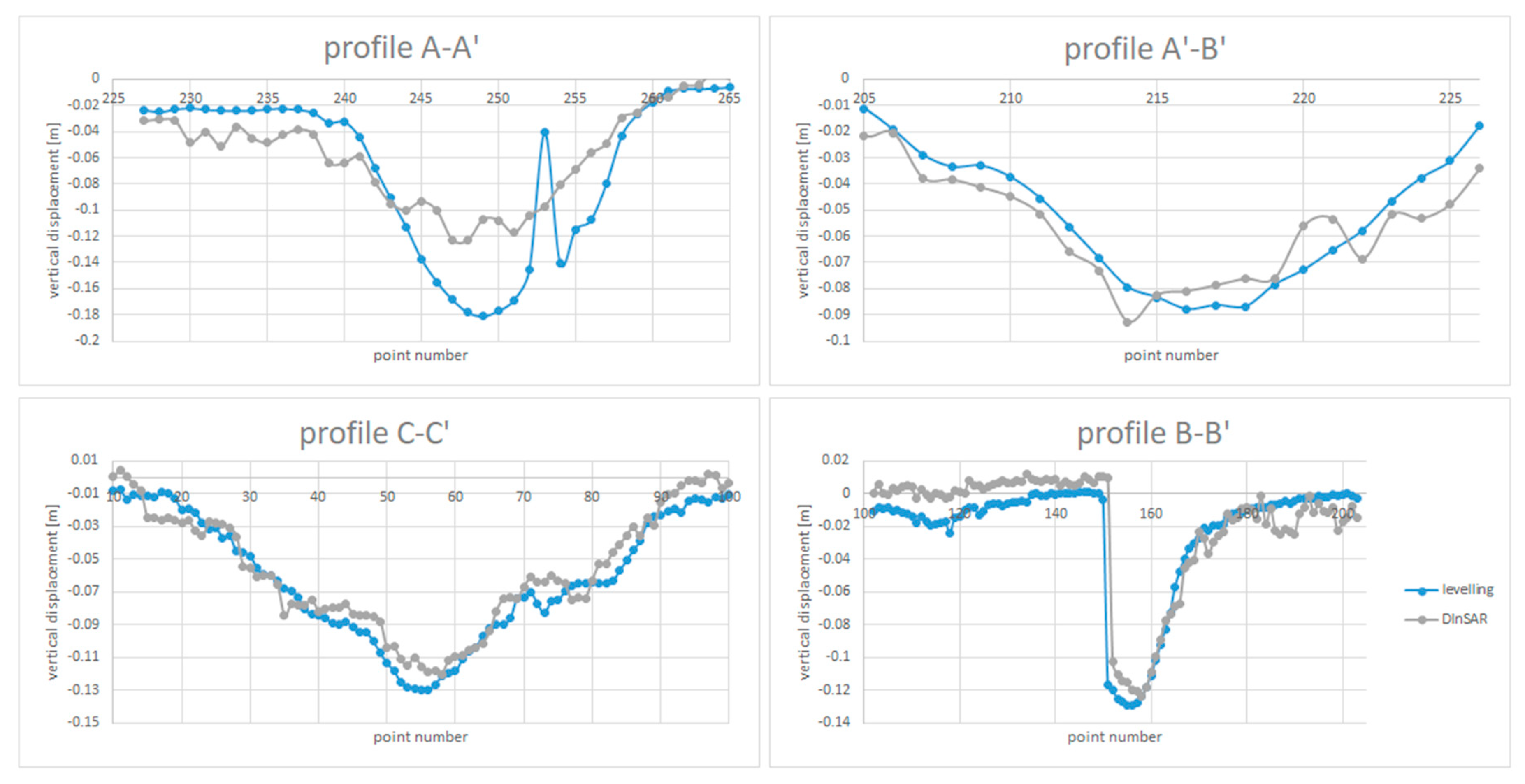
6.1. Comparison between SBAS and DInSAR Deformation Estimation and Comparison with Leveling

The analyses of both the SBAS and DInSAR results identified three main subsidence bowls in the Rydułtowy mine. However, each method has some advantages and disadvantages. The SBAS results failed to estimate displacement in areas with strong displacement located in the central part of a subsidence bowl. As presented in Figure 5, the SBAS technique failed in displacement estimation in the central part of subsidence, where the maximum deformation rate is preserved. This is because of the strong phase discontinuities induced by the large deformation gradient and/or substantial residuals between used deformation model and real deformation pattern. Additionally, the underestimation of displacements occurred in the subsidence bowl, and the reason for that can be the ambiguous nature of the phase [29]. In contrast, consecutive DInSAR was able to capture fast deformation that reached −1.0 m in the vertical direction. Similar results were obtained in [4,7], in which the convergence of DInSAR results and mining modeling for USCB mines was studied. The deformation time series generated for selected points in large deformation spots demonstrate a reasonable agreement with the Knothe mining deformation model (e.g., see [4]) for spots (a) and (c) (Figure 9). This agreement is not evident for spot (b). This is likely because we observed only a small section of the whole deformation process in this spot during the period of investigation. However, the main limitation of DInSAR is the presence of the atmospheric artifacts that directly appear as deformations and are easily observed in stable areas. Therefore, the SBAS technique can be effectively applied in areas of moderate subsidence, such as residual subsidence, which surrounds the subsidence trough. In contrast, the DInSAR approach can be effectively applied to detect fast deformation rates.

As previously stated, each method has some benefits and weaknesses. Cross-comparison of the DInSAR and SBAS approaches (using RMSE₁) was calculated and indicates a good agreement between the DInSAR and SBAS results. The RMSE₁ values correspond to two errors types: (1) the residual atmospheric artifacts that were not removed by elimination of bad images or trend removal and thus preserved in DInSAR displacements; and (2) the inability of SBAS to detect fast displacement and its underestimation of the real magnitude of the displacement. Therefore, after integration by using the Kriging geostatistical interpolation method, RMSE₂ values (13 and 11 mm for vertical and horizontal displacements) indicate that the proposed approach is an excellent solution for monitoring mining-related deformation if the deformation rate is fast, and the temporal decorrelation increases because of intensive mining.

Apart from profiles 1 and 4, DInSAR and the leveling data correspond quite well. An explanation of the differences in the deformation estimation in profiles 1 and 4 could be that we do not know the specific dates of leveling measurements, and some SAR acquisition in October were missing due to a temporal gap in the Sentinel-1 data for October 2015. The difference between these dates and those of the satellite image acquisitions likely inflated RMSE₃.

6.2. Vertical and Horizontal Deformation Components

The explanation for the different values of RMSE₃ could be the location of the profile lines. The second and third profiles are located longitudinally, while the first and fourth are located latitudinally, and their orientation affects the radar sensor’s sensitivity to deformation. Additionally, the first and fourth leveling profiles are located at the edges of the subsidence bowls, which is where the largest horizontal movements occur. With an estimated vertical component of −1.0 m, the horizontal displacement can reach as high as 0.4 m in the east–west and north–south directions. Since we assume the north–south displacement component to be zero during the decomposition step, RMSE₃ is directly affected. This issue was also confirmed by [48]. The main reason for this is that, according to [49], vertical displacement is associated with the sum of the two LOS deformation measurements (ascending and descending), while differences between the two deformation LOS measurements are related to horizontal movements. When we assume that the north–south component is zero when estimating the east–west component (higher sensitivity of the satellite to measure these components), but in reality, some fraction of the north–south component was captured by the satellite, and then the RMSE will be affected. Therefore, although there is a recommendation to neglect the north–south component when it significantly deviates from the north–south direction, having observed the magnitude of the horizontal deformation, we can conclude that the mining-related deformation needs to be modeled in all three deformation components ($d_u$, $d_n$, $d_e$). If the deformation is radially symmetric, the magnitude of N–S displacement would be equal to that for E–W deformation, but at 90 degrees to the E–W deformation. Unfortunately, it is impossible to do so by using only one SAR sensor, and additional SAR data with different imaging geometry (e.g., TerraSAR-X, PALSAR) are needed for this purpose. Alternatively, a method based on a model of mining deformations (e.g., [48,49]) could be considered.

7. Conclusions

In the presented study, the DInSAR and SBAS techniques were integrated to measure mining-related deformation over the Rydułtowy mine in Poland. A total of 106 ascending and 107 descending Sentinel-1 SAR images were processed separately by means of the SBAS and DInSAR approach. The geostatistical Kriging prediction model was applied to integrate the results of these two interferometric techniques. LOS deformations retrieved from ascending and descending geometries were used for 2D displacement decompositions. As a result, three main subsidence basins were detected over the study area, and their vertical and east–west displacements were estimated. The integrated SBAS and DInSAR approach allows for the provision of higher information (spatial) coverage than each technique separately.

The SBAS approach failed to accurately estimate displacement, and this was probably because of temporal decorrelation or the ambiguous nature of the phase. The maximum LOS displacement that was detected using SBAS was −31 cm, −45 cm for ascending and descending orbit, respectively, while the DInSAR technique detected a maximum displacement of −80 cm, −92 cm for ascending and descending orbit. The SBAS technique seems to be reliable for monitoring the residual subsidence that surrounds the subsidence trough, as indicated by the good agreement between the SBAS and DInSAR results in the areas of moderate subsidence. In contrast, the DInSAR approach can detect fast deformation rates.

Because the external data were limited and ground survey results for 2017 were not available, we decided to evaluate the reliability of the DInSAR results for the time span corresponding to leveling data (April 2015 to October 2015). The RMSE₃ values calculated for the four leveling lines (3.2, 0.9, 1.0, and 1.7 cm) and the location of the profiles indicate that the third component of the deformation is not negligible and needs to be modeled for mining-related deformations. However, as a result of the insensitivity of the Sentinel-1 orbit to deformation in the north–south direction, this component has to be modeled by using other modeling techniques or external data (other SAR data).

Finally, having considered RMSE₁, RMSE₂, and RMSE₃, we conclude that the accuracy of the presented approach should not be worse than 4 cm. This indicates that presented approach, as a cost-effective and complementary method to conventional geodetic techniques, can be effectively applied for the monitoring of fast mining subsidence. In the presented study area (Rydułtowy mine), for which leveling measurements are lacking, the presented approach can complement the measurement gaps that exist in leveling survey data and provide regular deformation measurements. Having considered the achieved results and relativity of DInSAR measurements (related to the reference points/ master images, etc.), the DInSAR technique is not an ideal stand-alone technique for deformation monitoring. This method should be compared, calibrated, and supported by another kind of measurements, especially when 3D deformation components need to be acquired (GPS, leveling, LiDAR, etc.)

References

1. Jung, H.C.; Kim, S.W.; Jung, H.S.; Min, K.D.; Won, J.S. Satellite observation of coal mining subsidence by persistent scatterer analysis. Eng. Geol. 2007, 92, 1–13. [Google Scholar] [CrossRef]
2. Borecki, M.; Ochrona, P.P.; Szkodami, G. Surface Protection against Mining Damage; Wydawnictwo Śląsk: Katowice, Poland, 1980; pp. 1–967. [Google Scholar]
3. Perski, Z. ERS InSAR data for Geological Interpretation of Mining Subsidence in Upper Silesian Coal Basin in Poland. In Proceedings of the FRINGE’99 2nd International Workshop on SAR Interferometry, Liege, Belgium, 10–12 November 1999. [Google Scholar]
4. Ilieva, M.; Polanin, P.; Borkowski, A.; Gruchlik, P.; Smolak, K.; Kowalski, A.; Rohm, W. Mining Deformation Life Cycle in the Light of InSAR and Deformation Models. Remote Sens. 2019, 11, 745. [Google Scholar] [CrossRef] [Green Version]
5. Jarosz, A.; Karmis, M.; Sroka, A. Subsidence development with time—Experiences from longwall operations in the Appalachian coalfield. Int. J. Min. Geol. Eng. 1990, 8, 261–273. [Google Scholar] [CrossRef]
6. Ge, L.; Chang, H.C.; Rizos, C. Mine subsidence monitoring using multi-source satellite SAR images. Photogramm. Eng. Remote Sens. 2007, 73, 259–266. [Google Scholar] [CrossRef]
7. Przyłucka, M.; Herrera, G.; Graniczny, M.; Colombo, D.; Béjar-Pizarro, M. Combination of conventional and advanced DInSAR to monitor very fast mining subsidence with TerraSAR-X Data: Bytom City (Poland). Remote Sens. 2015, 7, 5300–5328. [Google Scholar] [CrossRef] [Green Version]
8. Krawczyk, A.; Grzybek, R. An evaluation of processing InSAR Sentinel-1A/B data for correlation of mining subsidence with mining induced tremors in the Upper Silesian Coal Basin Poland. E3S Web Conf. EDP Sci. 2018, 26, 00003. [Google Scholar] [CrossRef] [Green Version]
9. Du, Z.; Ge, L.; Li, X.; Ng, A.H.M. Subsidence monitoring in the Ordos basin using integrated SAR differential and time-series interferometry techniques. Remote Sens. Lett. 2016, 7, 180–189. [Google Scholar] [CrossRef]
10. Gudmundsson, S.; Sigmundsson, F.; Carstensen, J. Three-dimensional surface motion maps estimated from combined interferometric synthetic aperture Radar and GPS data. J. Geophys. Res. 2002, 107, 2250–2264. [Google Scholar] [CrossRef]
11. Massonnet, D.; Feigl, K.L. Radar interferometry and its application to changes in the Earth’s surface. Rev. Geophys. 1998, 36, 441–500. [Google Scholar] [CrossRef] [Green Version]
12. Liu, Z.G.; Bian, Z.F.; Lei, S.G.; Liu, D.L.; Sowter, A. Evaluation of PS-DInSAR technology for subsidence monitoring caused by repeated mining in mountainous area. Trans. Nonferrous Met. Soc. China 2014, 24, 3315. [Google Scholar] [CrossRef]
13. Ng, A.H.-M.; Ge, L.; Du, Z.; Wang, S.; Ma, C. Satellite radar interferometry for monitoring subsidence induced by longwall mining activity using Radarsat-2, Sentinel-1 and ALOS-2 data. Int. J. Appl. Earth Obs. Geoinf. 2017, 61, 92–103. [Google Scholar] [CrossRef]
14. Ciampalini, A.; Solari, L.; Giannecchini, R.; Galanti, Y.; Moretti, S. Evaluation of subsidence induced by long-lasting buildings load using InSAR technique and geotechnical data: The case study of a Freight Terminal (Tuscany, Italy). Int. J. Appl. Earth Obs. Geoinf. 2019, 82, 101925. [Google Scholar] [CrossRef]
15. Farolfi, G.; Del Ventisette, C. Monitoring the Earth’s ground surface movements using satellite observations: Geodynamics of the Italian peninsula determined by using GNSS networks. In Proceedings of the 2016 IEEE Metrology for Aerospace (MetroAeroSpace), Florence, Italy, 22–23 June 2016; pp. 479–483. [Google Scholar]
16. Solari, L.; Del Soldato, M.; Bianchini, S.; Ciampalini, A.; Ezquerro, P.; Montalti, R.; Moretti, S. From ERS 1/2 to Sentinel-1: Subsidence monitoring in Italy in the last two decades. Front. Earth Sci. 2018, 6, 149. [Google Scholar] [CrossRef]
17. Hooper, A.; Bekaert, D.; Spaans, K.; Arıkan, M. Recent advances in SAR interferometry time series analysis for measuring crustal deformation. Tectonophysics 2012, 514, 1–13. [Google Scholar] [CrossRef]
18. Ferretti, A.; Prati, C.; Rocca, F. Nonlinear subsidence rate estimation using permanent scatterers in differential SAR interferometry. IEEE Trans. Geosci. Remote Sens. 2000, 38, 2202–2212. [Google Scholar] [CrossRef] [Green Version]
19. Ferretti, A.; Prati, C.; Rocca, F. Permanent scatterers in SAR interferometry. IEEE Trans. Geosci. Remote Sens. 2001, 39, 8–20. [Google Scholar] [CrossRef]
20. Hooper, A.; Zebker, H.; Segall, P.; Kampes, B. A new method for measuring deformation on volcanoes and other natural terrains using InSAR persistent scatterers. Geoph. Res. Lett. 2004, 31, L23611. [Google Scholar] [CrossRef]
21. Werner, C.; Wegmuller, U.; Strozzi, T.; Wiesmann, A. Interferometric point target analysis for deformation mapping. In Proceedings of the IGARSS 2003 IEEE International Geoscience and Remote Sensing Symposium. Proceedings (IEEE Cat. No. 03CH37477), Toulouse, France, 21–25 July 2003; Volume 7, pp. 4362–4364. [Google Scholar]
22. Kampes, B.; Adam, N. The STUN algorithm for persistent scatterer interferometry. In Proceedings of the FRINGE 2005 Workshop Procs, Frascati, Italy, 28 November–2 December 2005. [Google Scholar]
23. Berardino, P.; Fornaro, G.; Lanari, R.; Sansosti, E. A new algorithm for surface deformation monitoring based on small baseline differential SAR interferograms. IEEE Trans. Geosci. Remote Sens. 2002, 40, 2375–2383. [Google Scholar] [CrossRef] [Green Version]
24. Mora, O.; Mallorquí, J.J.; Broquetas, A. Linear and nonlinear terrain deformation maps from a reduced set of interferometric SAR images. IEEE Trans. Geosci. Remote Sens. 2003, 41, 2243–2253. [Google Scholar] [CrossRef]
25. Crosetto, M.; Crippa, B.; Biescas, E. Early detection and in-depth analysis of deformation phenomena by radar interferometry. Eng. Geol. 2005, 79, 81–91. [Google Scholar] [CrossRef]
26. Fornaro, G.; Pauciullo, A.; Serafino, F. Deformation monitoring over large areas with multipass differential SAR interferometry: A new approach based on the use of spatial differences. Int. J. Remote Sens. 2009, 30, 1455–1478. [Google Scholar] [CrossRef]
27. Rune, T.; Shanker, P.; Zebker, H. A Combined Small Baseline and Persistent Scatterer InSAR Method for Resolving Land Deformation in Natural Terrain; IGC: Oslo, Norway, 2008. [Google Scholar]
28. Ferretti, A.; Fumagalli, A.; Novali, F.; Prati, C.; Rocca, F.; Rucci, A. A new algorithm for processing interferometric data-stacks: SqueeSAR. IEEE Trans. Geosci. Remote Sens. 2011, 49, 3460–3470. [Google Scholar] [CrossRef]
29. Crosetto, M.; Monserrat, O.; Cuevas-González, M.; Devanthéry, N.; Crippa, B. Persistent scatterer interferometry: A review. ISPRS J. Photogramm. Remote Sens. 2016, 115, 78–89. [Google Scholar] [CrossRef] [Green Version]
30. Jia, H.; Liu, L. A technical review on persistent scatterer interferometry. J. Mod. Transp. 2016, 24, 153–158. [Google Scholar] [CrossRef] [Green Version]
31. Yang, Z.; Li, Z.; Zhu, J.; Yi, H.; Hu, J.; Feng, G. Deriving dynamic subsidence of coal mining areas using InSAR and logistic model. Remote Sens. 2017, 9, 125. [Google Scholar] [CrossRef] [Green Version]
32. Pilecka, E.; Szermer-Zaucha, R. Analiza rozkładu szkód górniczych po wysokoenergetycznych wstrząsach z dnia 21 kwietnia 2011 r. i 7 czerwca 2013 r. w kopalni “Rydułtowy-Anna” na tle lokalnej tektoniki. Przegląd Górniczy 2015, T.71 Nr 1, 74–82. [Google Scholar]
33. Perski, Z. Applicability of ERS-1 and ERS-2 InSAR for land subsidence monitoring in the Silesian coal mining region, Poland. Int. Arch. Photogramm. Remote Sens. 1998, 32, 555–558. [Google Scholar]
34. Ng, A.H.-M.; Ge, L.; Yan, Y.; Li, X.; Chang, H.C.; Zhang, K. Rigos Mapping accumulated subsidence using small stack of SAR differential interferograms in the Southern coalfield of New South Wales, Australia. Eng. Geol. 2010, 115, 1–15. [Google Scholar] [CrossRef]
35. Mora, O.; Arbiol, R.; Palà, V. ICC’s project for DInSAR terrain subsidence monitoring of the Catalonian territory. In Proceedings of the IEEE International Geoscience and Remote Sensing Symposium, Barcelona, Spain, 23–28 July 2007; pp. 4953–4956. [Google Scholar]
36. Lanari, R.; Casu, F.; Manzo, M.; Zeni, G.; Berardino, P.; Manunta, M.; Pepe, A. An overview of the small baseline subset algorithm: A DInSAR technique for surface deformation analysis. In Deformation and Gravity Change: Indicators of Isostasy, Tectonics, Volcanism, and Climate Change; Birkhäuser: Basel, Switzerland, 2007; pp. 637–661. [Google Scholar] [CrossRef]
37. Ding, X.L.; Li, Z.W.; Zhu, J.J.; Feng, G.C.; Long, J.P. Atmospheric effects on InSAR measurements and their mitigation. Sensors 2008, 8, 5426–5448. [Google Scholar] [CrossRef] [Green Version]
38. Gomba, G.; González, F.R.; De Zan, F. Ionospheric phase screen compensation for the Sentinel-1 TOPS and ALOS-2 ScanSAR modes. IEEE Trans. Geosci. Remote Sens. 2016, 55, 223–235. [Google Scholar] [CrossRef]
39. Du, Z.; Ge, L.; Li, X.; Ng, A.H.M. Subsidence monitoring over the Southern Coalfield, Australia using both L-Band and C-Band SAR time series analysis. Remote Sens. 2016, 8, 543. [Google Scholar] [CrossRef] [Green Version]
40. Casu, F.; Manconi, A.; Pepe, A.; Lanari, R. Deformation time-series generation in areas characterized by large displacement dynamics: The SAR amplitude pixel-offset SBAS technique. IEEE Trans. Geosci. Remote Sens. 2011, 49, 2752–2763. [Google Scholar] [CrossRef]
41. Fialko, Y.; Simons, M.; Agnew, D. The complete (3-D) surface displacement field in the epicentral area of the 1999 Mw7. 1 Hector Mine earthquake, California, from space geodetic observations. Geophys. Res. Lett. 2001, 28, 3063–3066. [Google Scholar] [CrossRef] [Green Version]
42. Béjar-Pizarro, M.; Guardiola-Albert, C.; García-Cárdenas, R.P.; Herrera, G.; Barra, A.; López Molina, A.; García-García, R.P. Interpolation of GPS and geological data using InSAR deformation maps: Method and application to land subsidence in the alto guadalentín aquifer (SE Spain). Remote Sens. 2016, 8, 965. [Google Scholar] [CrossRef] [Green Version]
43. Johnston, K.; Ver Hoef, J.M.; Krivoruchko, K.; Lucas, N. Using ArcGIS Geostatistical Analyst; Esri: Redlands, CA, USA, 2001; Volume 380. [Google Scholar]
44. Cascini, L.; Fornaro, G.; Peduto, D. Advanced low-and full-resolution DInSAR map generation for slow-moving landslide analysis at different scales. Eng. Geol. 2010, 112, 29–42. [Google Scholar] [CrossRef]
45. Bechor, N.B.; Zebker, H.A. Measuring two-dimensional movements using a single InSAR pair. Geophys. Res. Lett. 2006, 33. [Google Scholar] [CrossRef] [Green Version]
46. Tong, X.; Sandwell, D.T.; Smith-Konter, B. High-resolution interseismic velocity data along the San Andreas fault from GPS and InSAR. J. Geophys. Res. Solid Earth 2013, 118, 369–389. [Google Scholar] [CrossRef] [Green Version]
47. Gourmelen, N.; Kim, S.W.; Shepherd, A.; Park, J.W.; Sundal, A.V.; Björnsson, H.; Pálsson, F. Ice velocity determined using conventional and multiple-aperture InSAR. Earth Planet. Sci. Lett. 2011, 307, 156–160. [Google Scholar] [CrossRef] [Green Version]
48. Hu, J.; Li, Z.W.; Ding, X.L.; Zhu, J.J.; Zhang, L.; Sun, Q. Resolving three-dimensional surface displacements from InSAR measurements: A review. Earth-Sci. Rev. 2014, 133, 1–17. [Google Scholar] [CrossRef]
49. Li, Z.W.; Yang, Z.F.; Zhu, J.J.; Hu, J.; Wang, Y.J.; Li, P.X.; Chen, G.L. Retrieving three-dimensional displacement fields of mining areas from a single InSAR pair. J. Geod. 2015, 89, 17–32. [Google Scholar] [CrossRef]
50. Jianjun, W.Y.L.Z.Z.; Jun, H.U. Coseismic Three-dimensional Deformation of L’Aquila Earthquake Derived from Multi-platform DInSAR Data. Geomat. Inf. Sci. Wuhan Univ. 2012, 7, 25. [Google Scholar]
51. Hanssen, R.F. Radar Interferometry: Data Interpretation and Error Analysis; Springer Science Business Media: Berlin/Heidelberg, Germany, 2001; Volume 2. [Google Scholar]
Figure 1. Location of the study area on the Europe map (a) and Open Street map (b). The bottom images represent the shaded DEM (c) and RGB true color composition from Sentinel 2B acquired on 15 October 2018 (d).
Remotesensing 12 00242 g001
Figure 2. The methodology applied in the presented study.
Remotesensing 12 00242 g002
Figure 3. Small BAseline Subset (SBAS) workflow.
Remotesensing 12 00242 g003
Figure 4. Histograms of differences between SBAS and DInSAR results before (red) and after (green) trend removal for ascending (a) and descending (b) orbits.
Remotesensing 12 00242 g004
Figure 5. SBAS and DInSAR deformation results from the DInSAR (a,b) and SBAS (c,d) technique in the LOS direction for ascending (a,c) and descending (b,d) orbit.
Remotesensing 12 00242 g005
Figure 6. The final vertical displacement map over the Rydułtowy mine between 1 January 2017 and 8 October 2018. The stars refer to extracted time-series deformation in particular deformation spots and are presented in Figure 9.
Remotesensing 12 00242 g006
Figure 7. The final horizontal displacement map over the Rydułtowy mine between 1 January 2017 and 8 October 2018.
Remotesensing 12 00242 g007
Figure 8. The histograms present the vertical (blue) and horizontal (red) displacements (in meters) that were retrieved by using the proposed method (Kriging integration). The drawing is cut off on the left to improve the layout. In fact, there are also single deformations that reach about one meter.
Remotesensing 12 00242 g008
Figure 9. Deformation time series for selected points in the deformation spot: no. 1 (a), 2 (b), and 3 (c).
Remotesensing 12 00242 g009
Figure 10. Quantile–quantile plot of Δd residual deformations for ascending orbit (a) and descending orbit (b) compared with the normal distribution.
Remotesensing 12 00242 g010
Figure 11. Empirical autocovariance function for Δd residual deformations (blue) and the corresponding exponential model (red).
Remotesensing 12 00242 g011
Figure 12. Subsidence bowl with three profiles extracted for DInSAR and SBAS comparison.
Remotesensing 12 00242 g012
Figure 13. Displacement mutual authentication of the estimates of LOS displacement for the two different orbit modes (ascending—left; descending—right) and three diverse subsidence basins. The blue line represents the DInSAR results, while the green line represents SBAS results (in cm).
Remotesensing 12 00242 g013
Figure 14. DInSAR-based vertical displacement verification with leveling data.
Remotesensing 12 00242 g014
Figure 15. Deformation profiles for vertical component of DInSAR results (gray) and leveling (blue).
Remotesensing 12 00242 g015