Novel Approach to Automatic Traffic Sign Inventory Based on Mobile Mapping System Data and Deep Learning


1
Applied Geotechnologies Group, Department Natural Resources and Environmental Engineering, School of Mining and Energy Engineering, University of Vigo, Campus Lagoas-Marcosende, 36310 Vigo, Spain
2
Faculty of Architecture and the Built Environment, Delft University of Technology, 2628 BL Delft, The Netherlands
3
School of Industrial Engineering, University of Vigo, Campus Lagoas-Marcosende, 36310 Vigo, Spain
4
Department Innovation, INSITU Engineering, CITEXVI, Street Fonte das Abelleiras, 36310 Vigo, Spain
*
Author to whom correspondence should be addressed.
Remote Sens. 2020, 12(3), 442; https://0-doi-org.brum.beds.ac.uk/10.3390/rs12030442
Submission received: 10 January 2020
/
Revised: 24 January 2020
/
Accepted: 29 January 2020
/
Published: 1 February 2020
(This article belongs to the Special Issue Advances in Mobile Mapping Technologies)
Abstract
:Traffic signs are a key element in driver safety. Governments invest a great amount of resources in maintaining the traffic signs in good condition, for which a correct inventory is necessary. This work presents a novel method for mapping traffic signs based on data acquired with MMS (Mobile Mapping System): images and point clouds. On the one hand, images are faster to process and artificial intelligence techniques, specifically Convolutional Neural Networks, are more optimized than in point clouds. On the other hand, point clouds allow a more exact positioning than the exclusive use of images. The false positive rate per image is only 0.004. First, traffic signs are detected in the images obtained by the 360° camera of the MMS through RetinaNet and they are classified by their corresponding InceptionV3 network. The signs are then positioned in the georeferenced point cloud by means of a projection according to the pinhole model from the images. Finally, duplicate geolocalized signs detected in multiple images are filtered. The method has been tested in two real case studies with 214 images, where 89.7% of the signals have been correctly detected, of which 92.5% have been correctly classified and 97.5% have been located with an error of less than 0.5 m. This sequence, which combines images to detection–classification, and point clouds to geo-referencing, in this order, optimizes processing time and allows this method to be included in a company’s production process. The method is conducted automatically and takes advantage of the strengths of each data type.

1. Introduction
Communication and mobility of people and goods are key elements of modern societies and developing countries. Economic growth has a huge dependence on and a big relationship with transport networks. Infrastructures such as ports (maritime and river), airports, railways, highways, and roads are among the most relevant transport systems to guarantee the quality of life of people. This relevance is well known by the EU. Proof of that are substantial national and EU funds spent on transport infrastructures every year [1]. These policies are developed based on annual budgets dedicated to new project construction and maintenance of existing infrastructures. In recent times, EU infrastructure policies are changing, focusing more on keeping existing infrastructure in good working condition and less on new construction [2]. This goal has been gathered, among other ways, through different national and EU research work programs (e.g., smart, green, and integrated transport in the case of H2020) [3]. This has promoted numerous activities to improve the service given to society in fields such as monitoring, resilience, reduction of fatal accidents, traffic disruption, maintenance costs, and improvement of network capacity.
Highways and roads are the most used infrastructures for mobility in short distances. As a consequence, their conservation and maintenance show high relevance in terms of safety and secure mobility and reducing associated costs [4,5]. New concepts, called digital infrastructure and Intelligent Transport System (ITS), are being developed in parallel with new concepts for mobility: resilient and fully automated infrastructures; electric, connected and autonomous cars [6].
Concepts of digital infrastructure and ITS are connected. Digital road and permanent monitoring are the bases of any ITS applied to highways and roads to ensure safe mobility and good service conditions. There are different techniques and technologies to achieve digital road monitoring. Depending on the effectiveness and applicability, the most used are based on satellite images, aerial images, and Mobile Mapping System (MMS) solutions.
The low resolution of satellite images makes it impossible to extract certain information from linear infrastructures [7]. Roads, highways, or railways are detectable in the satellite images, but it is not feasible to know the state of the pavement, rails, or their signalling. As a consequence, the scale of work is too small to get effective results with the ITS.
Aerial solutions have grown hugely in recent times based on civil drones and remotely piloted civil systems [8]. This is an emerging market of huge interest. However, drones still have many legal limitations related to the safety and protection of people. These drawbacks limit their use in many fields, among them transport infrastructures.
The MMS solutions, based on Light Detection and Ranging (LiDAR) technology, images (video and panoramic), and GNSS (Global Navigation Satellite System) technologies (for data geolocation) [9], are mature solutions that saw limited growth for mainly two reasons: the high price of the technology and high cost of processing the captured data (in terms of labour cost). Notwithstanding, the market is showing novel and very active emerging low-cost and multiplatform solutions for autonomous vehicles. On the other side, big data and artificial intelligence techniques allow efficient data processing [10].
This work is focused on developing a technical solution to generate infrastructure digital models and road infrastructure inventory based on the MMS. This work is applied to a specific component of roads, i.e., traffic signs (TSs), which are very relevant in transport infrastructures for the safety and security of people. The objective is the fast TS detection, recognition, and classification with accurate localization. But the application field of the proposed method is not limited to TSs. The proposed method shows high relevance for autonomous mobility solutions and urban planning. Based on them, the solution provides key information about on existing traffic signs, including accurate geolocation parameters.
This paper is organized as follows: Section 2 collects related work about traffic sign detection, recognition, and mapping in images and point clouds. Section 3 explains the designed method. Section 4 presents and discusses the results obtained from applying the method to case studies, and Section 5 concludes the work.
2. Related Work
The interest in the off-line automation of traffic sign inventory has increased in recent years. Previously, proposed approaches tackled the particular properties of traffic signs (i.e., retro-reflectivity for night-time visibility, colour, shape, size, height, orientation, planarity, and verticality), usually following safety standards. These properties require traffic signs to be treated as different objects from traffic lights [11,12,13], poles [14], lanes [15,16,17], trees [18], and other objects present in roads. A review of approaches depending on the object can be found in [19].
Traffic sign (TS) current technology provides mainly two sources of data: 3-D georeferenced point clouds acquired through Mobile Laser Scanning (MLS) techniques; and digital images from a still camera or as a frame extracted from a video. 3-D point-cloud data contains precise information related to 3-D location and geometrical properties of the TS, as well as intensity. However, resolution of most MMS techniques under normal use is not accurate enough to recognise all TS classes. Images are used to overcome that weakness as they contain visual properties, despite the lack of spatial information. Since the objective in automated traffic sign inventory is to accurately determine placement in global coordinates and the specific type of each traffic sign on the road, point cloud and image become complementary [20,21,22].
For TS inventory to be automated it is required to follow four main steps: traffic sign detection (TSD), segmentation (TSS), recognition or classification (TSR), and TS 3-D location. TSD aims to identify regions of interest (ROI) and boundaries of traffics signs. In TSS, a segment corresponding to the object is separated from the set of input data. TSR consists of determining the meaning of the traffic sign. Meanwhile, TS 3-D location deals with estimating 3-D position and orientation, or pose, of the TS. A variety of approaches for these steps have been proposed in literature directly or indirectly related to TS inventory.
One group of these approaches defines techniques focused on detecting and segmenting the set of points with spatial information of the TS from 3-D laser scanner point clouds. These techniques are based on the a priori knowledge of 3-D location, geometrical and/or retro-reflective properties. All approaches are conditioned by the huge amount of information contained in point clouds (see, for instance, [23,24,25,26,27,28,29,30]). With the aim of accurate TSR, aforementioned approaches combine point clouds with images to extract features. As a previous step to TSR, segmented points can be projected onto the corresponding 2-D image in the traffic-sign-mapping (TSM) step. A review of methods for TSR in point-cloud and image approaches can be found in [31].
These types of techniques based on TSD in 3-D point cloud and TSR in image are accurate and reliable for TS inventory. However, they entail high time and computational costs, mainly for the TSD and TSS steps. As an alternative, images can be used not only for TSR but also for TSD without making use of the 3-D point cloud. Some authors have used TSD in image for coarse segmentation of the 3-D point cloud [32,33].
TSD, TSS, and TSR in image, which become TSDR, have been extensively studied for TS inventory as well as for other applications such as advanced driver assistance systems (ADAS). The vast variety of techniques proposed by the computer–vision community have been reviewed and compared, detailing advantages and drawbacks, in [34,35,36,37,38]. Recently, Wali et al. [39] provided a comprehensive survey on vision-based TSDR systems.
According to them, in TSDR image-based techniques detection consists in finding the TS bounding box, while recognition involves classification by giving an image a label. Common TSD methods are: colour-based, on different colour spaces, i.e., RGB, CIELab, and HIS [40]; shape-based, such as Hough Transform (HT) and Distance Transform (DT); texture-based, such as Local Binary Patterns (LBP) [41]; and hybrid. By these methods a feature vector is extracted from image with lower computational cost than from 3-D point cloud. Then, the class label of the feature vector is obtained using a classifier such as Support Vector Machine (SVM) or with Deep Learning-based (DL) methods [42,43,44]. Among the latter, Convolutional Neural Networks (CNN) have been widely adopted, given their high performance in both TSD and TSR in images [45,46,47,48] and in point clouds [49].
Regarding TS inventory, TSDR in image requires the TS 3-D location to be completed. TS 3-D location, after TSDR, has been considered by several authors in image-based 3-D reconstruction approaches without making use of a 3-D point cloud. These techniques require prior accurate camera calibration and removement perspective distortion. In [50], 3-D localization is based on epipolar geometry of multiple images, while Hazelhoff et al. [51] calculated the position of the object from panoramic images referenced to northern direction and horizon. Balali et al. [52] built a point cloud by photogrammetry techniques using a three parameter pinhole model. Wang et al. [53] used stereo vision and triangulation techniques. In [54], 3-D reconstruction is conducted by geometric epipolar, taking into account geometric shape of TS.
While TSDR in image is proved as high-performance, reconstruction models for TS 3-D location from image are overcome in precision by 3-D point-cloud-based location. However, little research has paid attention to techniques for TS inventory that jointly takes advantage of TSDR in image and TS 3-D location from the 3-D MLS point cloud. In [32], a method to combine DL with retro-reflective properties is developed for TS extraction and location from a point cloud. In [55], TS candidates are detected on images based on colour and shape features and filtered with point-cloud information. Most authors use point clouds for TSD and images only for TSR [23,24,25,26,28,29].
In contrast to other approaches, in this work a data flow is implemented to minimize processing times by taking advantage of each type of data. First, images are used for TSD and TSR. Image processing is faster than point-cloud processing and allows the application of DL techniques, which right now are state of the art. In addition, the design of a modular workflow allows each network to be replaced in the future as its success rates increase. To maximize a correct TS identification, different networks for TSD and TSR are used, unlike other works that use the same network to detect and classify, see also [44,48]. After image processing, point clouds are used to filter out multiple TS detections and false positives. Point clouds allow more precise geolocation than the use of epipolar geometry of multiple images. Point clouds are not used for detection and classification since:
- DL point-cloud processing techniques are computationally more expensive than their equivalent in image processing.
- The addition of point-cloud data to images increases processing times.
- The low point density does not provide useful information for TSR.
3. Method
The method consists of four main processes. First, TSs are detected in images. Second, detected TSs are recognized. Third, TSs are 3-D geolocated by the projection of detected signs to the point cloud. Fourth, multiple TS detections of the same sign in different images are filtered. The input data of the method are MMS data: images from a 360° camera, point clouds, GPS-IMU positioning data, and camera calibration data. Figure 1 shows the workflow of the method.
3.1. Traffic Sign Detection
TSD is based on object detection in images. No point-cloud data are used at this stage to speed up the detection process. The input images are acquired with a 360° RGB camera mounted on the MMS during acquisition. The panoramic image is converted and rectified into six images oriented according to cube sides. Images in trajectory direction IT provide TS information in front of the MMS. Images in the opposite direction ITo provide TS information in back of the MMS, either in the same lane or in different lanes. Lateral images are perpendicular to trajectory direction I⊥T and provide information about signs located on MMS sides. Lateral images I⊥T are particularly relevant for detecting no-parking signs or no-entry signs. The images forming the top and bottom of the cube are not relevant for TSD. Bottom images are occupied by the camera support. TSs that could be detected on top images are already detected by front images IT.
The object detector implemented in this method is RetinaNet [57]. This detector has been chosen because it is state of the art in standard accuracy metrics, memory consumption, and running times. RetinaNet is a one-stage detector that has good behaviour with unbalanced classes and in images with a high density of objects at several scales, key factors for traffic sign detection. RetinaNet uses ResNet [58] as a basic feature extractor, and in this work is used the ResNet 50.
The RetinaNet detector is applied to each cube-side image I of the set acquired with the MMS during the acquisition. As a result, an array is obtained for each TS detected S(l,Ix,Iy,w,h) where l indicates the label, Ix and Iy indicate top left corner position of the bounding box, w indicates TS width and h indicates TS height. In order to obtain maximum classification accuracy, the number of classes has been reduced to coincide with shapes of traffic sings. The classes for detection with RetinaNet are five: yield, stop, triangular, circular, and square (Figure 1). In the recognition phase (Section 3.2) these classes will be classified.
3.2. Traffic Sign Recognition
In this phase, TSs previously detected by their shape are classified with their final label. In some TSs, their shape coincides with their final class, as in the case of stop signs (octagonal) and yield sign (inverted triangle). TSs of obligation (circular), recommendation–information (square), and danger (triangular) encompass multiple classes that must be classified for a correct inventory. For each of these three sign shapes, an InceptionV3 network [59] has been trained and implemented. The InceptionV3 network needs input samples of fixed size 299 * 299 * 3 pixels, the bounding boxes images of detected signs S are resized to adapt them to the network input.
3.3. Traffic Sign 3-D Location
The projection of TSs detected in images onto the georeferenced point cloud is done using the pinhole model [60]. While in other works the four vertices of the detection polygon have been projected, in this work, only the central TS point is projected Sc. This saves processing time and minimizes calibration error. Another alternative would be detecting the pole directly or after TS detection. Pole detection would mean more precise positioning, but it has the following limitations: (1) poles may not have enough points to be easily detected, (2) some TSs share a pole, and (3) some TSs are located on traffic lights, light posts, or buildings, so specific detection methods are needed for each case. In view of the above, the authors have chosen to consider the error of positioning the TS to the pole as negligible, and obtain a simpler and faster method based on TS location and positioning. The TS location in point cloud PS is done by projecting a line defined by the camera focal point C and the central sign-point Sc (pinhole model in Equation (1)).
where is the scalability factor; is the centre of traffic signal S detected in an image I, with and ; K is the intrinsic camera parameters matrix provided by the manufacturer; is the extrinsic camera parameters matrix; is the centre of the point-cloud traffic signal .
The rotation and translation matrix positions the camera in the same coordinate system as the point cloud Ps, which is already georeferenced. is formed by two rotation–translation matrices relates the positioning of the pixels with the image by calibration prior to implementation of the method. Once the matrix for one image is obtained, it is valid for all images acquired with the same equipment. The calibration is done by manually selecting the four pairs of pixels in images and points in the point cloud per image. positions the camera in the optical centre C of each image I.
The TS points in the point cloud Ps form a plane . The TS is located in the intersection between the projection of the line following the pinhole model and plane (Figure 2), .
In order to reduce processing time, a region of interest (ROI) is delimited in the point cloud to calculate possible planes (Figure 3). First, points located at a distance more than d from the MMS location at the time of taking the image are discarded. Distant TSs from the MMS are considered to have very low point density for correct location. Distant TSs also are detected in successive images captured near the MMS. Second, points located at a larger distance than r from line are discarded. Third, points not located in the image orientation are discarded. TSs detected in images cannot be in a point cloud in a different orientation. For remaining points, planes are detected in order to discard point not in planes. Since TSs are planar elements, planar estimation avoids false locations due to noise points crossing the projection line .
3.4. Redundant Traffic Sign Filtering
Since the same TS can be detected in multiple images, multiple detections of the same TS must be simplified. The filtering is done with information of the classified TS, because one post can contain TSs of different classes. TSs of the same class grouped in a smaller radius than f are eliminated, leaving only the first detected (Figure 4).
4. Experiments
4.1. Equipment and Parametes
The MMS equipment used for this work consisted of a Lynx Mobile Mapper, with a Ladybug5 360° camera and a GPS-IMU Applanix POS LV 520. The cube-images had a resolution of 2448 × 2024 pixels and they were captured with a frequency of 5 m in MMS trajectory. The point cloud was a continuous acquisition over time. The values of parameters d and r to delimit the ROI were set at 15 m and 2 m, respectively. The value of parameter f was set to 1 m in order to simplify duplicate signals.
For the RetinaNet training, 9500 images were used with 12,036 TSs, obtained by the 360° camera and labelled. The training of the InceptionV3 networks was carried out with data sets of Belgium [50], Germany [61], and images of Spanish traffic signs. The whole process (training and testing in real case studies) was executed on a CPU computer Intel i7 6700, 32 GB RAM, GPU Nvidia 1080ti. The code was combined TensorFlow–Python for TSD and TSR and C++ for 3-D location and filtering.
The RetinaNet training consumed 70 h with hyper-parameter optimization method adam, learning rate 1e-5, L2 Regularization 0.001, Max Epochs 50 and Batch Size 1. The hyper-parameters for the three Inceptionv3 training were optimization method sgdm, learning rate 1e-4, Momentum 0.9, Max Epochs 126 and Batch Size 64. The training of the triangular signs required 50 min, 12,995 samples for training and 407 for validation. The training of the circular signs required 80 min, 25,000 samples for training and 743 for validation. The training of the squared signs required 7 min, 1094 samples for training and 243 for validation. The training process in terms of loss per epoch is shown in Figure 5.
4.2. Case Studies
The methodology was tested in two real case studies: two secondary roads located in Galicia (Spain) denominated EP9701 and EP9703. Road EP9701 case study was 9.2 km long, the point cloud contained 350 million points and was acquired with 7392 images. Road EP9703 case study was 5.5 km long, the point cloud contained 180 million points and was acquired with 4520 images. Both roads were located in rural areas where houses, fields, and wooded areas were interspersed. The roads had frequent crossings and curves. The sign-posting of both roads was abundant and in good condition, with few samples that were damaged or partially occluded. The case studies were processed in 30 and 20 min, respectively.
The acquisition was performed at the central hours of the day (to minimize shadows) and on a sunny day without fog, so as not to affect visibility. The MLS maintained a constant driving speed of approximately 50 km/h, although this speed was reduced by following rules at intersections or traffic lights. Point density increased as the driving speed decreased. It was estimated that the points in acquisition direction were 1 cm closer for every 10 km/h that the speed was reduced.
4.3. Results
TS accounting was done manually by reviewing acquired images, detected signals, classified signs and their locations in the point cloud. Table 1 shows the image count for each case study.
TSs were correctly detected at 89.7%, while 10.3 % were not detected. The use of the 360° camera and the cube-images made it possible to locate TSs in the opposite and lateral directions to the MMS movement. Some of the undetected TSs were partially occluded or were eliminated in the redundant TS filtering process (Section 3.4), since they were traffic signs of the same class separated within a distance f. Figure 6 shows examples of detected TSs.
A high percentage of false detections was counted (19.6%). Of these, traffic mirrors represented 81.8% and 37% of false detections in case studies 1 and 2 respectively. Mirrors have a circular shape surrounded by a red ring, so they were detected as false circular signals. Although the use of the point cloud has been considered to eliminate these false positives, since mirrors should not have points due to their high reflectivity, in the case studies the mirrors contained points due to their dirt or deterioration. Nor have any characteristics been found that differentiate mirror points from TS points. The remaining false detections corresponded to different objects on roadsides. Figure 7 shows some examples of false detections.
Duplicate TSs were not filtered due to incorrect positioning by the TS 3-D location process (Section 3.3). In the input cube-side images, 382 TSs were detected in case study 1 and 441 signs in case study 2. After the 3-D localization and redundant filtering processes, the set of detections was reduced to 113 and 137 TSs, respectively. Duplicated TSs were 4.2% of the total.
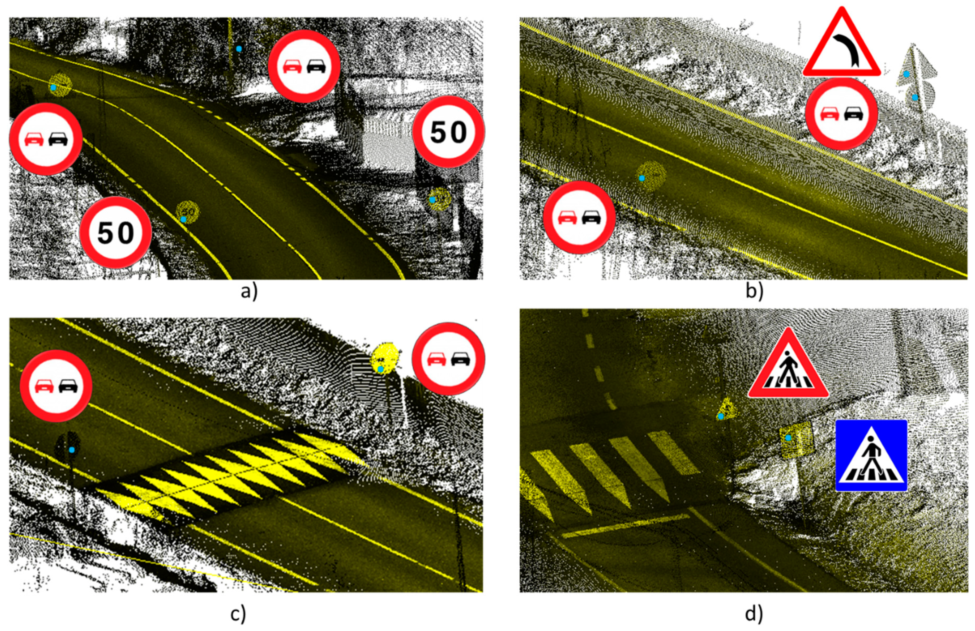
The positioning of a TS was based on the georeferenced point cloud, where the authors assumed that the location of the point cloud corresponded precisely to reality, as in [23]. Authors also considered that the TSs positioned in the correct TS point cloud were correctly located (0 m error). A total 97.5% of the detected TSs corresponded to points belonging to TSs (Figure 8). Only five TSs were positioned with an error of between 0.5 m and 8 m to the real location of the sign. These TSs not correctly positioned in the corresponding TS point clouds were manually measured from their incorrect detected location to the real TS location in the point cloud.
With regard to signal recognition, 92.5% of the detected TSs were correctly classified, both in good condition and partially erased. Since the methodology was tested in real case studies, it was not possible to test all the existing classes of training data. The main classes in the case studies were TSs of dangerous curves, speed bumps, no overtaking, and speed limits. To a lesser extent, there were also traffic signs of yield, stop, roundabouts, no entry, roadworks, and pedestrian crossings. No significant confusion was detected among classes. Errors in confusion were isolated and were corresponded to the results of training.
4.4. Discussion
In general, most TSs were detected and positioned correctly, although the algorithm showed a tendency to over-detection. This behaviour was chosen to facilitate monitoring by a human operator. In a correction process, it was considered easier to eliminate false detections than to check all input data for undetected signals. In terms of false positives per image, the false detection rate was low, 0.004 FP/image, compared to [54], where 0.32 and 0.07 were reached in the cases with images of better resolution. Regarding undetected TSs (false negatives), the neural network did not detect 10.3% of all TSs, which was similar to other artificial intelligence works: 10% in [51] and 11% in [28], but far from the best of the state of the art: 6% in [62], based on laser scanner intensity; 5% in [32], based on combining two neural networks; and 4% in [29], based on bag-of-visual-phrases.
The authors are aware that the detection success rate was not as high as in other applications using RetinaNet [63]. This was due to the relative small size of the data set for TSD and the great variability of elements that existed in the road environment. Generating a data set for detection is a costly work and was not the final objective of this work, which was focused on presenting a methodology composed of a series of processes to inventory signals, and not on optimizing the success rates of Deep Learning networks such as RetinaNet and InceptionV3.
The methodology did not reach detection rates as high as reference works in TSD and TSR, such as [50,52], although it is worth mentioning that the latter classifies TS grouped by type. By contrast, the proposed methodology is adaptable for mapping different objects, as it does not focus on exclusive TS features. Particularly, by not using reflectivity, it was possible to detect TSs whose reflectivity had diminished due to the passage of time and incorrect maintenance. With the use of Deep Learning techniques, although they do not explain exactly why false detections occur, it is possible to intuit the underlying problem. Deep Learning techniques allow continuous improvement and updates to the training database with new samples that, in this case, may be the wrong detections once corrected. In this way, the algorithm will be able to avoid them.
The combination of images to TSD and TSR with a point cloud to TS 3-D locations allowed a precise positioning of 97.5% of detected TSs in points belonging to TS point clouds, which was not reached by other works based exclusively on epipolar geometry of multiple images, such as [50], which only achieved a positioning with 26 cm of average error, [53] with 1-3 m of average error using dual cameras, and [64] with 3.6 m of average error using Google Street View images.
While point clouds provide valuable information for locating objects, they also require much more processing time than images. The methodology designed in [23] for TSD and TSR in point clouds was implemented in the two case studies. Processing times using point clouds has reached 45 and 30 min, respectively. The time increment is 50% more than performing TSD and TSR on images and 3-D location in point clouds, as proposed in this work. No relation was found between inventory quality and driving speed changes during acquisition. The work maintained a driving acquisition speed similar to other point-cloud mapping works.
5. Conclusions
In this work, a methodology for the automatic inventory of road traffic signs was presented. The methodology consists of four main processes: traffic sign detection (TSD), recognition (TSR), 3-D location and filtering. For the TSD and TSR phases, cube-images acquired with a 360° camera were used and processed by Deep Learning techniques. Five shapes of traffic signs were detected in the cube-side images (stop, yield, triangular, circular and square) applying RetinaNet. Since the stop and yield forms each corresponded to only one TS, in order to recognize the other forms in their respective classes, an InceptionV3 network was trained for each classification. For the 3-D location and filtering phases, the georeferenced point cloud of the environment was used. TSs detected in the images were projected onto the cloud using the pinhole model for correct 3-D geolocation. Finally, the duplicate signals detected in different images were filtered based on the coincidence between classes and distance between them. The methodology was tested in two real case studies with a total of 214 TSs, 89.7% of the TSs were correctly detected, of which 92.5% were correctly classified. The false positive rate per image was only 0.004 and main false detections were due to road mirrors. 97.3% of the detected signals were correctly 3-D geolocated with less than 0.5 m of error.
The effectiveness in the combination of data images and point clouds was demonstrated in this work. Images allow the use of artificial intelligence techniques for detection and classification, which improve their success rates day by day with new networks and designs. In addition, image processing is much faster and more efficient than point cloud processing. The use of a 360° camera does not require the passage of the MMS in two road directions. Furthermore, point clouds allow a more precise geolocation of signals than only using images.
The entire process of TS inventorying from processing images (first) and point cloud (continued) ensures speed and effectiveness in processing time, 50% faster than other proposals that first treat point clouds and then images with much higher computational costs which, although they provide satisfactory results in terms of success rates, make their inclusion in production processes unfeasible due to cost of time and computer equipment. Due to these advantages, the presented methodology is suitable to be included in the production process of any company. Also, it is conducted automatically without human intervention.
Future work will focus on extending the methodology to more objects important for road safety and for the inventory of objects, as the methodology does not depend on any exclusive feature of TSs. In addition, it is proposed to feed back the network to improve the success rate of detections with corrected images that present the main types of error. It is also considered to test the methodology in other case studies such as highways and urban roads, to analyse the influence of driving speed during acquisition on 3-D point cloud location.
Author Contributions
Conceptualization, P.A. and D.C.; method and software, D.C.; validation, D.C. and J.B.; investigation, E.G.; resources, P.A.; writing, J.B., E.G. and P.A.; visualization, J.B.; supervision, E.G. and P.A. All authors have read and agreed to the published version of the manuscript.
Funding
This research was funded by Xunta de Galicia given through human resources grant (ED481B-2019-061, ED481D 2019/020) and competitive reference groups (ED431C 2016-038), the Ministerio de Ciencia, Innovación y Universidades -Gobierno de España (RTI2018-095893-B-C21). This project has also received funding from the European Union’s Horizon 2020 research and innovation programme under grant agreement No 769255. This document reflects only the views of the authors. Neither the Innovation and Networks Executive Agency (INEA) or the European Commission is in any way responsible for any use that may be made of the information it contains. The statements made herein are solely the responsibility of the authors.
Acknowledgments
Authors would like to thank to those responsible for financing this research.
Conflicts of Interest
The authors declare no conflict of interest.
References
- European Union EU Funding for TEN-T. Available online: https://ec.europa.eu/transport/themes/infrastructure/ten-t-guidelines/project-funding_en (accessed on 1 June 2019).
- European Commission EC Road and Rail Infrastructures. Available online: https://ec.europa.eu/growth/content/ec-discussion-paper-published-maintenance%5C%5C-road-and-rail-infrastructures_en (accessed on 28 June 2019).
- European Union Horizon 2020 Smart, Green and Integrated Transport. Available online: https://ec.europa.eu/programmes/horizon2020/en/h2020-section/smart-green-and-integrated-transport (accessed on 3 December 2019).
- Balado, J.; Díaz-Vilariño, L.; Arias, P.; Lorenzo, H. Point clouds for direct pedestrian pathfinding in urban environments. ISPRS J. Photogramm. Remote Sens. 2019, 148, 184–196. [Google Scholar] [CrossRef]
- Soilán, M.; Riveiro, B.; Sánchez-Rodríguez, A.; Arias, P. Safety assessment on pedestrian crossing environments using MLS data. Accid. Anal. Prev. 2018, 111, 328–337. [Google Scholar] [CrossRef] [PubMed]
- European Commission Innovating for the Transport of the Tuture. Available online: https://ec.europa.eu/transport/themes/its_pt (accessed on 3 December 2019).
- Quackenbush, L.; Im, I.; Zuo, Y. Road extraction: A review of LiDAR-focused studies. Remote Sens. Nat. Resour. 2013, 9, 155–169. [Google Scholar]
- Leonardi, G.; Barrile, V.; Palamara, R.; Suraci, F.; Candela, G. Road Degradation Survey Through Images by Drone. In International Symposium on New Metropolitan Perspectives; Springer: Cham, Switzerland, 2019; pp. 222–228. ISBN 978-3-319-92101-3. [Google Scholar]
- Soilán, M.; Sánchez-Rodríguez, A.; del Río-Barral, P.; Perez-Collazo, C.; Arias, P.; Riveiro, B. Review of laser scanning technologies and their applications for road and railway infrastructure monitoring. Infrastructures 2019, 4, 58. [Google Scholar] [CrossRef] [Green Version]
- Wirges, S.; Fischer, T.; Stiller, C.; Frias, J.B. Object Detection and Classification in Occupancy Grid Maps Using Deep Convolutional Networks. In Proceedings of the IEEE Conference on Intelligent Transportation Systems, ITSC, Maui, HI, USA, 4–7 November 2018; Volume 2018-Novem. [Google Scholar]
- Fairfield, N.; Urmson, C. Traffic light Mapping and Detection. In Proceedings of the 2011 IEEE International Conference on Robotics and Automation, Shanghai, China, 9–13 May 2011; pp. 5421–5426. [Google Scholar]
- Levinson, J.; Askeland, J.; Dolson, J.; Thrun, S. Traffic Light Mapping, Localization, and State Detection for Autonomous Vehicles. In Proceedings of the 2011 IEEE International Conference on Robotics and Automation, Shanghai, China, 9–13 May 2011; pp. 5784–5791. [Google Scholar]
- Diaz-Cabrera, M.; Cerri, P.; Medici, P. Robust real-time traffic light detection and distance estimation using a single camera. Expert Syst. Appl. 2015, 42, 3911–3923. [Google Scholar] [CrossRef]
- Li, Y.; Wang, W.; Tang, S.; Li, D.; Wang, Y.; Yuan, Z.; Guo, R.; Li, X.; Xiu, W. Localization and Extraction of Road Poles in Urban Areas from Mobile Laser Scanning Data. Remote Sens. 2019, 11, 401. [Google Scholar] [CrossRef] [Green Version]
- Chen, X.; Kohlmeyer, B.; Stroila, M.; Alwar, N.; Wang, R.; Bach, J. Next Generation Map Making: Geo-referenced Ground-level LIDAR Point Clouds for Automatic Retro-reflective Road Feature Extraction. In Proceedings of the GIS, Seattle, WA, USA, 4–6 November 2009; pp. 488–491. [Google Scholar]
- Wan, R.; Huang, Y.; Xie, R.; Ma, P. Combined Lane Mapping Using a Mobile Mapping System. Remote Sens. 2019, 11, 305. [Google Scholar] [CrossRef] [Green Version]
- Gu, X.; Zang, A.; Huang, X.; Tokuta, A.; Chen, X. Fusion of Color Images and LiDAR Data for Lane Classification. In Proceedings of the 23rd SIGSPATIAL International Conference on Advances in Geographic Information Systems, Washington, DC, USA, 3–6 November 2015. [Google Scholar]
- Kang, Z.; Yang, J.; Zhong, R.; Wu, Y.; Shi, Z.; Lindenbergh, R. Voxel-based extraction and classification of 3-D pole-like objects from mobile LiDAR point cloud data. IEEE J. Sel. Top. Appl. Earth Obs. Remote Sens. 2018, 11, 4287–4298. [Google Scholar] [CrossRef]
- Che, E.; Jung, J.; Olsen, M.J. Object recognition, segmentation, and classification of mobile laser scanning point clouds: A state of the art review. Sensors 2019, 19, 810. [Google Scholar] [CrossRef] [Green Version]
- Meierhold, N.; Spehr, M.; Schilling, A.; Gumhold, S.; Maas, H.-G. Automatic feature matching between digital images and 2D representations of a 3D laser scanner point cloud. Int. Arch. Photogramm. Remote Sens. Spat. Inf. Sci. 2010, 38, 446–451. [Google Scholar]
- Gómez, M.J.; García, F.; Martín, D.; de la Escalera, A.; Armingol, J.M. Intelligent surveillance of indoor environments based on computer vision and 3D point cloud fusion. Expert Syst. Appl. 2015, 42, 8156–8171. [Google Scholar] [CrossRef]
- García, F.; García, J.; Ponz, A.; de la Escalera, A.; Armingol, J.M. Context aided pedestrian detection for danger estimation based on laser scanner and computer vision. Expert Syst. Appl. 2014, 41, 6646–6661. [Google Scholar] [CrossRef] [Green Version]
- Soilán, M.; Riveiro, B.; Martínez-Sánchez, J.; Arias, P. Traffic sign detection in MLS acquired point clouds for geometric and image-based semantic inventory. ISPRS J. Photogramm. Remote Sens. 2016, 114, 92–101. [Google Scholar] [CrossRef]
- Arcos-García, Á.; Soilán, M.; Álvarez-García, J.A.; Riveiro, B. Exploiting synergies of mobile mapping sensors and deep learning for traffic sign recognition systems. Expert Syst. Appl. 2017, 89, 286–295. [Google Scholar] [CrossRef]
- Guan, H.; Yan, W.; Yu, Y.; Zhong, L.; Li, D. Robust Traffic-Sign Detection and Classification Using Mobile LiDAR Data With Digital Images. IEEE J. Sel. Top. Appl. Earth Obs. Remote Sens. 2018, 11, 1715–1724. [Google Scholar] [CrossRef]
- Wen, C.; Li, J.; Luo, H.; Yu, Y.; Cai, Z.; Wang, H.; Wang, C. Spatial-related traffic sign inspection for inventory purposes using mobile laser scanning data. IEEE Trans. Intell. Transp. Syst. 2016, 17, 27–37. [Google Scholar] [CrossRef]
- Wu, S.; Wen, C.; Luo, H.; Chen, Y.; Wang, C.; Li, J. Using Mobile LiDAR Point Clouds for Traffic Sign Detection and Sign Visibility Estimation. In Proceedings of the 2015 IEEE International Geoscience and Remote Sensing Symposium (IGARSS), Milan, Italy, 6–31 July 2015; pp. 565–568. [Google Scholar]
- Bruno, D.R.; Sales, D.O.; Amaro, J.; Osório, F.S. Analysis and Fusion of 2D and 3D Images Applied for Detection and Recognition of Traffic Signs Using a New Method of Features Extraction in Conjunction with Deep Learning. In Proceedings of the 2018 International Joint Conference on Neural Networks (IJCNN), Rio de Janeiro, Brazil, 8–13 July 2018; pp. 1–8. [Google Scholar]
- Yu, Y.; Li, J.; Wen, C.; Guan, H.; Luo, H.; Wang, C. Bag-of-visual-phrases and hierarchical deep models for traffic sign detection and recognition in mobile laser scanning data. ISPRS J. Photogramm. Remote Sens. 2016, 113, 106–123. [Google Scholar] [CrossRef]
- Balado, J.; Sousa, R.; Díaz-Vilariño, L.; Arias, P. Transfer Learning in urban object classification: Online images to recognize point clouds. Autom. Constr. 2020, 111, 103058. [Google Scholar] [CrossRef]
- Ma, L.; Li, Y.; Li, J.; Wang, C.; Wang, R.; Chapman, A.M. Mobile laser scanned point-clouds for road object detection and extraction: A review. Remote Sens. 2018, 10, 1531. [Google Scholar] [CrossRef] [Green Version]
- You, C.; Wen, C.; Wang, C.; Li, J.; Habib, A. Joint 2-D–3-D Traffic sign landmark data set for geo-localization using mobile laser scanning data. IEEE Trans. Intell. Transp. Syst. 2019, 20, 2550–2565. [Google Scholar] [CrossRef]
- Zhang, R.; Li, G.; Li, M.; Wang, L. Fusion of images and point clouds for the semantic segmentation of large-scale 3D scenes based on deep learning. ISPRS J. Photogramm. Remote Sens. 2018, 143, 85–96. [Google Scholar] [CrossRef]
- Mogelmose, A.; Trivedi, M.M.; Moeslund, T.B. Vision-based traffic sign detection and analysis for intelligent driver assistance systems: Perspectives and survey. IEEE Trans. Intell. Transp. Syst. 2012, 13, 1484–1497. [Google Scholar] [CrossRef] [Green Version]
- Gudigar, A.; Chokkadi, S.; U, R. A review on automatic detection and recognition of traffic sign. Multimed. Tools Appl. 2016, 75, 333–364. [Google Scholar] [CrossRef]
- Wali, S. Comparative survey on traffic sign detection and recognition: A review. PRZEGLĄD ELEKTROTECHNICZNY 2015, 1, 40–44. [Google Scholar] [CrossRef] [Green Version]
- Dewan, P.; Vig, R.; Shukla, N. An overview of traffic signs recognition methods. Int. J. Comput. Appl. 2017, 168, 7–11. [Google Scholar] [CrossRef]
- Saadna, Y.; Behloul, A. An overview of traffic sign detection and classification methods. Int. J. Multimed. Inf. Retr. 2017, 6, 193–210. [Google Scholar] [CrossRef]
- Wali, S.B.; Abdullah, M.A.; Hannan, M.A.; Hussain, A.; Samad, S.A.; Ker, P.J.; Mansor, M. Bin Vision-based traffic sign detection and recognition systems: Current rrends and challenges. Sensors (Basel) 2019, 19, 2093. [Google Scholar] [CrossRef] [Green Version]
- Bello-Cerezo, R.; Bianconi, F.; Fernández, A.; González, E.; Maria, F. Di Experimental comparison of color spaces for material classification. J. Electron. Imaging 2016, 25, 1–10. [Google Scholar] [CrossRef]
- González, E.; Bianconi, F.; Fernández, A. An investigation on the use of local multi-resolution patterns for image classification. Inf. Sci. (Ny) 2016, 361–362, 1–13. [Google Scholar]
- Kaplan Berkaya, S.; Gunduz, H.; Ozsen, O.; Akinlar, C.; Gunal, S. On circular traffic sign detection and recognition. Expert Syst. Appl. 2016, 48, 67–75. [Google Scholar] [CrossRef]
- Ellahyani, A.; El Ansari, M.; Lahmyed, R.; Treméau, A. Traffic sign recognition method for intelligent vehicles. J. Opt. Soc. Am. A 2018, 35, 1907–1914. [Google Scholar] [CrossRef] [PubMed]
- Arcos-García, Á.; Alvarez-Garcia, J.; Soria Morillo, L. Evaluation of Deep Neural Networks for traffic sign detection systems. Neurocomputing 2018, 316, 332–344. [Google Scholar] [CrossRef]
- Qian, R.; Zhang, B.; Yue, Y.; Wang, Z.; Coenen, F. Robust Chinese Traffic Sign Detection and Recognition with Deep Convolutional Neural Network. In Proceedings of the 2015 11th International Conference on Natural Computation (ICNC), Zhangjiajie, China, 15–17 August 2015; pp. 791–796. [Google Scholar]
- Zhu, Z.; Liang, D.; Zhang, S.; Huang, X.; Li, B.; Hu, S. Traffic-Sign Detection and Classification in the Wild. In Proceedings of the 2016 IEEE Conference on Computer Vision and Pattern Recognition (CVPR), Las Vegas, NV, USA, 27–30 June 2016; pp. 2110–2118. [Google Scholar]
- Wu, Y.; Liu, Y.; Li, J.; Liu, H.; Hu, X. Traffic Sign Detection Based on Convolutional Neural Networks. In Proceedings of the The 2013 International Joint Conference on Neural Networks (IJCNN), Dallas, TX, USA, 4–9 August 2013; pp. 1–7. [Google Scholar]
- Hussain, S.; Abualkibash, M.; Tout, S. A Survey of Traffic Sign Recognition Systems Based on Convolutional Neural Networks. In Proceedings of the 2018 IEEE International Conference on Electro/Information Technology (EIT), Rochester, MI, USA, 3–5 May 2018. [Google Scholar]
- Balado, J.; Martínez-Sánchez, J.; Arias, P.; Novo, A. Road environment semantic segmentation with deep learning from MLS point cloud data. Sensors 2019, 19, 3466. [Google Scholar] [CrossRef] [PubMed] [Green Version]
- Timofte, R.; Zimmermann, K.; Van Gool, L. Multi-view traffic sign detection, recognition, and 3D localisation. Mach. Vis. Appl. 2014, 25, 633–647. [Google Scholar] [CrossRef]
- Hazelhoff, L.; Creusen, I.; With, P.H.N. de Robust detection, classification and positioning of traffic signs from street-level panoramic images for inventory purposes. In Proceedings of the 2012 IEEE Workshop on the Applications of Computer Vision (WACV), Breckenridge, CO, USA, 9–11 January 2012; pp. 313–320. [Google Scholar]
- Balali, V.; Jahangiri, A.; Machiani, S.G. Multi-class US traffic signs 3D recognition and localization via image-based point cloud model using color candidate extraction and texture-based recognition. Adv. Eng. Inform. 2017, 32, 263–274. [Google Scholar] [CrossRef]
- Wang, K.C.P.; Hou, Z.; Gong, W. Automated road sign inventory system based on stereo vision and tr; pp. 570–573acking. Comput. Civ. Infrastruct. Eng. 2010, 25, 468–477. [Google Scholar] [CrossRef]
- Soheilian, B.; Paparoditis, N.; Vallet, B. Detection and 3D reconstruction of traffic signs from multiple view color images. ISPRS J. Photogramm. Remote Sens. 2013, 77, 1–20. [Google Scholar] [CrossRef]
- Li, Y.; Shinohara, T.; Satoh, T.; Tachibana, K. Road signs detection and recognition utilizing images and 3D point cloud acquired by mobile mapping system. ISPRS Int. Arch. Photogramm. Remote Sens. Spat. Inf. Sci. 2016, XLI-B1, 669–673. [Google Scholar] [CrossRef]
- You, C.; Wen, C.; Luo, H.; Wang, C.; Li, J. Rapid Traffic Sign Damage Inspection in Natural Scenes Using Mobile Laser Scanning Data. In Proceedings of the 2017 IEEE International Geoscience and Remote Sensing Symposium (IGARSS), Fort Worth, TX, USA, 23–28 July 2017. [Google Scholar]
- Lin, T.-Y.; Goyal, P.; Girshick, R.; He, K.; Dollar, P. Focal Loss for Dense Object Detection. In Proceedings of the The IEEE International Conference on Computer Vision (ICCV), Venice, Italy, 22–29 October 2017. [Google Scholar]
- He, K.; Zhang, X.; Ren, S.; Sun, J. Deep Residual Learning for Image Recognition. In Proceedings of the IEEE Conference on Computer Vision and Pattern Recognition, Las Vegas, NV, USA, 27–30 June 2016; pp. 770–778. [Google Scholar]
- Szegedy, C.; Vanhoucke, V.; Ioffe, S.; Shlens, J.; Wojna, Z.B. Rethinking the Inception Architecture for Computer Vision. In Proceedings of the The IEEE Conference on Computer Vision and Pattern Recognition (CVPR), Las Vegas, NV, USA, 27–30 June 2016; pp. 2818–2826. [Google Scholar]
- Miyamoto, K. Fish eye lens. J. Opt. Soc. Am. 1964, 54, 1060–1061. [Google Scholar] [CrossRef]
- Stallkamp, J.; Schlipsing, M.; Salmen, J.; Igel, C. The German Traffic Sign Recognition Benchmark: A Multi-Class Classification Competition. In Proceedings of the The 2011 International Joint Conference on Neural Networks, San Jose, CA, USA, 31 July–5 August 2011; pp. 1453–1460. [Google Scholar]
- Soilán, M.; Riveiro, B.; Martínez-Sánchez, J.; Arias, P. Automatic road sign inventory using mobile mapping systems. Int. Arch. Photogramm. Remote Sens. Spat. Inf. Sci. ISPRS Arch. 2016, 41, 717–723. [Google Scholar] [CrossRef]
- Wang, Y.; Wang, C.; Zhang, H.; Dong, Y.; Wei, S. Automatic ship detection based on RetinaNet using multi-resolution Gaofen-3 imagery. Remote Sens. 2019, 11, 531. [Google Scholar] [CrossRef] [Green Version]
- Campbell, A.; Both, A.; Sun, Q. (Chayn) Detecting and mapping traffic signs from Google Street View images using deep learning and GIS. Comput. Environ. Urban Syst. 2019, 77, 101350. [Google Scholar] [CrossRef]
Figure 1.
Workflow of the method.

Figure 2.
Pinhole model used to project traffic signs (TSs) detected in the image onto the point cloud.
Figure 2.
Pinhole model used to project traffic signs (TSs) detected in the image onto the point cloud.

Figure 3.
Top view of ROI delimitation in a point cloud road environment: (a) delimitation by distance d from camera location; (b) delimitation by distance from projection TS line; (c) delimitation by image orientation; (d) location of Ps in the first S of points forming a plane and crossed by
Figure 3.
Top view of ROI delimitation in a point cloud road environment: (a) delimitation by distance d from camera location; (b) delimitation by distance from projection TS line; (c) delimitation by image orientation; (d) location of Ps in the first S of points forming a plane and crossed by

Figure 4.
Filtering of the same TS class in a radius f.

Figure 5.
Evolution of the loss during training processes: (a) RetinaNet detector training loss, (b) InceptionV3 triangular-signs classifier training loss, (c) InceptionV3 circular-signs classifier training loss, (d) InceptionV3 squared-signs classifier training loss.
Figure 5.
Evolution of the loss during training processes: (a) RetinaNet detector training loss, (b) InceptionV3 triangular-signs classifier training loss, (c) InceptionV3 circular-signs classifier training loss, (d) InceptionV3 squared-signs classifier training loss.

Figure 6.
TSs detected: case study 1 with frontal cube-image (a), and with lateral cube-image (b), case study 2 with frontal cube-image (c) and with lateral cube-image (d). Detected TSs remarked in red boxes and filtered TSs remarked in green boxes.
Figure 6.
TSs detected: case study 1 with frontal cube-image (a), and with lateral cube-image (b), case study 2 with frontal cube-image (c) and with lateral cube-image (d). Detected TSs remarked in red boxes and filtered TSs remarked in green boxes.

Figure 7.
False detections (red boxes) caused by a road mirror in case study 1 (a) and by an awning in case study 2 (b).
Figure 7.
False detections (red boxes) caused by a road mirror in case study 1 (a) and by an awning in case study 2 (b).

Figure 8.
Traffic sign location in point cloud (blue point) and labelled (a–d).


Table 1.
Results.
| EP9701 | EP9703 | TOTAL | ||||
|---|---|---|---|---|---|---|
| Total detections | 113 | 137 | 250 | |||
| TS total | 98 | 116 | 214 | |||
| TS detected | 86 | 87.8% | 106 | 91.4% | 192 | 89.7% |
| TS undetected | 12 | 12.2% | 10 | 8.6% | 22 | 10.3% |
| False detections | 22 | 19.5% | 27 | 19.7% | 49 | 19.6% |
| TS duplicated | 5 | 5.1% | 4 | 3.4% | 9 | 4.2% |
| TS correctly classified | 84 | 92.3% | 102 | 92.7% | 186 | 92.5% |
| TS uncorrectly classified | 7 | 7.7% | 8 | 7.3% | 15 | 7.5% |
© 2020 by the authors. Licensee MDPI, Basel, Switzerland. This article is an open access article distributed under the terms and conditions of the Creative Commons Attribution (CC BY) license (http://creativecommons.org/licenses/by/4.0/).
Share and Cite
MDPI and ACS Style
Balado, J.; González, E.; Arias, P.; Castro, D. Novel Approach to Automatic Traffic Sign Inventory Based on Mobile Mapping System Data and Deep Learning. Remote Sens. 2020, 12, 442. https://0-doi-org.brum.beds.ac.uk/10.3390/rs12030442
AMA Style
Balado J, González E, Arias P, Castro D. Novel Approach to Automatic Traffic Sign Inventory Based on Mobile Mapping System Data and Deep Learning. Remote Sensing. 2020; 12(3):442. https://0-doi-org.brum.beds.ac.uk/10.3390/rs12030442
Chicago/Turabian StyleBalado, Jesús, Elena González, Pedro Arias, and David Castro. 2020. "Novel Approach to Automatic Traffic Sign Inventory Based on Mobile Mapping System Data and Deep Learning" Remote Sensing 12, no. 3: 442. https://0-doi-org.brum.beds.ac.uk/10.3390/rs12030442
Note that from the first issue of 2016, this journal uses article numbers instead of page numbers. See further details here.