Use of Hyperion for Mangrove Forest Carbon Stock Assessment in Bhitarkanika Forest Reserve: A Contribution Towards Blue Carbon Initiative

Abstract

Mangrove forest coastal ecosystems contain significant amount of carbon stocks and contribute to approximately 15% of the total carbon sequestered in ocean sediments. The present study aims at exploring the ability of Earth Observation EO-1 Hyperion hyperspectral sensor in estimating aboveground carbon stocks in mangrove forests. Bhitarkanika mangrove forest has been used as case study, where field measurements of the biomass and carbon were acquired simultaneously with the satellite data. The spatial distribution of most dominant mangrove species was identified using the Spectral Angle Mapper (SAM) classifier, which was implemented using the spectral profiles extracted from the hyperspectral data. SAM performed well, identifying the total area that each of the major species covers (overall kappa = 0.81). From the hyperspectral images, the NDVI (Normalized Difference Vegetation Index) and EVI (Enhanced Vegetation Index) were applied to assess the carbon stocks of the various species using machine learning (Linear, Polynomial, Logarithmic, Radial Basis Function (RBF), and Sigmoidal Function) models. NDVI and EVI is generated using covariance matrix based band selection algorithm. All the five machine learning models were tested between the carbon measured in the field sampling and the carbon estimated by the vegetation indices NDVI and EVI was satisfactory (Pearson correlation coefficient, R, of 86.98% for EVI and of 84.1% for NDVI), with the RBF model showing the best results in comparison to other models. As such, the aboveground carbon stocks for species-wise mangrove for the study area was estimated. Our study findings confirm that hyperspectral images such as those from Hyperion can be used to perform species-wise mangrove analysis and assess the carbon stocks with satisfactory accuracy.

1. Introduction

Mangrove forest coastal ecosystems provide several beneficial functions, both to terrestrial and marine resources [1,2]. Mangrove forests contain significant amount of carbon stocks and are one of the sources of carbon emissions [3]. Coastal habitat contributes more than half of the total carbon sequestrated in ocean sediments, only 2% of the total carbon is sequestered by coastal habitat [4]. Mangroves provide essential support to the ecosystem, thus, their decline also results in socio-economic loss. Previous studies demonstrated the existence of mangrove forests in several countries (about 120 in total) including tropical as well as sub-tropical ones, with coverage of 137,760 km² across the earth [5]. Recently, Hamilton and Casey (2016) provided key information concerning mangrove forest distribution worldwide. The total mangrove area in India is 4921 km², which comprises about 3.3% of global mangroves [6]. Due to their valuable contribution in biomass, carbon sinks as well as numerous other benefits for biodiversity of mangrove forests ecosystem are considered as a valuable ecological and economic resources worldwide [7,8].

Resources are declining and continuously limiting in its spatial extent due to human induced as well as natural factors which is putting pressure with every passing time [9], thus, the rapid altering of the composition, structure, and behavior of the ecosystem and their capability to deliver ecosystem services is declining [10,11,12]. This decline happens at a fast rate by 0.16% to 0.39% annually at global level [13]. It is estimated that mangroves store 1.23 ± 0.06 Pg of carbon globally sequestered from coastal ecosystem is one of the integral parts of the global carbon circulation [14]. Annually, around 131–639 km² of mangrove forests are being destroyed; in terms of overall carbon loss, it goes up to 2.0-75 TgCYr⁻¹ [13].

Valiela et al. [15] demonstrated that mangrove forests in tropical countries are the most threatened ecosystems. The major threat is the conversion of mangrove forests in other land use types and categories, such as aquaculture, coastal development, construction of channels, agriculture, urbanization, coastal landfills, and harbors, or deterioration due to indirect effects of pollution [1,16]. Allen et al. [17] described about the impact of natural threats on mangrove forest which includes sea level rise, tropical storm, insects, lightning, tsunami affected [18], and climate change. Yet, those are considered as minor threats, as the mangrove forest degradation rate is much less because of natural causes than anthropogenic factors. Several studies have provided evidence of the decline of mangroves population, which are already critically endangered [15] or approaching the state or verge of extinction in some of countries where these eco-sensitive fragile ecosystems exist (data demonstrated that approximately 26 are listed where mangrove are in grave situation out of a total 120 countries) [12,19]. It is therefore imperative to monitor mangrove forests for their biodiversity, biomass, and carbon stocks at regular time intervals to provide suitable database and help in conservation strategies. There are critical studies [20,21,22] the mangrove forest ecosystem and its biodiversity in India [23], where authors stressed on the importance of mangrove forests [24] and conservation priorities [21]. Some authors also demonstrated the degradation of mangrove and their impact [20,23,24,25]. There have been several published studies that focused on assessing the blue carbon stored in the mangroves around the world and in India; yet, a species-wise blue carbon analysis with significant accuracy is missing. Species-wise blue carbon analysis can be used to evaluate the impact of global climate change on different types of mangrove species and can also help in ecosystem services and policy makers to accurately evaluate the ecological as well as economical trade off associated with the management of mangroves ecosystem.

Blue carbon is nothing but the carbon stored and captured in coastal and marine ecosystems in different forms globally, such as biomass and sediments from mangrove forest, tidal marshes, and seagrasses. About 83% of global carbon is circulated through oceans. A major contribution is through coastal ecosystems [4] such as mangrove forests in form of biomass and carbon stocks [26]. Thus, blue carbon stock assessment of tropical regions, especially mangrove forests, is an issue for global change research [27], in order to effectively manage such ecosystems to reduce loss of biomass and carbon stock. Therefore, these ecosystems provide an exceptional candidate for research such as carbon change mitigation program such as REDD+ (Reducing Emissions from Deforestation and Forest Degradation) in third world countries or developing countries [28,29,30] and Blue Carbon studies around the coastal regions in the world [31,32]. The coastal line covers a large area, which can be surveyed at a high temporal resolution with a very cost-effective way through remote sensing approach and is able to generate databases for each of the mangrove forest sites. Use of technologies such as Remote Sensing is crucial as a tool for assessing and monitoring mangrove forests, primarily because many mangrove swamps are inaccessible or difficult to field survey [33].

Previous work by the authors as well as other researchers has allowed assessing the biomass of the several mangrove plant species and has provided the biomass of species individually. Chaube et al. [34] employed AVIRIS-NG (Airborne Visible InfraRed Imaging Spectrometer Next Generation) hyperspectral data to map mangrove species using a SAM (Spectral Angle Mapper) classifier. Authors identified 15 mangrove species over Bhitarkanika mangrove forest, reporting an overall accuracy (OA) of 0.78 (R²). They also concluded that the hyperspectral images are very useful in discriminating mangrove wetlands, and having a finer spectral and spatial resolution can be crucial in investigating fine details of ground features. Kumar et al. [35] used the five most dominant classes of mangrove species present in Bhitarkanika as training sets to classify using SAM on Hyperion hyperspectral images, and archived an OA of 0.64. Ashokkumar and Shanmugam [36] demonstrated the influence of band selection in data fusion technique; they performed classification using support vector machine and observed that factor based ranking approach shown better results (R² of 0.85) in discriminating mangrove species than other statistical approaches. In another study, Padma and Sanjeevi [37] used an identical algorithm by integrating Jeffries-Matusita distance and SAM to map the mangrove species within the Bhitarkanika using Hyperion Image with an OA of 0.86 (R² value).

Presently, the spatial distribution maps of mangroves are generated using Earth Observation (EO) Hyperion datasets [26].

Table 1. Showing the recent studies in mangrove classification and mapping using different techniques.

Technique Used	Datasets	Study Location	Ref.	Year
Maximum Likelihood Classifier (MLC)	Aerial Photographs	Texas, USA	[38]	2010
MLC and The Iterative Self-Organizing Data Analysis Technique (ISODATA) algorithm	Landsat, Radar Satellite (RADARSAT), Satellite Pour l Observation de la Terre (SPOT)	Vietnam	[39]	2011
MLC	IKONOS	Sri Lanka	[40]	2011
Unsupervised	Landsat and The Linear Imaging Self Scanning Sensor (LISS-III)	Eastern coast of India	[41]	2011
Sub-Pixel	Moderate Resolution Imaging Spectroradiometer (MODIS)	Indonesia	[42]	2013
Spectral Angle Mapper (SAM)	Hyperion	Florida	[34,43]	2013
Neural Network	Landsat	Global	[44]	2014
Object based	Landsat	Vietnam	[45]	2014
Object based	Advanced Land Observing Satellite (ALOS) Phased Array type L-band Synthetic Aperture Radar (PALSAR)/ Japanese Earth Resources Satellite 1 (JERS-1) Synethetic Aperture Radar (SAR)	Brazil and Australia	[46]	2015
Hierarchical clustering	Hyperspectral Imager for the Coastal Ocean (HICO) and HyMap	Australia	[47]	2015
Tasseled cap transformation	Landsat	Vietnam	[48]	2016
NDVI	Landsat	Vietnam	[49]	2016
MLC	IKONOS, QuickBird, Worldview-2	Indonesia	[50]	2016
Object based Support Vector Machine	SPOT-5	Vietnam	[36,51]	2017
Iso-cluster	Landsat	Madagascar	[52]	2017
Random Forest	Landsat	Vietnam	[53]	2017
K-means	Landsat	West Africa	[54]	2018
Decision Tree	Landsat	China	[55]	2018
Data Fusion	ALOS PALSAR & Rapid Eye	Egypt	[56]	2018
	Compact Airborne Spectrographic Imager (CASI) and Bathymetric Light Detection and Ranging (LiDAR)	Mexico	[57]	2016
Structure from Motion (SfM) Multi-View Stereo (MVS) Algorithm	Unmanned Aerial Vehicle (UAV)	Australia	[58]	2019
Hybrid decision tree/ Support Vector Machine (SVM)	Hyperspectral	Galapagos Islands	[33]	2011
Hierarchical cluster analysis	Compact Airborne Spectrographic Imager (CASI)	South Caicos, United Kingdom	[59]	1998
Feature Selection Algorithm	CASI	Galeta Island, Panama	[60]	2009
SAM	Airborne Imaging Spectrometer for Applications (AISA)	South Padre Island, Texas	[61]	2009
SVM	Earth EO-1 (Earth Observation) Hyperion	Bhit arkanika National Park, India	[35]	2013
MLC & Hierarchical neural network	CASI	Daintree river estuary, Australia	[62]	2003
Object based Classification	UAV based Hyperspectral Image	Qi’ao Island, China	[63]	2018
SAM	Airborne Visible/Infrared Imaging Spectrometer (AVIRIS)	Everglades National Park, Florida, USA	[64]	2003
SAM	EO-1 Hyperion	Talumpuk cape, Thailand	[65]	2013
Pixel based and Object based classification	CASI-2 (CASI-2)	Brisbane River, Australia	[66]	2011
SAM	Airborne Visible/Infrared Imaging Spectrometer—Next Generation (AVIRIS-NG)	Lothian Island and Bhitarkanika National Park, India	[34]	2019

illustrates the wetland research, which employed several algorithms for the assessment using various data types. Identifying different species in a mangrove forest is a fundamental yet difficult task, as it requires a high spatial and spectral resolution satellite images. To identify different species within the study area, EO-1 Hyperion hyperspectral data is currently acquired and field-sampling points are taken to generate the endmember spectra. This study demonstrated the use of vegetation indices (in this paper NDVI (Normalized Difference Vegetation Index) and EVI (Enhanced Vegetation Index)) for estimating carbon stock within an area with a significant accuracy. Presently, the field inventory data were incorporated with the hyperspectral image to derive the carbon stock. Three different NDVI and EVI based models were used to determine the total blue carbon sequestered by each species within the study area.

In purview of the above, this study aimed at evaluating the net above ground carbon stocks present at Bhitarkanika mangrove forest ecosystem, particularly with relevant field inventory and remote sensing approaches.

2. Materials and Methods

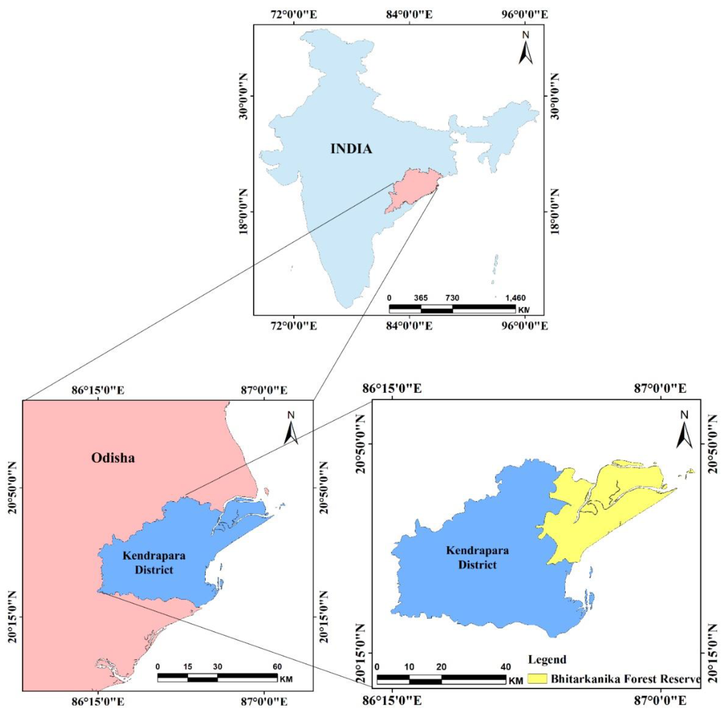
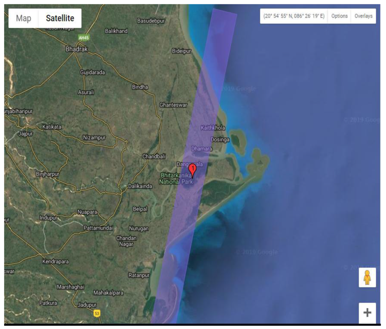
2.1. Study Area

Our study site is located in the Kendrapara district of Odisha, India, which lies between 20°41′36.70″ and 24°45′28″ N latitude and 86°54′17.29″ and 86°92′8.96″ E longitude (as shown in Figure 1). Geographically, it covers an area of around 41.05 Km² of which mostly low-lying (10–25 m above mean sea level) covered with dense mangrove forests. The Bhitarkanika Forest Reserve is a protected forest reserve with a unique habitat and ecosystem. About two-third of the Bhitarkanika Forest Reserve is covered by the Bay of Bengal, and this estuarial region (lies within Bramhani-Baitarni) is a predominant inter tidal zone. Bhitarkanika Forest Reserve is home to a diverse types flora and fauna including some endangered species; it is the second largest mangrove forest in India formed by the estuarial formation of Brahmani-Baitarni, Dhamra, and Mahanadi rivers [67].

The study area comes under the humid sun-tropical climatic region broadly having three seasons namely, summer in which the temperature reaches up to 43 °C, winter in which the temperature goes down to as low as 10 °C, and the rainy season in which this region faces flash floods and frequent cyclones between the months of June to October. The Bhitarkanika Forest Reserve was chosen for the present study because it contains variety of heterogeneous species. In our work, the 10 most dominant mangrove species (as shown in

Table 2. In-situ measurements of different mangrove species in the Bhitarkanika forest reserve.

	Species	Tree Height (m)	Diameter at Breast Height (DBH) (cm)	No of Trees	Wood Density (g/cm3)	Stem volume (m3)	Biomass (t. ha1)	Carbon stock (t. C ha1)
1	Excoecaria agallocha L.	18.45 ± 2.11	20.14 ± 2.56	11	0.49	6.46	222.74 ± 11.17	104.68 ± 5.24
2	Cynometra iripa Kostel	17.23 ± 1.62	16.54 ± 4.39	10	0.81	3.70	231.43 ± 29.09	108.77 ± 13.67
3	Aegiceras corniculatum (L.)	15.03 ± 1.82	22.17 ± 2.81	9	0.59	5.22	262.44 ± 13.84	123.34 ± 6.50
4	Heritiera littoralis Dryand ex Ait.	18.17 ± 2.17	17.21 ± 2.56	10	1.06	4.22	339.13 ± 23.85	159.39 ± 11.21
5	Heritiera fomes Buch.-Ham.	12.35 ± 1.03	18.83 ± 2.94	12	0.88	4.13	287.66 ± 12.81	135.20 ± 6.02
6	Xylocarpus granatum Koenig	14.13 ± 2.01	27.52 ± 4.28	5	0.67	4.20	379.64 ± 38.10	178.43 ± 17.90
7	Xylocarpus mekongensis Pierre	15.38 ± 1.98	20.28 ± 3.40	8	0.73	3.97	162.13 ± 26.30	76.20 ± 12.36
8	Intsia bijuga (Colebr.) Kuntze	12.29 ± 1.38	26.69 ± 4.90	9	0.84	6.18	196.92 ± 32.78	92.55 ± 15.40
9	Cerbera odollam Gaertn.	12.24 ± 1.86	28.56 ± 5.05	6	0.33	4.70	355.36 ± 24.69	167.01 ± 11.60
10	Sonneratia apetala Buch.-Ham.	11.25 ± 1.67	21.85 ± 4.06	10	0.53	4.22	351.14 ± 23.14	165.03 ± 10.87
	Average						278.86 ± 23.57	131.06 ± 11.08

) were identified and used for further analysis.

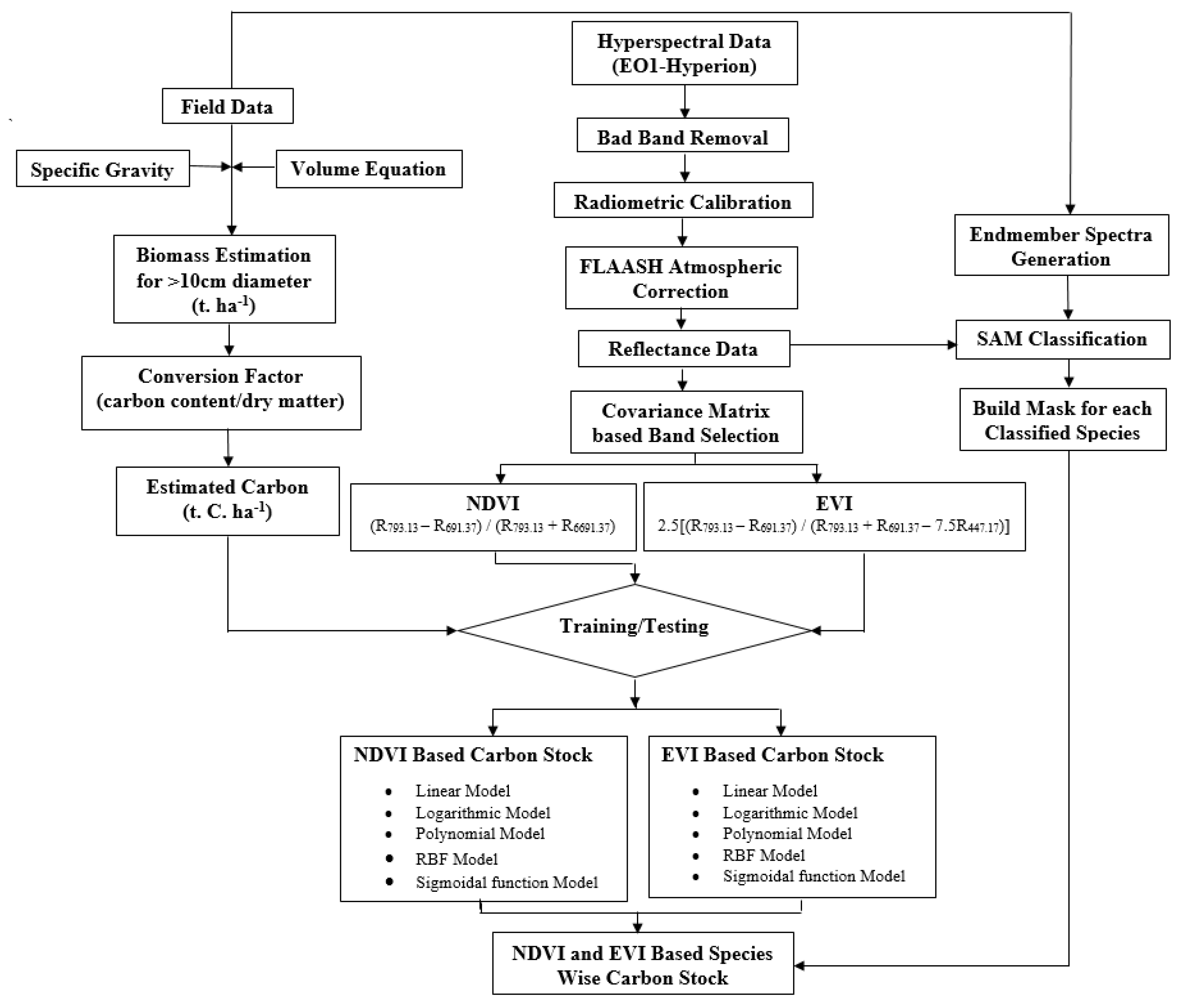
2.2. EO Data Acquisition

EO-Hyperion images (L1Gst) were obtained over the study area from the United States Geological Survey (USGS). The specifications of Hyperion sensor are illustrated in

Table 3. Hyperion Data Description

Satellite Data	EO-Hyperion
Path/Row	139/45
Spatial Resolution	30 meters
Flight Date	31 December 2015
Inclination	97.97 degree
Cloud Cover	<5%

. Hyperion has a spatial resolution of 30 m and 242 spectral bands covering 356 nm to 2577 nm wavelengths. The Hyperion data strip passing over Bhitarkanika Forest Reserve is shown in Figure 2. Out of the 242 spectral bands, 46 bands are considered as bad bands (including 1–7, 58–78, 120–132, 165–182, 185–187, and 221–242 bands), and thus, these were not considered in further analysis. Bad bands have a high amount of noise caused by the water absorption in atmosphere, band overlaps, and lack of proper illumination. The performed image pre-processing includes noise removal and cross track illumination correction. In addition, atmospheric correction has been applied to remove atmospheric noises using the FLAASH (Fast Line-of-sight Atmospheric Analysis of Hyper Spectral-cubes) module in ENVI (v. 5.2) software [68]. After completing this step, endmember extraction was performed for each of the targeted species using the final Hyperion reflectance image and the in-situ GPS (Global Positioning System) locations.

2.3. Field-Inventory Based Biomass Measurement

Field sampling was undertaken during 2015 for the study site. The foremost steps are the prior knowledge of the mangrove plant species; their location and its structure were essential for collecting the sample data for geospatial analysis. Random and the most homogenous patches within the Bhitarkanika Forest Reserve were selected for the field survey to measure tree height, number of samples (trees), Diameter at Breast Height (DBH), and total number of species within the plot.

As the study site selected is 36.42 km² falling within the range of Hyperion data strip (Figure 2). Hyperion image has limited coverage over the Bhitarkanika forest range, and for this reason, a region was selected that falls within the area covered by the Hyperion field of view. The samples were collected by making a 90 × 90 m² grid and it is further divided into nine equal 30 × 30 m² sub-grids, i.e., 90 sub-grids were examined. The most homogenous grid was taken into consideration. This process was then repeated to identify the 10 most homogenous mangrove plant species within the study area and samples were collected using GPS and Clinometer. The field data records the vegetation parameters using GPS in multiple directions. The number of tree species was counted within the plot in random sampling design in the Bhitarkanika Forest Reserve [69]. An overview of the methodology implemented is available in Figure 3. These major species were identified for the study site and their spectral profile was extracted using EO-1 Hyperion dataset. Total area covered by these species was 36.42 km² (see Figure 2). Non-vegetative regions were masked out from the study region.

The Spectral Angle Mapper (SAM) supervised classification algorithm was used for the land use/cover classification using ENVI software [70,71]. SAM is a physically-based spectral classification algorithm, according to [72] that calculates the spectral similarity between a pixel spectrum and a reference spectrum as “the angle between their vectors in a space with dimensionality equal to the number of bands” [72]. SAM uses the calibrated reflectance data for classification and thus relatively insensitive to illumination and albedo effects. End-member reference spectra used in SAM were collected directly from acquired hyperspectral images. SAM compares the angle between reference spectrum and each pixel of an image in n-D space [72,73,74]. This ‘spectral angle’ (α) is calculated as:

$$\mathsf{\alpha } = {\cos }^{-1} \frac{\left( \mathrm{t}.\mathrm{r} \right)}{\left( \Vert \mathrm{t}\Vert \Vert \mathrm{r}\Vert \right)}$$

(1)

where α is the angle between reference spectra and endmember spectra, t is the endmember spectra, and r is the reference spectra.

A thorough and detailed investigation was performed to develop a criterion to estimate different species and determine variety of communities present in that ecosystem. To perform the sampling, firstly, the area is sub-divided into homogeneous patches or units, and furthermore, the samples were taken within these homogenous patches. The total number of transect sampling units to determine the allowable error was calculated using (Chacko, 1965) as follows:

$$\mathrm{N}=\frac{\mathrm{t}{\left(\mathrm{CV}\right)}^2}{{\mathrm{E}}^2}.$$

(2)

where N is the total number of samples, t is the Student’s (t-statistics) value at a 95% significance level, CV is the coefficient of variation (in %), and E is the confidence interval (in mean %).

While performing the field sampling, a transect of 30 m × 30 m plot was laid on the most dominant patch for each species inside the protected area of Bhitarkanika forest reserve. The collected field sampling points were further distributed, and 2/3 of the samples were used for generating the models, whereas 1/3 of the samples were used for validation purpose. Table 2 has shown the field measurements of each species, e.g., scientific name, tree height, DBH, total number of trees within the sample plot, wood density of each species, biomass, and carbon stock. The trees whose girth height was below 1.32 m and DBH < 10 cm were not taken under consideration. The geographical location (latitude and longitude) was recorded using hand-held GPS. There were several mathematical equations developed and used by researchers for biomass estimation of trees [75,76,77,78,79,80,81]. These equations are species specific, particularly in the tropics. The general equation has been developed in modified form. It is more general in nature ([78,82,83]) and applicable in field. It is not possible to cut all the trees to estimate their biomass. Considering the mathematical terms, the models were developed by [76,77,83,84]. The model developed by [75] (1989) to estimate above ground biomass has been used in the present investigation. The literature revealed that this method is non-destructive and is the most suitable method. The biomass for each tree is calculated using the following allometric equation [76,83,85]:

$$\mathrm{Y}=\exp \left[-2.4090+0.9522 \ln \left({\mathrm{D}}^2\times \mathrm{H} \times \mathrm{S}\right)\right].$$

(3)

where Y is above ground biomass (t. ha¹), D is the diameter at breast height, H is the tree height, and S is the wood density. The average wood density (S) for each species is taken from the wood density database provided by the International Council for Research in Agroforestry (ICRAF). From the acquired wood density, it was found that the wood density of Cerbera odollam Gaertn. was lowest (0.3349 gcm³), followed by Excoecaria agallocha L. (0.49 gcm³) among all. Heritiera littoralis Dryland ex Ait. had the highest (0.848 gcm³) wood density. The above ground carbon was calculated using the following formula to estimate biomass [83,85,86]:

Y = B ∗ 0.47

(4)

where Y is the above ground carbon stock (t. ha¹) and B is the above ground biomass per hectare (t. C ha¹).

The precise location of the in-situ ground control points of each species were further used to generate the spectral profile using Hyperion hyperspectral data as shown in Figure 4. The generated spectra of each species were given as an input to the SAM classifier. It is observed that Intsia bijuga (Colebr.) Kuntze is showing the highest reflectance among other observed species, whereas Aegiceras corniculatum (L.) has the lowest reflectance.

2.4. Covariance Matrix Based Band Selection

Hyperspectral data are a set of hundreds of narrow bands at different wavelengths posing problems related to computational complexity, high data volume, bad bands, etc. Therefore, dimensionality reduction of hyperspectral data is considered as one of the solutions for the aforementioned issue. The dimensionality reduction technique is further classified into two groups, namely, feature extraction and feature selection. In the present study, an approach has been made to select the best band for calculation of different vegetation indices. Band selection generally involves two major steps, which are selection of criterion function and optimum band searching. The selection criterion applied in this study is the one proposed by [87], which was named Maximum ellipsoid volume criterion (MEV).

Mathematically it can be formulated as:

$$\mathrm{J}\left(\mathrm{s}\right)=\det \left(\frac{1}{\mathrm{M} - 1}\right){\mathrm{S}}^{\mathrm{T}}\mathrm{S}$$

where M is the number of pixels and S is the selected bands with S = [x₁, x₂, …, x_n] and S^T is the column vector with S^T = [x₁, x₂, …, x_m]^T. Here, n and m are the number of bands and m is the number of number of pixels.

Additionally, for the band searching purpose, sequential forward search was implemented, which basically works on the principle of “down to top”. Here, the first band is defined as the band with maximum variance and the remaining band is compared one by one. While selecting the optimum band, the constant value $\left(\frac{1}{\mathrm{M} - 1}\right)$. is neglected. Thus, Equation (4) can also be written as:

$${\mathrm{B}}_{\mathrm{k}}={\mathrm{S}}_{\mathrm{k}}^{\mathrm{T}}{\mathrm{S}}_{\mathrm{k}}$$

(5)

where B_k is the covariance matrix and S_k = [x₁, x₂, …, x_k]. Therefore, we have:

$${\mathrm{B}}_{\mathrm{k}}={\mathrm{S}}_{\mathrm{k}}^{\mathrm{T}}{\mathrm{S}}_{\mathrm{k}}$$

(6)

= [x₁, x₂, …, x_k]^T [x₁, x₂, …, x_k]

$$= \left[\begin{array}{c}{\mathrm{x}}_1^{\mathrm{T}}{\mathrm{x}}_1 {\mathrm{x}}_1^{\mathrm{T}}{\mathrm{x}}_2 \dots {\mathrm{x}}_1^{\mathrm{T}}{\mathrm{x}}_{\mathrm{k}}\\ {\mathrm{x}}_2^{\mathrm{T}}{\mathrm{x}}_1 {\mathrm{x}}_2^{\mathrm{T}}{\mathrm{x}}_2 \dots {\mathrm{x}}_2^{\mathrm{T}}{\mathrm{x}}_{\mathrm{k}}\\ \dots \dots \dots \dots \\ {\mathrm{x}}_{\mathrm{k}}^{\mathrm{T}}{\mathrm{x}}_1 {\mathrm{x}}_{\mathrm{k}}^{\mathrm{T}}{\mathrm{x}}_2 \dots {\mathrm{x}}_{\mathrm{k}}^{\mathrm{T}}{\mathrm{x}}_{\mathrm{k}}\end{array}\right]$$

According to the rule of determination, the relation between B_k and B_k+1 is described as:

$$\det ({\mathrm{B}}_{\mathrm{k}+1})=\det \left({\mathrm{B}}_{\mathrm{k}}\right)\left({\mathrm{a}}_{\mathrm{k}}-{ \mathrm{d}}_{\mathrm{k}}^{\mathrm{T}}{\mathrm{B}}_{\mathrm{k}}^{-1}{\mathrm{d}}_{\mathrm{k}}\right)$$

(7)

Equation (7) was further used for determining the optimum band; the band that maximizes the value of $\det ({\mathrm{B}}_{\mathrm{k}+1})$ was termed as the optimum band. This band selection method was applied at blue, red, and near infrared bands to further calculate the NDVI and EVI indices.

2.5. NDVI and EVI

In our study, the vegetation indices of NDVI and EVI were employed, which were computed from the Hyperion hyperspectral data to assess the total above ground carbon stock using different allometric regression models [26]. The covariance matrix based band selection algorithm as per described in Section 2.4 determines the specific band for the calculation of vegetation indices. It was observed that the optimum band in NIR (Near-Infrared) region is R_793.13 (surface reflectance at 793.13 nm), in Red region, it is R_691.37 (surface reflectance at 691.37 nm), and in Blue region the optimum band is observed at R_447.17 (surface reflectance at 447.17 nm). The NIR and Red bands were used to calculate the NDVI; as shown in Equation (5), its value ranges from −1 to +1. The negative NDVI values shows waterbody and bare soil, whereas positive values are the green vegetation. The higher the NDVI value, the higher will the density of forest or vegetation be because of the high NIR reflectance and low Red reflectance coming from dense vegetation [88,89]. NDVI has been widely used to monitor vegetation health, density, changes, amount and condition of vegetation:

$$\mathrm{NDVI}= \frac{\left({\mathrm{R}}_{793.13}-{\mathrm{R}}_{691.37}\right)}{\left({\mathrm{R}}_{793.13}+{\mathrm{R}}_{691.37}\right)}$$

(8)

EVI (Enhanced Vegetation Index) was originally developed as an improvement over NDVI; EVI is basically an optimized vegetation index that is used to enhance the sensitivity of high biomass region and it decouples the background variables as well as the atmospheric influences [90,91]. EVI is calculated as follows:

$$\mathrm{EVI}=2.5\ast \frac{\left({\mathrm{R}}_{793.13}-{\mathrm{R}}_{691.37}\right)}{\left({\mathrm{R}}_{793.13}+6{\ast \mathrm{R}}_{691.37}-7.5{\ast \mathrm{R}}_{447.17}+\mathrm{L}\right)}$$

(9)

where L is the adjustment factor, generally 1.

In the present study, both NDVI and EVI were employed to correlate the carbon stock of the Bhitarkanika mangrove forest. EVI is considered as more robust proxy of biomass and carbon stock estimation, as it has better resilience to saturation and resistant to atmospheric contamination and soil [90,92].

Five different models, linear, polynomial, logarithmic, Radial Basis Function (RBF), and sigmoidal function, were utilized for assessing carbon using hyperspectral data derived from NDVI and EVI indices. The relationship of field measured above ground carbon with the NDVI and EVI vegetation indices for all the five models were calculated. The field measured above ground carbon was trained with NDVI and EVI values retrieved from hyperspectral image in each of the five models. The 2/3 of the in-situ measurements were used for training the data, while 1/3 of the remaining data were used for testing the models.

3. Results

This section provides a concise and precise description of the experimental results for blue carbon for a mangrove forest.

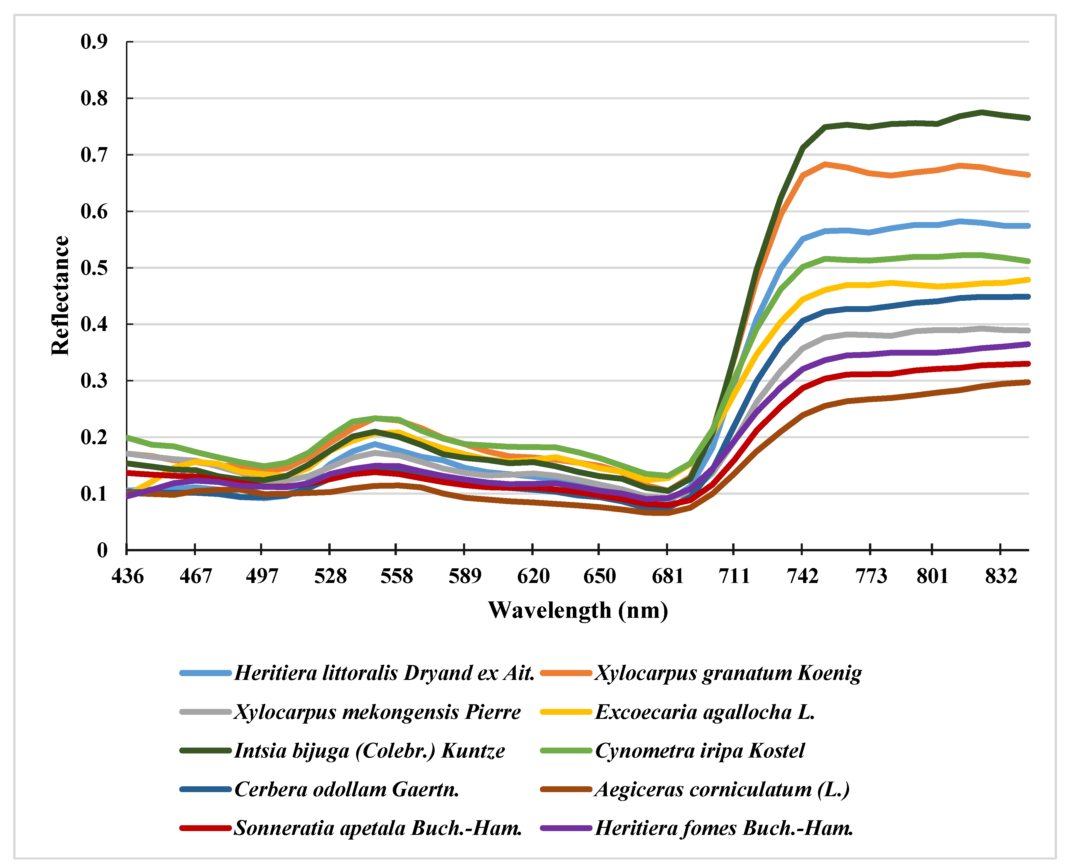
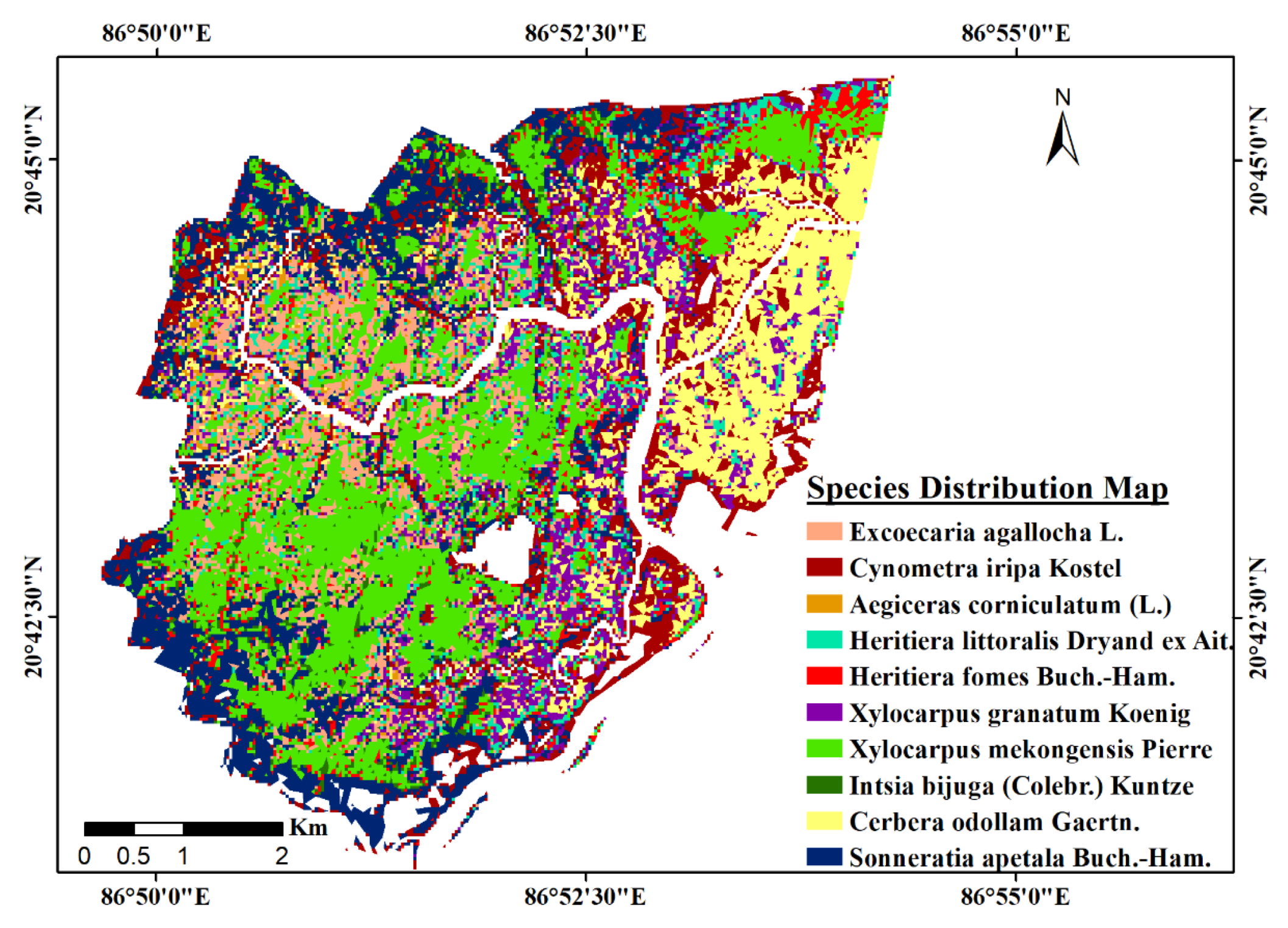
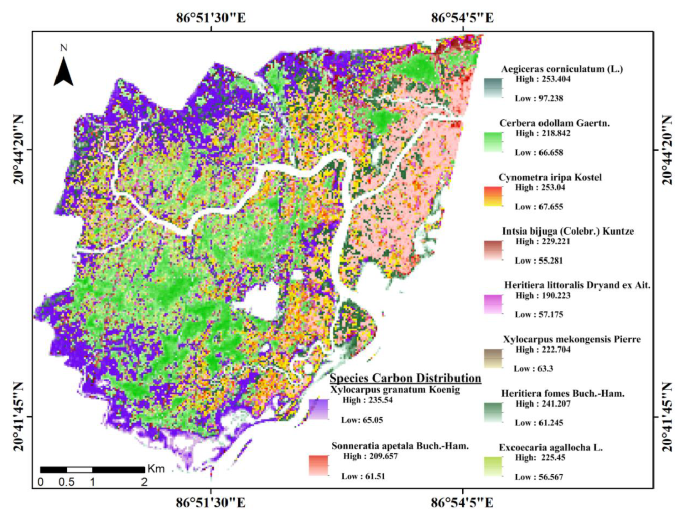
3.1. Spatial Distribution of Species

This section demonstrates the species-wise carbon stock spatial distribution and overall carbon stock of the Bhitarkanika forest reserve and delivers a brief analysis on the overall results. SAM classification (Figure 5) achieved an OA of 84% and a kappa coefficient (k) of 0.81. These results indicate that SAM classification algorithm performed very well in determining the major plant species. These outputs were further taken into account and were used to derive the estimated carbon stock for each species using NDVI and EVI models and illustrating the species-wise carbon stock.

As per

Table 4. (a) Species-wise carbon stock derived from NDVI and (b) EVI for the Bhitarkanika forest reserve.

(a)	Species Name			NDVI Derived Carbon Stocks
		Area (km2)	Total carbon (kt. C)	Min carbon (t. C ha-1)	Max carbon (t. C ha-1)	Ave. carbon ± SD (t. C ha-1)
1	Excoecaria agallocha L.	3.80	52.25	68.14	258.23	143.48 ± 17.39
2	Cynometra iripa Kostel	3.77	42.20	55.28	226.90	115.88 ± 19.61
3	Aegiceras corniculatum (L.)	0.96	54.59	69.66	254.65	149.90 ± 5.57
4	Heritiera littoralis Dryand ex Ait.	2.07	53.08	83.76	225.30	145.55 ± 7.88
5	Heritiera fomes Buch.-Ham.	4.21	51.69	72.47	258.83	141.95 ± 10.60
6	Xylocarpus granatum Koenig	6.41	54.69	55.28	252.01	150.50 ± 15.51
7	Xylocarpus mekongensis Pierre	0.48	47.48	67.35	258.84	130.39 ± 12.70
8	Intsia bijuga (Colebr.) Kuntze	1.66	50.21	83.36	256.40	137.87 ± 12.57
9	Cerbera odollam Gaertn.	8.34	56.36	68.52	219.66	154.78 ± 18.39
10	Sonneratia apetala Buch.-Ham.	4.72	51.84	76.91	254.54	142.34 ±22.46
	Total Area (36.42 km2)	36.42	514.47
(b)	Species Name	EVI Derived Carbon Stocks
		Area (km2)	Total carbon (kt. C)	Min carbon (t. C ha−1)	Max. carbon (t. C ha−1)	Ave. carbon ± SD (t. C ha−1)
1	Excoecaria agallocha L.	3.80	45.22	56.57	225.45	124.18 ± 10.15
2	Cynometra iripa Kostel	3.77	31.02	61.25	241.22	85.19 ± 26.29
3	Aegiceras corniculatum (L.)	0.96	44.35	63.30	222.70	121.80 ± 16.38
4	Heritiera littoralis Dryand ex Ait.	2.07	42.45	57.17	190.22	116.57 ± 22.72
5	Heritiera fomes Buch.-Ham.	4.21	47.38	55.28	229.22	130.11 ± 32.21
6	Xylocarpus granatum Koenig	6.41	46.90	67.66	253.04	128.78 ± 15.70
7	Xylocarpus mekongensis Pierre	0.48	50.60	66.66	218.84	138.95 ± 20.75
8	Intsia bijuga (Colebr.) Kuntze	1.66	53.10	97.24	253.40	145.83 ± 18.84
9	Cerbera odollam Gaertn.	8.34	48.56	61.51	209.66	133.36 ± 10.19
10	Sonneratia apetala Buch.-Ham.	4.72	50.19	61.05	235.54	137.83 ± 15.30
	Total Area (36.42 km2)	36.42	459.82

, it has been observed that the total aboveground carbon from EVI and NDVI derived aboveground carbon are 459.82 kt. C and 514.47 kt. C, respectively. The NDVI derived carbon is showing higher value than the EVI derived carbon because NDVI values can be influenced by the atmospheric contaminants, topography, soil, and dense biomass. These can lead to the increase in the irradiance of the NIR band and result in bias. It should also be noted that NDVI saturates in dense vegetation so that the accuracy of NDVI values differ by land use, topography, and atmospheric conditions [90,93,94,95]. Santin-Janin et al. [96] used non-linear model coupled with NDVI and EVI estimates to estimate the biomass and carbon stock. Wicaksono et al. [97] employed 13 vegetation indices to assess the above ground carbon of mangrove forest and concluded that the best fitted above ground carbon model for mangrove species derived from vegetation indices was EVI1 (R²=0.688), whereas for below ground carbon GEMI (R²=0.567) showed the best fit. Similarly, Adam et al. [95] utilized the narrow band vegetation indices with all possible band combinations using hyperspectral data for above ground biomass and concluded EVI is more robust for the assessment. Different band selections were used by them to enhance the predictive accuracy, the best three combinations for estimating EVI are (a) 445 nm, 682 nm, and 829 nm, (b) 497 nm, 676 nm, and 1091 nm, and (c) 495 nm, 678 nm, and 1120 nm.

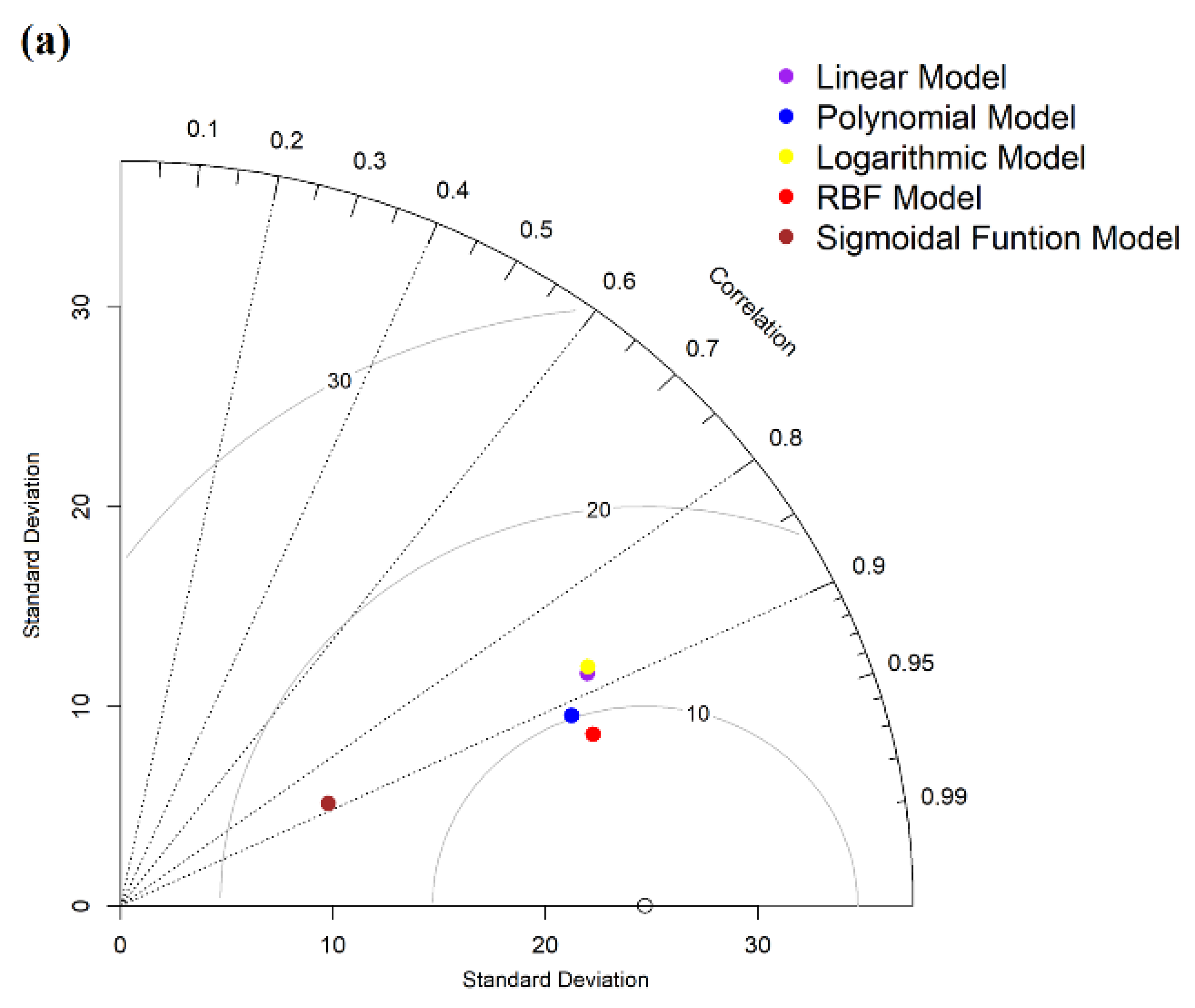
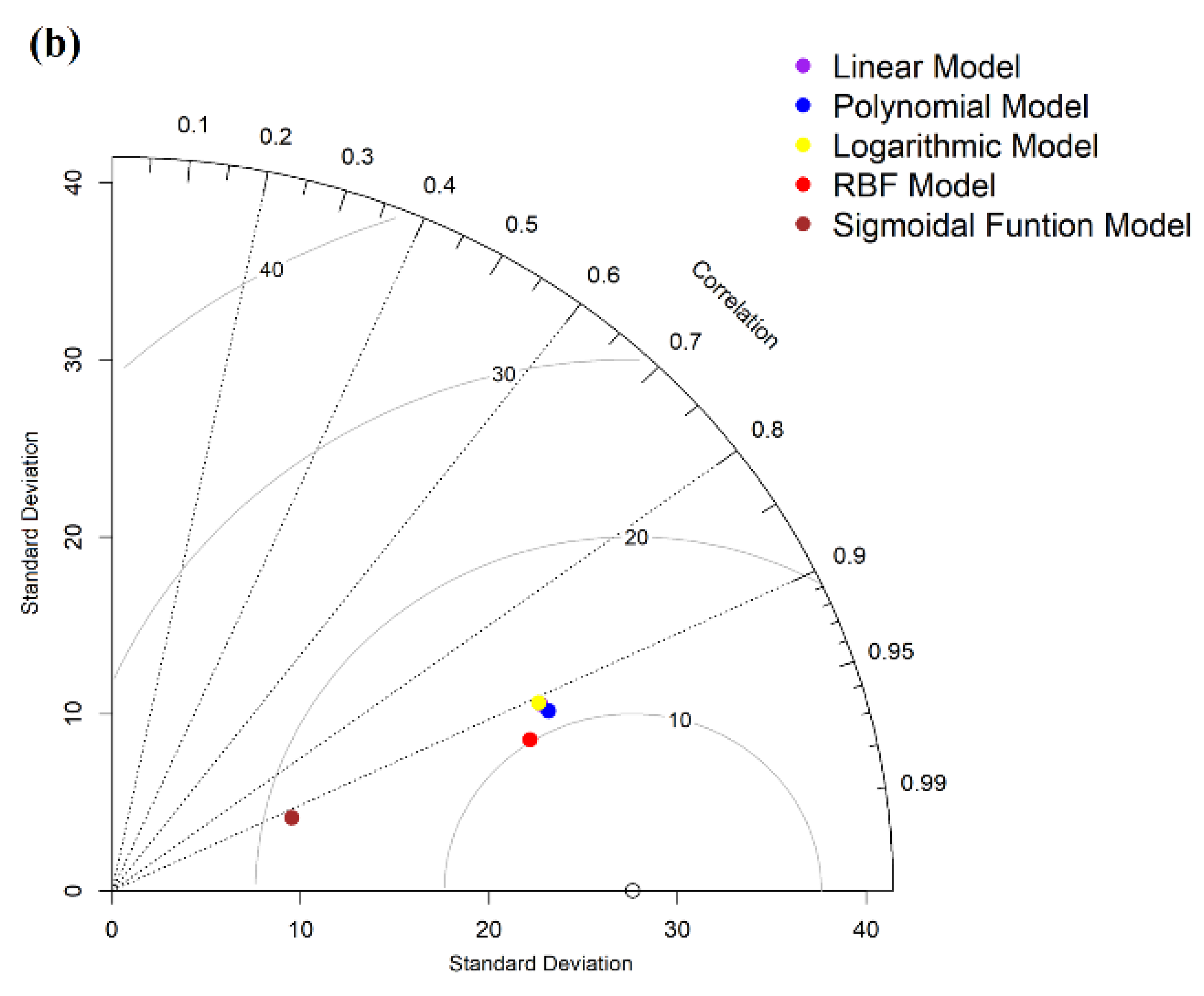
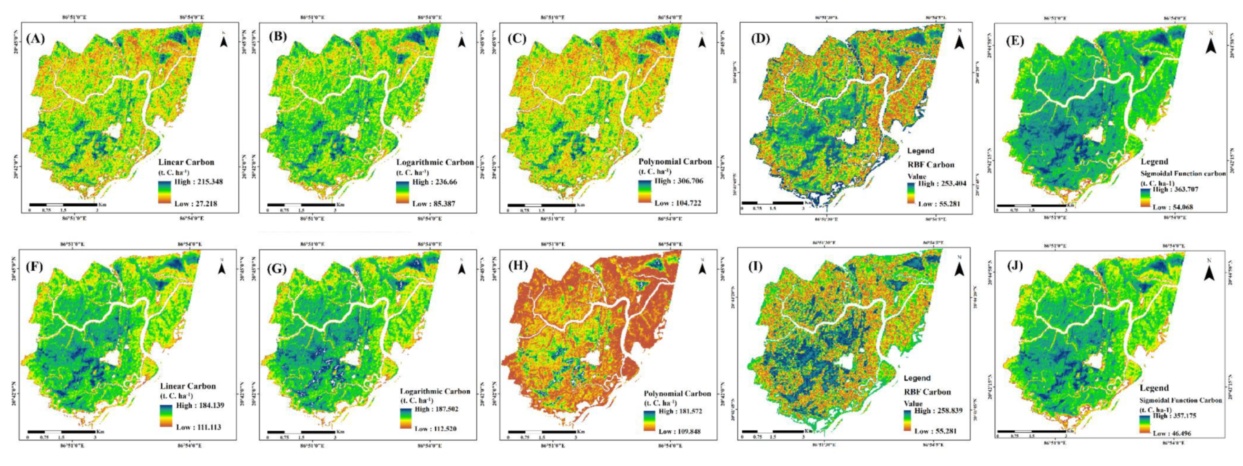
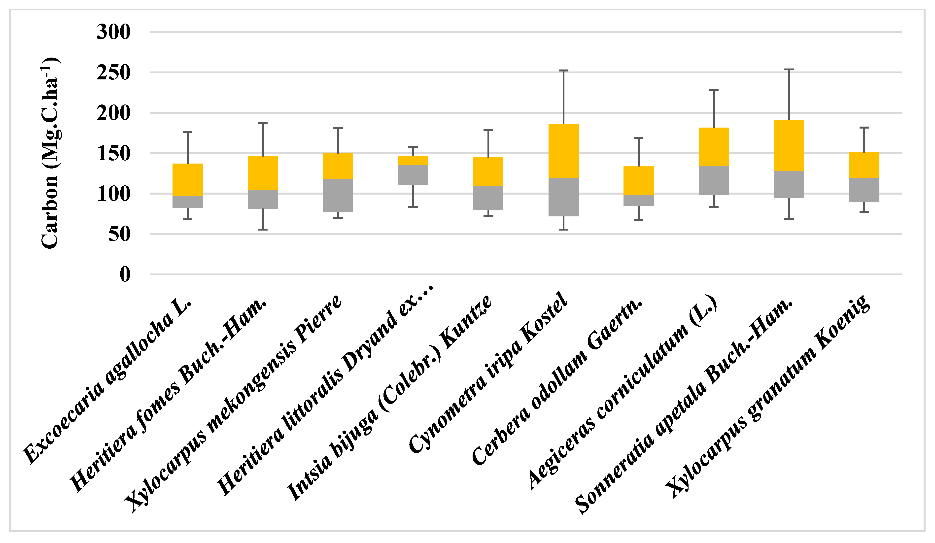
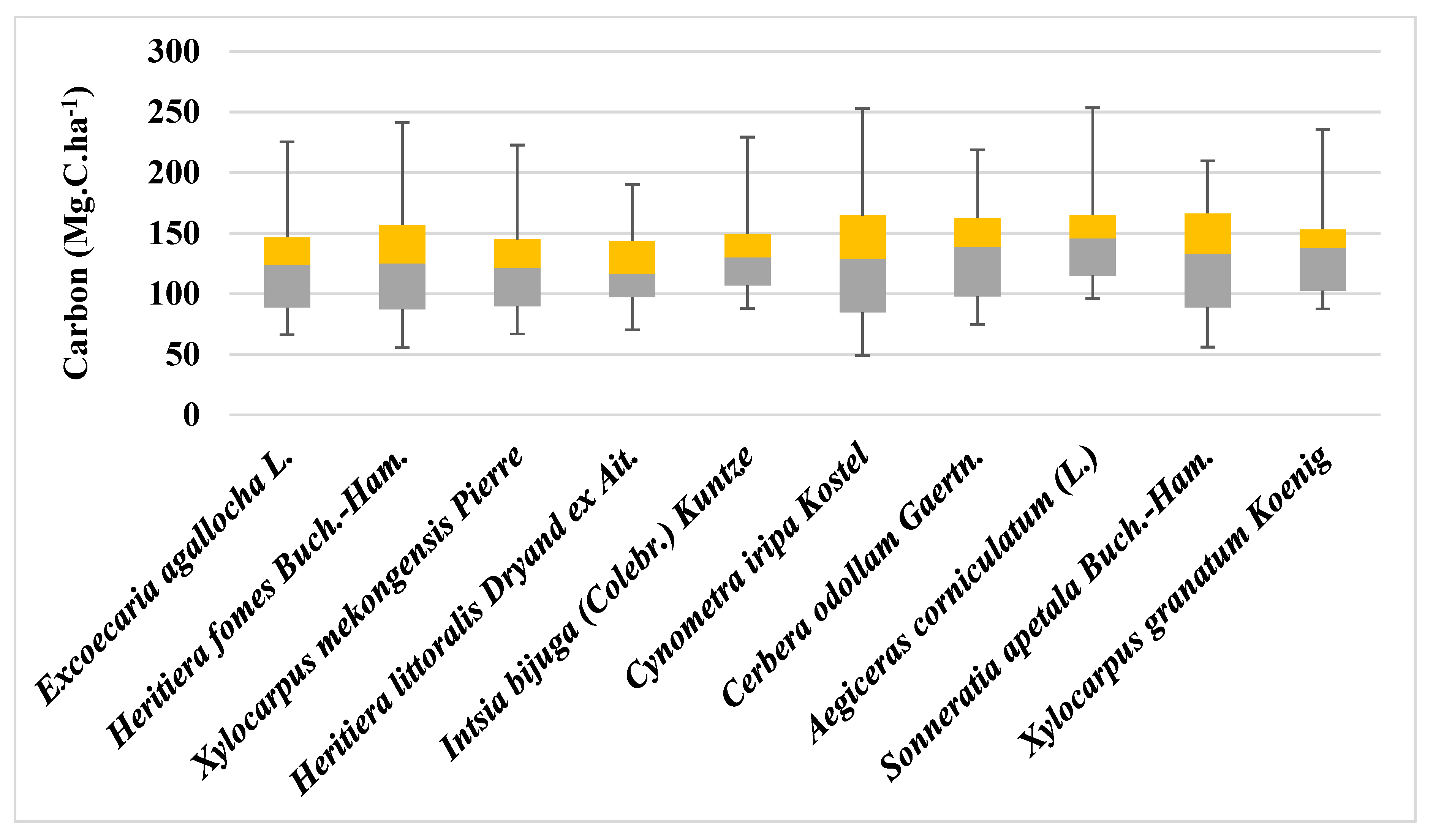
3.2. Estimation of Carbon Stock Using Spectral Derived Indices

This section presents the carbon stock assessment for mangrove forest using different models namely, linear, logarithmic, polynomial (second degree), RBF, and sigmoidal function. All the models were trained with the EVI and NDVI generated relations with the ground measured data as well as tested with the modeled biomass and observed carbon stock as shown in Figure 6. The latter figure illustrates the performance of each model for EVI and NDVI based estimations; it can be observed that the RBF model performed better than the others.

According to the distributed EVI value, it has been concluded that a good amount of area is under dense coverage of forest species; moreover, it has shown higher estimation of carbon stock than NDVI. EVI varies from 0.35 to 6.9 and it is more sensitive to branches and other non-photosynthetic parts of the vegetation (parts different from leaves). EVI is more sensitive to plant parameters, as it avoids the atmospheric effects as well as the soil background. The results illustrate that EVI derived carbon varies from 27.22 to 215.35 t. C ha⁻¹ for linear, 85.39 to 236.66 t. C ha⁻¹ for log, 104.72 to 306.70 t. C ha⁻¹ for polynomial, 55.281 to 253.4 t. C ha⁻¹ for RBF and 54.068 to 363.7 t. C ha⁻¹ for sigmoidal function models (See Figure 7A–E). NDVI derived carbon varies from 111.11 to 184.14 t. C ha⁻¹ for linear, 112.53 to 187.50 t. C ha⁻¹ for log, and 109.85 to 181.57 t. C ha⁻¹ for polynomial, 55.281 to 258.84 t. C ha⁻¹ for RBF, and 46.5 to 357.17 t. C ha⁻¹ for sigmoidal function models (See Figure 7F–J). Estimated carbon is highest for EVI derived sigmoidal function model with highest carbon content up to 363.7 t. C ha⁻¹ and lowest for linear regression models reaching up to only 27.22 t. C ha⁻¹. Lowest estimated carbon for NDVI derived carbon stocks comes to be 46.5 t. C ha⁻¹ for the sigmoidal function model and highest values was observed as 357.17 t. C ha⁻¹ for the sigmoidal function model.

The carbon stock values from the satellite-derived indices fall within the expected ranges for mangrove carbon stocks. NDVI values range from 0.5 to 0.65; the latter shows a healthy, dense mangrove forest in Bhitarkanika. The final interpretation result reveals that the middle northern part of the study area is showing higher biomass values (~250 t. C ha⁻¹). Thus, it is concluded that these regions are highly dense and stores an ample amount of blue carbon in it.

The polynomial regression model using EVI is found to be suitable for the estimation of carbon stock at the study site, with an R² of 0.87. EVI has shown high amount of estimated carbon ranges as it is more sensitive to biomass, and ultimately affecting the carbon estimation as compared to the NDVI and can be seen from Figure 7 and Table 4 whereas, NDVI has shown more consistent outcomes in the case of minimum and maximum estimated carbon stocks.

3.3. Species-Wise Carbon Stock Assessment

The classification results generated from SAM classifier and the covariance matrix based optimum band selection for generating vegetation indices were further used to extract the species-wise carbon stock as well as the area covered by each species in the Bhitarkanika forest reserve (see Figure 8 and Figure 9). Figure 9 illustrates the NDVI derived carbon distribution map for each major species, while Figure 8 demonstrates the EVI derived carbon distribution map for each major species. It is also important to notice that the carbon stock of each species shows some variance, which is investigated and presented in Figure 10 and Figure 11. Furthermore, the outcome of species-wise carbon stocks depends upon the species classification accuracies for species distribution classification maps.

Total area covered by the major mangrove species was around 36.42 km². Cerbera odollam Gaertn covers the largest part of the forest, approximately 22.90% of the total area. Total estimated carbon for the EVI derived indices is 49.82 kt. C. and total carbon estimated for the Bhitarkanika forest derived from NDVI indices is 514.47 kt. C. Using EVI-derived carbon stocks, the highest contribution of carbon stock is the Intsia bijuga (Colebr.) Kuntze species with 53.10 kt. C (11.54%). From the NDVI derived carbon stocks, Cerbera odollam Gaertn seems to contribute the most with 56.36 kt. C (10.95%). Field measured carbon was recorded lowest for the species Xylocarpus mekongensis Pierre, which was 76.20 t. C ha⁻¹. Figure 8 shows the spatial distribution of carbon derived from EVI for each species. Intsia bijuga (Colebr.) Kuntze shows highest carbon content up to 253.4 t. C ha⁻¹. The highest carbon stocks as derived from NDVI were displayed for Xylocarpus mekongensis Pierre at 258.84 t. C ha⁻¹.

As such, while Cerbera odollam Gaertn covers most of the area (22.9%), differences in carbon per hectare (Carbon area density) promote Intsia bijuga (Colebr.) Kuntze as the highest contributing species in the Bhitarkanika forest with EVI-derived carbon stocks. This is due to the large difference between EVI and NDVI derived carbon area density for Cerbera odollam Gaertn (average 128.78 ± 15.702 t. C ha⁻¹ and 150.498 ± 15.51 t. C ha⁻¹). Cross-referencing with the measured values presented in Table 2 (165.03 ± 10.87167.02 t. C ha⁻¹), leads to the conclusion that the NDVI derived carbon stocks for Cerbera odollam Gaertn are more accurate. This conclusion is not reflective of all the species. Out of the 10 species examined, the average Carbon area density of EVI is closer to the measured value in six of them, while NDVI derived Carbon area density is more accurate in the other four. The greatest divergence between EVI and NDVI estimated carbon area densities is for Cerbera odollam Gaertn. Significant differences are also shown for Intsia bijuga (Colebr.) Kuntze and Xylocarpus mekongensis Pierre.

A species-wise box-plot is generated to assess the variation in different species-wise carbon stock estimated using EVI and NDVI, which is shown in Figure 10 and Figure 11, with the minima, maxima, median, 25% quartile, and 75% quartile. The average carbon stock measured from field sampling is 131.07 t. C ha⁻¹. Average EVI derived carbon stock ranges from 77.86 t. C ha⁻¹ to 135.28 t. C ha⁻¹ and for NDVI derived carbon stock 116.57 t. C ha⁻¹ to 145.82 t. C ha⁻¹ for the Bhitarkanika mangrove forest. As such, both EVI and NDVI estimated averages are in agreement with the average carbon stock measured from the field.

4. Conclusions

Mangrove forests store a large quantity of blue carbon in plants, both in the form of biomass and as sediment in the soil. Anthropogenic activities threaten these forests nowadays due to conversion to other land use types. Such transition of forest areas is a major source of carbon emissions to the atmosphere. As such, carbon stock assessment is essential to reduce the loss of biomass in such ecosystems. Species-wise blue carbon analysis can be used to assess the impact of global climate change on different mangrove species as well as to help policy makers to accurately evaluate the ecological and economical trade off associated with the management of mangroves ecosystem. The present study aimed at demonstrating the use of hyperspectral EO data for species identification in a highly diversified mangrove ecosystem and for calculating total carbon stored. The Bhitarkanika forest in India was chosen as a study site and Hyperion hyperspectral images were used.

There have been several studies on the blue carbon stored in mangroves, however, thus far, a species wide blue carbon analysis with significant accuracy was missing. This study attempts to mitigate that gap of knowledge by estimating the above-ground carbon stocks for each of the 10 major species that were identified and found dominant in the study area.

Hyperspectral data from EO-1 Hyperion were collected and processed to extract the biophysical parameters of interest. Near co-orbital field measurements of biomass and carbon measurements were acquired for validation. The in-situ locations of mangrove species were used to generate spectral profile. The spatial distribution of the major mangrove species was identified using the SAM classification algorithm, which performed reliably well (e.g., kappa coefficient κ = 0.81). NDVI and EVI radiometric indices were calculated from the optimum bands, obtained by covariance matrix based band selection algorithm. Several models were tested to relate NDVI and EVI with carbon stocks. The RBF model performed best (R² = 86.98% for EVI and R² = 84.1% for NDVI) and was subsequently used in this study to estimate carbon stocks for the 10 dominant species and the entire study area.

Despite the significance of mangrove ecosystem and blue carbon for local as well as global climate, the drastic transformation of mangrove forests into other land use types is directly affecting the livelihood around it, which can be seen through the shortage of firewood, regular soil erosion, and decrease in fishing zones. Therefore, there should be adequate digital information about the coverage, biomass, and carbon content of the mangrove forest for quick management and planning. The present study provides evidence that NDVI and EVI indices have a very promising potential to be applied in classifying the dominant species of mangrove forests and coastal ecosystems according to their carbon content. These indices can provide adequate estimates of maximum, minimum, and average carbon content for a large area and show the spatial distribution of carbon, and thus, biomass. The above-ground carbon stocks for each species were estimated and presented in this study. For the whole study area, the carbon stocks were estimated 459.82 kt. C. from EVI and 514.47 kt. C. from NDVI.

The only limitation faced in this study was the limited availability of Hyperion data and that too covering a part of Bhitarkanika as shown in Figure 2. Using the same methodology with spectral images from different satellites could provide better coverage, and thus carbon stock estimations of different areas. Future studies could focus on different ecosystems to assess the effectiveness for this method and estimate carbon stock for different areas and ecosystems in order to provide the tools for a better evaluation of biomass and global carbon stocks; this remains to be seen.

References

1. Saenger, P.; Hegerl, E.; Davie, J.D. Global Status of Mangrove Ecosystems; International Union for Conservation of Nature and Natural Resources: Gland, Switzerland, 1983. [Google Scholar]
2. Barbier, E.B. The protective service of mangrove ecosystems: A review of valuation methods. Mar. Pollut. Bull. 2016, 109, 676–681. [Google Scholar] [CrossRef]
3. Houghton, R.; Hall, F.; Goetz, S.J. Importance of biomass in the global carbon cycle. J. Geophys. Res. Biogeosci. 2009, 114. [Google Scholar] [CrossRef]
4. Conservation-International. The Blue Carbon Initiatives. Available online: https://www.thebluecarboninitiative.org/ (accessed on 15 May 2019).
5. Giri, C.; Ochieng, E.; Tieszen, L.L.; Zhu, Z.; Singh, A.; Loveland, T.; Masek, J.; Duke, N. Status and distribution of mangrove forests of the world using earth observation satellite data. Glob. Ecol. Biogeogr. 2011, 20, 154–159. [Google Scholar] [CrossRef]
6. FSI. Mangrove Cover. Available online: http://fsi.nic.in/isfr2017/isfr-mangrove-cover-2017.pdf (accessed on 23 May 2019).
7. Osland, M.J.; Feher, L.C.; Griffith, K.T.; Cavanaugh, K.C.; Enwright, N.M.; Day, R.H.; Stagg, C.L.; Krauss, K.W.; Howard, R.J.; Grace, J.B. Climatic controls on the global distribution, abundance, and species richness of mangrove forests. Ecol. Monogr. 2017, 87, 341–359. [Google Scholar] [CrossRef] [Green Version]
8. Himes-Cornell, A.; Pendleton, L.; Atiyah, P. Valuing ecosystem services from blue forests: A systematic review of the valuation of salt marshes, sea grass beds and mangrove forests. Ecosyst. Serv. 2018, 30, 36–48. [Google Scholar] [CrossRef]
9. Gilman, E.L.; Ellison, J.; Duke, N.C.; Field, C. Threats to mangroves from climate change and adaptation options: A review. Aquat. Bot. 2008, 89, 237–250. [Google Scholar] [CrossRef]
10. Kairo, J.G.; Lang’at, J.K.; Dahdouh-Guebas, F.; Bosire, J.; Karachi, M. Structural development and productivity of replanted mangrove plantations in Kenya. For. Ecol. Manag. 2008, 255, 2670–2677. [Google Scholar] [CrossRef]
11. Bosire, J.O.; Dahdouh-Guebas, F.; Walton, M.; Crona, B.I.; Lewis, R., III; Field, C.; Kairo, J.G.; Koedam, N. Functionality of restored mangroves: A review. Aquat. Bot. 2008, 89, 251–259. [Google Scholar] [CrossRef] [Green Version]
12. Duke, N.C.; Meynecke, J.-O.; Dittmann, S.; Ellison, A.M.; Anger, K.; Berger, U.; Cannicci, S.; Diele, K.; Ewel, K.C.; Field, C.D. A world without mangroves? Science 2007, 317, 41–42. [Google Scholar] [CrossRef] [Green Version]
13. Hamilton, S.E.; Casey, D. Creation of a high spatio-temporal resolution global database of continuous mangrove forest cover for the 21st century (CGMFC-21). Glob. Ecol. Biogeogr. 2016, 25, 729–738. [Google Scholar] [CrossRef]
14. Hamilton, S.E.; Friess, D.A. Global carbon stocks and potential emissions due to mangrove deforestation from 2000 to 2012. Nat. Clim. Chang. 2018, 8, 240. [Google Scholar] [CrossRef] [Green Version]
15. Valiela, I.; Bowen, J.L.; York, J.K. Mangrove Forests: One of the World’s Threatened Major Tropical Environments. Bioscience 2001, 51, 807–815. [Google Scholar] [CrossRef] [Green Version]
16. Alongi, D.M. Present state and future of the world’s mangrove forests. Environ. Conserv. 2002, 29, 331–349. [Google Scholar] [CrossRef] [Green Version]
17. Allen, J.A.; Ewel, K.C.; Jack, J. Patterns of natural and anthropogenic disturbance of the mangroves on the Pacific Island of Kosrae. Wetl. Ecol. Manag. 2001, 9, 291–301. [Google Scholar] [CrossRef]
18. Giri, C.; Zhu, Z.; Tieszen, L.; Singh, A.; Gillette, S.; Kelmelis, J. Mangrove forest distributions and dynamics (1975–2005) of the tsunami-affected region of Asia. J. Biogeogr. 2008, 35, 519–528. [Google Scholar] [CrossRef]
19. Baillie, J.E.; Hilton-Taylor, C.; Stuart, S.N. A Global Species Assessment; International Union for Conservation of Nature (IUCN): Gland, Switzerland, 2004. [Google Scholar]
20. Kathiresan, K.; Rajendran, N. Mangrove ecosystems of the Indian Ocean region. Indian J. Mar. Sci. 2005, 34, 104–113. [Google Scholar]
21. Sandilyan, S.; Kathiresan, K. Mangrove conservation: A global perspective. Biodivers. Conserv. 2012, 21, 3523–3542. [Google Scholar] [CrossRef]
22. Shanker, K. Biodiversity of Mangrove Ecosystems; Medknow Publications: Mumbai, India, 2005. [Google Scholar]
23. Kathiresan, K.; Qasim, S.Z. Biodiversity of Mangrove Ecosystems; Hindustan Publishing: New Delhi, India, 2005. [Google Scholar]
24. Kathiresan, K. Importance of mangrove forest of India. J. Coast. Environ. 2010, 1, 11–26. [Google Scholar]
25. Kathiresan, K. Why are mangroves degrading? Curr. Sci. 2002, 83, 1246–1249. [Google Scholar]
26. Pandey, P.C.; Anand, A.; Srivastava, P.K. Spatial Distribution of Mangrove Forest species and Biomass Assessment Using Field Inventory and Earth Observation Hyperspectral data. Biodivers. Conserv. 2019, 28, 2143–2162. [Google Scholar] [CrossRef]
27. Yang, C.; Liu, J.; Zhang, Z.; Zhang, Z. Estimation of the carbon stock of tropical forest vegetation by using remote sensing and GIS. In Proceedings of the IGARSS 2001. Scanning the Present and Resolving the Future. In Proceedings of the IEEE 2001 International Geoscience and Remote Sensing Symposium (Cat. No. 01CH37217), Sydney, Australia, 9–13 July 2001; pp. 1672–1674. [Google Scholar]
28. Ramankutty, N.; Gibbs, H.K.; Achard, F.; Defries, R.; Foley, J.A.; Houghton, R. Challenges to estimating carbon emissions from tropical deforestation. Glob. Chang. Biol. 2007, 13, 51–66. [Google Scholar] [CrossRef]
29. Atmadja, S.; Verchot, L. A review of the state of research, policies and strategies in addressing leakage from reducing emissions from deforestation and forest degradation (REDD+). Mitig. Adapt. Strateg. Glob. Chang. 2012, 17, 311–336. [Google Scholar] [CrossRef]
30. Minang, P.A.; Van Noordwijk, M. Design challenges for achieving reduced emissions from deforestation and forest degradation through conservation: Leveraging multiple paradigms at the tropical forest margins. Land Use Policy 2013, 31, 61–70. [Google Scholar] [CrossRef]
31. CIFOR. Global Comparative Study on REDD+ Subnational REDD+ Initiatives. Available online: https://www.cifor.org/gcs/modules/redd-subnationalinitiatives/ (accessed on 25 May 2018).
32. Atwood, T.B.; Connolly, R.M.; Almahasheer, H.; Carnell, P.E.; Duarte, C.M.; Lewis, C.J.E.; Irigoien, X.; Kelleway, J.J.; Lavery, P.S.; Macreadie, P.I. Global patterns in mangrove soil carbon stocks and losses. Nat. Clim. Chang. 2017, 7, 523. [Google Scholar] [CrossRef]
33. Heumann, B.W. An object-based classification of mangroves using a hybrid decision tree—Support vector machine approach. Remote Sens. 2011, 3, 2440–2460. [Google Scholar] [CrossRef] [Green Version]
34. Chaube, N.R.; Lele, N.; Misra, A.; Murthy, T.; Manna, S.; Hazra, S.; Panda, M.; Samal, R. Mangrove species discrimination and health assessment using AVIRIS-NG hyperspectral data. Curr. Sci. 2019, 116, 1136. [Google Scholar] [CrossRef]
35. Kumar, T.; Panigrahy, S.; Kumar, P.; Parihar, J.S. Classification of floristic composition of mangrove forests using hyperspectral data: Case study of Bhitarkanika National Park, India. J. Coast. Conserv. 2013, 17, 121–132. [Google Scholar] [CrossRef]
36. Ashokkumar, L.; Shanmugam, S. Hyperspectral band selection and classification of Hyperion image of Bhitarkanika mangrove ecosystem, eastern India. Proc. SPIE 2014, 9239, 923914. [Google Scholar]
37. Padma, S.; Sanjeevi, S. Jeffries Matusita-Spectral Angle Mapper (JM-SAM) spectral matching for species level mapping at Bhitarkanika, Muthupet and Pichavaram mangroves. Int. Arch. Photogramm. Remote Sens. Spat. Inf. Sci. 2014, 40, 1403. [Google Scholar] [CrossRef] [Green Version]
38. Everitt, J.; Yang, C.; Judd, F.; Summy, K. Use of archive aerial photography for monitoring black mangrove populations. J. Coast. Res. 2010, 26, 649–653. [Google Scholar] [CrossRef]
39. Lam-Dao, N.; Pham-Bach, V.; Nguyen-Thanh, M.; Pham-Thi, M.-T.; Hoang-Phi, P. Change detection of land use and riverbank in Mekong Delta, Vietnam using time series remotely sensed data. J. Resour. Ecol. 2011, 2, 370–375. [Google Scholar]
40. Satyanarayana, B.; Mohamad, K.A.; Idris, I.F.; Husain, M.-L.; Dahdouh-Guebas, F. Assessment of mangrove vegetation based on remote sensing and ground-truth measurements at Tumpat, Kelantan Delta, East Coast of Peninsular Malaysia. Int. J. Remote Sens. 2011, 32, 1635–1650. [Google Scholar] [CrossRef]
41. Pattanaik, C.; Prasad, S.N. Assessment of aquaculture impact on mangroves of Mahanadi delta (Orissa), East coast of India using remote sensing and GIS. Ocean Coast. Manag. 2011, 54, 789–795. [Google Scholar] [CrossRef]
42. Rahman, A.F.; Dragoni, D.; Didan, K.; Barreto-Munoz, A.; Hutabarat, J.A. Detecting large scale conversion of mangroves to aquaculture with change point and mixed-pixel analyses of high-fidelity MODIS data. Remote Sens. Environ. 2013, 130, 96–107. [Google Scholar] [CrossRef]
43. Pu, R.; Bell, S. A protocol for improving mapping and assessing of seagrass abundance along the West Central Coast of Florida using Landsat TM and EO-1 ALI/Hyperion images. ISPRS J. Photogramm. Remote Sens. 2013, 83, 116–129. [Google Scholar] [CrossRef]
44. Lucas, R.; Rebelo, L.-M.; Fatoyinbo, L.; Rosenqvist, A.; Itoh, T.; Shimada, M.; Simard, M.; Souza-Filho, P.W.; Thomas, N.; Trettin, C. Contribution of L-band SAR to systematic global mangrove monitoring. Mar. Freshw. Res. 2014, 65, 589–603. [Google Scholar] [CrossRef]
45. Vu, T.D.; Takeuchi, W.; Van, N.A. Carbon stock calculating and forest change assessment toward REDD+ activities for the mangrove forest in Vietnam. Trans. Jpn. Soc. Aeronaut. Space Sci. Aerosp. Technol. Jpn. 2014, 12. [Google Scholar] [CrossRef]
46. Thomas, N.; Lucas, R.; Itoh, T.; Simard, M.; Fatoyinbo, L.; Bunting, P.; Rosenqvist, A. An approach to monitoring mangrove extents through time-series comparison of JERS-1 SAR and ALOS PALSAR data. Wetl. Ecol. Manag. 2015, 23, 3–17. [Google Scholar] [CrossRef]
47. Garcia, R.; Hedley, J.; Tin, H.; Fearns, P. A method to analyze the potential of optical remote sensing for benthic habitat mapping. Remote Sens. 2015, 7, 13157–13189. [Google Scholar] [CrossRef] [Green Version]
48. Son, N.T.; Thanh, B.X.; Da, C.T. Monitoring mangrove forest changes from multi-temporal Landsat data in Can Gio Biosphere Reserve, Vietnam. Wetlands 2016, 36, 565–576. [Google Scholar] [CrossRef]
49. Nardin, W.; Locatelli, S.; Pasquarella, V.; Rulli, M.C.; Woodcock, C.E.; Fagherazzi, S. Dynamics of a fringe mangrove forest detected by Landsat images in the Mekong River Delta, Vietnam. Earth Surf. Process. Landf. 2016, 41, 2024–2037. [Google Scholar] [CrossRef]
50. Viennois, G.; Proisy, C.; Feret, J.-B.; Prosperi, J.; Sidik, F.; Rahmania, R.; Longépé, N.; Germain, O.; Gaspar, P. Multitemporal analysis of high-spatial-resolution optical satellite imagery for mangrove species mapping in Bali, Indonesia. IEEE J. Sel. Top. Appl. Earth Obs. Remote Sens. 2016, 9, 3680–3686. [Google Scholar] [CrossRef]
51. Pham, L.T.; Brabyn, L. Monitoring mangrove biomass change in Vietnam using SPOT images and an object-based approach combined with machine learning algorithms. ISPRS J. Photogramm. Remote Sens. 2017, 128, 86–97. [Google Scholar] [CrossRef]
52. Benson, L.; Glass, L.; Jones, T.; Ravaoarinorotsihoarana, L.; Rakotomahazo, C. Mangrove carbon stocks and ecosystem cover dynamics in southwest Madagascar and the implications for local management. Forests 2017, 8, 190. [Google Scholar] [CrossRef] [Green Version]
53. Bullock, E.L.; Fagherazzi, S.; Nardin, W.; Vo-Luong, P.; Nguyen, P.; Woodcock, C.E. Temporal patterns in species zonation in a mangrove forest in the Mekong Delta, Vietnam, using a time series of Landsat imagery. Cont. Shelf Res. 2017, 147, 144–154. [Google Scholar] [CrossRef]
54. Mondal, P.; Trzaska, S.; de Sherbinin, A. Landsat-derived estimates of mangrove extents in the sierra leone coastal landscape complex during 1990–2016. Sensors 2018, 18, 12. [Google Scholar] [CrossRef] [Green Version]
55. Wang, M.; Cao, W.; Guan, Q.; Wu, G.; Wang, F. Assessing changes of mangrove forest in a coastal region of southeast China using multi-temporal satellite images. Estuar. Coast. Shelf Sci. 2018, 207, 283–292. [Google Scholar] [CrossRef]
56. Abdel-Hamid, A.; Dubovyk, O.; Abou El-Magd, I.; Menz, G. Mapping Mangroves Extents on the Red Sea Coastline in Egypt using Polarimetric SAR and High Resolution Optical Remote Sensing Data. Sustainability 2018, 10, 646. [Google Scholar] [CrossRef] [Green Version]
57. Pan, Z.; Glennie, C.; Fernandez-Diaz, J.C.; Starek, M. Comparison of bathymetry and seagrass mapping with hyperspectral imagery and airborne bathymetric lidar in a shallow estuarine environment. Int. J. Remote Sens. 2016, 37, 516–536. [Google Scholar] [CrossRef]
58. Warfield, A.D.; Leon, J.X. Estimating Mangrove Forest Volume Using Terrestrial Laser Scanning and UAV-Derived Structure-from-Motion. Drones 2019, 3, 32. [Google Scholar] [CrossRef] [Green Version]
59. Green, E.; Clark, C.; Mumby, P.; Edwards, A.; Ellis, A. Remote sensing techniques for mangrove mapping. Int. J. Remote Sens. 1998, 19, 935–956. [Google Scholar] [CrossRef]
60. Wang, L.; Sousa, W.P. Distinguishing mangrove species with laboratory measurements of hyperspectral leaf reflectance. Int. J. Remote Sens. 2009, 30, 1267–1281. [Google Scholar] [CrossRef]
61. Yang, C.; Everitt, J.H.; Fletcher, R.S.; Jensen, R.R.; Mausel, P.W. Evaluating AISA+ hyperspectral imagery for mapping black mangrove along the South Texas Gulf Coast. Photogramm. Eng. Remote Sens. 2009, 75, 425–435. [Google Scholar] [CrossRef] [Green Version]
62. Held, A.; Ticehurst, C.; Lymburner, L.; Williams, N. High resolution mapping of tropical mangrove ecosystems using hyperspectral and radar remote sensing. Int. J. Remote Sens. 2003, 24, 2739–2759. [Google Scholar] [CrossRef]
63. Cao, J.; Leng, W.; Liu, K.; Liu, L.; He, Z.; Zhu, Y. Object-based mangrove species classification using unmanned aerial vehicle hyperspectral images and digital surface models. Remote Sens. 2018, 10, 89. [Google Scholar] [CrossRef] [Green Version]
64. Hirano, A.; Madden, M.; Welch, R. Hyperspectral image data for mapping wetland vegetation. Wetlands 2003, 23, 436–448. [Google Scholar] [CrossRef]
65. Koedsin, W.; Vaiphasa, C. Discrimination of tropical mangroves at the species level with EO-1 Hyperion data. Remote Sens. 2013, 5, 3562–3582. [Google Scholar] [CrossRef] [Green Version]
66. Kamal, M.; Phinn, S. Hyperspectral data for mangrove species mapping: A comparison of pixel-based and object-based approach. Remote Sens. 2011, 3, 2222–2242. [Google Scholar] [CrossRef] [Green Version]
67. Odisha, W.O. Bhitarkanika Wildlife Sanctuary. Available online: https://www.wildlife.odisha.gov.in/WebPortal/PA_Bhitarkanika.aspx (accessed on 28 May 2018).
68. Pandey, P.C.; Tate, N.J.; Balzter, H. Mapping tree species in coastal portugal using statistically segmented principal component analysis and other methods. IEEE Sens. J. 2014, 14, 4434–4441. [Google Scholar] [CrossRef] [Green Version]
69. Pattanaik, C.; Reddy, C.; Dhal, N.; Das, R. Utilisation of Mangrove Forests in Bhitarkanika Wildlife Sanctuary, Orissa. Indian J. Tradit. Know. 2008, 7, 598–603. [Google Scholar]
70. Boardman, J.W. Automating Spectral Unmixing of AVIRIS Data Using Convex Geometry Concepts; NASA: Wahington, DC, USA, 1993.
71. Research Systems. ENVI Tutorials; Research Systems: 2000; Harris Geospatial Solutions: Broomfield, CO, USA; Available online: https://www.harrisgeospatial.com/docs/tutorials.html (accessed on 4 December 2019).
72. Kruse, F.A.; Lefkoff, A.; Boardman, J.; Heidebrecht, K.; Shapiro, A.; Barloon, P.; Goetz, A. The spectral image processing system (SIPS)—Interactive visualization and analysis of imaging spectrometer data. Remote Sens. Environ. 1993, 44, 145–163. [Google Scholar] [CrossRef]
73. Elatawneh, A.C.; Kalaitzidis, G.P.; Schneider, T. Evaluation of Diverse Classification Approaches for Land Use/Cover Mapping in a Mediterranean Region Utilizing Hyperion Data. Int. J. Digit. Earth 2012, 1–23. [Google Scholar] [CrossRef]
74. Petropoulos, G.K.P.; Vadrevu, G.; Xanthopoulos, G.K.; Scholze, M. A Comparison of Spectral Angle Mapper and Artificial Neural Network Classifiers Combined with Landsat TM Imagery Analysis for Obtaining Burnt Area Mapping. Sensors 2010, 10, 1967–1985. [Google Scholar] [CrossRef] [PubMed] [Green Version]
75. Brown, S.; Gillespie, A.J.; Lugo, A.E. Biomass estimation methods for tropical forests with applications to forest inventory data. For. Sci. 1989, 35, 881–902. [Google Scholar]
76. Negi, J.; Sharma, S.; Sharma, D. Comparative assessment of methods for estimating biomass in forest ecosystem. Indian For. 1988, 114, 136–144. [Google Scholar]
77. Luckman, A.; Baker, J.; Kuplich, T.M.; Yanasse, C.D.C.F.; Frery, A.C. A study of the relationship between radar backscatter and regenerating tropical forest biomass for spaceborne SAR instruments. Remote Sens. Environ. 1997, 60, 1–13. [Google Scholar] [CrossRef]
78. Schroeder, P.; Brown, S.; Mo, J.; Birdsey, R.; Cieszewski, C. Biomass estimation for temperate broadleaf forests of the United States using inventory data. For. Sci. 1997, 43, 424–434. [Google Scholar]
79. Vargas-Larreta, B.; López-Sánchez, C.A.; Corral-Rivas, J.J.; López-Martínez, J.O.; Aguirre-Calderón, C.G.; Álvarez-González, J.G. Allometric equations for estimating biomass and carbon stocks in the temperate forests of North-Western Mexico. Forests 2017, 8, 269. [Google Scholar] [CrossRef] [Green Version]
80. Komiyama, A.; Jintana, V.; Sangtiean, T.; Kato, S. A common allometric equation for predicting stem weight of mangroves growing in secondary forests. Ecol. Res. 2002, 17, 415–418. [Google Scholar] [CrossRef]
81. Komiyama, A.; Poungparn, S.; Kato, S. Common allometric equations for estimating the tree weight of mangroves. J. Trop. Ecol. 2005, 21, 471–477. [Google Scholar] [CrossRef]
82. Alves, D.; Soares, J.V.; Amaral, S.; Mello, E.; Almeida, S.; da Silva, O.F.; Silveira, A. Biomass of primary and secondary vegetation in Rondônia, Western Brazilian Amazon. Glob. Chang. Biol. 1997, 3, 451–461. [Google Scholar] [CrossRef]
83. Brown, S. Estimating Biomass and Biomass Change of Tropical Forests: A Primer; Food & Agriculture Organization: Rome, Italy, 1997; Volume 134. [Google Scholar]
84. Negi, J.; Manhas, R.; Chauhan, P. Carbon allocation in different components of some tree species of India: A new approach for carbon estimation. Curr. Sci. 2003, 85, 1528–1531. [Google Scholar]
85. Vicharnakorn, P.; Shrestha, R.; Nagai, M.; Salam, A.; Kiratiprayoon, S. Carbon stock assessment using remote sensing and forest inventory data in Savannakhet, Lao PDR. Remote Sens. 2014, 6, 5452–5479. [Google Scholar] [CrossRef] [Green Version]
86. Mattsson, E.; Ostwald, M.; Nissanka, S.; Pushpakumara, D. Quantification of carbon stock and tree diversity of homegardens in a dry zone area of Moneragala district, Sri Lanka. Agrofor. Syst. 2015, 89, 435–445. [Google Scholar] [CrossRef] [Green Version]
87. Sheffield, C. Selecting Band Combinations from Multi Spectral Data. Photogramm. Eng. Remote Sens. 1985, 58, 681–687. [Google Scholar]
88. Tucker, C.J. Red and photographic infrared linear combinations for monitoring vegetation. Remote Sens. Environ. 1979, 8, 127–150. [Google Scholar] [CrossRef] [Green Version]
89. Tomar, V.; Kumar, P.; Rani, M.; Gupta, G.; Singh, J. A satellite-based biodiversity dynamics capability in tropical forest. Electron. J. Geotech. Eng. 2013, 18, 1171–1180. [Google Scholar]
90. Huete, A.; Didan, K.; Miura, T.; Rodriguez, E.P.; Gao, X.; Ferreira, L.G. Overview of the radiometric and biophysical performance of the MODIS vegetation indices. Remote Sens. Environ. 2002, 83, 195–213. [Google Scholar] [CrossRef]
91. Heute, A.; Liu, H.; Batchily, K.; Van Leeuwen, W. A comparison of vegetation indices over a global set of TM images for EOS-MODIS. Remote Sens. Environ. 1997, 59, 440–451. [Google Scholar] [CrossRef]
92. Matsushita, B.; Yang, W.; Chen, J.; Onda, Y.; Qiu, G. Sensitivity of the enhanced vegetation index (EVI) and normalized difference vegetation index (NDVI) to topographic effects: A case study in high-density cypress forest. Sensors 2007, 7, 2636–2651. [Google Scholar] [CrossRef] [Green Version]
93. Gedan, K.B.; Silliman, B.R.; Bertness, M.D. Centuries of human-driven change in salt marsh ecosystems. Annu. Rev. Mar. Sci. 2009, 1, 117–141. [Google Scholar] [CrossRef] [PubMed] [Green Version]
94. Morris, J.T.; Sundareshwar, P.; Nietch, C.T.; Kjerfve, B.; Cahoon, D.R. Responses of coastal wetlands to rising sea level. Ecology 2002, 83, 2869–2877. [Google Scholar] [CrossRef]
95. Adam, E.; Mutanga, O.; Abdel-Rahman, E.M.; Ismail, R. Estimating standing biomass in papyrus (Cyperus papyrus L.) swamp: Exploratory of in situ hyperspectral indices and random forest regression. Int. J. Remote Sens. 2014, 35, 693–714. [Google Scholar] [CrossRef]
96. Santin-Janin, H.; Garel, M.; Chapuis, J.-L.; Pontier, D. Assessing the performance of NDVI as a proxy for plant biomass using non-linear models: A case study on the Kerguelen archipelago. Polar Biol. 2009, 32, 861–871. [Google Scholar] [CrossRef]
97. Wicaksono, P.; Danoedoro, P.; Hartono; Nehren, U. Mangrove biomass carbon stock mapping of the Karimunjawa Islands using multispectral remote sensing. Int. J. Remote Sens. 2016, 37, 26–52. [Google Scholar] [CrossRef]
Figure 1. Location map of the Bhitarkanika Forest Reserve, Odisha India.
Remotesensing 12 00597 g001
Figure 2. Footprint of Hyperion data available for the Bhitarkanika Forest reserve; it illustrates the region covered for Hyperion data for conducting the present study.
Remotesensing 12 00597 g002
Figure 3. Flowchart providing an overview of the methodology implemented where NDVI stands for Normalized Difference Vegetation Index, EVI stands for Enhanced Vegetation Index and RBF forRadial Basis Function.
Remotesensing 12 00597 g003
Figure 4. Spectral reflectance curve of the observed mangrove species.
Remotesensing 12 00597 g004
Figure 5. Distribution map of major species-wise mangrove analysis in the study site using EO-1 Hyperion.
Remotesensing 12 00597 g005
Figure 6. (a) Performance analysis of different models with EVI based carbon estimation and in-situ measurements (b) Performance analysis of different models with NDVI based carbon estimation and in-situ measurements. In both cases, the index-derived carbon estimation shows good agreement between measured and estimated carbon stock and either index could provide a good estimation. From the results EVI (R2 = 86.98%) seems to perform slightly better than NDVI (R2 = 84.1%). However, since the sample size is small (10 observations) the results are too close to say with statistical confidence that this hypothesis is true. However, the literature (see Section 3.1) indicates that this is indeed the case. The EVI and NDVI based carbon stock for each species (identified in the present study) is shown in Table 4.
Remotesensing 12 00597 g006aRemotesensing 12 00597 g006b
Figure 7. Estimated carbon derived for the Bhitarkanika mangrove forest reserve: from EVI and NDVI indices using different regression models. (AE) EVI derived carbon maps and (FJ) NDVI derived carbon maps for Bhitarkanika Site for Linear, Log, Polynomial, RBF (Radial Basis Function), and Sigmoidal models, respectively.
Remotesensing 12 00597 g007
Figure 8. Species-wise estimated carbon map of the study area derived from the EVI indices.
Remotesensing 12 00597 g008
Figure 9. Species-wise estimated carbon map of the study area derived from the NDVI indices.
Remotesensing 12 00597 g009
Figure 10. Box plot showing species-wise above ground carbon stock derived from NDVI.
Remotesensing 12 00597 g010
Figure 11. Box plot showing species-wise above ground carbon stock derived from EVI.
Remotesensing 12 00597 g011