Patterns of Historical and Future Urban Expansion in Nepal
by
 , , ,
, , ,
Bhagawat Rimal
1,2 ,
,
Sean Sloan
3,
Hamidreza Keshtkar
4,
Roshan Sharma
5,
Sushila Rijal
6 and
Uttam Babu Shrestha
7,8,* 1
College of Applied Sciences (CAS)-Nepal, Tribhuvan University, Kathmandu 44613, Nepal
2
The State Key Laboratory of Remote Sensing Science, Institute of Remote Sensing and Digital Earth (RADI), Chinese Academy of Sciences (CAS), No. 20 Datun Road, Chaoyang District, Beijing 100101, China
3
Centre for Tropical Environmental and Sustainability Science, College of Science and Engineering, James Cook University, Cairns, QLD 4870, Australia
4
Department of Arid and Mountainous Regions Reclamation, Faculty of Natural Resources, University of Tehran, Karaj 31587–77871, Iran
5
Centre for Urban Research, RMIT University 124 La Trobe St, Melbourne, VIC 3004, Australia
6
Department of Sustainable Energy Management, Faculty of Environmental Management, Prince of Songkla University, Hat Yai 90112, Thailand
7
Center for Sustainable Agricultural Systems, University of Southern Queensland, Toowoomba, QLD 4350, Australia
8
Global Institute for Interdisciplinary Studies, Kathmandu 44613, Nepal
*
Author to whom correspondence should be addressed.
Remote Sens. 2020, 12(4), 628; https://0-doi-org.brum.beds.ac.uk/10.3390/rs12040628
Submission received: 6 December 2019
/
Revised: 29 January 2020
/
Accepted: 11 February 2020
/
Published: 13 February 2020
(This article belongs to the Special Issue Urban Modeling: Simulating Urban Growth and Subsequent Landscape Change)
Abstract
:Globally, urbanization is increasing at an unprecedented rate at the cost of agricultural and forested lands in peri-urban areas fringing larger cities. Such land-cover change generally entails negative implications for societal and environmental sustainability, particularly in South Asia, where high demographic growth and poor land-use planning combine. Analyzing historical land-use change and predicting the future trends concerning urban expansion may support more effective land-use planning and sustainable outcomes. For Nepal’s Tarai region—a populous area experiencing land-use change due to urbanization and other factors—we draw on Landsat satellite imagery to analyze historical land-use change focusing on urban expansion during 1989–2016 and predict urban expansion by 2026 and 2036 using artificial neural network (ANN) and Markov chain (MC) spatial models based on historical trends. Urban cover quadrupled since 1989, expanding by 256 km2 (460%), largely as small scattered settlements. This expansion was almost entirely at the expense of agricultural conversion (249 km2). After 2016, urban expansion is predicted to increase linearly by a further 199 km2 by 2026 and by another 165 km2 by 2036, almost all at the expense of agricultural cover. Such unplanned loss of prime agricultural lands in Nepal’s fertile Tarai region is of serious concern for food-insecure countries like Nepal.

1. Introduction
Land-use and land-cover (LULC) change driven by human activities is a major factor of almost global environmental change, such as modifications of ecosystems, biodiversity loss, and climate change [1,2]. Agricultural expansion and urbanization are particularly potent forms of LULC change in this respect [3,4]. Globally, urban cover is expanding rapidly, increasing from 0.6 million km2 to 0.7–0.9 million km2 between 2000 and 2010, with projections of 1.2 million km2 by 2050 [5]. The urban cover is expanding at twice the rate of population growth globally due to rapid urbanization [6]. The global urban population increased 6.6-fold since 1950, such that 55% of the global population now resides in urban areas, with projections of a 68% urban population globally by 2050 [7]. The rates of urban expansion and urban-population growth are greater still in low-income and lower–middle-income countries, which are least able to manage their negative implications, such as agricultural conversion [8]. Understanding the dynamics of urban expansion in such countries, including Nepal, is crucial to support sustainable land-use planning.
Population growth and rural - to- urban migration are the principal drivers of urbanization [9,10]. Historically, urban population growth was largely accommodated by urban expansion over prime arable lands, where most cities were originally founded [11]. This mode of urban expansion exacerbates biodiversity loss, increase greenhouse gas emission, ecosystem degradation, water scarcity, and environmental pollution, thus also negatively impacting human well-being [6,12,13,14]. Such outcomes of urbanization are more severe in developing countries, where urbanization is often unplanned, improvised, or even chaotic [15,16].
Like other parts of the world, Nepal experienced rapid urban expansion over recent decades [17]. Its urban centers increased in number from only 10 to 292 during the last 50 years, while its urban residents grew from 2.9% to over half of the national population [18,19]. Much of this urbanization is concentrated in the Tarai region alongside the major highway [20] Nepal’s relatively rare fertile lowlands along its southern border with India. After the eradication of malaria in the late 1950s [21], and the implementation of resettlement program [22], the population in Tarai increased due to migration from surrounding hilly regions [23,24]. During 1961–1981, Tarai population of increased by 250% as net immigration increased by 640% [24]. Population growth continues to date, driving rapid urban expansion with corresponding losses of arable lands [25]. Tarai accounts for one-third of Nepalese arable land, which in turn accounts for less than 30% of the national territorial extent [26]. Without adequate land-use planning and regulation, the chaotic expansion of Tarai’s urban settlements threatens national food security and urban sustainability [25].
Geographic information system (GIS) and remote sensing (RS) are commonly used to support spatiotemporal LULC planning [27,28], albeit less so in poor countries like Nepal [29,30]. Remote sensing imagery efficiently capture up-to-date spatiotemporal LULC distributions [31], through which trends in LULC change may can be extracted, analyzed, and predicted [32]. Land-cover change models in particular may estimate the future location, amount, and frequency of LULC change [33]. Accordingly, such models naturally support sustainable land-use planning, as for conservation [34], urbanization [35], and resource management [36].
There are multiple modeling approaches allowing for LULC simulation and projection, including Dinamica [34,37], SLEUTH [38], SERGoM [39], Conversion of Land Use and its Effect (CLUE) [40], GEOMOD [41], Land Use and Carbon Scenario Simulator LUCAS [42], and Artificial Neural Network—Cellular Automata (ANN–CA) [43]. The SLEUTH model, for instance, predicts future LULC change on the basis of the behavioral change of land use [44], whereas CLUE simulates land-cover change over space and time as the outcome of human and biophysical drivers [45]. Markov chain (MC) algorithms complement such spatial models of LULC change in a way that they stochastically qualify land-change transition probabilities without estimating the location of such transitions. Hence, as spatial models such as cellular automata (CA) focus nearly exclusively on the location of land-change transitions, typically on the basis of historical trends, a hybrid model incorporating MC may estimate the location of transitions based on but not solely reflective of historical LULC trends [46].
The artificial neural network (ANN)–Markov chain (MC) model is amongst the best for estimating future land change transitions [47]. Multi-layer perceptron models (MLPs) are an increasingly common application of ANN [48] and the MLP–MC hybrid method [49] proved adept at accurately simulating LULC transitions [50]. This latter model has the rare advantage of performing well given “missing cases” in historical time series training data or given a large number of training datasets [51,52]. Further advantages are evident when compared to other models like cellular automata (CA), which needs LULC transition maps basic, prior knowledge to handle change procedures [53], or the SLEUTH model, which needs coefficient values to be specified a priori [54]. The MLP–MC model has been used to predict LULC changes in Samsun, Turkey [50], Patna District, India, [49], and Bogor City, Indonesia [55]. Results from these MLP–MC studies indicate that is the model is capable of producing highly accurate LULC simulations.
Here, we used a MLP–MC model to simulate and project the LULC in Nepal’s Tarai region, allowing for non-linear and complex LULC trends [43]. Our simulation model was employed previously to simulate urbanization patterns and related LULC in Nepal [56,57,58] and elsewhere [46,59,60,61,62,63,64]. We tracked LULC in western Tarai since 1989 and projected future LULC to 2026 and 2036, with emphasis on urban expansion and related agricultural conversion, to appraise the agricultural implications of continued urban expansion. This study builds upon local studies of losses of agricultural lands in Nepal [58,65,66,67] and attempts to synthesize relevant land-conversion dynamics [25,56,68,69,70,71,72] with reference to projected LULC change reflecting historical dynamics. We also quantify spatially explicit changes in historical land-cover change amidst urban growth and agricultural conversion with reference to the satellite-image classifications informing our projections. To predict future urban expansion, we employ widely applied spatial models within the regional planning literature [59,63,73,74], namely, multi-layer perceptron (MLP) and Markov chain analyses based on artificial neural networks.
2. Methods and Materials
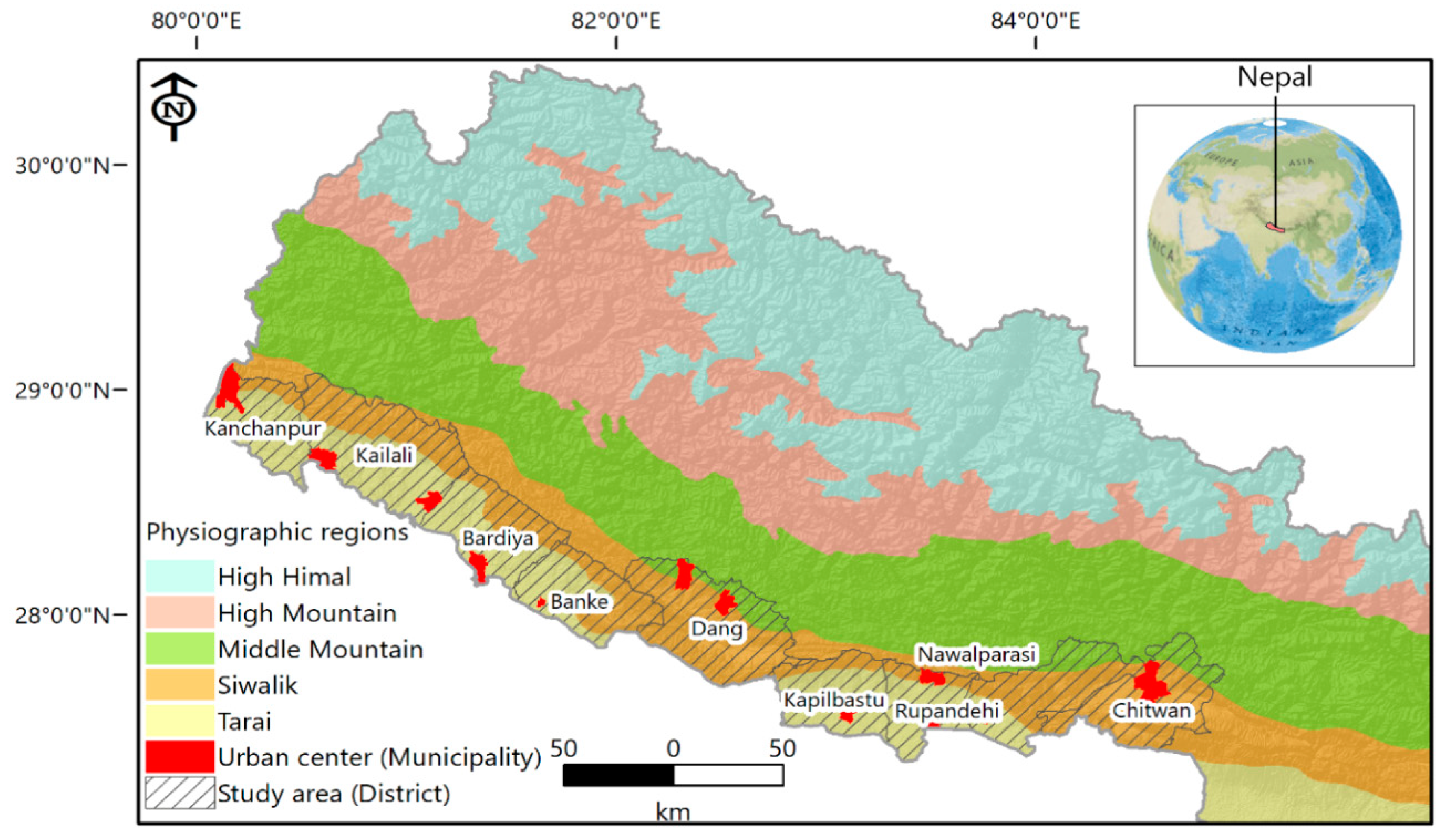
2.1. Study Area
The study area is the western Tarai region of Nepal, covering around 19,200 km2 (Figure 1). The area comprises nine districts (Chitwan, Nawalparasi, Rupandehi, Kapilbastu, Dang, Banke, Bardiya, Kaliali, and Kanchanpur) out of 77 districts nationally. Tarai is relatively flat land and is situated in the low-lying southern region of Nepal, adjoining India. Agriculture and forests are the major land covers of this region, which is the center of national agricultural production. The study area experienced rapid population growth, historically and recently, from 3.2 million residents in 1991 (17% of the national population) to 5.3 million (20%) in 2011 [75]. The study region has a subtropical monsoon climate with temperatures of 32 °C–35 °C during the summer and 8 °C–15 °C during the winter.
2.2. Data
In this study, we observed historical land-cover data derived from surface reflectance (SR) Landsat imagery sourced from various sensors (Landsat 5, Thematic Mapper (TM); Landsat 7, Enhanced Thematic Mapper Plus (ETM+); and Landsat 8, Operational Land Image (OLI)).Land use/cover was classified for the years 1989, 1996, 2001, 2006, 2011, and 2016 [25] and inform our model of historical and future LULC change. Our historical observation period of 1989–2016 are coincident with major LULC trends, particularly migration-led urbanization, the adoption of multiparty democracy in 1990, internal political upheaval of 1996–2006 [23], and the promulgation of a new constitution in 2015 followed by administrative classification.
Landsat provides time-series global imagery since 1972 [76] to cost-effectively describe land-cover change. LULC data were developed using a total 24 surface reflectance (SR) Landsat scenes entailing geometric and atmospheric corrections (for details http://landsat.usgs.gov/CDR_LSR.php). SR data included quality assessment (QA) bands where TM and ETM data were employed [77] and the Landsat 8 OLI-SR data were generated using SR Code (LaSRC) [78]. Before classification all scenes were stacked and subset by district then classified into six different classes: urban/built-up, cultivated land, vegetation cover, barren land, sand cover, and water body. Among various computer-based parametric classification algorithms available, such as parallelepiped, minimum distance (MD) function, maximum likelihood (ML), fuzzy classification (FC) [79], and layer classification (LC) [80], we employed an ML algorithm [25] due to its general familiarity and reliability [81,82].
To assess classification accuracy, we randomly sampled reference points by land-use/cover class. At least 35 sample points were selected for per LULC class per district. The overall accuracy of the annual classifications ranged between 81% and 87% [25], which is generally acceptable upper-level accuracy for such a land-cover classification. The details of the classification accuracies are provided in the Supplementary Materials (Table S1).
Additionally, district-level population data were gathered for the years 1991, 2001, and 2011 from the official census [75]. The data on road networks used to train our model of LULC change were collected from the Nepal Road Network (https://data.humandata.org/dataset/nepal-road-network) and further land cover change data were evaluated using a 1:25,000 topographical map of the Nepalese Survey Department [83] and high-resolution imagery in Google Earth.
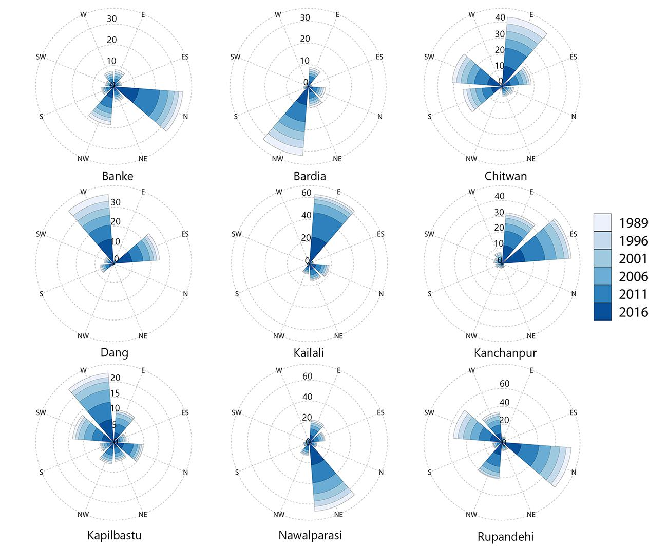
2.3. Urban Expansion Orientation
For each district, the cardinal geographic orientation of urban expansion was observed relative to the primary urban settlement of the district. Here, the “center-point” or origin of urban-expansion orientation is, therefore, the location of this primary urban settlement within a given district, without presupposing that this primary urban settlement is necessarily the commercial or administrative capital of a district [84]. This approach is supported by our field experience and the fact that classified Landsat images of 1989 showed that urban expansion occurred mainly around district headquarters (administrative center) and city centers (commercial centers), which tend to be the primary urban settlements. For the analysis of urban-expansion orientation at the district level, azimuths were drawn at 45° angles from the origin (location of this primary urban settlement) so that a given district was divided into eight quadrants: north to northeast (N–NE), northeast to east (NE–E), east to southeast (E–SE), southeast to south (SE–S), south to southwest (S–SW), southwest to west (SW–W), west to northwest (W–NW), and northwest to north (NW–N).
2.4. Projecting Future Land-Cover Change
Projections of LULC change to 2026 and 2036 were realized using the Land Change Modeler (LCM) within the TerrSet IDRISI software (Clarke Labs 2019, https://clarklabs.org). LCM is an integrated software capable of the LULC change simulation, projection, and validation [85]. The LCM offers three parametric or non-parametric algorithms [48] to evaluate spatial relationships between observed LULC change and predictor variables to effect LULC projection: the multi-layer perceptron (MLP) algorithm artificial neural network, logistic regression, and a similarity-weighted instance-based modeling learning tool [86]. In the present study, we employed the MLP algorithm combined with a Markov chain (MLP–MC) [49] because of its demonstrated accuracy when modeling complex LULC transitions [49,50,55] and relative lack of user-specified coefficients or input maps (as with SLEUTH [54] or CA [53].
The MLP–MC model has a unique advantage when prior knowledge is unavailable, and it can also manage a large number of datasets [51,52]. Its superiority is compared with other models like cellular automata (CA), which need potential transition maps as basic and prior knowledge to handle change procedures [53] or the SLEUTH model, which needs coefficient values to be present [54]. The MLP–MC model was utilized to predict LULC changes in Samsun, Turkey [50], Patna District, India, [49], and Bogor City, Indonesia [55]. All the studies’ results showed that the MLP–MC model was capable of producing the best results in the respective study areas. Therefore, this approach could be a good simulator for identifying the patterns of LULC change in Nepal.
The LULC projection model for western Tarai was developed in three stages corresponding to three temporal periods: calibration (1996–2006), simulation and validation (2006–2016), and projection (2016–2026/2036). Since the MLP–MC model simulates LULC change more accurately for the calibration period than other, later periods (as with any model) [59], LULC in 2016 was projected with the opposite trend of LULC change during 1996–2006. Accordingly, calibration intervals of 10 years (2006–2016) and 20 years (1996–2016) were chosen for the projections of LULC to 2026 and 2036, respectively.
In the first step, the model was calibrated for pixels that transitioned from each land-cover class to other classes between 1996 and 2006. The “transition potentials” for each land-cover transitions (modeled) were defined using a Markov chain, while a sub-model describing transition potentials to urban cover was defined using the multi-layer perceptron (MLP) neural network. Based on other studies on land-change modeling and urban expansion [41,58,87], as well as available data, we used six bio-physical drivers to calibrate our model of the location of LULC during 1996–2006: (i) distance to built-up areas, (ii) distance to cultivated land, (iii) distance to natural vegetation (forests), (iv) distance to roads, (v) distance to water bodies, (vi) elevation and slope. All “distance-based variables” were created based on the Euclidean distance method. Also, natural log and evidence likelihood transformation methods were performed to transform distance-based and categorical factors, respectively. Built-up areas, cultivated lands, and natural vegetation were according to our Landsat classification. Elevation and slope were derived from the digital elevation model (DEM) of the Shuttle Rader Topography Mission (SRTM) 30-m dataset (https://lta.cr.usgs.gov).
The driver data used for model calibration were selected from a larger pool of potential drivers given their relatively strong associations with LULC in the Tarai region (Table 1). Relationships between these drivers and all LULC transitions during the calibration period were examined using Cramer’s coefficient (Table 1). Cramer’s coefficient measures the strength of association between a continuously scaled driver and the probability of a given LULC transition, accounting for both the relationship between each factor and a given LULC class and the relationship between each factor and the total set of LULC classes [88]. This coefficient ranges between 0 and 1, where 1 indicates a maximal association between LULC and the driver, 0 indicates the converse, and > 0.1 indicates an appreciable influence of a driver on LULC processes [89]. Only drivers with strong associations (> 0.1) were retained for the calibration of LULC change, subsequent LULC simulation for validation, and future LULC projections.
In the second step, to validate the model once calibrated, we simulated LULC change between 2006 and 2016, based on trends observed during the calibration period, and then compared the simulated 2016, land-cover map against the 2016 Landsat land-cover classification. The LULC simulation reflects spatial relationships modeled amongst LULC and the “drivers” during the calibration period, but actual observed rates of land-cover change were specified for the simulation over the validation period. Accordingly, measures of error for simulated LULC change pertain exclusively to the location of LULC change, not its quantity. Driver data derived from the Landsat classifications were updated from year one to year two before running the simulation.
Several measures of agreement between the simulated and actual land-cover maps of 2016 were employed, such as kappa variations (Kno, Kstandard, and Klocation) and the figure of merit (FOM). The “Kstandard” index is a measure of the simulated map’s ability to attain perfect classification. The “Klocation” coefficient describes the locational accuracy of pixels in the simulation. The “Kno” index is a modified version of Kstandard and expresses the proportion of correctly classified pixels relative to the expected proportion correctly classified without regard to quantity or location error [90]. The FOM describes the skill of a model to simulate LULC change correctly. It is expressed as the ratio of the area of correctly simulated change against the total area of correctly and incorrectly simulated LULC change or persistence [91]. The FOM is composed of four components, i.e., false alarms (LULC persistence simulated as change), hits (change simulated correctly), misses (change simulated as persistence), and wrong hits (change simulated as change to wrong land-cover class) given by Pontius et al. (2011). Incidentally, the estimation of these components also allow for the disaggregation of total simulation error by LULC quantity and LULC allocation/distribution [92]. The FOM ranges from 0% to 100%, with lower and higher values signifying little agreement and appreciable agreement between actual and simulated change, respectively. Details on the FOM are given by Pontius et al. (2011).
Finally, following model calibration and validation, LULC change was projected forward from 2016 to 2026 and then to 2036 using the Markov chain. The land-cover transition probabilities were again according to the calibration period, while projected rates of LULC were extrapolated from year one and two. Landsat-derived driver data were again updated to 2016 before running the projection.
3. Results
3.1. Historical Land-Cover Change Transitions (1986–2016)
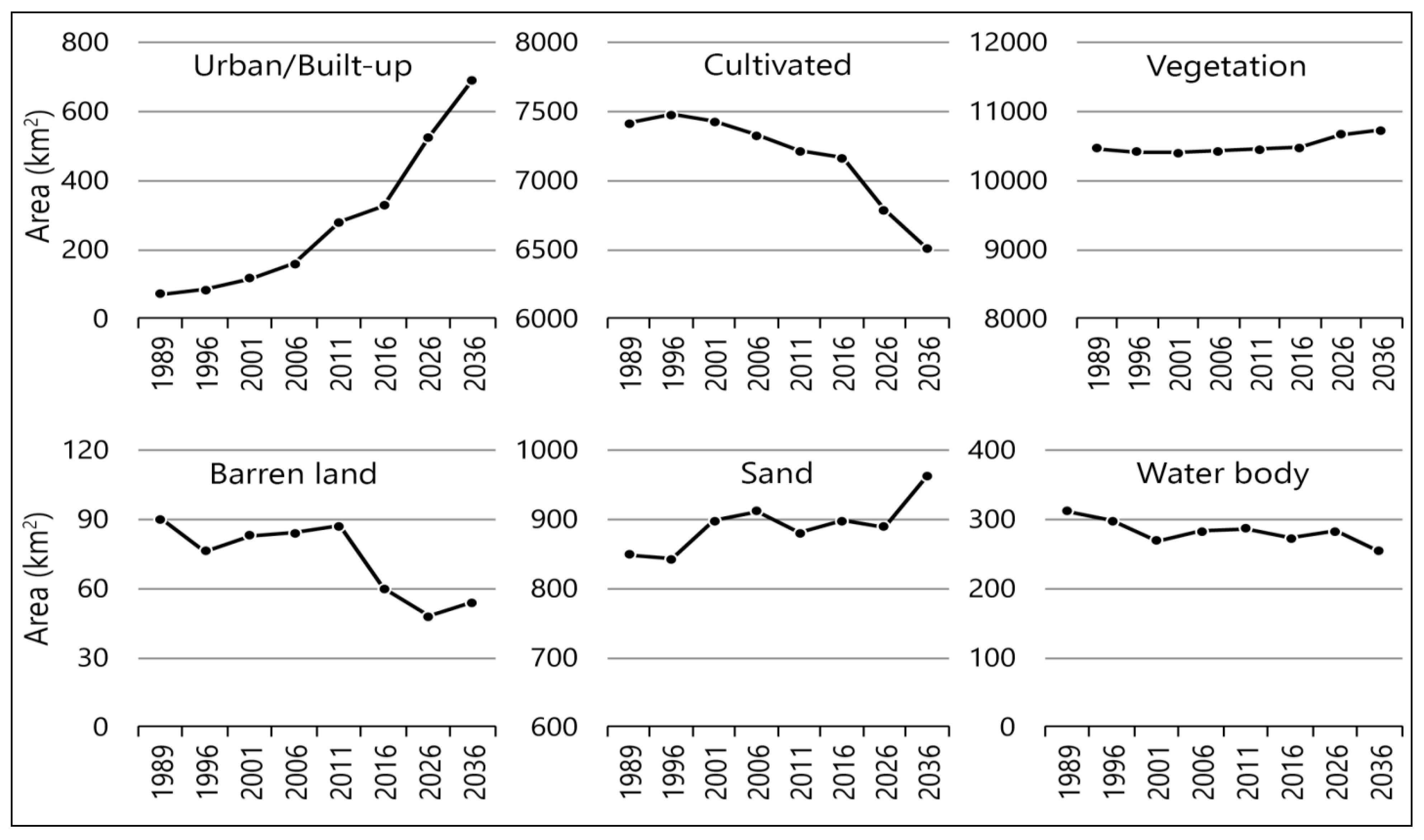
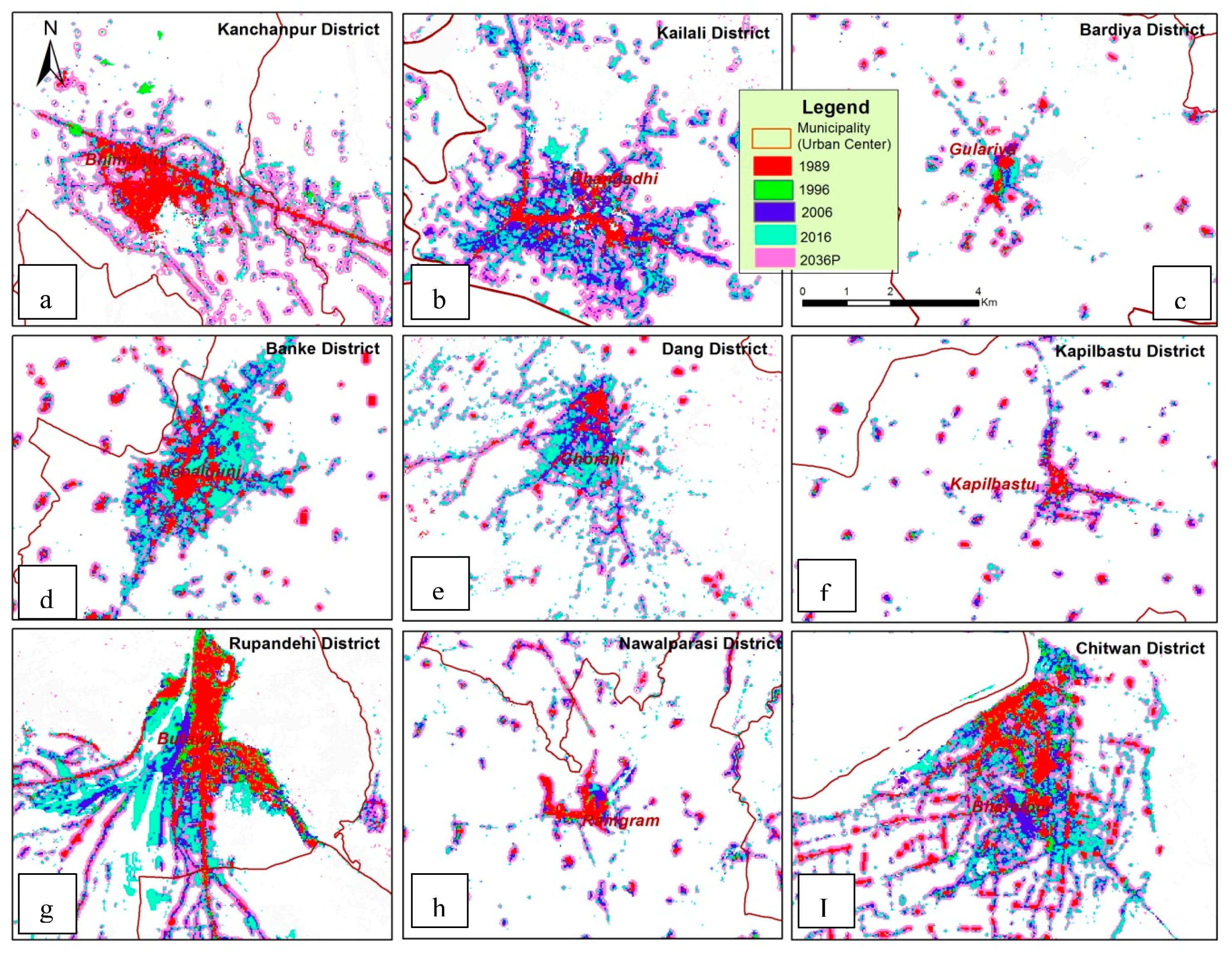
Major trends amongst land-use classes within the study areas between 1989 and 2036 are presented in Table 2 and Figure 2. Urban areas experienced a notable increase historically in terms of both the number of small urban settlements and their total extent. The total urban area expanded by 255.90 km2 between 1989 (71.36 km2) and 2016 (327.26 km2) (Figure 2). The greatest rate of increase in urban expansion over this period (119.45 km2) occurred during 2006–2011, while some (12 km2) occurred during 1989–1996. For all historical periods between 1989 and 2016, urban expansion was characterized by the multiplication and consolidation of smaller “satellite” settlements at the peripheries of major urban centers and along with major road networks (Figure 3), particularly along the East–West highway and North–South highway.
Urban expansion drove a corresponding decrease in cultivated lands. Historically, cultivated lands exhibited a steady decline of 249.47 km2 between 1989 (7411.56 km2) and 2016 (7162.09 km2)—an area of loss almost equal to the coincident increase in urban extent over the same period. This loss of cultivated land tracked contemporary increases in urban cover (Figure 2) as existing urban areas were in-filled and newer settlements expanded outwards over surrounding fertile croplands. The greatest rate of decrease in cultivated lands similarly occurred during 2006–2011 (decrease of 115.22 km2) and 2001–2006 (decrease of 97.45 km2). The Landsat time series also exhibited a non-linear decline for the vegetation cover, sandy areas, and water body classes, but observed no significant contribution of urban expansion to these declines. Figure 3 shows the peripheral expansion of urban/built-up areas from the major city centers of each district of the study area during 1989–2036.
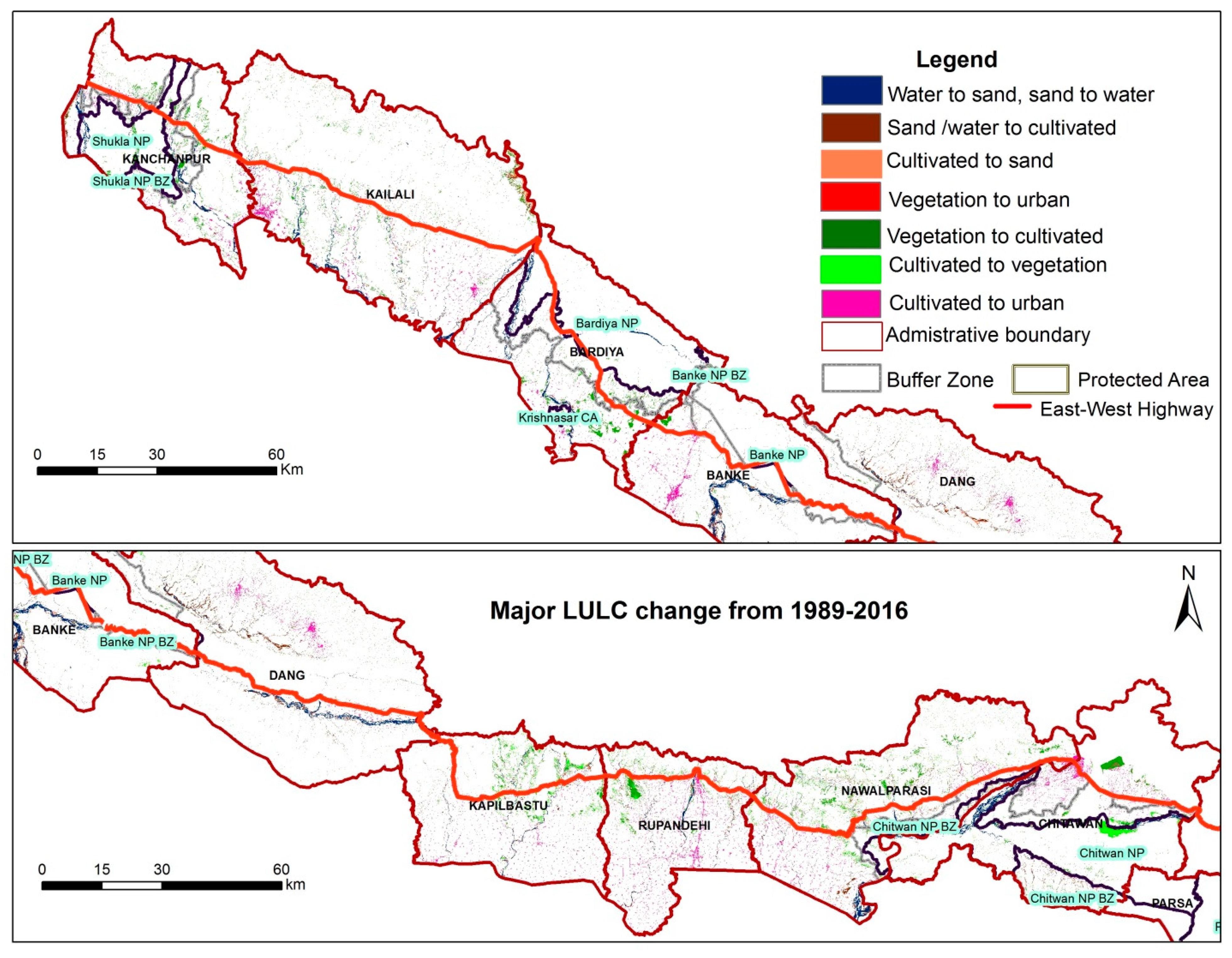
On a broader scale, the transition from cultivated lands to urban cover between 1989 and 1996 was relatively widespread due to the dispersed and patchy pattern of urban expansion (Figure 3 and Figure 4). Extensive areas of agricultural lands were converted to urban areas in the districts of Kailali, Banke, Dang, Rupandehi, and Chitwan (Figure 3b,d,e,g,i). Not only in the urbanizing south, but also in the fertile upland river valleys, transitions from agricultural lands to urban lands predominated and were complemented by lesser extents of transitions from forested lands to urban cover. However, in the northern uplands, cultivated land areas also transitioned to natural vegetation, largely as fallows, planted woodlands, and natural forest regeneration. Notably, such reforestation of historically cultivated areas occurred at the fringes of protected areas, including Chitwan National Park, Parsa Wildlife Reserve, Shuklaphanta National Park, Banke National Park, and Bardiya National Park. It is unknown whether the recovery of forests reflected trends in the management of protected areas or a larger trend in the extensification and/or abandonment of peripheral agricultural production due to rural–urban migration and agricultural intensification.
3.2. Urban-Expansion Orientation
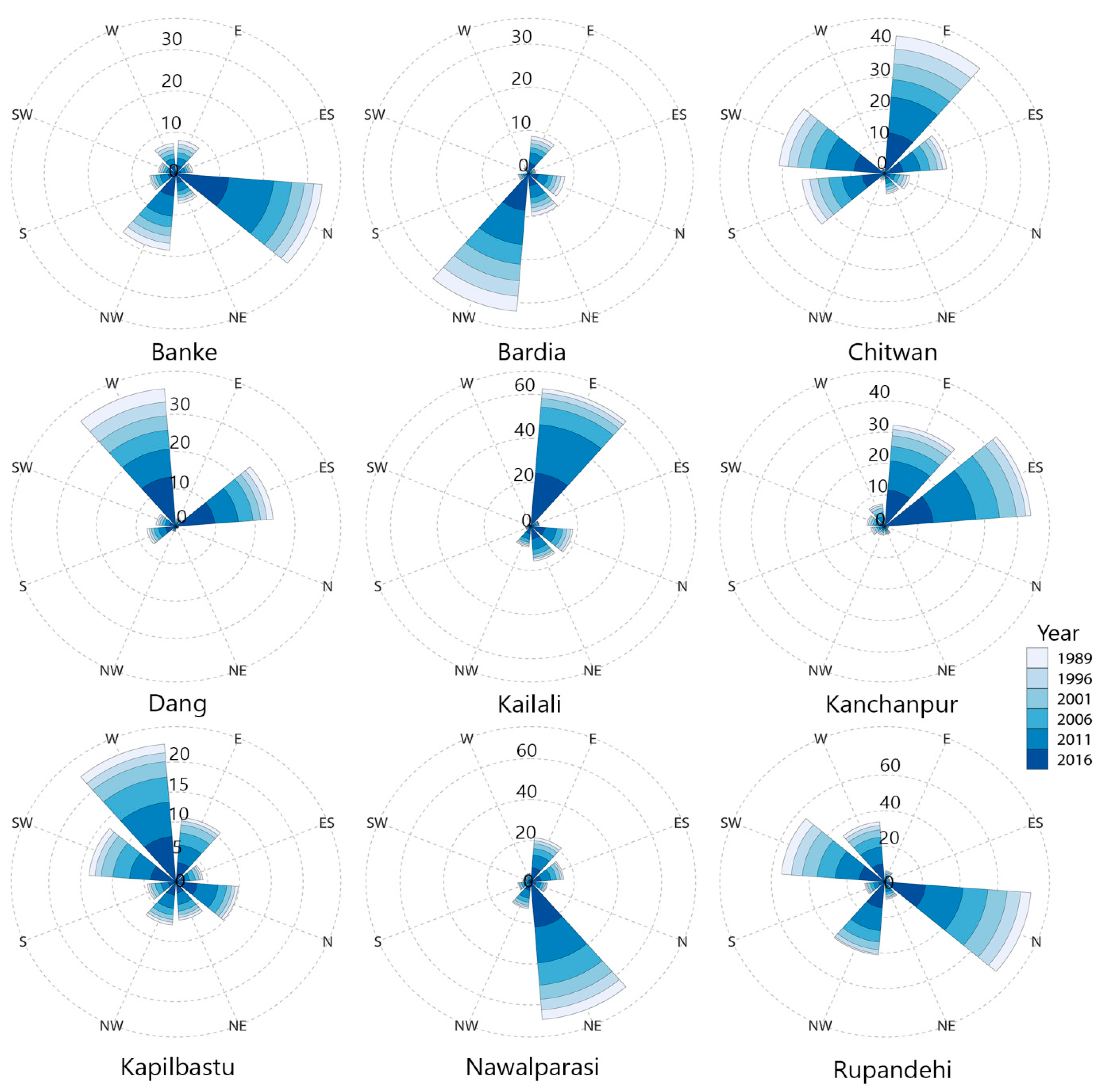
The primary urban centers of all districts except for Dang, Kanchanpur, Chitwan, and Bara were located in the southern part of their respective districts. Hence, urban expansion in the earlier decades generally expanded to north, northeast, and northwest of these primary urban centers. Conversely, in Kanchanpur district, urban expansion was mainly toward the southeast and eastern peripheries. The highest urban expansion of Dang was toward the western and southeastern directions from the district headquarter, while the eastern parts followed by southwest and southeast directions of Chitwan district were highly urbanized. An urban expansion orientation of individual districts is presented in Figure 5.
Urbanization took place mainly at the periphery of the East–West highway, Postal highway, and the connecting road networks to the mid-hills. Additionally, the areas which were easily accessible from the mid-hill districts were rapidly expanded. For example, some of the major urban centers in the East–West highway (Figure 4) were Ratnanagar, Bharatpur, Gaidakot, Kawasoti, Bardaghat, Sunaul, Devdaha, Lamahi, Attariya, Kohalpur, and Mahendranagar. Additionally, Taulihawa, Butwal, Krishnanagar, Nepalgunj, Dhangadhi, Gaur, Ghorahi, and Tulsipur were the other centers. In those areas, settlements were scattered, and agricultural lands were plotted for residential purposes and, thus, were fragmented.
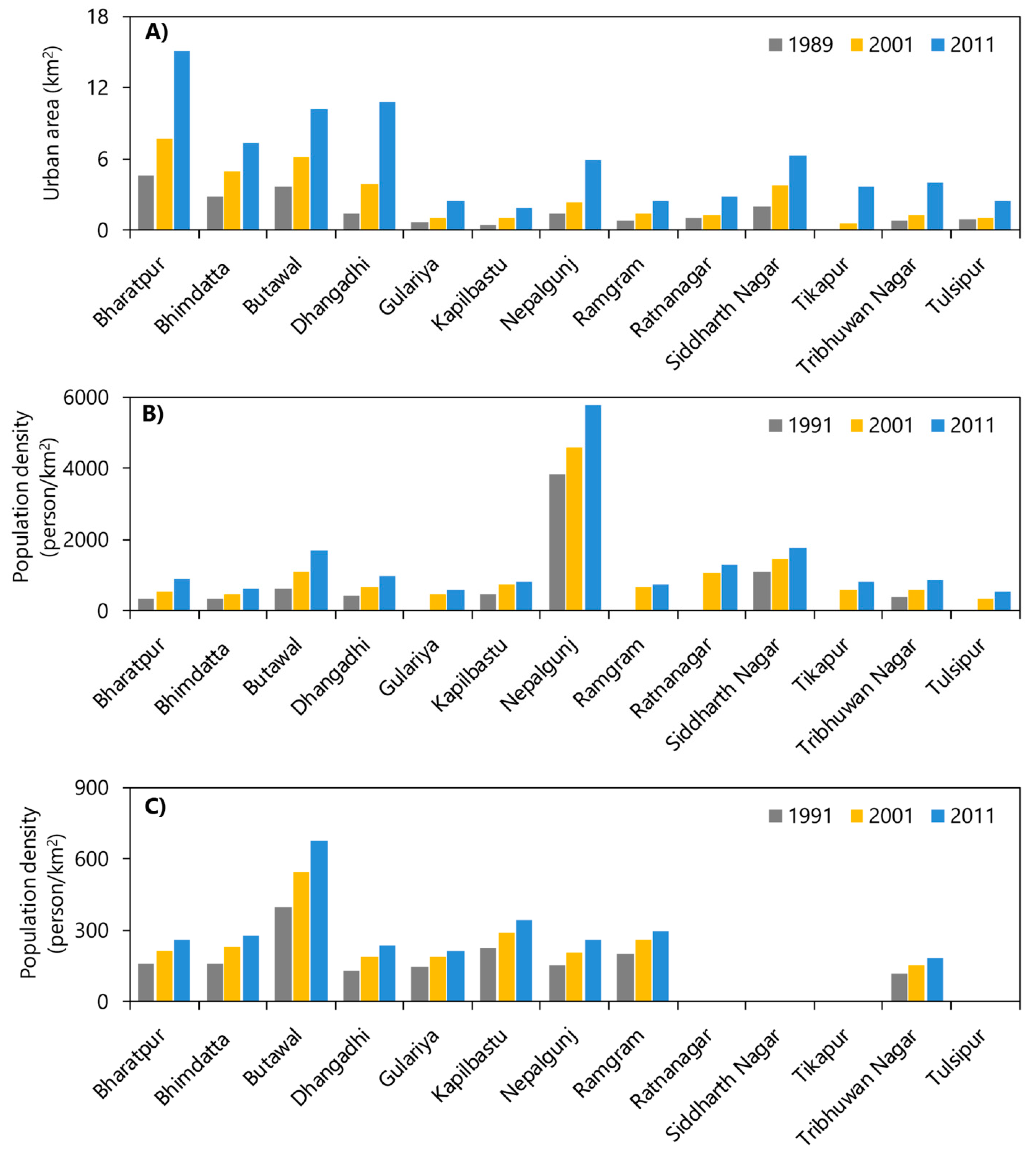
Spatially, the existing urban agglomerations were in-filled or expanded along the peripheries of major highways and cities. Population density was increasingly high and unequally distributed within the districts as expanding urban extents hosted an increasing majority of district populations (Figure 6). For instance, the population density of Nepalgunj Municipality (NM) of Banke was 3824 persons/km2 in 1991 and increased to 4601 and 5798 persons/km2 in 2001 and 2011, respectively. Similar trends were seen in Bharatpur, Butwal, Siddarthanagar, Dhangadi, and Tikapur municipalities of Chitwan, Rupandehi, Banke, and Kailaili districts (Figure 6).
3.3. Land-Cover Change Simulation and Projections to 2026 and 2036
Based on historical LULC trends between 1989 and 2016, LULC of 2026 and 2036 was projected using artificial neural network land-cover transition probabilities adjusted using an MLP–MC spatial model. The resultant projections indicated a continued decline in cultivated lands due to urban expansion, as well as lesser fluctuations amongst the other LULC classes. Urban/built-up area is projected to expand by over 110% of its 2016 extent by 2036, entailing an average annual growth rate of 3.8% if compounded annually and of 5.5% if not, with both rates being greater than national annual demographic growth rates of 1–2.7% since 1970. Such urban growth would entail an additional increase of urban cover of 199 km2 by 2026 (total to 526.05 km2) and an additional 364.15 km2 by 2036 (total 691.20 km2), up from 327.05 km2 in 2016 (Table 3 and Figure 7).
Correspondingly, cultivated lands in the future are expected to decline due to permanent losses from urbanization, notwithstanding minor dynamic exchanges between agriculture and natural vegetation. Of the 199 km2 of additional urban cover projected from 2016 to 2026, 99% (187.39 km2) is expected to derive from cultivated land and the remainder (11.97 km2) is expected to derive from vegetation cover. Over the same period, an additional and comparable 165.61 km2 of cultivated lands would be brought into production by converting natural vegetation cover. In this way, trends in the urban expansion are observed to drive losses not only of agriculture directly but also of natural vegetation indirectly, as agricultural losses due to urban conversion may spur agricultural expansion elsewhere at the cost of natural vegetation. Despite this projected addition of new cultivated lands, the total net agricultural area would still decline by 377.19 km2 (Table 4) over 2016–2026 due to urbanization. While nominal losses of cultivated lands due to urbanization over 2016–2026 are lesser than losses of agricultural land due to recovered natural vegetation over the same period (310 km2), some of these later projected losses are likely temporary due to agricultural fallowing.
Trends of urban expansion and agriculture land loss during 2026–2036 were largely similar to those for 2016–2026, if slightly more moderate with respect to rates of urban expansion. Urban/built-up areas would expand further by 165.16 km2, with a more moderate average annual growth rate of 2.7% (annually compounded) or 3.1% (not compounded). Of this additional urban increase, 95% would be sourced from cultivated land. Despite the establishment of 162 km2 new cultivated lands due to natural vegetation conversion, total cultivated area would still decline by 277 km2 due to transitions to urban cover (156 km2), as well as to vegetation cover (234 km2) and sand (attributable to flooding and erosion of cultivated riverine valleys) (83.53 km2) (Table 5).
The projection models signal a declining yet still high rate of urban expansion and corresponding losses of cultivated lands. The historical Landsat observations describe average annual rates of urban expansion of 9–10% during 1996–2006 and 2006–2016 (rates here are not compounded). In contrast, lesser rates of 6.08% and 3.13% were projected for 2016–2026 and 2026–2036, respectively. Perhaps as a result of declining future urbanization rates, the proportion of newly established urban areas derived from the cultivated land area during 2026–2036 is slightly lower (94.91%) than during 2016–2026 (99%).
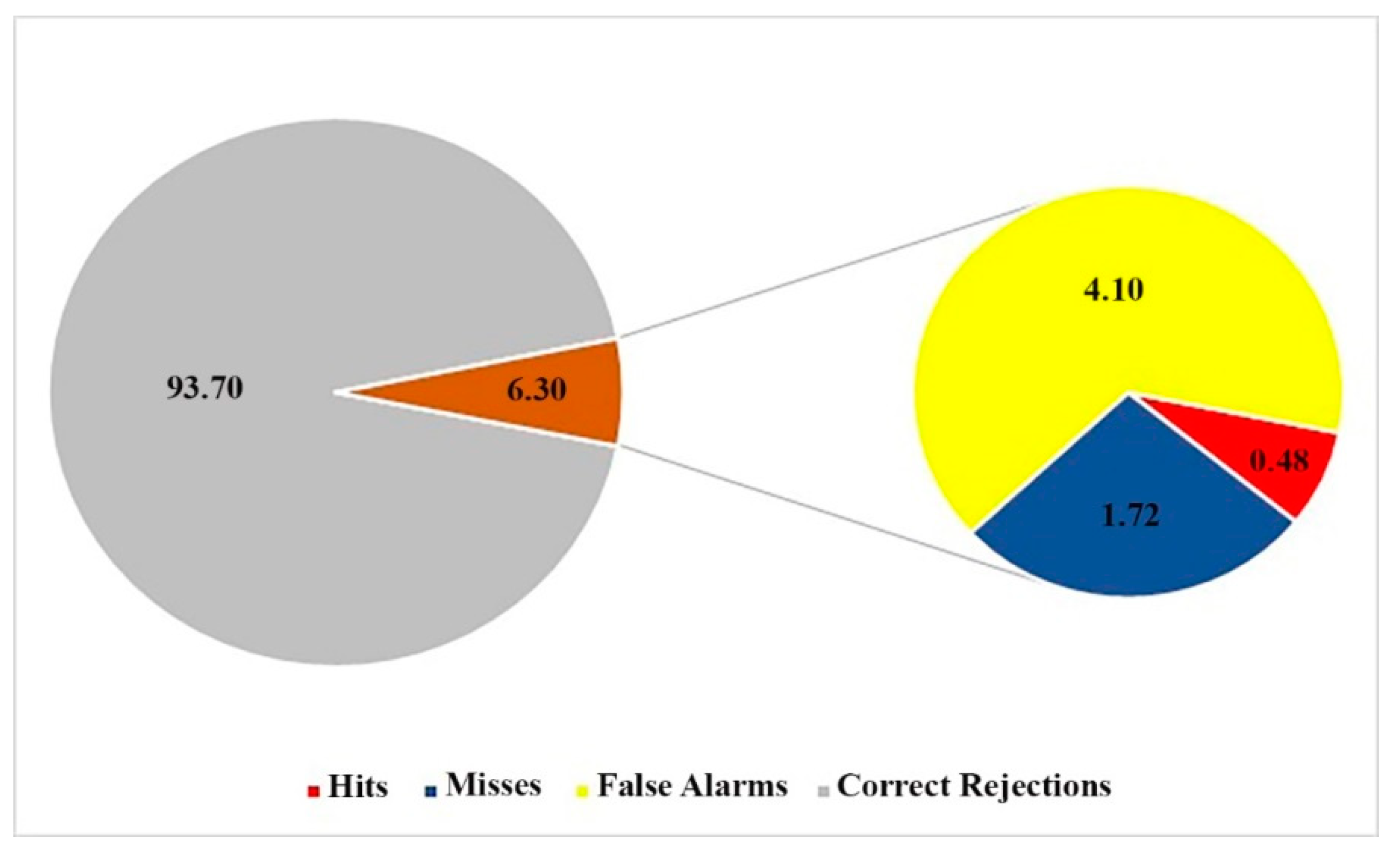
The results of our accuracy assessment showed that the standard accuracy of the model was more than 80%, which means that the model was effective in prediction [59,93,94]. The evaluation implied that the value of Kno was 0.88, which verified the accuracy of the model. The overall ability of the model to simulate the LULC map of 2016 was highly assessed in general (Kstandard = 0.83), and the Klocation value of 0.90 detected that the model prepared a logical representation of the location. The analysis of modeling shows that the FOM was 0.08%. According to Figure 8, hits accounted for 0.48% of the spatial extent. The components of misses and false alarms were 1.72% and 4.10%, respectively. Furthermore, the values for the reference change simulated as a change to the wrong category (wrong hits) were zero. Accordingly, the quantity error was 2.38%, while the allocation error was 3.43% of the spatial extent.
4. Discussion
The spatiotemporal changes in land use in western Tarai of Nepal during 1989–2016 highlight the rapid growth of urban areas and corresponding losses of cultivated areas. Projections of urban expansion to 2026 and 2036 indicate the continuation of such trends. Notwithstanding the projected decline in urban-expansion rates, rapid urban growth and agricultural loss will continue largely unabated.
Our LULC simulation indicates two major land-change transformations characterizing western Nepal, namely, rapid urban expansion and the loss of agricultural land. The spatial patterns of scattered, small-scale “satellite” urban expansion and linear “in-fill” urbanization along the side of highways suggests that urban growth is not pre-emptively zoned and managed at the local level. The commonly observed weakness of local government in formulating and enforcing land-use zones and plans [17,56] doubtlessly facilitated the haphazard pattern of urban expansion regionally and is anticipated to persist in the future.
According to the historical LULC trend analysis, the extent of urban expansion relative to other land-cover changes varied markedly by the period. Such variation is associated with several underlying socioeconomic factors, political events, and changing access to public services [25,66]. Our analysis shows that urban expansion accelerated after 2001, which may reflect increased rural–urban migration caused by the domestic political conflict that occurred between 1996 and 2006 [23]. Meanwhile, the greatest expansion in the urban areas occurred during 2006–2011, which may reflect the legacy of the prior surge of urban migrants to 2006 and related resumption of urban economic development. Nonetheless, the migration pattern reflects both push factors (e.g., rural poverty) and pull factors (e.g., better public services and economic opportunities) [25,69].
It is notable that cultivated areas in Nepal are often located near urban areas, and there is, therefore, inherent competition for these lands amongst farmers and urban developers. As in Nepal, such competition and ultimate expansion of urban cover over arable lands is observed widely in many developing-world contexts. Indeed, transition probabilities from cultivated lands to built-up lands reported by similar spatial studies elsewhere are similarly extremely high [5,46,47,87,89,95,96].
The implications of projected net agricultural contraction over 2016–2026 are uncertain and potentially serious, depending on underlying land-use dynamics. The apparent re-vegetation of peripheral upland agricultural areas is commensurate with the abandonment of underproductive, marginal agricultural areas and related rural-to-urban migration [97,98]. If agricultural intensification occurs simultaneously with ongoing agricultural contraction, regional food security might remain stable despite the contractions. This possibility is, however, undermined by the slightly lesser but still substantial losses of relatively fertile, per-urban agricultural lands due to urban expansion. Clearly, food security also depends on the degree to which the apparent re-vegetation of agricultural uplands is due to permanent land abandonment or rather its transition to ephemeral fallows or productive tree crops [99]. The permanence of agricultural losses to urban covers, as well as their concentration in fertile per-urban zones and floodplains, highlights serious implications for national agricultural productivity [100]. Our study area is characterized by fertile land and is considered highly important for national grain and pulse production [101].
Generally, urbanization follows an “S-shaped” maturation trend described by initial slow urban development, then rapid expansion and, finally, slow consolidation [102,103]. Our Nepalese case study does not adhere to this general trend well, indicating either that Nepalese urbanization is still in its middling phases and/or that the maturation trend is not inevitable. Therefore, the prediction of future urban growth is prudent to help steer developments toward sound sustainable consolidation as soon as possible [104]. As this study underscores, such outcomes are relevant for per-urban areas but may also have broader implications for land-use change elsewhere. As the scale of urbanization grows, urbanization policy in developing countries is expected to influence land-use changes more widely [103], e.g., as in regard to regional water resource availability, green belts, and erosion control.
Although this study used a wide variety of data and robust methodology, it has several limitations that should be recognized as opportunities for further research. This study could not consider various probable drivers of urban expansion, such as local population growth, government policy, agricultural market demand (land rents), and so on due to a lack of spatial data and reliable means of associating such drivers with spatially explicit land-cover change. Complex processes driven by dynamic non-linear or spatial interactions shape land change and are difficult to capture using available data and algorithms [105]. Such missing factors may significantly affect the LULC trajectory of future urban expansion and agricultural loss, such that our projections are best understood exclusively as extensions of the trends and data observed. Future land-change scenarios in which urban expansion is limited to lands zoned for this purpose should particularly be considered as a means of gauging the utility of current land-use plans for future food security. We also acknowledge large uncertainties in our estimations. Our spatial model is based on historical land-change transitions; thus, its projections will diverge from reality should future trends in LULC change depart from the past. Similarly, our results may differ from those based on historical observations employing an alternative typology of land-cover classes. Indeed, the land-use/cover maps used for LULC modeling were derived from the 30-m resolution Landsat imagery, the resolution of which limited both the range and the accuracy of observable land-cover classes. In the future, high-resolution satellite data (e.g., SPOT satellite or WorldView) could be used to derive more diverse and thematically precise observations of particular agricultural and urban covers relevant to agricultural loss and food security, e.g., subsistence vs. mechanized cultivation, or sprawling vs. high-density urban cover. The use of high-resolution imagery may even prove especially useful in estimating the productivity of agricultural lands that are converted, abandoned, and newly established, thus further refining estimates of changing food security. Nonetheless, our simulation helps to understand, forecast, and anticipate the future in the likely event that the future reflects the past.
5. Conclusions
This study investigated the major LULC transformations in the western Tarai region of Nepal during 1989–2016 and examined the future trends to 2026 and 2036 using an artificial neural network–Markov chain spatial model. The major transformations observed include a continuous expansion of urban/built-up area, the corresponding decline of cultivated land, and non-linear changes in forest cover. Rapid increases in urban cover and losses to agricultural areas are expected to continue at only slightly reduced rates. The average annual urban growth rate is projected to decline from 13.35% during 1989–2016 to 5.56% during 2016–2036.
The continued rapid and largely unplanned expansion of urban cover and the corresponding decline of cultivated land may have serious consequences for food security and environmental sustainability. The nature of such consequences depends on the nature of peripheral agricultural land use, land abandonment and revegetation, and any economic “feedback” to the national agricultural market. A long-term sustainable urban-expansion plan is essential to promote orderly urbanization and should be linked to similarly urgent plans for agricultural resilience. The research presented here may serve such purposes. Urban growth models saw rapid development and extensive adoption. Furthermore, the emergence of freely available spatial data and the reduction in computational costs offer opportunities to model change at finer resolutions and/or greater extents. We recommend that future studies continue to explore these models and data to develop simulations addressing future LULC uncertainties.
Supplementary Materials
The following are available online at https://0-www-mdpi-com.brum.beds.ac.uk/2072-4292/12/4/628/s1, Table S1: Landsat Land-use/cover classification accuracies by district and year, Table S2: The absolute and relative areas of land-use/cover classes in western Tarai by year (km2), Table S3. Land-use/cover class transition probability matrix calculated using pairs of Landsat classifications for 1996–2006, 2006–2016, and 1996–2016.
Author Contributions
Conceptualization, B.R.; methodology, B.R., H.K.; software and writing—original draft preparation, B.R., S.S., H.K., R.S., S.R. and U.B.S.; writing—review and editing, B.R., S.S., H.K., R.S., S.R. and U.B.S.; visualization, B.R., U.B.S. All authors have read and agreed to the published version of the manuscript.
Funding
This research received no external funding.
Conflicts of Interest
The authors declare no conflict of interest.
References
- Foley, J.A.; DeFries, R.; Asner, G.P.; Barford, C.; Bonan, G.; Carpenter, S.R.; Chapin, F.S.; Coe, M.T.; Daily, G.C.; Gibbs, H.K.; et al. Global consequences of land use. Science 2005, 309, 570–574. [Google Scholar] [CrossRef] [Green Version]
- Turner, B.L.; Lambin, E.F.; Reenberg, A. The emergence of land change science for global environmental change and sustainability. Proc. Natl. Acad. Sci. USA 2007, 104, 20666–20671. [Google Scholar] [CrossRef] [Green Version]
- Gibbs, H.K.; Ruesch, A.S.; Achard, F.; Clayton, M.K.; Holmgren, P.; Ramankutty, N.; Foley, J.A. Tropical forests were the primary sources of new agricultural land in the 1980s and 1990s. Proc. Natl. Acad. Sci. USA 2010, 107, 16732–16737. [Google Scholar] [CrossRef] [Green Version]
- He, C.; Liu, Z.; Gou, S.; Zhang, Q.; Zhang, J.; Xu, L. Detecting global urban expansion over the last three decades using a fully convolutional network. Environ. Res. Lett. 2018, 14, 034008. [Google Scholar] [CrossRef]
- Angel, S.; Parent, J.; Civco, D.L.; Blei, A.; Potere, D. The dimensions of global urban expansion: Estimates and projections for all countries, 2000–2050. Prog. Plan. 2011, 75, 53–107. [Google Scholar] [CrossRef]
- Seto, K.C.; Güneralp, B.; Hutyra, L.R. Global forecasts of urban expansion to 2030 and direct impacts on biodiversity and carbon pools. Proc. Natl. Acad. Sci. USA 2012, 109, 16083–16088. [Google Scholar] [CrossRef] [Green Version]
- UNDESA. World Urbanization Prospects: The 2018 Revision; United Nation Development of Economic and Social Affairs, United Nation: Bangkok, Thailand, 2018. [Google Scholar]
- IPBES. Ipbes global assessment on biodiversity and ecosystem services. In Intergovernmental Science-Policy Platform on Biodiversity and Ecosystem Services (IPBES); IPBES: Paris, France, 2019. [Google Scholar]
- Van Ginkel, H. Urban future. Nature 2008, 456, 32. [Google Scholar] [CrossRef]
- Dewan, A.M.; Corner, R.J. Spatiotemporal analysis of urban growth, sprawl and structure. In Dhaka Megacity, Geospatial Perspectives on Urbanization, Environment and Health; Springer: New York, NY, USA, 2013. [Google Scholar]
- d’Amour, C.B.; Reitsma, F.; Baiocchi, G.; Barthel, S.; Güneralp, B.; Erb, K.-H.; Haberl, H.; Creutzig, F.; Seto, K.C. Future urban land expansion and implications for global croplands. Proc. Natl. Acad. Sci. USA 2017, 114, 8939–8944. [Google Scholar] [CrossRef] [PubMed] [Green Version]
- Van Vliet, J.; Eitelberg, D.A.; Verburg, P.H. A global analysis of land take in cropland areas and production displacement from urbanization. Glob. Environ. Chang. 2017, 43, 107–115. [Google Scholar] [CrossRef]
- Zhao, S.; Da, L.; Tang, Z.; Fang, H.; Song, K.; Fang, J. Ecological consequences of rapid urban expansion: Shanghai, China. Front. Ecol. Environ. 2006, 4, 341–346. [Google Scholar] [CrossRef]
- Grimm, N.B.; Faeth, S.H.; Golubiewski, N.E.; Redman, C.L.; Wu, J.; Bai, X.; Briggs, J.M. Global change and the ecology of cities. Science 2008, 319, 756–760. [Google Scholar] [CrossRef] [PubMed] [Green Version]
- Linard, C.; Tatem, A.J.; Gilbert, M. Modelling spatial patterns of urban growth in africa. Appl. Geogr. (Sevenoaksengland) 2013, 44, 23–32. [Google Scholar] [CrossRef] [PubMed]
- Henderson, V. Urbanization in developing countries. World Bank Res. Obs. 2002, 17, 89–112. [Google Scholar] [CrossRef]
- Bhattarai, K.; Conway, D. Urban vulnerabilities in the kathmandu valley, Nepal: Visualizations of human/hazard interactions. J. Geogr. Inf. Syst. 2010, 02, 63–84. [Google Scholar] [CrossRef] [Green Version]
- MoFALD. Local Level Reconstruction Report; Ministry of Federal Affairs and Local Development (MoFALD), Nepal Government: Kathmandu, Nepal, 2017.
- Rimal, B.; Keshtkar, H.; Sharma, R.; Stork, N.; Rijal, S.; Kunwar, R. Simulating urban expansion in a rapidly changing landscape in eastern tarai, nepal. Environ. Monit. Assess. 2019, 191, 255. [Google Scholar] [CrossRef] [PubMed]
- MoUD. National urban Development Strategy (NUDS) 2015; Government of Nepal, Ministry of Urban Development: Kathmandu, Nepal, 2015.
- WHO. Nepal Malaria Programme Review World Health Organization (WHO); Regional Office for South-East Asia Ed: New Delhi, India, 2011. [Google Scholar]
- Shrestha, N.R. Landlessness and Migration in Nepal; Westview Press: Oxford, UK, 1990. [Google Scholar]
- Muzzini, E.; Gabriela, A. Urban Growth and Spatial Transition in Nepal; The World Bank: Washington, DC, USA, 2013. [Google Scholar]
- Gartaula, H.; Niehof, A. Migration to and from the terai: Shifting movements and motives. Southasianist 2013, 2, 29–51. [Google Scholar]
- Rimal, B.; Zhang, L.; Stork, N.; Sloan, S.; Rijal, S. Urban expansion occurred at the expense of agricultural lands in the tarai region of Nepal from 1989 to 2016. Sustainability 2018, 10, 1341. [Google Scholar] [CrossRef] [Green Version]
- Uddin, K.; Shrestha, H.L.; Murthy, M.S.; Bajracharya, B.; Shrestha, B.; Gilani, H.; Pradhan, S.; Dangol, B. Development of 2010 national land cover database for the nepal. J. Environ. Manag. 2015, 148, 82–90. [Google Scholar] [CrossRef]
- Dewan, A.M.; Yamaguchi, Y. Using remote sensing and gis to detect and monitor land use and land cover change in dhaka metropolitan of bangladesh during 1960–2005. Environ. Monit. Assess. 2009, 150, 237–249. [Google Scholar] [CrossRef]
- Rimal, B.; Zhang, L.; Keshtkar, H.; Sun, X.; Rijal, S. Quantifying the spatiotemporal pattern of urban expansion and hazard and risk area identification in the kaski district of nepal. Land 2018, 7, 37. [Google Scholar] [CrossRef] [Green Version]
- Rijal, S.; Rimal, B.; Sloan, S. Flood hazard mapping of a rapidly urbanizing city in the foothills (birendranagar, surkhet) of Nepal. Land 2018, 7, 60. [Google Scholar] [CrossRef] [Green Version]
- Rimal, B.; Sharma, R.; Kunwar, R.; Keshtkar, H.; Stork, N.E.; Rijal, S.; Rahman, S.A.; Baral, H. Effects of land use and land cover change on ecosystem services in the koshi river basin, eastern Nepal. Ecosyst. Serv. 2019, 38, 100963. [Google Scholar] [CrossRef]
- Rai, R.; Zhang, Y.; Paudel, B.; Acharya, B.; Basnet, L. Land use and land cover dynamics and assessing the ecosystem service values in the trans-boundary gandaki river basin, central himalayas. Sustainability 2018, 10, 3052. [Google Scholar] [CrossRef] [Green Version]
- Liping, C.; Yujun, S.; Saeed, S. Monitoring and predicting land use and land cover changes using remote sensing and gis techniques—A case study of a hilly area, jiangle, china. PLoS ONE 2018, 13, e0200493. [Google Scholar] [CrossRef]
- Eastman, J.R.; van Fossen, M.E.; Solarzano, L.A. Transition Potential Modeling for Land-Cover Change, 1st ed.; ESRI Press: Redlands, CA, USA, 2005. [Google Scholar]
- Sloan, S.; Zamora Pereira, J.C.; Labbate, G.; Asner, G.P.; Imbach, P. The cost and distribution of forest conservation for national emissions reductions. Glob. Environ. Chang. 2018, 53, 39–51. [Google Scholar] [CrossRef]
- Alqurashi, A.F.; Kumar, L.; Sinha, P. Urban land cover change modelling using time-series satellite images: A case study of urban growth in five cities of saudi arabia. Remote Sens. 2016, 8, 838. [Google Scholar] [CrossRef] [Green Version]
- Tallis, H.; Polasky, S. Mapping and valuing ecosystem services as an approach for conservation and natural-resource management. Ann. N. Y. Acad. Sci. 2009, 1162, 265–283. [Google Scholar] [CrossRef]
- Rodrigues, H.; Soares-Filho, B. A short presentation of dinamica ego. In Geomatic Approaches for Modeling Land Change Scenarios; Camacho Olmedo, M.T., Paegelow, M., Mas, J.-F., Escobar, F., Eds.; Springer International Publishing: Cham, Germany, 2018; pp. 493–498. [Google Scholar]
- Clarke, K.C. Land use change modeling with sleuth: Improving calibration with a genetic algorithm. In Geomatic Approaches for Modeling Land Change Scenarios; Camacho Olmedo, M.T., Paegelow, M., Mas, J.-F., Escobar, F., Eds.; Springer International Publishing: Cham, Germany, 2018; pp. 139–161. [Google Scholar]
- Theobald, D. Landscape patterns of exurban growth in the USA from 1980 to 2020. Ecol. Soc. 2005, 10, 34. [Google Scholar] [CrossRef] [Green Version]
- Verburg, P.H.; Overmars, K.P. Dynamic simulation of land-use change trajectories with the clue-s model. In Modelling Land-Use Change: Progress and Applications; Koomen, E., Stillwell, J., Bakema, A., Scholten, H.J., Eds.; Springer: Dordrecht, The Netherlands, 2007; pp. 321–337. [Google Scholar]
- Sloan, S.; Pelletier, J. How accurately may we project tropical forest-cover change? Glob. Environ. Chang. 2012, 22, 440–453. [Google Scholar] [CrossRef]
- Sleeter, B.M.; Wood, N.J.; Soulard, C.E.; Wilson, T.S. Projecting community changes in hazard exposure to support long-term risk reduction: A case study of tsunami hazards in the U.S. Pacific northwest. Int. J. Disaster Risk Reduct. 2017, 22, 10–22. [Google Scholar] [CrossRef] [Green Version]
- Yang, X.; Chen, R.; Zheng, X.Q. Simulating land use change by integrating ann-ca model and landscape pattern indices. Geomat. Nat. Hazards Risk 2016, 7, 918–932. [Google Scholar] [CrossRef] [Green Version]
- Kuo, H.-F.; Tsou, K.-W. Modeling and simulation of the future impacts of urban land use change on the natural environment by sleuth and cluster analysis. Sustainability 2018, 10, 72. [Google Scholar] [CrossRef] [Green Version]
- Veldkamp, A.; Fresco, L.O. Clue: A conceptual model to study the conversion of land use and its effects. Ecol. Model. 1996, 85, 253–270. [Google Scholar] [CrossRef]
- Jokar Arsanjani, J.; Helbich, M.; Kainz, W.; Darvishi Boloorani, A. Integration of logistic regression, markov chain and cellular automata models to simulate urban expansion. Int. J. Appl. Earth Obs. Geoinf. 2013, 21, 265–275. [Google Scholar] [CrossRef]
- Pahlavani, P.; Askarian Omran, H.; Bigdeli, B. A multiple land use change model based on artificial neural network, markov chain, and multi objective land allocation. Earth Obs. Geomat. Eng. 2017, 1, 82–99. [Google Scholar]
- Sangermano, F.; Toledano, J.; Eastman, R. Land cover change in the bolivian amazon and implications for redd+ and endemic biodiversity. Land 2012, 27, 571–584. [Google Scholar] [CrossRef]
- Mishra, V.N.; Rai, P.K. A remote sensing aided multi-layer perceptron-markov chain analysis for land use and land cover change prediction in patna district (bihar), India. Arab. J. Geosci. 2016, 9, 249. [Google Scholar] [CrossRef]
- Ozturk, D. Urban growth simulation of atakum (samsun, turkey) using cellular automata-markov chain and multi-layer perceptron-markov chain models. Remote Sens. 2015, 7, 5918–5950. [Google Scholar] [CrossRef] [Green Version]
- Riccioli, F.; El Asmar, T.; El Asmar, J.-P.; Fagarazzi, C.; Casini, L. Artificial neural network for multifunctional areas. Environ. Monit. Assess. 2015, 188, 67. [Google Scholar] [CrossRef] [PubMed]
- Iizuka, K.; Johnson, B.A.; Onishi, A.; Magcale-Macandog, D.B.; Endo, I.; Bragais, M. Modeling future urban sprawl and landscape change in the laguna de bay area, philippines. Land 2017, 6, 26. [Google Scholar] [CrossRef]
- Pontius, R.G.; Boersma, W.; Castella, J.-C.; Clarke, K.; de Nijs, T.; Dietzel, C.; Duan, Z.; Fotsing, E.; Goldstein, N.; Kok, K.; et al. Comparing the input, output, and validation maps for several models of land change. Ann. Reg. Sci. 2008, 42, 11–37. [Google Scholar] [CrossRef] [Green Version]
- Chaudhuri, G.; Clarke, K. The sleuth land use change model: A review. Int. J. Environ. Resour. Res. 2013, 1, 88–105. [Google Scholar]
- Nurwanda, A.; Honjo, T. The prediction of city expansion and land surface temperature in bogor city, indonesia. Sustain. Cities Soc. 2020, 52, 101772. [Google Scholar] [CrossRef]
- Thapa, R.B.; Murayama, Y. Scenario based urban growth allocation in kathmandu valley, nepal. Landsc. Urban Plan. 2012, 105, 140–148. [Google Scholar] [CrossRef]
- Haack, B.N.; Rafter, A. Urban growth analysis and modeling in the kathmandu valley, nepal. Habitat Int. 2006, 30, 1056–1065. [Google Scholar] [CrossRef]
- Rimal, B.; Zhang, L.; Keshtkar, H.; Wang, N.; Lin, Y. Monitoring and modeling of spatiotemporal urban expansion and land-use/land-cover change using integrated markov chain cellular automata model. Isprs Int. J. Geo-Inf. 2017, 6, 288. [Google Scholar] [CrossRef] [Green Version]
- Keshtkar, H.; Voigt, W. A spatiotemporal analysis of landscape change using an integrated markov chain and cellular automata models. Modeling Earth Syst. Environ. 2015, 2, 10. [Google Scholar] [CrossRef] [Green Version]
- Ke, X.; Qi, L.; Zeng, C. A partitioned and asynchronous cellular automata model for urban growth simulation. Int. J. Geogr. Inf. Sci. 2016, 30, 637–659. [Google Scholar] [CrossRef]
- Kityuttachai, K.; Tripathi, N.; Tipdecho, T.; Shrestha, R. Ca-markov analysis of constrained coastal urban growth modeling: Hua hin seaside city, thailand. Sustainability 2013, 5, 1480–1500. [Google Scholar] [CrossRef] [Green Version]
- Guan, D.; Li, H.; Inohae, T.; Su, W.; Nagaie, T.; Hokao, K. Modeling urban land use change by the integration of cellular automaton and markov model. Ecol. Model. 2011, 222, 3761–3772. [Google Scholar] [CrossRef]
- Lu, Q.; Chang, N.-B.; Joyce, J.; Chen, A.S.; Savic, D.A.; Djordjevic, S.; Fu, G. Exploring the potential climate change impact on urban growth in london by a cellular automata-based markov chain model. Comput. Environ. Urban Syst. 2017, 68, 121–132. [Google Scholar] [CrossRef]
- Han, Y.; Jia, H. Simulating the spatial dynamics of urban growth with an integrated modeling approach: A case study of foshan, china. Ecol. Model. 2017, 353, 107–116. [Google Scholar] [CrossRef]
- Haack, B. A history and analysis of mapping urban expansion in the kathmandu valley, Nepal. Cartogr. J. 2009, 46, 233–241. [Google Scholar] [CrossRef]
- Paudel, B.; Gao, J.; Zhang, Y.; Wu, X.; Li, S.; Yan, J. Changes in cropland status and their driving factors in the koshi river basin of the central himalayas, nepal. Sustainability 2016, 8, 933. [Google Scholar] [CrossRef] [Green Version]
- Sharma, R.; Rimal, B.; Baral, H.; Nehren, U.; Paudyal, K.; Sharma, S.; Rijal, S.; Ranpal, S.; Acharya, R.P.; Alenazy, A.A.; et al. Impact of land cover change on ecosystem services in a tropical forested landscape. Resources 2019, 8, 18. [Google Scholar] [CrossRef] [Green Version]
- Ghimire, M. Historical land covers change in the chure-tarai landscape in the last six decades: Drivers and environmental consequences. In Land cover Change and Its Eco-Environmental Responses in Nepal; Li, A., Deng, W., Zhao, W., Eds.; Springer: Singapore, 2017; pp. 109–147. [Google Scholar]
- Li, A.; Lei, G.; Cao, X.; Zhao, W.; Deng, W.; Lal Koirala, H. Land Cover Change and Its Driving Forces in Nepal Since 1990; Springer: Singapore, 2017; pp. 41–65. [Google Scholar]
- Li, A.; Deng, W. Land use/cover change and its eco-environmental responses in nepal: An overview. In Land Cover Change and Its Eco-Environmental Responses in Nepal; Li, A., Deng, W., Zhao, W., Eds.; Springer: Singapore, 2017; pp. 1–13. [Google Scholar]
- Thapa, R.B.; Murayama, Y. Drivers of urban growth in the kathmandu valley, nepal: Examining the efficacy of the analytic hierarchy process. Appl. Geogr. 2010, 30, 70–83. [Google Scholar] [CrossRef]
- Ishtiaque, A.; Shrestha, M.; Chhetri, N. Rapid urban growth in the kathmandu valley, Nepal: Monitoring land use land cover dynamics of a himalayan city with landsat imageries. Environments 2017, 4, 72. [Google Scholar] [CrossRef]
- Id, M. Simulation and prediction of land surface temperature (lst) dynamics within ikom city in Nigeria using artificial neural network (ann). J. Remote Sens. Gis 2015, 5, 1–7. [Google Scholar] [CrossRef]
- Puertas, O.L.; Henríquez, C.; Meza, F.J. Assessing spatial dynamics of urban growth using an integrated land use model. Application in santiago metropolitan area, 2010–2045. Land Use Policy 2014, 38, 415–425. [Google Scholar] [CrossRef]
- CBS. Population Monograph of Nepal; National Planning Commission Secretariat, Central Bureau of Statistics (CBS): Kathmandu, Nepal, 2014. [Google Scholar]
- Cohen, W.B.; Goward, S.N. Landsat’s role in ecological applications of remote sensing. BioScience 2004, 54, 535–545. [Google Scholar] [CrossRef]
- Masek, J.G.; Vermote, E.F.; Saleous, N.E.; Wolfe, R.; Hall, F.G.; Huemmrich, K.F.; Feng, G.; Kutler, J.; Teng-Kui, L. A landsat surface reflectance dataset for north america, 1990–2000. IEEE Geosci. Remote Sens. Lett. 2006, 3, 68–72. [Google Scholar] [CrossRef]
- Vermote, E.; Justice, C.; Claverie, M.; Franch, B. Preliminary analysis of the performance of the landsat 8/oli land surface reflectance product. Remote Sens. Environ. 2016, 185, 46–56. [Google Scholar] [CrossRef] [PubMed]
- Campbell, J.B. Introduction to Remote Sensing; The Guilford Press: New York, NY, USA, 1996. [Google Scholar]
- Jensen, J.R. Spectral and textural features to classify elusive land cover at the urban fringe. Prof. Geogr. 1979, 31, 400–409. [Google Scholar] [CrossRef]
- Zhou, Q.; Li, B.; Kurban, A. Trajectory analysis of land cover change in arid environment of china. Int. J. Remote Sens. 2008, 29, 1093–1107. [Google Scholar] [CrossRef]
- Zhang, H.; Zhou, L.-G.; Chen, M.-N.; Ma, W.-C. Land use dynamics of the fast-growing shanghai metropolis, china (1979–2008) and its implications for land use and urban planning policy. Sensors 2011, 11, 1794–1809. [Google Scholar] [CrossRef] [Green Version]
- GoN. Topographical Map; Government of Nepal, Ministry of Land Reform and Management, Survey Department, Topographic Survey Branch: Kathmandu, Nepal, 1995.
- Li, X.; Zhou, W.; Ouyang, Z. Forty years of urban expansion in beijing: What is the relative importance of physical, socioeconomic, and neighborhood factors? Appl. Geogr. 2013, 38, 1–10. [Google Scholar] [CrossRef]
- Eastman, J.R. Manual for Using Terrset; Clark Labs, Clark University: Worcester, MA, USA, 2018. [Google Scholar]
- Mas, J.-F.; Kolb, M.; Paegelow, M.; Camacho Olmedo, M.T.; Houet, T. Inductive pattern-based land use/cover change models: A comparison of four software packages. Environ. Model. Softw. 2014, 51, 94–111. [Google Scholar] [CrossRef] [Green Version]
- Keshtkar, H.; Voigt, W. Potential impacts of climate and landscape fragmentation changes on plant distributions: Coupling multi-temporal satellite imagery with gis-based cellular automata model. Ecol. Inform. 2016, 32, 145–155. [Google Scholar] [CrossRef]
- Zawadzka, J.; Mayr, T.; Bellamy, P.; Corstanje, R. Comparing physiographic maps with different categorisations. Geomorphology 2015, 231, 94–100. [Google Scholar] [CrossRef]
- Islam, K.; Rahman, M.F.; Jashimuddin, M. Modeling land use change using cellular automata and artificial neural network: The case of chunati wildlife sanctuary, bangladesh. Ecol. Indic. 2018, 88, 439–453. [Google Scholar] [CrossRef]
- Pontius, R.G., Jr. Quantification error versus location error in comparison of categorical maps. Photogramm. Eng. Remote Sens. 2000, 66, 1011–1016. [Google Scholar]
- Pontius, R.G.; Peethambaram, S.; Castella, J.-C. Comparison of three maps at multiple resolutions: A case study of land change simulation in cho don district, vietnam. Ann. Assoc. Am. Geogr. 2011, 101, 45–62. [Google Scholar] [CrossRef]
- Varga, O.G.; Pontius, R.G.; Singh, S.K.; Szabó, S. Intensity analysis and the figure of merit’s components for assessment of a cellular automata—Markov simulation model. Ecol. Indic. 2019, 101, 933–942. [Google Scholar] [CrossRef]
- Araya, Y.H.; Cabral, P. Analysis and modeling of urban land cover change in setúbal and sesimbra, portugal. Remote Sens. 2010, 2, 1549–1563. [Google Scholar] [CrossRef] [Green Version]
- Pontius, R.G.; Cornell, J.D.; Hall, C.A.S. Modeling the spatial pattern of land-use change with geomod2: Application and validation for costa rica. Agric. Ecosyst. Environ. 2001, 85, 191–203. [Google Scholar] [CrossRef] [Green Version]
- Ahmed, B.; Ahmed, R. Modeling urban land cover growth dynamics using multi-temporal satellite images: A case study of dhaka, bangladesh. ISPRS Int. J. Geo-Inf. 2012, 1, 3–31. [Google Scholar] [CrossRef] [Green Version]
- Shafizadeh Moghadam, H.; Helbich, M. Spatiotemporal urbanization processes in the megacity of mumbai, india: A markov chains-cellular automata urban growth model. Appl. Geogr. 2013, 40, 140–149. [Google Scholar] [CrossRef]
- Rudel, T.K.; Meyfroidt, P.; Chazdon, R.; Bongers, F.; Sloan, S.; Grau, H.R.; Van Holt, T.; Schneider, L. Whither the forest transition? Climate change, policy responses, and redistributed forests in the twenty-first century. Ambio 2019, 49, 74–84. [Google Scholar] [CrossRef]
- Sloan, S. The development-driven forest transition and its utility for redd+. Ecol. Econ. 2015, 116, 1–11. [Google Scholar] [CrossRef]
- Sloan, S.; Meyfroidt, P.; Rudel, T.K.; Bongers, F.; Chazdon, R. The forest transformation: Planted tree cover and regional dynamics of tree gains and losses. Glob. Environ. Chang. 2019, 59, 101988. [Google Scholar] [CrossRef]
- Zhang, D.; Huang, Q.; He, C.; Yin, D.; Liu, Z. Planning urban landscape to maintain key ecosystem services in a rapidly urbanizing area: A scenario analysis in the beijing-tianjin-hebei urban agglomeration, China. Science 2018, 96, 559–571. [Google Scholar] [CrossRef]
- MoAD. Statistical Information on Nepalese Agriculture Time Series Information, 1999/2000–2011/2012; Government of Nepal Ministry of Agriculture and Development: Kathmandu, Nepal, 2013. [Google Scholar]
- King, L.J.; Golledge, R.G. Cities, Space and Behaviour: The Elements of Urban Geography; Prentice Hall International: Hemel Hempstead, UK, 1978. [Google Scholar]
- Wu, Y.; Zhang, X.; Shen, L. The impact of urbanization policy on land use change: A scenario analysis. Cities 2011, 28, 147–159. [Google Scholar] [CrossRef]
- Tan, Y.; Xu, H.; Zhang, X. Sustainable urbanization in china: A comprehensive literature review. Cities 2016, 55, 82–93. [Google Scholar] [CrossRef]
- Pérez-Vega, A.; Mas, J.-F.; Ligmann-Zielinska, A. Comparing two approaches to land use/cover change modeling and their implications for the assessment of biodiversity loss in a deciduous tropical forest. Environ. Model. Softw. 2012, 29, 11–23. [Google Scholar] [CrossRef]
Figure 1.
The study area of the western Tarai region, Nepal.

Figure 2.
LULC transition in different classes from 1989 to 2036. The LULC transitions from 2016 and 2036 were predicted.
Figure 2.
LULC transition in different classes from 1989 to 2036. The LULC transitions from 2016 and 2036 were predicted.

Figure 3.
Urban extend by year, historically (1989, 1996, 2006, 2016) and in 2036 (projected (P)), in selected urban centers in the Tarai region: (a) Bhimdatta municipality, (b) Dhangadhi sub-metropolitan city, (c) Gulariya municipality, (d) Nepalgunj sub-metropolitan city, (e) Ghorahi sub-metropolitan city, (f) Kapilbastu municipality, (g) Butwal sub-metropolitan city, (h) Ramgram municipality, (i) Bharatpur metropolitan city. Statistics of LULC over time are provided as Supplementary Materials (Table S2).

Figure 4.
Observed land-use/cover transitions for the western Tarai study area, 1989–2016. Note: Transitions are as observed according to the Landsat time series classification, not LULC simulations/projections.
Figure 4.
Observed land-use/cover transitions for the western Tarai study area, 1989–2016. Note: Transitions are as observed according to the Landsat time series classification, not LULC simulations/projections.

Figure 5.
Urban-expansion orientation graphs, by district, for six historical periods between 1989 and 2016.
Figure 5.
Urban-expansion orientation graphs, by district, for six historical periods between 1989 and 2016.

Figure 6.
Demographic statistics by district. (A) Total urban area, (B) population density of urban centers, and (C) population density of entire districts, western Tarai region, 1991–2011.
Figure 6.
Demographic statistics by district. (A) Total urban area, (B) population density of urban centers, and (C) population density of entire districts, western Tarai region, 1991–2011.

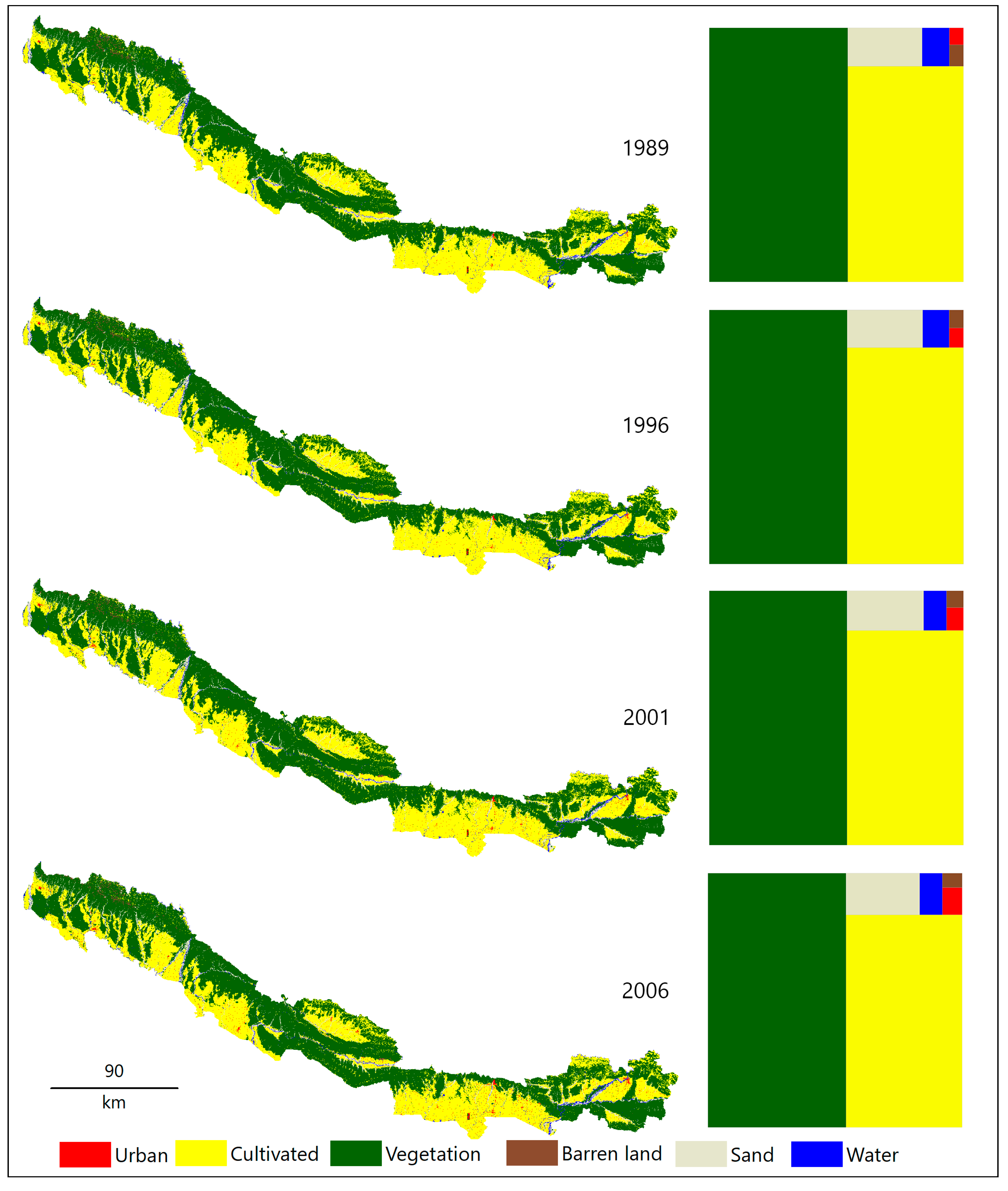
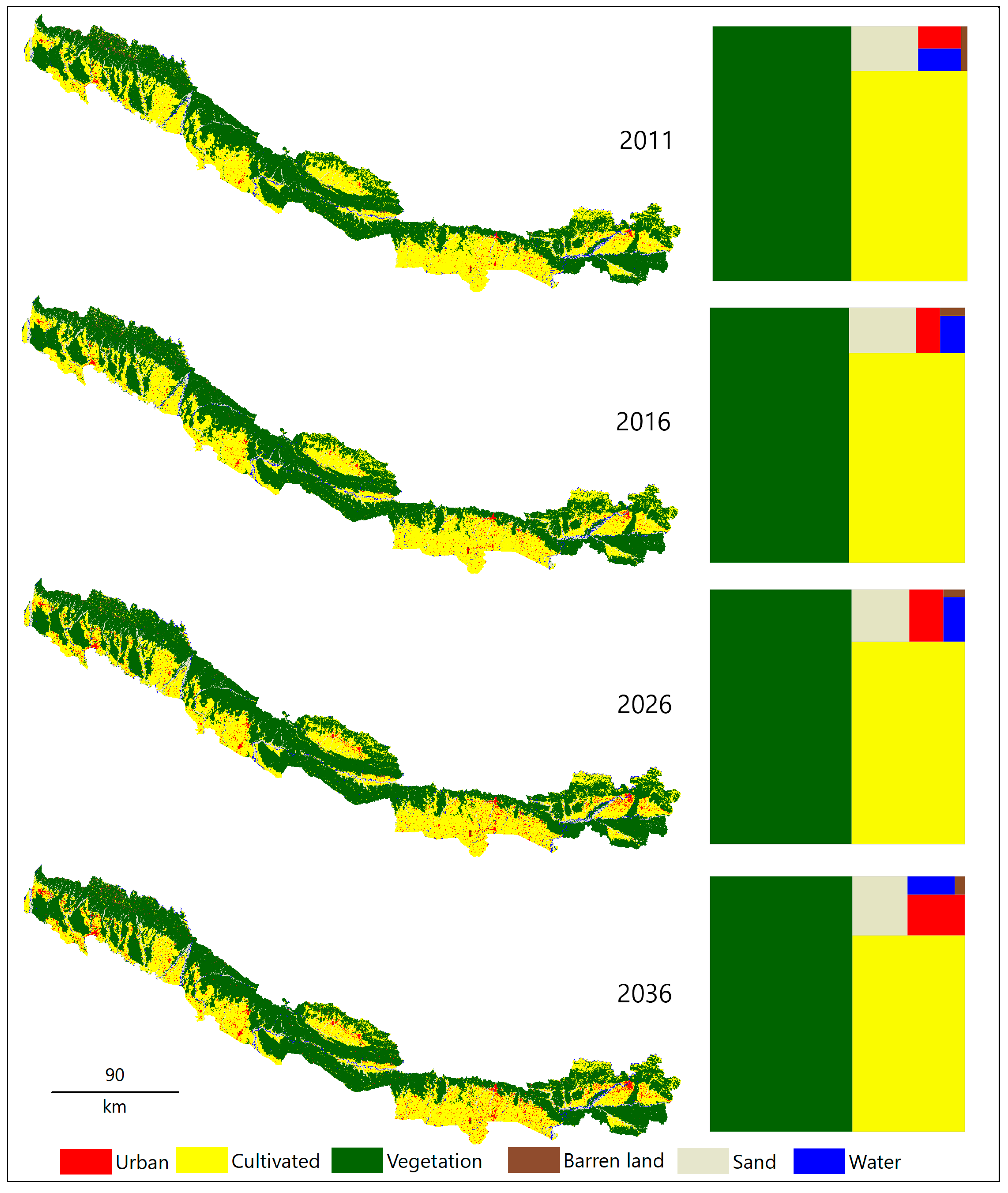
Figure 7.
Land-cover maps from 1989 to 2036, western Tarai region. The sizes of the color-coded boxes at the right are indicative of the relative areas of each land-cover class.
Figure 7.
Land-cover maps from 1989 to 2036, western Tarai region. The sizes of the color-coded boxes at the right are indicative of the relative areas of each land-cover class.


Figure 8.
The figure of merit’s non-nil components (hits, misses, and false alarms) as a percentage of the spatial extent of western Tarai.
Figure 8.
The figure of merit’s non-nil components (hits, misses, and false alarms) as a percentage of the spatial extent of western Tarai.


Table 1.
Cramer’s coefficient for potential factors of land-cover change for model calibration (Bold numbers show the drivers with strong associations used for the LULC modelling).
Table 1.
Cramer’s coefficient for potential factors of land-cover change for model calibration (Bold numbers show the drivers with strong associations used for the LULC modelling).
| Driving Factor | Cramer’s Value |
|---|---|
| Distance to built-up areas | 0.261 |
| Distance to cultivated lands | 0.309 |
| Distance to vegetated areas (forest) | 0.184 |
| Distance to roads | 0.199 |
| Distance to water bodies | 0.078 |
| Elevation | 0.277 |
| Slope | 0.168 |
| Distance to barren lands | 0.081 |
| Distance to sand areas | 0.114 |
Table 2.
Land-use and land-cover (LULC) change over different periods between 1989 and 2016 (in km2).
Table 2.
Land-use and land-cover (LULC) change over different periods between 1989 and 2016 (in km2).
| LULC Classes | 1989–1996 | 1996–2001 | 2001–2006 | 2006–2011 | 2011–2016 | 1989–2016 |
|---|---|---|---|---|---|---|
| Urban/built-up | 11.64 | 32.89 | 44.29 | 119.45 | 47.63 | 255.9 |
| Cultivated land | 67.01 | −53.64 | −97.45 | −115.22 | −50.17 | −249.47 |
| Vegetation cover | −44.54 | −11.5 | 24.84 | 20.09 | 23.88 | 12.77 |
| Barren land | −14.07 | 7.05 | 1.26 | 3.17 | −27.42 | −30.01 |
| Sand cover | −5.53 | 53.18 | 14.42 | −31.31 | 18.56 | 49.32 |
| Water body | −14.51 | −27.98 | 12.64 | 3.82 | −12.48 | −38.51 |
Source: Rimal et al. 2018 [25].
Table 3.
Area of changes during 2016, 2026, and 2036.
| LULC Classes | Area (km2) | Percentage Increase * | ||||
|---|---|---|---|---|---|---|
| 2016 | 2026 | 2036 | 2016–2026 | 2026–2036 | 2016–2036 | |
| Urban/built-up | 327.05 | 526.05 | 691.20 | 60.85 | 31.39 | 111.34 |
| Cultivated land | 7163.65 | 6786.45 | 6508.96 | −5.26 | −4.1 | −9.14 |
| Vegetation cover | 10,472.18 | 10,657.89 | 10,720.12 | 1.77 | 0.58 | 2.37 |
| Barren land | 58.28 | 47.95 | 53.92 | −17.72 | 12.45 | −7.48 |
| Sand cover | 898.55 | 888.67 | 961.13 | −1.1 | 8.15 | 6.96 |
| Water body | 270.07 | 282.59 | 254.27 | 4.64 | −10.0 | −5.85 |
* For a given period, the percentage increase/decrease of a given land cover is expressed in terms of the area of that cover at the beginning of the period in question.
Table 4.
LULC transitions during 2016–2026 (in km2).
| Year | 2026 | |||||||
|---|---|---|---|---|---|---|---|---|
| 2016 | LULC | U/B | CL | VC | BL | SC | WB | Total |
| U/B | 314.93 | 3.06 | 5.97 | 0 | 2.24 | 0.84 | 327.04 | |
| CL | 197.39 | 6591.02 | 310.27 | 0 | 44.15 | 20.82 | 7163.65 | |
| VC | 11.97 | 165.61 | 10,240.43 | 8.63 | 40.05 | 5.48 | 10,472.17 | |
| BL | 0.03 | 0 | 17.7 | 38.58 | 1.64 | 0.26 | 58.21 | |
| SC | 1.66 | 26.75 | 72.49 | 0.39 | 707.11 | 90.14 | 898.54 | |
| WB | 0.06 | 0.02 | 11.02 | 0.34 | 93.48 | 165.05 | 269.97 | |
| Total | 526.04 | 6786.46 | 10,657.88 | 47.94 | 888.67 | 282.59 | 19,189.58 | |
Note: U/B (urban /built-up), CL (cultivated land), VC (vegetation cover), BL (barren land), SC (sand cover), WB (water body).
Table 5.
LULC transitions during 2026–2036 (in km2).
| Year | 2036 | |||||||
|---|---|---|---|---|---|---|---|---|
| 2026 | LULC | U/B | CL | VC | BL | SC | WB | Total |
| U/B | 518.92 | 2.72 | 1.65 | 0 | 2.66 | 0.09 | 526.04 | |
| CL | 156.76 | 6307.74 | 234 | 2.44 | 83.53 | 1.96 | 6786.43 | |
| VC | 12.24 | 162 | 10,424.59 | 11.72 | 39.11 | 7.8 | 10,657.46 | |
| BL | 0 | 0.01 | 9.86 | 37.74 | 0.08 | 0.23 | 47.92 | |
| SC | 1.86 | 19.13 | 35.31 | 1.71 | 743.25 | 87.38 | 888.64 | |
| WB | 1.42 | 16.92 | 14.68 | 0.28 | 92.47 | 156.78 | 282.55 | |
| Total | 691.2 | 6508.52 | 10,720.09 | 53.89 | 961.1 | 254.24 | 19,189.58 | |
Note: U/B (urban /built-up), CL (cultivated land), VC (vegetation cover), BL (barren land), SC (sand cover), WB (water body).
© 2020 by the authors. Licensee MDPI, Basel, Switzerland. This article is an open access article distributed under the terms and conditions of the Creative Commons Attribution (CC BY) license (http://creativecommons.org/licenses/by/4.0/).
Share and Cite
MDPI and ACS Style
Rimal, B.; Sloan, S.; Keshtkar, H.; Sharma, R.; Rijal, S.; Shrestha, U.B. Patterns of Historical and Future Urban Expansion in Nepal. Remote Sens. 2020, 12, 628. https://0-doi-org.brum.beds.ac.uk/10.3390/rs12040628
AMA Style
Rimal B, Sloan S, Keshtkar H, Sharma R, Rijal S, Shrestha UB. Patterns of Historical and Future Urban Expansion in Nepal. Remote Sensing. 2020; 12(4):628. https://0-doi-org.brum.beds.ac.uk/10.3390/rs12040628
Chicago/Turabian StyleRimal, Bhagawat, Sean Sloan, Hamidreza Keshtkar, Roshan Sharma, Sushila Rijal, and Uttam Babu Shrestha. 2020. "Patterns of Historical and Future Urban Expansion in Nepal" Remote Sensing 12, no. 4: 628. https://0-doi-org.brum.beds.ac.uk/10.3390/rs12040628
Note that from the first issue of 2016, this journal uses article numbers instead of page numbers. See further details here.