1. Introduction
In the Digital Cultural Heritage (DCH) domain, the generation of 3D Point Clouds is, nowadays, the more efficient way to manage CH assets. Being a well-established methodology, the representation of CH artifacts through 3D data is a state of art technology to perform several tasks: morphological analysis, map degradation or data enrichment are just some examples of possible ways to exploit such rich informative virtual representation. Management of DCH information is fundamental for better understanding heritage data and for the development of appropriate conservation strategies. An efficient information management strategy should take into consideration three main concepts: segmentation, organization of the hierarchical relationships and semantic enrichment [
1]. Terrestrial Laser Scanning (TLS) and digital photogrammetry allow to generate large amounts of detailed 3D scenes, with geometric information attributes depending on the method used. As well, the development in the last years of technologies such as Mobile Mapping System (MMS) is contributing the massive 3D metric documentation of the built heritage [
2,
3]. Therefore, Point Clouds management, processing and interpretation is gaining importance in the field of geomatics and digital representation. These geometrical structures are becoming progressively mandatory not only for creating multimedia experiences [
4,
5], but also (and mainly) for supporting the 3D modeling process [
6,
7,
8,
9], where even neural networks are lately starting to be employed [
10,
11].
Simultaneously, the recent research trends in HBIM (Historical Building Information Modeling) are aimed at managing multiple and various architectural heritage data [
12,
13,
14], facing the issue of transforming 3D models from a geometrical representation to an enriched and informative data collector [
15]. Achieving such result is not trivial, since HBIM is generally based on scan-to-BIM processes that allow to generate a parametric 3D model from Point Cloud [
16]; these processes, although very reliable since they are made manually by domain experts, have two drawbacks that are noteworthy: first, it is very time consuming and, secondly, it wastes an uncountable amount of data, given that a 3D scanning (both TLS or Close Range Photogrammetry based), contains much more information than the ones required for describing a parametric object. The literature demonstrates that, up to now, traditional methods applied to DCH field still make extensive use of manual operations to capture the real estate from Point Clouds [
17,
18,
19,
20]. Lately, towards this end, a very promising research field is the development of Deep Learning (DL) frameworks for Point Cloud such as Point- Net/Pointnet++ [
21,
22] open up more powerful and efficient ways to handle 3D data [
23]. These methods are designed to recognize Point Clouds. The tasks performed by these frameworks are: Point Cloud classification and segmentation. The Point Cloud classification takes the whole Point Cloud as input and output the category of the input Point Cloud. The segmentation aims at classifying each point to a specific part of the Point Cloud [
24]. Albeit the literature for 3D instance segmentation is limited, if compared to its 2D counterpart (mainly due to the high memory and computational cost required by Convolutional Neural Network (CNN) for scene understanding [
25,
26,
27]), these frameworks may facilitate the recognition of historical architectural elements, at an appropriate level of detail, and thus speeding up the process of reconstruction of geometries in the HBIM environment or in object-oriented software [
28,
29,
30,
31]. To the best of our knowledge, these methods are not applied for the automatic recognition of DCH elements yet. In fact, even if they revealed to be suitable for handling Point Cloud of regular shapes, DCH goods are characterised by complex geometries, highly variable between them and defined only with a high level of detail. In [
19], the authors study the potential offered by DL approaches for the supervised classification of 3D heritage obtaining promising results. However, the work does not cope with the irregular nature of CH data.
To address these drawbacks, we propose a DL framework for Point Cloud segmentation, inspired by the work presented in [
32]. Instead of employing individual points like PointNet [
21], the approach proposed in [
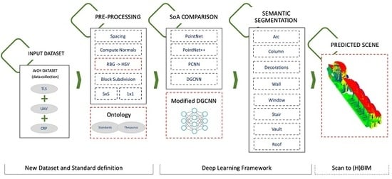
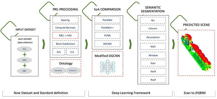
32] exploits local geometric structures by constructing a local neighborhood graph and applying convolution-like operations on the edges connecting neighboring pairs of points. This network has been improved by adding relevant features such as normal and HSV encoded color. The experiments has been performed to a completely new DCH dataset. This dataset comprises 11 labeled points clouds, derived from the union of several single scans or from the integration of the latter with photogrammetric surveys. The involved scenes are both indoor and outdoor, with churches, chapels, cloisters, porticoes and archades covered by a variety of vaults and beared by many different types of columns. They belong to different historical periods and different styles, in order to make the dataset the least possible uniform and homogeneous (in the repetition of the architectural elements) and the results as general as possible. In contrast to many existing datasets, it has been manually labelled by domain experts, thus providing a more precise dataset. We show that the resulting network achieves promising performance in recognizing elements. A comprehensive overall picture of the developed framework is reported in
Figure 1. Moreover, the research community dealing with Point Cloud segmentation can benefit from this work, as it makes available a labelled dataset of DCH elements. As well, the pipeline of work might represent a baseline for further experiments from other researchers dealing with Semantic Segmentation of Point Clouds with DL approaches.
The main contributions of this paper with respect to the state-of-the-art approaches are: (i) a DL framework for DCH semantic segmentation of Point Cloud, useful for the 3D documentation of monuments and sites; (ii) an improved DL approach based on DGCNN with additional Point Cloud features; (iii) a new DCH dataset that is publicly available to the scientific community for testing and comparing different approaches and iv) the definition of a consistent set of architectural element classes, based on the analysis of existing standard classifications.
The paper is organized as follows.
Section 2 provides a description of the approaches that were adopted for Point Clouds semantic segmentation.
Section 3 describes our approach to present a novel DL network operation for learning from Point Clouds, to better capture local geometric features of Point Clouds and a new challenging dataset for the DCH domain.
Section 4 offers an extensive comparative evaluation and a detailed analysis of our approach. Finally,
Section 6 draws conclusions and discuss future directions for this field of research.
3. Materials and Methods
In this section, we introduce the DL framework as well as the dataset used for evaluation. The framework, as said in the introduction section, is depicted in
Figure 1. We use a novel modified DGCNN for Point Cloud semantic segmentation. Further details are given in the following subsections. The framework is comprehensively evaluated on the ArCH Dataset, a publicly available dataset collected for this work.
3.1. ArCH Dataset for Point Cloud Semantic Segmentation
In the state of the art, the most used datasets to train neural networks are: ModelNet 40 [
53] with more than 100k CAD models of objects, mainly furnitures, from 40 different categories; KITTI [
65] that includes camera images and laser scans for autonomous navigation; Sydney Urban Objects [
66] dataset acquired with Velodyne HDL-64E LiDAR in urban environments with 26 classes and 631 individual scans; Semantic3D [
67] with urban scenes as churches, streets, railroad tracks, squares and so on; S3DIS [
68] that includes mainly office areas and it has been collected with the Matterport scanner with 3D structured light sensors and the Oakland 3-D Point Cloud dataset [
69] consisting of labeled laser scanner 3D Point Clouds, collected from a moving platform in a urban environment. Most of the current datasets collect data from urban environments, with scans composed of around 100 K points, and to date there are still no published datasets focusing on immovable cultural assets with an adequate level of detail.
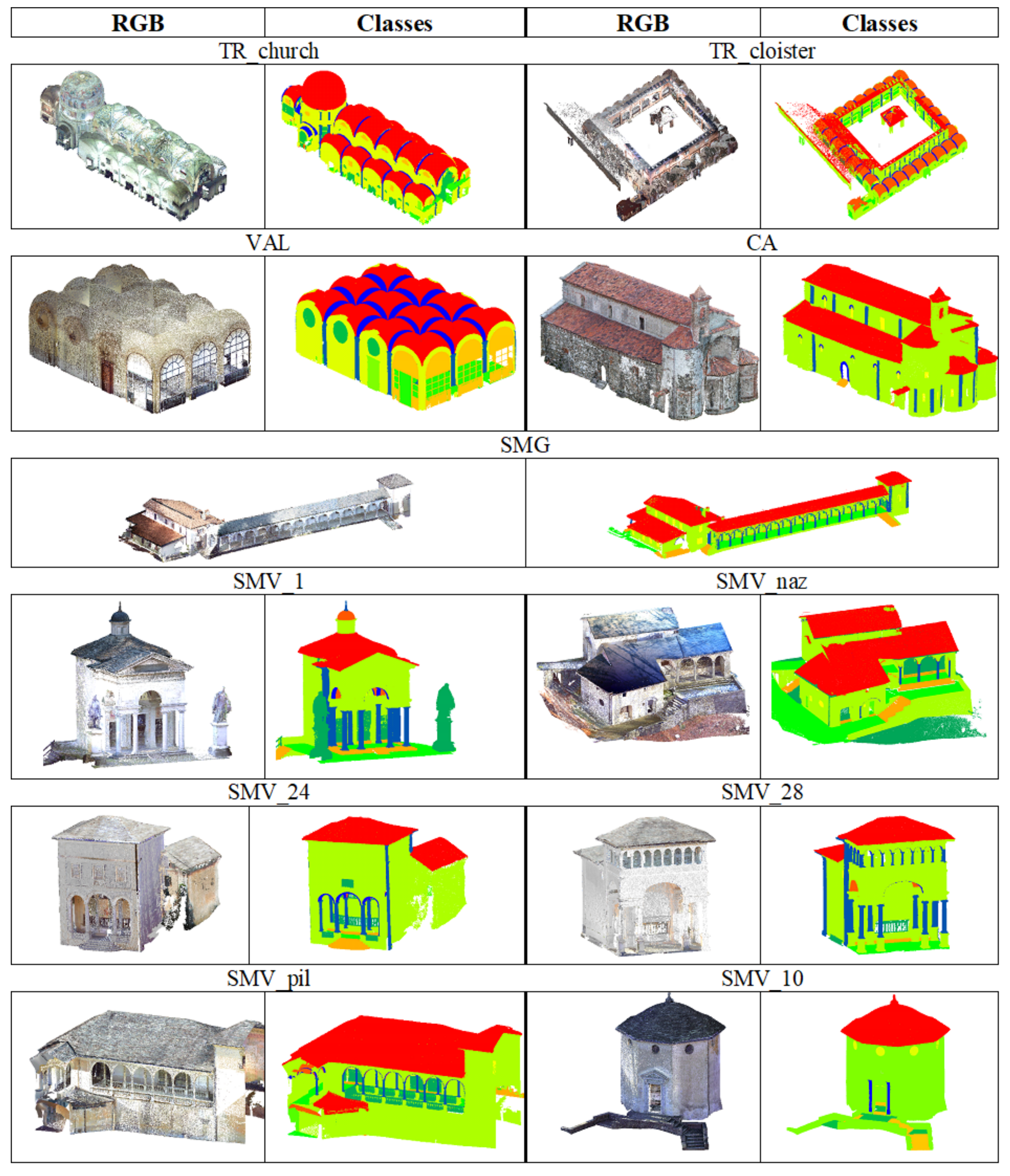
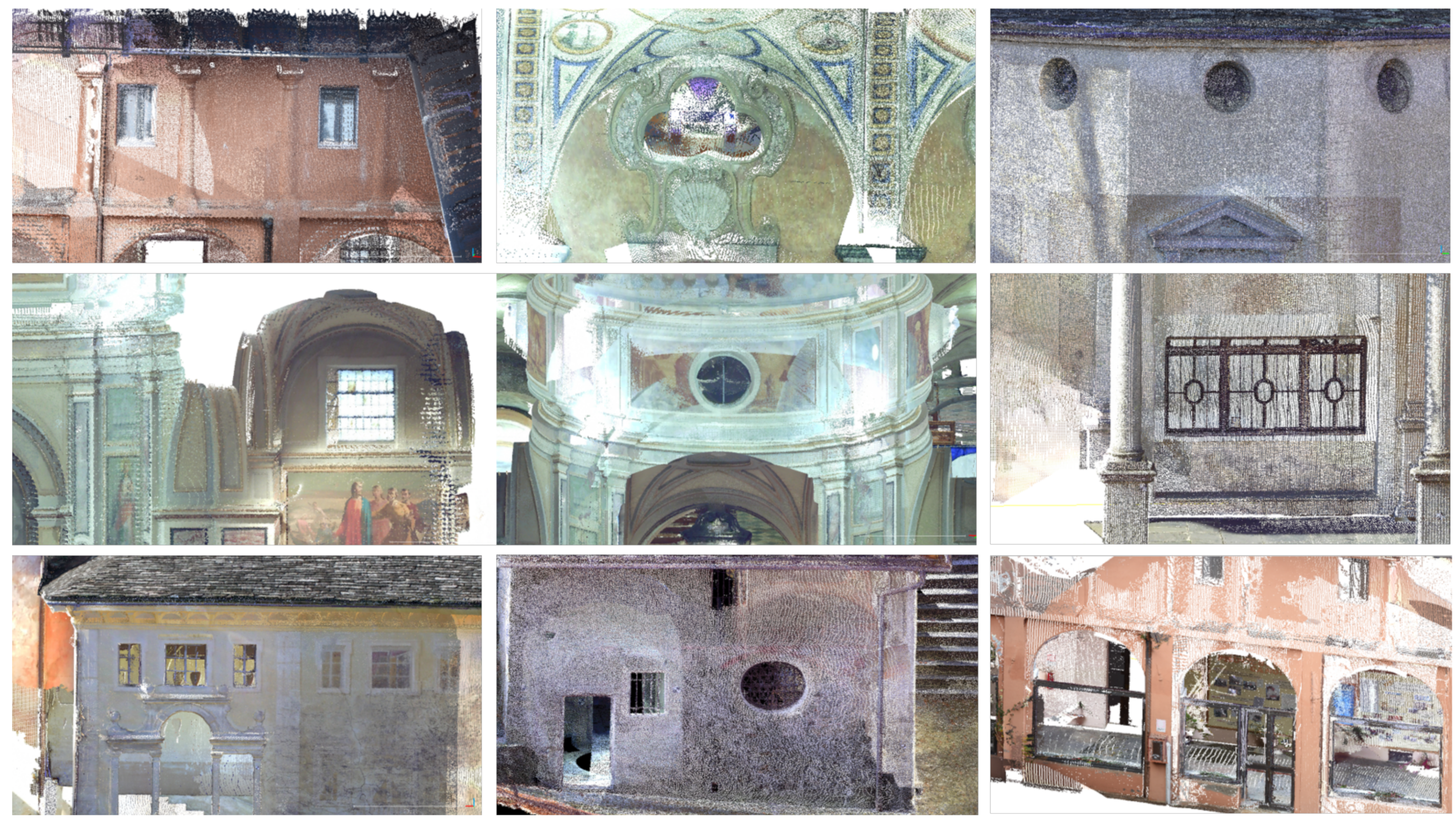
Our proposed dataset, named ArCH (Architectural Cultural Heritage) is composed of 11 labeled scenes (
Figure 2), derived from the union of several single scans or from the integration of the latter with photogrammetric surveys. There are also as many Point Clouds which, however, have not been labeled yet, so they have not been used for the tests presented in this work.
The involved scenes are both indoor and outdoor, with churches, chapels, cloisters, porticoes and archades covered by a variety of vaults and beared by many different types of columns. They belong to different historical periods and different styles, in order to make the dataset the least possible uniform and homogeneous (in the repetition of the architectural elements) and the results as general as possible.
Different case studies are taken into exam and are described as follows: The Sacri Monti (Sacred Mounts) of Ghiffa (SMG) and Varallo (SMV); The Sanctuary of Trompone (TR); The Church of Santo Stefano (CA); The indoor scene of the Castello del Valentino (VA). The ArCH Dataset is publicly available(
http://vrai.dii.univpm.it/content/arch-dataset-point-cloud-semantic-segmentation) for research purposes.
The Sacri Monti (Sacred Mounts) of Ghiffa and Varallo. These two devotional complexes in northern Italy have been included in the UNESCO World Heritage List (WHL) in 2003. In the case of the Sacro Monte di Ghiffa, a 30 m loggia with tuscanic stone columns and half pilasters has been chosen; while for the Sacro Monte of Varallo 6 buildings have been included in the dataset, containing a total of 16 chapels, some of which very complex from an architectural point of view: barrel vaults, sometimes with lunettes, cross vaults, arcades, balustrades and so on.
The Sanctuary of Trompone (TR). This is a wide complex dating back to the 16th century and it consists of a church (about 40 × 10 m) and a cloister (about 25 × 25 m), both included in the dataset. The internal structure of the church is composed of 3 naves covered by cross vaults supported in turn by stone columns. There is also a wide dome at the apse and a series of half-pilasters covering the sidewalls.
The Church of Santo Stefano (CA) has a completely different compositional structure if compared with the previous one, being a small rural church from the 11th century. There is a stone masonry, not plastered, brick arches above the small windows and a series of Lombard band defining a decorated moulding under the tiled roof.
The indoor scene of the Castello del Valentino (VA) is a courtly room part of an historical building recast from the 17th century. This hall is covered by cross vaults leaning on six sturdy breccia columns. Wide French windows illuminate the room and oval niches surrounded by decorative stuccoes are placed on the sidewalls. This case study is part of a serial site inserted in the WHL. of UNESCO in 1997.
In the majority of cases, the final scene was obtained through the integration of different Point Clouds, those acquired with the terrestrial laser scanner (TLS), and those deriving from photogrammetry (mainly aerial for surveying the roofs), after appropriate evaluation of the accuracy. This integration results in a complete Point Cloud, with different density according to the sensors used, however leading to increasing the overall Point Cloud size and requiring a pre-processing phase for the NN.
The common structure of the Point Clouds is therefore based on the sequence of the coordinates x, y, z and the R, G, B values.
In the future, other point clouds will be added to the ArCH dataset, to improve the representation of complex CH objects with the potential contribution of all the other researchers involved in this field.
3.2. Data Pre-Processing
To prepare the dataset for the network, pre-processing operations have been carried out in order to make the cloud structures more homogeneous. The pre-processing methods, for this dataset, have followed 3 steps: translation, subsampling and choice of features.
The spatial translation of the Point Clouds is necessary because of the georeferencing of the scenes, the coordinate values are in fact too large to be processed by the deep network, so the coordinates are truncated and each single scene is spatially moved close to the point cardinal (0,0,0). This operation on the one hand has led to the loss of georeferencing, on the other hand, however, it has made possible to reduce the size of the files and the space to be analyzed, thus also leading to a decrease in the required computational power.
The subsampling operation, which became necessary due to the high number of points (mostly redundant) present in each scene (>20 M points), was instead more complex. It was in fact necessary to establish which of the three different subsampling options was the most adequate to provide the best typology of input data to the neural network. The option of random subsampling was discarded because it would limit the test repeatability, then both the other two methods have been tested: octree and space. The first is efficient for nearest neighbor extraction, while the second provides, in the output Point Cloud, points not closer than the distance specified. As far as space is concerned, it has been set a minimum space between points of 0.01 m, in this way a high level of detail is ensured, but at the same time it is possible to considerably reduce the number of points and the size of the file, in addition to regularize the geometric structure of the Point Cloud
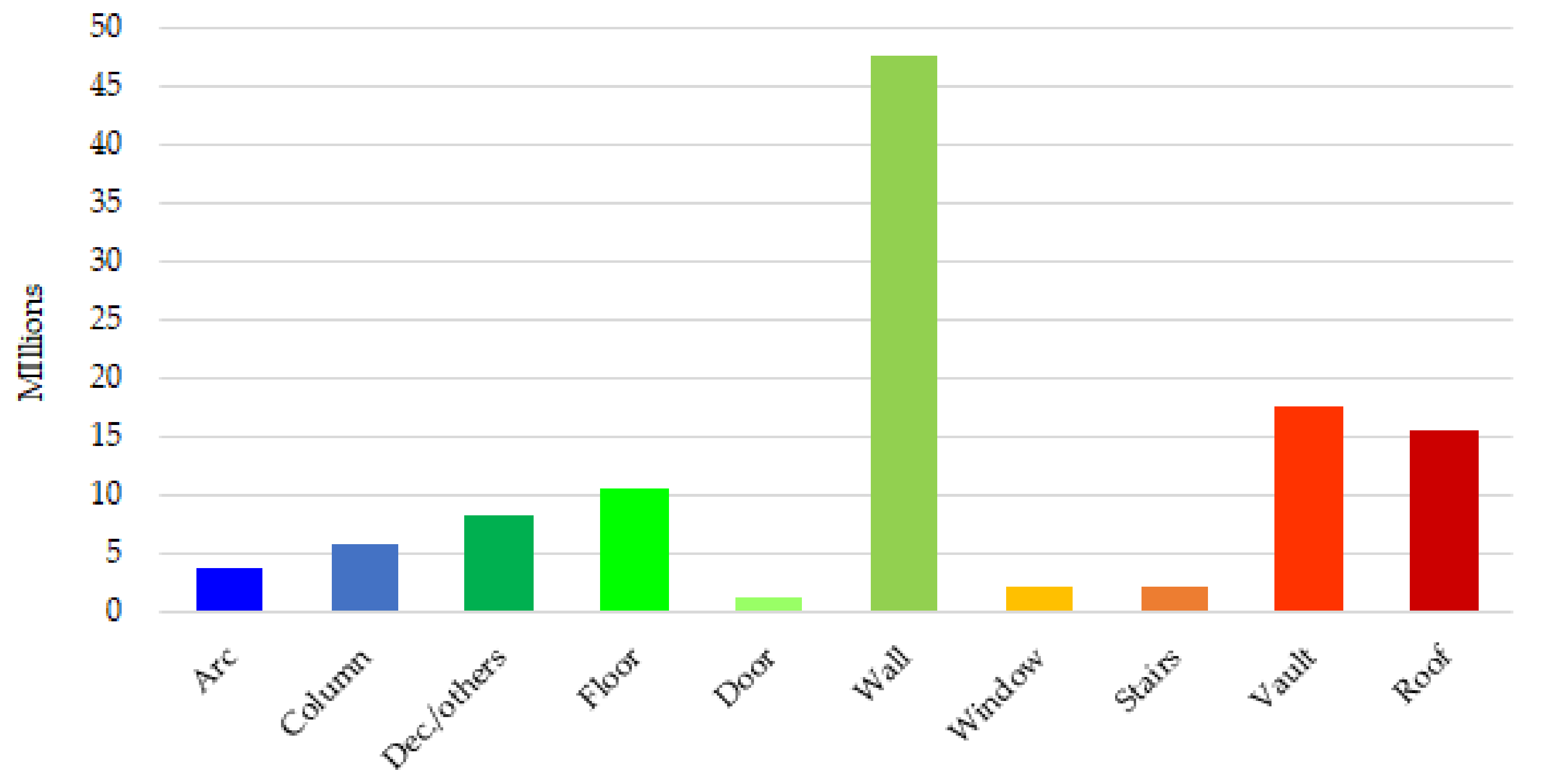
As for the octree, applied only in the first tests on half of the Trompone Church scene, level 20 was set, so that the number of final points was more or less similar to that of the scene subsampled with the space method. The software used for this operation is CloudCompare. An analysis of the number of points for each scene is detailed in
Table 1, where it is possible to see the lack of points for some classes and the highest total value for the ‘Wall’ class.
The
extraction of features directly from the Point Clouds is instead an open and constantly evolving field of research. Most of the features are handcrafted for specific tasks and can be subdivided and classified into intrinsic and extrinsic, or also used for local and global descriptors [
40,
70]. The local features define statistical properties of the local neighborhood geometric information, while the global features describe the whole geometry of the Point Cloud. Those mostly used are the local ones, such as eigenvalues based descriptors, 3D Shape context and so on, however in our case, since the last networks developed [
22,
32] tend to let the network itself learn the features and since our main goal is to generalize as much as possible, in addition to reduce the human involvement in the pre-proccessing phases, the only features calculated are the normals and the curvature. The normals are calculated on Cloud Compare and have been computed and orientated with different settings depending on the surface model and 3D data acquisition. Specifically a plane or quadric ‘local surface model’ as surface approximation for the normals computation has been used and a ‘minimum spanning tree’ with Knn = 10 has been set for their orientation. The latter has been further checked on MATLAB
®.
3.3. Deep Learning for Point Cloud Semantic Segmentation
State-of-the-art deep neural networks are specifically designed to deal with the irregularity of Point Clouds, directly managing raw Point Cloud data rather than using an intermediate regular representation. In this contribution, the performances obtained with the ArCH dataset of some state-of-art architectures are therefore compared and then evaluated with regards to the DGCNN we have modified. The NNs selected are:
PointNet [
21], as it was the pioneer of this approach, obtaining permutation invariance of points by operating on each point independently and applying a symmetric function to accumulate features.
its extensions
PointNet++ [
22] that analyzes neighborhoods of points in preference of acting on each separately, allowing the exploitation of local features even if with still some important limitations.
PCNN [
71], a DL framework for applying CNN to Point Clouds generalizing image CNNs. The extension and restriction operators are involved, permitting the use of volumetric functions associated to the Point Cloud.
DGCNN [
32] that addresses these shortcomings by adding the EdgeConv operation. EdgeConv is a module that creates edge features describing the relationships between a point and its neighbors rather than generating point features directly from their embeddings. This module is permutation invariant and it is able to group points thanks to local graph, learning from the edges that link points.
3.4. DGCNN for DCH Point Cloud Dataset
In our experiments, we build upon the DGCNN implementation provided by [
32]. Such an implementation of DGCNN uses k-nearest neighbors (kNN) to individuate the
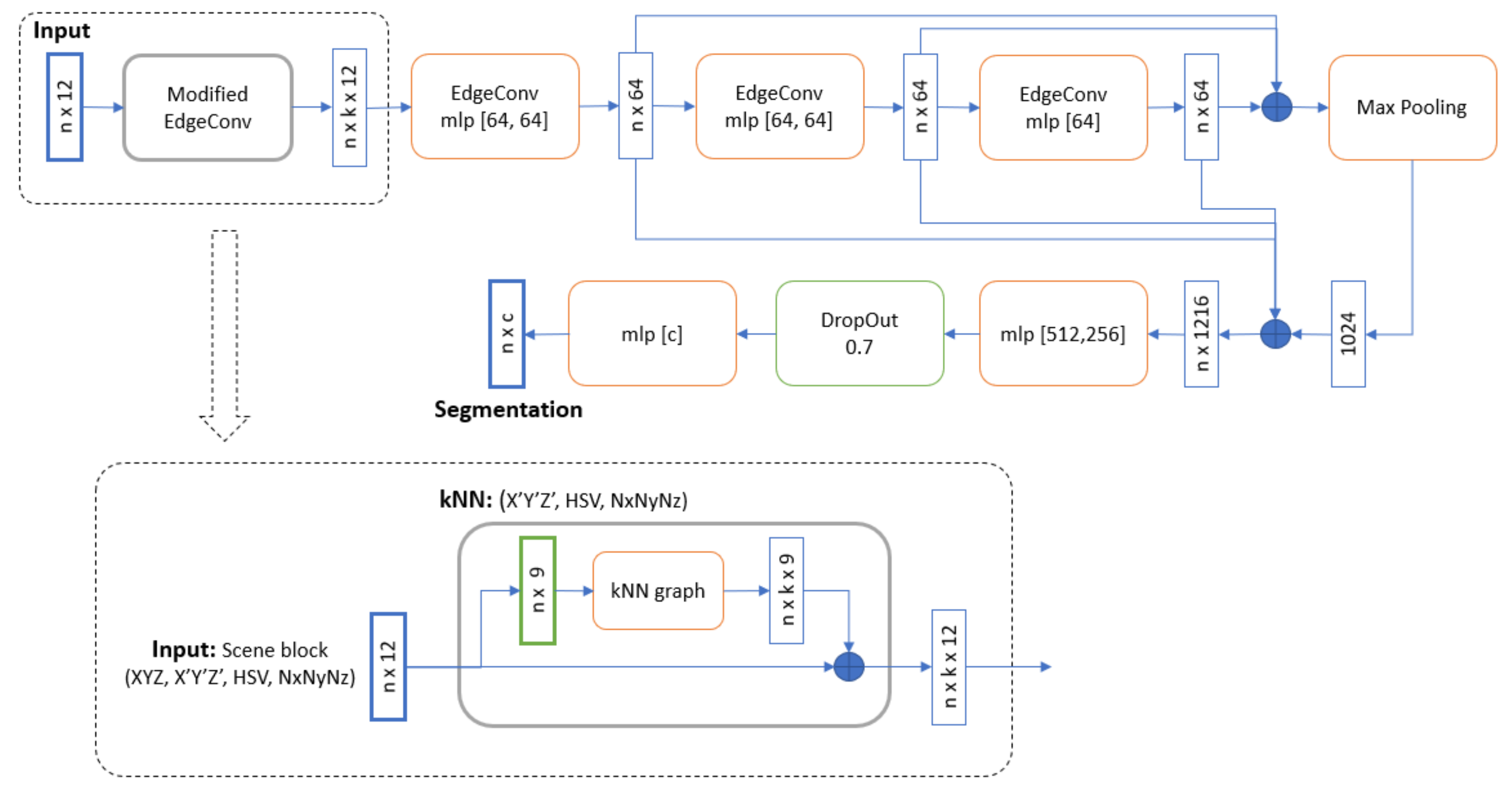
k points closest to the point to be classified, thus defining the neighboring region of the point. The edge features are then calculated from such a neighboring region and provided as input to the following layer of the network. Such a edge convolution operation is performed on the output of each layer of the network. In the original implementation, at the input layer kNN is fed with normalized points coordinates only, while in our implementation we use all the available features. Specifically, we added color features, expressed as RGB or HSV, and normal vectors.
Figure 3 shows the overall structure of the network. We give in input a scene block, composed of 12 features for each point: XYZ coords, X’Y’Z’ normalized coords, color features (HSV channels), normals features. These blocks pass through 4 EdgeConv layers and a max-pooling layer to extract global features of the block. The original XYZ coordinates are kept to take into account the positioning of the points in the whole scene, while the normalized coordinates represent the positioning within each block. The KNN module is fed with normalized coordinates only and both original and normalized coordinates are used as input features for the neural network. RGB channels have been converted to HSV channels in two steps: first they are normalized to values between 0 and 1, then they are converted to HSV channels using the rgb2hsv() function of the scikit-image library implemented in python. This conversion is useful because the individual channels H, S and V are independent one from the other, each of them has a different typology information, making them independent features. Channels R, G and B are conversely somehow related to each other, they share a part of the same data type, so they should not be used separately.
The choice of using normals and HSV is based on different reasons. On one side the RGB component, based on the sensors used in data acquisition, is most of the time present as a property of the point cloud and therefore it has been decided to fully exploit this kind of data; on the other the RGB components define the radiometric properties of the point cloud, while the normals define some geometric properties. In this way we are using as input for the NN different kinds of information. Moreover, the decision to convert the RGB into HSV is borrowed from other research works [
72] that, even if developed for different tasks, show the effectiveness of this operation.
We have therefore tried to support the NN, in order to increase the accuracy, with few common features that could be easily obtained by any user.
These features are then concatenated with the local features of each EdgeConv. We have modified the first EdgeConv layer so that the kNN could also use color and normal features to be able to select k neighbors for each point. Finally, through 3 convolutional layers and a dropout layer, we will output the same block of points but with segmentation scores (one for each class to be recognized). The output of the segmentation will be given by the class with the largest score.
4. Results
In this section, the results of the experiments conducted on “ArCH Dataset” are reported. In addition to the performance of our modified DGCNN, we also present the performance of PointNet [
21], PointNet++ [
22], PCNN [
71] and DGCNN [
32] which form the basis of the improvement of our network.
Our experiments are separated in two phases. In the first one, we attempt at tuning the networks, choosing the best parameters for the task of semantically segmenting our ArCH dataset. To this end we have considered a single scene and used an annotated portion of it for training the network, evaluating the performances on the remaining portion of the scene. We have chosen to perform such first experiments on the TR_church (Trompone) as it presents a relatively high symmetry, allowing us to subdivide it in parts with similar characteristics, and it includes almost all the considered classes (9 out of the 10). Such an experimental setting addresses the problem of automatically annotating a scene that has been only partially annotated manually. While this has in fact practical applications, and could speed up the process of annotating an entire scene, our goal is to evaluate the automatic annotation of an scene that was never seen before. We address this more challenging problem, in the second experimental phase, where we train the networks with 10 different scenes and then attempt at automatically segmenting the remaining one. Segmentation of the entire Point Cloud into sub-parts (blocks) is a needed pre-processing step for all the analysed neural architectures. For each block a fixed number of points have to be sampled. This is due to the fact that neural networks need a constant number of points as input and that it would be computationally unfeasible to provide all the points at once to the networks.
4.1. Segmentation of Partially Annotated Scene
Two different settings have been evaluated in this phase: a k-fold cross-validation and a single splitting of the labeled dataset into a training set and a test set. In the first case the overall number of test samples is small and the network is trained on more samples. In the second case, an equal number of samples is used to train and to evaluate the network, possibly leading to very different results. This, for completeness, we experimented with both settings.
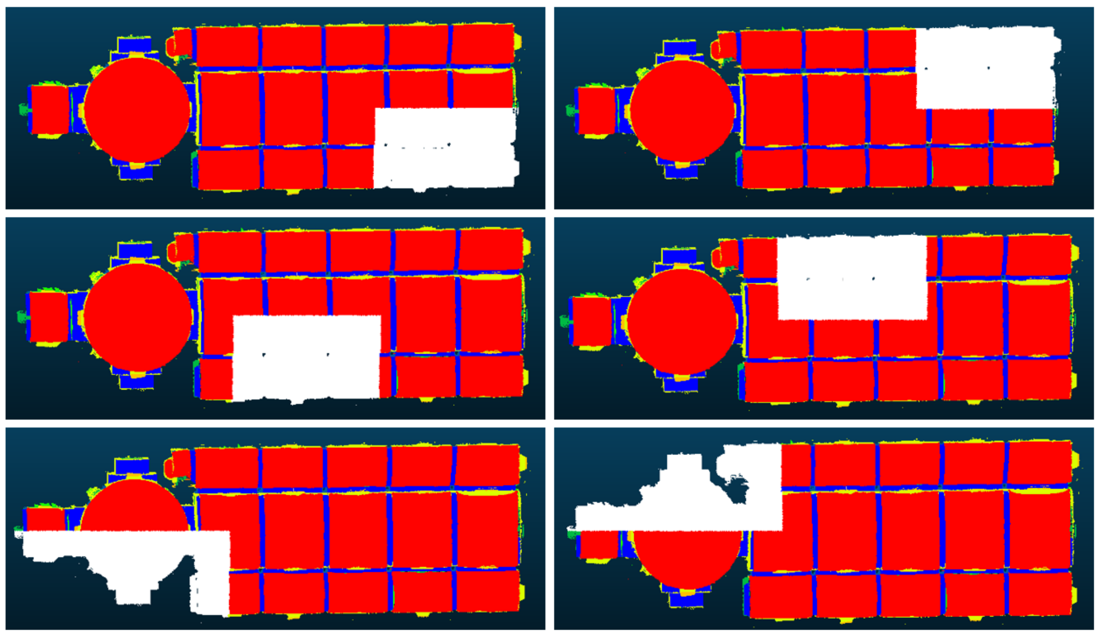
In the first setting, the TR_church scene was divided into 6 parts and we have performed a cross-validation with 6 Fold, as shown in
Figure 4. We have tested different combinations of hyperparameters of the various networks to be able to verify which was the best, as we can see in
Table 2, where the mean accuracy is derived from calculating the accuracy of each test (fold), then averaging them.
Regarding the pointcloud preprocessing steps, which consists in segmenting the whole scene into blocks and, for each block, sampling a number of points, we used, for each evaluated model, the settings used in the corresponding original paper. PointNet and PointNet++ use blocks are of size meters and 4096 points for cloud sampling. In the case of the DGCNN, we have used blocks of size and 4096 points per block. Finally, the PCNN network was tested using the same sampling as the DGCNN (), but using 2048 points, as this is the default setting used in the PCNN paper. We also tested PCNN providing 4096 points per block, but results were slightly worse. We also notice that the performances improve slightly using the color features represented as HSV color-map. The HSV (hue, saturation, value) representation is known for more closely aligning with the human perception of colors and, by representing colors as three independent variables, allows, for example, to take into account variations, e.g., due to shadows and different light conditions.
In the second setting, we have split the TR-cloister scene in half, choosing the left side for the training and the right side for the test. Furthermore, we split the left side into a training set (80%) and a validation set (20%). We used the validation set to test overall accuracy at the end of each training epoch and we performed evaluation on the test set (right side). In
Table 3, the performance of state-of-the-art networks are reported. We report results obtained with the hyperparameters combinations that best performed in the cross-validation experiment.
Table 4 shows the metrics in the test phase for each class of the Trompone’s right side. In this table we report, for each class, precision, recall, F-1 score and Intersection over Union (IoU). This table allows us to understand which are the classes that are best discriminated by the various approaches, to understand which are their weak points and their strengths (as broadly discussed in
Section 5).
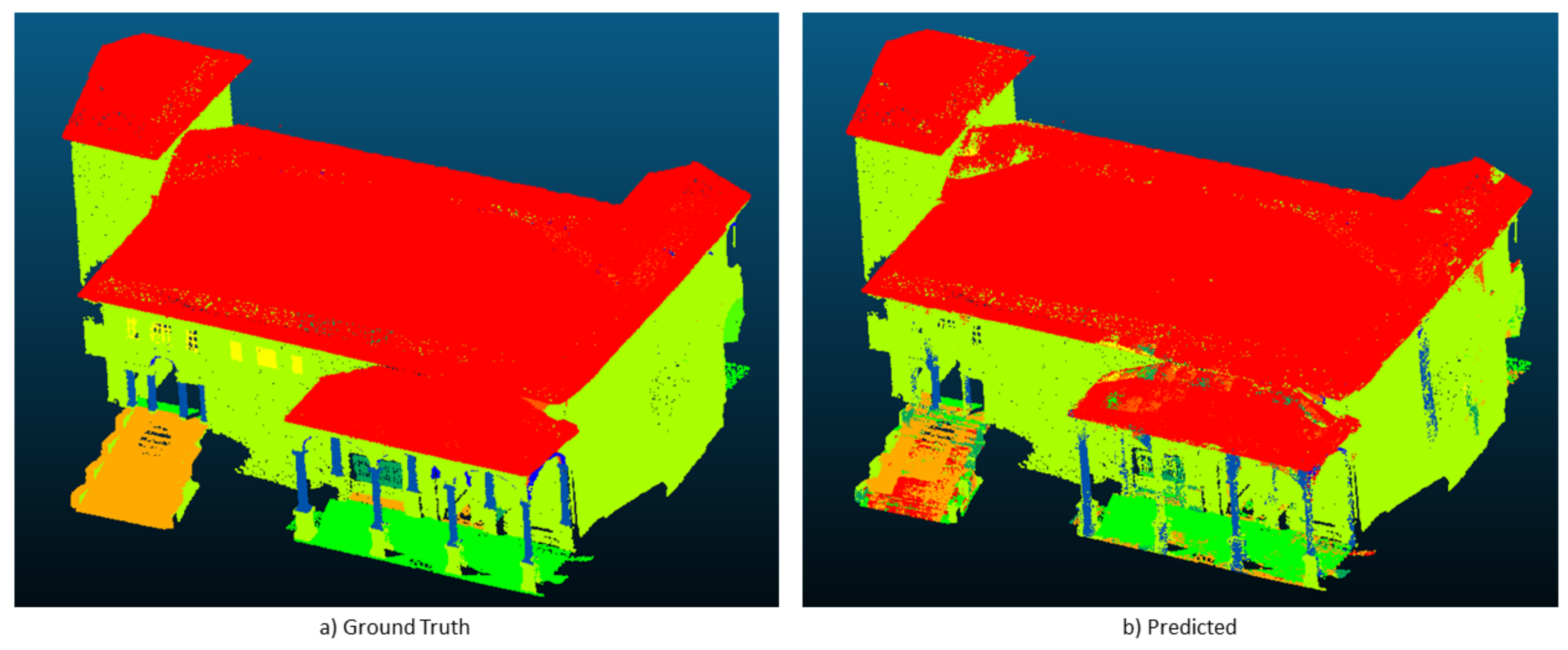
Finally,
Figure 5 depicts the manually annotated test scene (ground truth) and the automatic segmentation results obtained with our approach.
4.2. Segmentation of an Unseen Scene
In the second experimental phase, we used all the scenes of ArCH Dataset: 9 scenes were used for the Training, 1 scene as Validation (Ghiffa scene), 1 scene for the Final Test (SMV). State-of-the-art networks were evaluated, comparing the results with our DGCNN-based approach. In
Table 5, the overall performances are reported for each tested model, while in
Table 6 reports detailed results on the individual classes of the test scene.
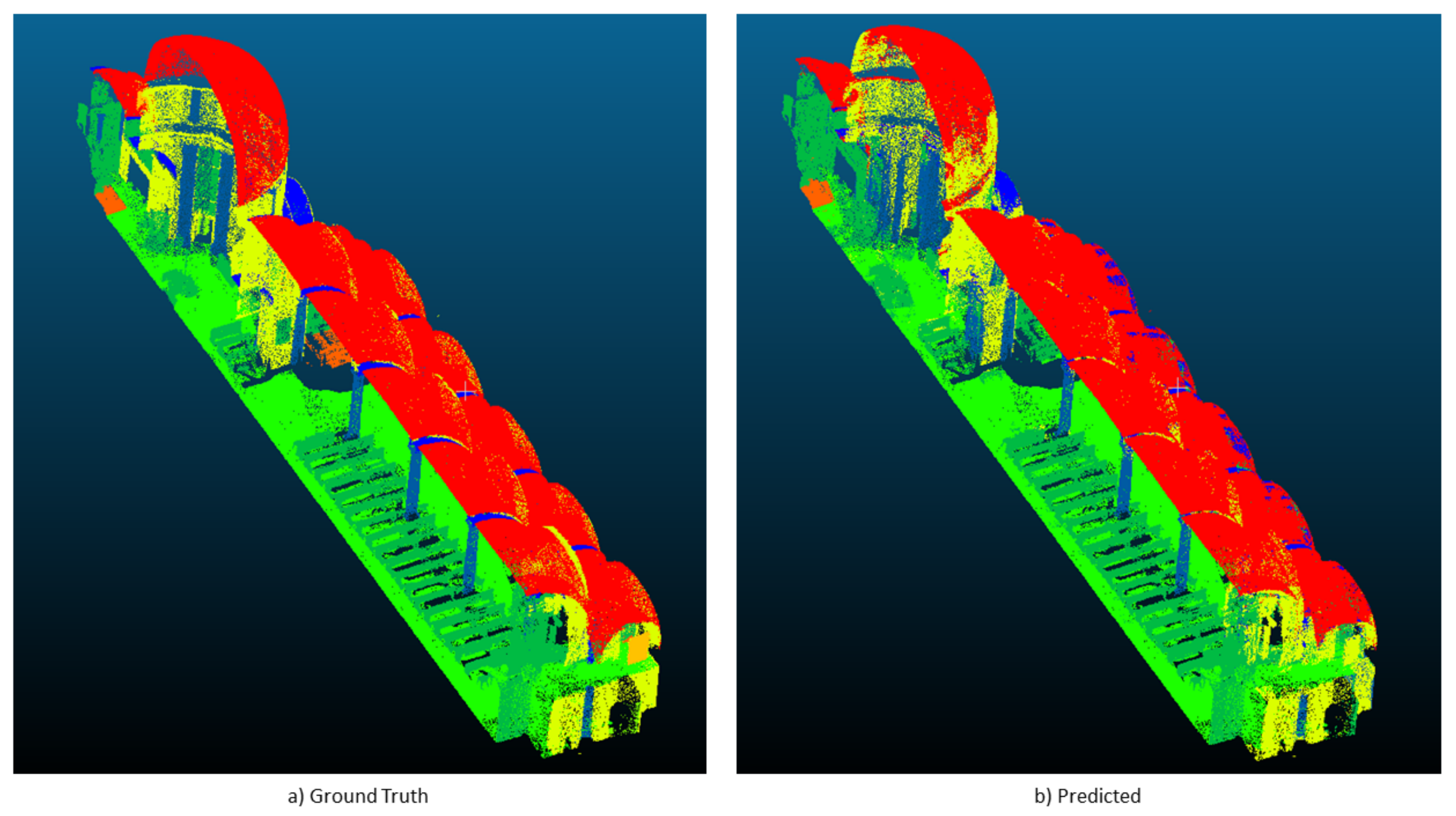
Figure 6 and
Figure 7 depict the confusion matrix and the segmentation results of the last experiment: 9 scenes for Training, 1 scene for validation and 1 scene for test.
The performance gain provided by our approach is more evident than in previous experiments, leading to an improvement of around 0.8 in overall accuracy as well as in F1-score. The IoU also increases. In
Table 6, one can see that our approach outperforms the others in the segmentation of almost all classes. For some classes values of Precision and Recall are lower than the original DGCNN. However, our modified DGCNN generally improves performance in terms of F1-score. This metric is a combination of Precision and Recall, thus it allows to better understand how the network is learning.
5. Discussion
This research rises remarkable research directions (and challenges) that is worth to deepen. First of all, looking at the first experimental setting, performances are worse than those obtained in the K-fold experiment (referring to
Table 3). This is probably do to the fact that the network has less points to learn on. As in the previous experiment, the results on the test set is obtained with our approach, confirming that HSV and Normals does in fact help the network to learn higher level features of the different classes. Besides, as reported in
Table 4 and confirmed in
Figure 5, we can notice that using our setting helps in detecting
vaults, increasing precision, recall and IoU, as well as
columns and
stairs, by sensibly increasing recall and IoU.
Dealing with the second experimental setting (see
Section 4.2), it is worth to notice that all evaluated approaches fail in recognizing classes with low support, as
doors,
windows and
arcs. Beside, for these classes we observe a high variability in shapes across the dataset, this probably contributes to the bad accuracy obtained by the networks.
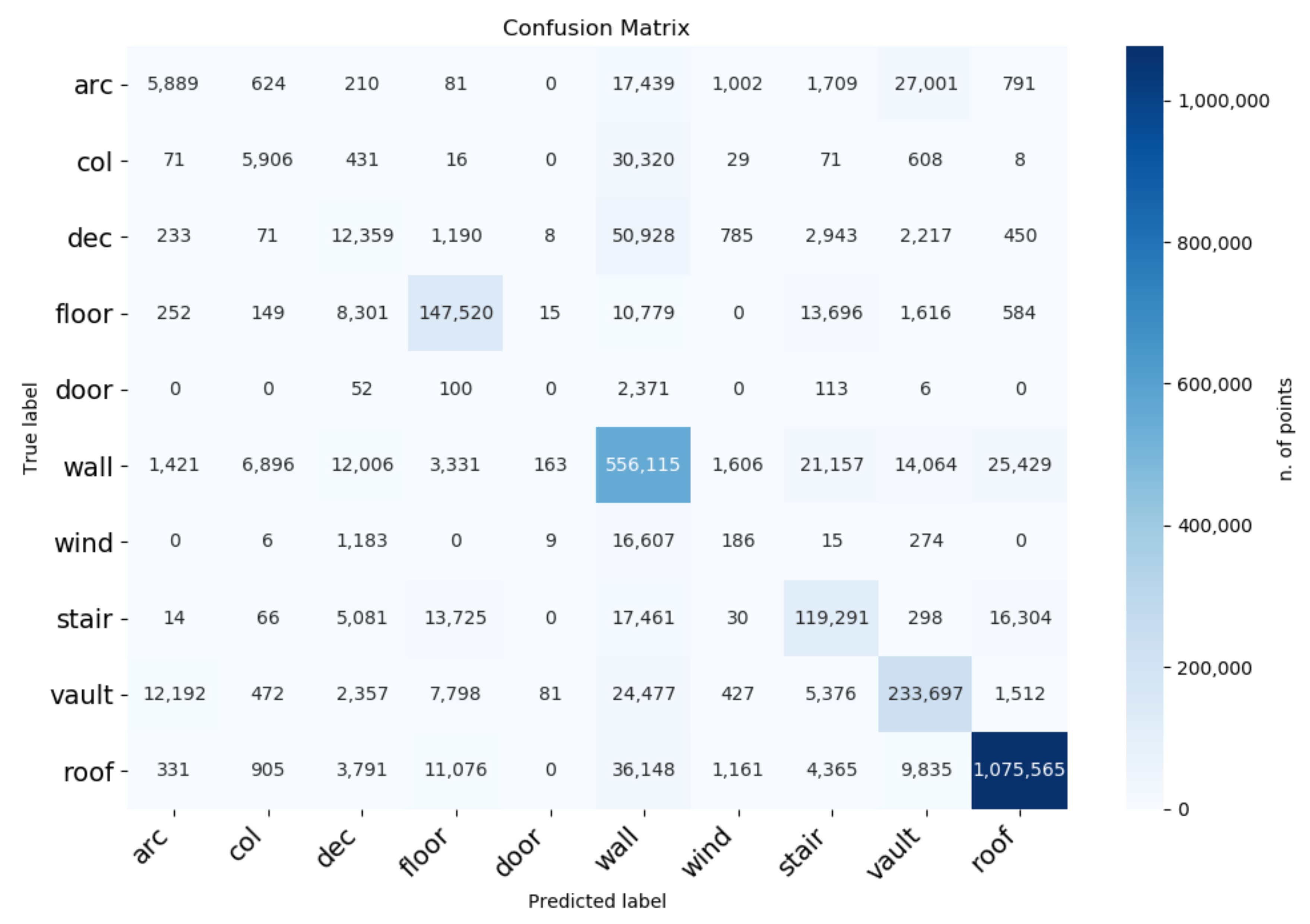
More insights can be drawn from the confusion matrix, shown in
Figure 6. It reveals, for example, that
arcs are often confused with
vaults, as they clearly share geometrical features, while
columns are often confused with
walls. The latter behaviour can be possibly due to the presence of half-pilasters, which are labeled as columns but have a shape similar to walls. The unbalanced nature of the number of points per class is clearly highlighted in
Figure 8.
Furthermore, if we consider the classes individually, we can see that the lowest values are in Arc, Dec, Door and Window. More in detail:
Arc: the geometry of the elements of this class is very similar to that of the vaults and, although the dimensions of the arcs are not similar to the latter, most of the time they are really close to the vaults, almost a continuation of these elements. For these reasons the result is partly justifiable and could lead to the merging of these two classes.
Dec: in this class, which can also be defined as “Others” or “Unassigned”, all the elements that are not part of the other classes (such as benches, paintings, confessionals…) are included. Therefore it is not fully considered among the results.
Door: the null result is almost certainly due to the very low number of points present in this class (
Figure 8). This is due to the fact that, in the proposed case studies of CH, it is more common to find large arches that mark the passage from one space to another and the doors are barely present. In addition, many times, the doors were open or with occlusions, generating a partial view and acquisition of these elements.
Window: in this case the result is not due to the low number of windows present in the case study, but to the high heterogeneity between them. In fact, although the number of points in this class is greater, the shapes of the openings are very different from each other (three-foiled, circular, elliptical, square and rectangular) (
Figure 9). Moreover, being mostly composed of glazed surfaces, these surfaces are not detected by the sensors involved such as the TLS, therefore, unlike the use of images, in this case the number of points useful to describe these elements is reduced.
6. Conclusions
The semantic segmentation of Point Clouds is a relevant task in DCH as it allows to automatically recognise different types of historical architectural elements, thus possibly saving time and speeding up the process of analysing Point Clouds acquired on-site and building parametric 3D representations. In the context of historical buildings, Point Cloud semantic segmentation is made particularly challenging by the complexity and high variability of the objects to be detected. In this paper, we provide a first assessment of state-of-the-art DL based Point Cloud segmentation techniques in the Historical Building context. Beside comparing the performances of existing approaches on ArCH (Architectural Cultural Heritage), created on purpose and released to the research community, we propose an improvement which increase the segmentation accuracy, demonstrating the effectiveness and suitability of our approach. Our DL framweork is based on a modified version of DGCNN and it has been applied to a newly puclic collected dataset: ArCH (Architectural Cultural Heritage). Results prove that the proposed methodology is suitable for Point Cloud semantic segmentation with relevant applications. The proposed research starts from the idea of collecting relevant DCH dataset which is shared together with the framework source codes to ensure comparisons with the proposed method and future improvements and collaborations over this challenging problems. The paper describes one of the more extensive test based on DCH data, and it has huge potential in the field of HBIM, in order to make the scan-to-BIM process affordable.
However, the developed framework highlighted some shortcomings and open challenges that is fair to mention. First of all, the framework is not able to assess the accuracy performances with respect to the acquisition techniques. In other words, we seek to uncover, in future experiments, if the adoption of Point Clouds acquired with other methods changes the DL framework performances. Moreover, as stated in the results section, the dimensions of points per classes is unbalanced and not homogeneous, with the consequent biases in the confusion matrix. This bottleneck could be solved by labelling a more detailed dataset or creating synthetic Point Clouds. The research group is focusing his efforts even in this direction [
73]. In future works, we plan to improve and better integrate the framework with more effective architectures, in order to improve performances and test also different kind of input features [
19,
74].

 ,
, 


