Point Cloud vs. Mesh Features for Building Interior Classification


1
Department of Civil Engineering, TC Construction—Geomatics, KU Leuven—Faculty of Engineering Technology, 9000 Ghent, Belgium
2
Geomatics Unit, University of Liège, 4000 Liège, Belgium
*
Author to whom correspondence should be addressed.
Remote Sens. 2020, 12(14), 2224; https://0-doi-org.brum.beds.ac.uk/10.3390/rs12142224
Submission received: 4 June 2020
/
Revised: 30 June 2020
/
Accepted: 6 July 2020
/
Published: 11 July 2020
(This article belongs to the Special Issue Point Cloud Processing and Analysis in Remote Sensing)
Abstract
:Interpreting 3D point cloud data of the interior and exterior of buildings is essential for automated navigation, interaction and 3D reconstruction. However, the direct exploitation of the geometry is challenging due to inherent obstacles such as noise, occlusions, sparsity or variance in the density. Alternatively, 3D mesh geometries derived from point clouds benefit from preprocessing routines that can surmount these obstacles and potentially result in more refined geometry and topology descriptions. In this article, we provide a rigorous comparison of both geometries for scene interpretation. We present an empirical study on the suitability of both geometries for the feature extraction and classification. More specifically, we study the impact for the retrieval of structural building components in a realistic environment which is a major endeavor in Building Information Modeling (BIM) reconstruction. The study runs on segment-based structuration of both geometries and shows that both achieve recognition rates over 75% F1 score when suitable features are used.
1. Introduction
The automated interpretation of building environments is a major topic in the current literature [1]. Where modelers used to manually identify building components such as structural elements and furniture, more unsupervised workflows are proposed for scene interpretation [2]. Applications such as Scan-to-BIM and indoor navigation of autonomous robots heavily rely on rapid scene interpretation, making its automation highly desired by the industry [3].
The interpretation of building environments is typically performed on a set of observations such as imagery or point clouds. From these inputs, a set of relevant features is extracted which is then used to classify the observations [4]. Generally, structural elements such as walls and slabs are identified first after which domain-specific components are detected. Also, because structural elements have more distinct geometry than visual characteristics, the classification is typically performed on the metric data [5]. Currently, researchers have nearly exclusively worked on point cloud data acquired from Terrestrial Laser Scanning (TLS), Indoor Mobile Mapping Systems (IMMS) or RGBD sensors [6]. However, researchers have reported that the noise, occlusions, uneven data distribution and sparsity of point clouds can lead to severe misclassifications [4,7,8]. Alternatively, mesh geometry is becoming more accessible for building geometry due to the recent advancements in speed, correctness and detailing of meshing operations [9]. Meshes are not hindered by the above obstacles in point cloud data and thus could potentially improve the detection rate [10]. However, researchers typically generate features from their raw input data and overlook the geometry representation opportunities despite their obvious impact on the feature extraction. As a result, there currently is a gap in the literature investigating the impact of geometry representations on the feature extraction in building environments. The few research papers that do actually compare features mostly focus on the impact of features on the result without considering the geometry representation [11,12,13]. In this research, we specifically target the comparison of mesh segments to point cloud segments, providing a much-needed empirical study for building interpretation. We extend on the unsupervised segmentation frameworks proposed in [14,15] for both point cloud and 3D mesh geometries. In summary, the method’s main contributions are:
- A theoretical comparison between mesh-based and point-based geometries for classification
- An empirical study that compares both approaches in terms of feature discriminativeness, distinctness and classification results
- An implementation of frequently used building classification features and the validation on the Stanford 2D-3D-Semantics Dataset (2D-3D-S).
The remainder of this work is structured as follows. The background and related work is presented in Section 2. In Section 3 we propose a methodology for extracting pertinent features designed for efficient classification. The workbench design and experimental results are given in Section 4 and discussed in Section 5 and Section 6. Finally, major conclusions are presented in Section 7.
2. Background and Related Work
The typical procedure to interpret building geometry is to first acquire a set of relevant observations, followed by one or more preprocessing steps to transform the raw data to a set of useful inputs i.e., mesh segments or voxel octrees. Next, a set of features is extracted from every observation which is then fed to a classification model that computes the most adequate class label. The geometry definitions, feature extraction and classification state of the art are discussed below.
2.1. Geometry Representations
Both point cloud data and meshes have different geometry representations depending on the type of data acquisition system and algorithm that is used to generate them. For point cloud data, there are the structured and unstructured databases. The representation and processing of the former is very efficient due to its structure, making it highly desired by navigation and interaction applications [16,17]. A major advantage of these raw data structures is the inherent sensor information that is present in the point cloud. The relative location and orientation of the sensor is known in relation to the points and thus this information can be used for improved scene interpretation and for the feature extraction [18,19,20]. However, the feature extraction is contained per setup location, which severely limits the amount of information (and thus features) that can be extracted from the scene. These approaches are also bound to a specific sensor which limits the applicability.
In contrast, there are unstructured point clouds which represent the entire scene as an arbitrary collection of Cartesian points. As this is not efficient for processing, these points are also structured with octrees [21,22] or hybrid indexing methodologies [23]. Initial octrees had a limited voxel depth due to the dimensionality of the nodes but recent advancements in computer graphics such as kd-trees and sparse voxel octrees can efficiently represent the full point cloud [24,25]. As a result, the entire point cloud can be simultaneously assessed which a popular approach in the literature [26,27]. The generation of these octrees is computationally demanding, but since it is a one-time operation, researchers have found it to be highly efficient. An interesting property of these structures is that the voxels themselves can also be used as the base input for the feature extraction as presented by Poux et al. [14]. Also, the hierarchical structure of the data tree is used to compute features for multiple voxel sizes, which is a trade-off between computational efficiency and the loss of information. This approach is becoming increasingly popular with researchers such as Yang et al. [28], Wang et al. [29], Riggio et al. [30] and Dimitrov et al. [31] all exploiting the construct of the octree to initially compute coarse features from the point cloud before fine-tuning the results using the full resolution of the point cloud.
Aside from point clouds and related data structures, researchers also rely on mesh geometry as the base input for scene interpretation. A triangle or quad mesh is a surface representation which is calculated from the point cloud by sampling or computing a set of vertices and defining faces in between these points. It is a notably different geometric data representation compared to the point cloud since a mesh is a construct that deals with noise and occlusions and makes assumptions about the surface of an object in between the observed points. Any geometric features extracted from a mesh are therefore inherently different from those extracted from a point cloud which will have an impact on the scene interpretation. The literature presents several ways to compute mesh geometry including variations of Poisson, Voronoi and Delaunay concepts [32,33]. The driving factors of a mesh operation are its robustness to noise and occlusions, speed, detailing and data reduction. Speed and detailing are inversely proportional and so are detailing and data reduction. A careful balance is to be retained between detailing, noise reduction and the number of vertices/faces which is a prominent factor in the computational cost of the feature extraction. In recent years, research in computer graphics have made spectacular advancements, with methods capable of producing a realistic and accurate mesh with less than 1% of the points in a matter of minutes [9,34]. There have also been significant advancements in mesh connectivity and the creation of manifold meshes [35]. A major advantage of photogrammetric meshes is that the geometry can be texturized using the imagery which allows for the incorporation of computer vision features which has tremendous potential towards data association tasks [36]. However, analog to the raster data, image information is not always present along with the point cloud and thus it is not considered in this research.
There are several important differences between meshes and point clouds for the feature extraction. A first aspect is the number of observations that must be processed. Less observations indicates less computational costs, and thus potentially more pertinent feature descriptors. A second aspect is the normal estimation of the points/faces that lies at the base of many geometric features. Meshes are continuous smooth surfaces and thus have more reliable normal estimation procedures [37] compared to point clouds, especially in the vicinity of edges. A third aspect is the data distribution. A point cloud’s density is typically a function of the distance between an object’s surface and the sensor while the density of a mesh is a function of the surface detailing. As a result, the point cloud density will be low in variance and more arbitrary while meshes will consistently have lower density in flat areas, higher density near curvatures and will have a higher variance. This difference in distribution impacts the nearest neighbor searches in both datasets but if done properly with adaptive search radii [38] or adjacency matrices, this does not impact the feature extraction.
2.2. Segmentation
Prior to the classification, researchers typically conduct a segmentation of the geometry to increase the discriminative properties of the features and to reduce the number of observations. The voxel octree or mesh is partitioned into a set of segments based on some separation criteria i.e., property similarity, model conformity or associativity. In recent years, numerous methods have been proposed for efficient point cloud segmentation including region growing, edge detection, model-based methods, machine learning techniques and graphical models [14,39,40,41,42,43,44,45]. Similar to meshing, speed and detailing are inversely proportional in these procedures. The type of segmentation has a significant impact on the feature extraction. Not only do the feature values change in function of the segment’s size, the context also changes based on the hypotheses of the segmentation. There are segmentation methods that produce supervoxels based on similar property values purely to reduce the number of observations without altering the context [46,47,48,49,50,51]. In contrast, segmentation methods partition the data according to geometric primitives e.g., planes and cylinders [52,53]. For structural building element detection, planar or smooth segments are the most frequently used primitives since most of the scene corresponds well to this model [5,54,55,56].
In addition to the segment type, there are several other important differences between mesh-based and point-based segments that impact the feature extraction. A first aspect is the inclusion of noise. Meshing operations actively deal with noise while segmentation operations assign points to separate clusters [57]. As a result, point-based segments typically contain more noise than mesh-based segments which impacts the feature extraction. A second aspect is the topology between neighboring segments. Recent meshing operations carefully reconstruct edges and produce properly connected geometry [9]. Neighboring segments are thus connected which improves the contextual features. A third aspect again is the data distribution between point cloud and mesh segments. Because of the large differences in face sizes in a mesh segment, the feature extraction should be weighted by the face sizes to compute the appropriate feature values.
2.3. Feature Extraction
There are numerous geometric features that can be extracted from point clouds and meshes, ranging from heuristic descriptors to deep-learning information. First, there are the local and contextual features describing the shape of the objects [4]. The most popular local features are based on the eigenvalues and the eigenvectors of the covariance matrix of a support radius, which in segment-based classification are the faces or points inside the segment [12,58,59]. Recent approaches compute this from a weighted PCA with the geometric median which has proven to outperform the sample mean [7]. The left column in Table 1 shows the different 3D descriptors that most classification approaches use. In this work, we do not consider hierarchical local features such as defined by Wang et al. [60] and Zhu et al. [61] since these typically target supervoxels instead of segment-based classification.
In addition to these transformation invariant features, it is common in building component detection to compute several absolute metrics from the segments. Popular features include the segment’s orientation in relation to the gravity or Z-axis, surface area, dimensions and the aspect ratio [4,5,11,62,63,64,65]. The most frequently used features are summarized in the right column of Table 1. Notably, most features are significantly correlated, hence the need for a proper feature weight estimation. Also, these features impose several assumptions about the appearance as structural elements. Some researchers go as far to impose Manhattan-world assumptions on the input data, thus only considering features that target orthogonally constructed elements in a regular layout [53,55,66,67,68]. However, this does not coincide with the scope of this research to study the effects of geometry on general detection approaches. More advanced features e.g., HOG and SHOT are also proposed but these features are more suited for object recognition than the semantic labeling of generic structural element classes such as floor, ceilings and walls [69,70,71,72].
For datasets of interior building environments, shape features alone are typically not sufficiently discriminative to reliably compute the class labels. Therefore, proximity and topology features are also proposed which describe the relation between the observed segment and its surroundings. These features test for frequently occurring object configurations in building environments. An important factor with these features is the selection of the neighbor reference group. Aside from k-nearest neighbors, attribute-specific reference groups can be used to test for certain topological relations i.e., whether there is a large horizontal segment located underneath a vertical segment that could indicate a floor-wall relation. As such, several class-to-class configurations can be encoded based on building logic [8]. While the above-defined relations are man-made descriptors, it is becoming increasingly popular to generate contextual information by convoluting local features in neural networks. This shows very promising results in computer vision and the classification of rasterized data [73,74] since these systems are designed to detect patterns in low-level information inputs (like RGBD imagery). However, its full potential remains to be unlocked for segment-based classification since current neural networks require a static set of inputs which is inherently different from the joint meshes or point clouds of a building. As such, current methods feed man-made features as a static input to the networks which is the same approach as other classification models.
An interesting strategy is to define the contextual features as pairwise or higher order potentials as part of a probabilistic graphical model such as a Conditional Random Field [75]. Instead of encoding the features as unary potentials that only contribute to the label estimation of the observation itself, CRFs define the conditional probability of the class labels over all the segments. As such, not only do the shape and contextual relations but also the probability of the class labels themselves contribute to the estimation of the best fit configuration of the class labels or the most likely class of each segment individually [76]. This approach has been used in several studies with promising results e.g., [70,77,78,79,80] all use CRFs with promising results. However, these constructs are ideally fit to exploit label associativity between neighboring segments which is often the case in supervoxels but not for planar segments that already exploit much of this information during the segmentation step [19,81]. We therefore do not consider these features in this research but rather focus on the commonly used shape, contextual and topology features in building environments.
In addition to geometric features, the radiometric properties of the remote sensing data can be exploited i.e., RGB, infrared and even multi-spectral features [82]. This is extensive field of research in image-based classification [83]. Additionally, the Signal-to-Noise ratio (SNR) of LiDAR systems can be used as it is significantly influenced by the target object’s material properties such as reflectivity [84]. Both point cloud data and mesh data have access to this information depending on the sensors that were used to capture the base inputs. Overall, meshes can store this information with a higher resolution as the full resolution of the inputs can be projected onto the mesh faces.
2.4. Comparison of Feature Extractions
We build on several important works to compare the effects of geometric features. First, there is the study by Weinmann et al. [12,85] and Dittrich et al. [86] in which the issue is addressed of how to increase the distinctiveness of geometric features and select the most relevant ones for point cloud classification. It is stated that point cloud features and class characteristics have significant variance which require robust classification models such as Random Forests (RF) [87] or Bagged Trees. We also confirm this in our previous research [8,88] and thus in this work we will also use Bagged trees to test the features of the inputs. A second study that is very relevant to this work is from Dong et al. [11] who study the selection of LiDAR geometric features with adaptive neighborhoods for classification. Along with Garstka et al. [13] and Dahlke et al. [89] they also show that the neighborhood selection has a significant impact on the feature performance. As this is inherently different for both data presentation, we propose to focus the comparison on the segment-based features since these segments share the common building logic by which they are obtained.
Most approaches currently employ the point cloud as the basis for the geometry features despite several studies showing that the lack of consistent point distributions, holes and noise has a significant impact on the feature extraction. Lin et al. [7] partially compensate this by introducing weighted covariance matrices which are a non-issue for mesh geometry. The same applies to Koppula et al. [90] who attempt to smooth the normal estimation in the presence of noise and edges. Mesh geometry descriptors do not need such compensation and have proven to produce at least as promising results as their point cloud counterparts [72,91]. However, a rigorous comparison of both geometry representations is currently absent in the literature. Indeed, meshing can be seen as a viable preprocessing step which lowers the computational cost of the segmentation, feature extraction and classification while simultaneously increasing the feature discriminativeness and detection rate.
3. Active Methodology
The proposed methodology aims at extracting insights on the potential of feature representation for two widely used geometric data representation: 3D Point Clouds and 3D meshes. More specifically, we elaborate on the potential features of both geometries as these are the two most commonly employed geometry types in the literature. In the paragraphs below, we study both the local and contextual features that researchers can use for scene interpretation, along with their advantages and disadvantages.
3.1. Unsupervised Segmentation
Numerous segmentation algorithms are proposed in the literature (Section 2) including iterative region-growing, model-based methods such as RANSAC, Conditional Random Fields and Neural Networks. A prominent factor is the choice of region type to segment. Mostly planar regions are preferred for building interpretation since these typically correspond well to the planarity of the structural elements of a building. In this research, we consider these flexible regions as the inputs for both the point cloud and the mesh-based classification because of their versatility to represent building geometry (Figure 1 and Figure 2).
The main difference is the parameter supervision for the mesh segmentation, whereas the approach proposed by Poux et al. [14] chosen for the point cloud segmentation is fully unsupervised. Thus, from raw data to segments, the point cloud is preferred at this step for full automation. Both datasets are pre-segmented into regions with similar properties. The meshes were processed by an efficient region-growing algorithm developed in previous work [93] that extracted smooth surfaces. The point clouds were clustered in an unsupervised fashion following the work of Poux et al. [14].
3.2. Segment-Based Feature Extraction
The obtained segments constitute the base for the feature extraction. These are referred to as region-based or segment-based features similar to [43] and obtain more distinct features. Three types of features are used in this research i.e., shape, proximity and topology features. Each type is explained below.
3.2.1. Shape Features
Shape features encode information about the segment itself and its surroundings. As such, it includes both local and contextual information. The local characteristics such as the surface area are an important queue for the presence of structural elements. Also, the dimensions and the aspect ratio give information concerning the shape of the object [4] e.g., long slender segments have a higher probability of being a beam. In indoor datasets, local features alone generally do not have sufficient discriminative power to determine the class labels. Therefore, contextual features are also included which describe the attributes of a cluster with respect to its surroundings. Typically, relationships are established with nearby neighbors of the observation. However, higher order neighbors may also be used along with specific reference groups. Table 2 provides the mathematical notation and graphical overview of the shape features used in the experiments.
3.2.2. Proximity Features
These continuous metrics describe the distance of to specific reference observation r in the structure that is likely to belong to a certain structural class. For instance, the distance from to the border of the nearest large vertical segment is an indicator for a floor-wall or floor-ceiling configuration. In addition to the size, reference segments are defined based on their orientation and proximity with respect to . The concepts formalized in Table 3 correspond to the following intuitive definitions:
- Distance to the nearest vertical segment: Structural elements typically have their borders near large non-horizontal segments such as the edges of walls and beams. As such, this distance between and a reference segment r differentiates structural from non-structural observations.
- Vertical distance to the nearest horizontal segment above: Analog to the feature above, structural elements are more likely to have their borders near large near-horizontal segments such as floors and ceilings. Together with the feature below, these values are important to identify large non-structural observations which are prone to mislabeling due to their feature associativity to structural classes. Instances such as blackboards, closets and machinery are less likely to connect to a ceiling opposed to wall geometry.
- Vertical distance to the nearest horizontal segment underneath: This feature supports the above descriptor as structural objects are typically supported underneath.
- Average distance to R nearest large segments: This feature encodes the characteristic of structural elements which are more likely to be connected to multiple significantly large observations. As they are part of the structure, they are less likely to be isolated from other structural elements. The average distance to large observations serves as a measure for this characteristic.
3.2.3. Topology Features
Several topological relations are also evaluated. These features encode the presence of reoccurring object configurations within the vicinity of the observed surface. Although they have poor classification capabilities by themselves, these Boolean predictors are valuable discriminative features between classes e.g., a horizontal segment is more likely to be a ceiling when there are horizontal segments directly above it. Also, the presence and location of clutter is considered. Based on the expected occlusions of the different object classes, the presence of clutter is used to identify objects. For instance, a floor is expected to occlude objects underneath it. This information is typically extracted from the sensor’s position [4] but as previously discussed, we exclude this information for generalization purposes. Five topological relations are observed of which the mathematical representation is given in Table 4. These correspond to the following intuitive definitions:
- Number of connected segments: This feature targets the identification of clutter and non-structural observations as it makes up over 90% of building interiors. Much like spatial filters used in point cloud cleanup methods, segments with no direct neighbors are less likely to belong to a structural object class.
- Unobstructed nearby segment in front or behind: This feature observes the relation between and a large nearby segment r with a similar orientation. If the pair is unobstructed i.e., no segments are located in between, this implies that the space between and r is a void, and thus and are likely to belong to the same class e.g., a portion of both sides of a wall face. Moreover, it is an important feature to detect large segments of objects of no interest as these are more likely to be surrounded by clutter and thus have no such unobstructed relations.
- Presence of a large nearby segment above: This feature (together with the features below) observes the configuration of potential ceilings, floor and roof segments. For instance, in a fully documented building, it is likely that floors overlay ceilings.
- Presence of a large nearby segment below: Complementary to the feature above, the presence of a segment below increases the likelihood of to belong to a floor or roof.
- No presence of any segments above: This feature specifically is a discriminative property of roof segments that typically do not have any overlaying segments. As this does also apply to floor surfaces on a building’s exterior, this feature is also dependent on other characteristics.
Please note that some of the contextual and topology features do not apply to certain . e.g., the feature observing the presence of any segments above only applies to non-vertical segments. For these features, the value is automatically returned as the non-associative value to avoid false positives. Additionally, the feature values of all are normalized and mapped on a Gaussian distribution with a maximum score of 1 to allow for a better division of the feature space and to smooth out extreme feature values.
3.3. Compatibility to Instance Segmentation
Following the segment-based feature extraction presented in Section 3.2, our method proposes an empirical study to compare the achievable classification performance using shape, contextual and topology features from both the point cloud data and mesh data. As we reason at the segment level, we propose to simply represent each segment from the point cloud data by its associated convex-hull geometry. It is to note that other representations such as alpha shape provide a better representativity but can put additional calculation load as well as parameters inclusion that can hurt the unsupervised framework. Given a realistic benchmark dataset, a classification model is trained and tested using a flattened segment-based feature set for both point cloud and mesh datasets, as illustrated in Figure 3.
In the experiment, each observation is assigned one of class labels given their shape, contextual and topology feature vectors . We specifically target the structural building element classes of a building i.e., the walls, floors, ceilings and beams. These are essential classes that that are present in nearly every building and can be used for further scene interpretation. In the following sections, a detailed implementation along with the results is given.
4. Experiments
The performance of both geometries is tested on three aspects. First, an empirical study is conducted of the feature extraction in terms of distinctness and discriminativeness for the different classes. Second, a general classification test is conducted. For each geometry type, a machine learning classifier was pre-trained using test data from previous work [8] and validated on the same benchmark data. Third, a visual inspection is conducted on the test results to give a more in-depth overview of the classification differences between both methods.
4.1. Feature Analysis
The feature analysis is conducted using the shape features from Table 2. These features are selected for two reasons. First, shape features are robust descriptors for a segment’s geometry and will be impacted the most by changes in the shape of the segments. Second, these features give a proper overview of the feature discriminativeness for the different classes. Notably, the topology and proximity features are not considered in this section as these are more nuanced features which do not properly reflect the geometric differences between the segments. Additionally, these features are better suited for multi-story buildings and thus do not represent the distribution of the 2D-3D-S dataset.
For every feature, a boxplot is generated per class for both methods based on the above established segments and the ground truth labels. The median and interquartile range (IQR) of each boxplot serve as the primary statistic to evaluate the feature distinctness. Additionally, the overlapping coefficient (OVL) of the IQR between the different classes serve the main indicator for the feature discriminative power. For instance, a feature with a different median and a small IQR for every class is considered a more distinct feature, and will therefore positively impact the classification. e.g., the surface area of segments labeled as “other” are systematically smaller than segments belonging to structural classes. In contrast, features with overlapping IQRs between classes have a lower discriminativeness which can lead to misclassifications. e.g., the height of both floors and ceilings are similar, and thus a proper separation cannot be made between both classes for this feature. Please note that not every feature is equally distinct for every class nor should this be the case. A properly trained classification model assigns weights to different features for every class. Also, a normal distribution is not always the best representation of the data, as can be derived from the skew ( vs ) of the boxplots. For instance, beams, which can be horizontal or vertical, are significantly skewed and have a larger feature dispersion because of their class definition. However, this is not an issue as there are classification models which allow multiple feature value intervals to be associated with a class. Overall, each class that has at least several distinct and discriminative features will be properly identified.
4.2. Classification Test
To evaluate the impact of the feature value discrepancy, both datasets are classified by a pre-trained Bagged Trees classifier which has proven to be very well suited to deal with building geometry observations. The MATLAB Bagged Trees algorithm is implemented for both approaches similar to Munoz et al. [94], Vosselman et al. [94] and Niemeyer et al. [76]. The training data, which was acquired in previous work [8], is copied into M different bootstrapped datasets along with a subset of the feature variables. For every subset, a discriminative decision tree is trained. The final classification model consists of the aggregate of the decision trees. New observations are then classified by the majority vote over the trained decision trees.
4.3. Visual Inspection
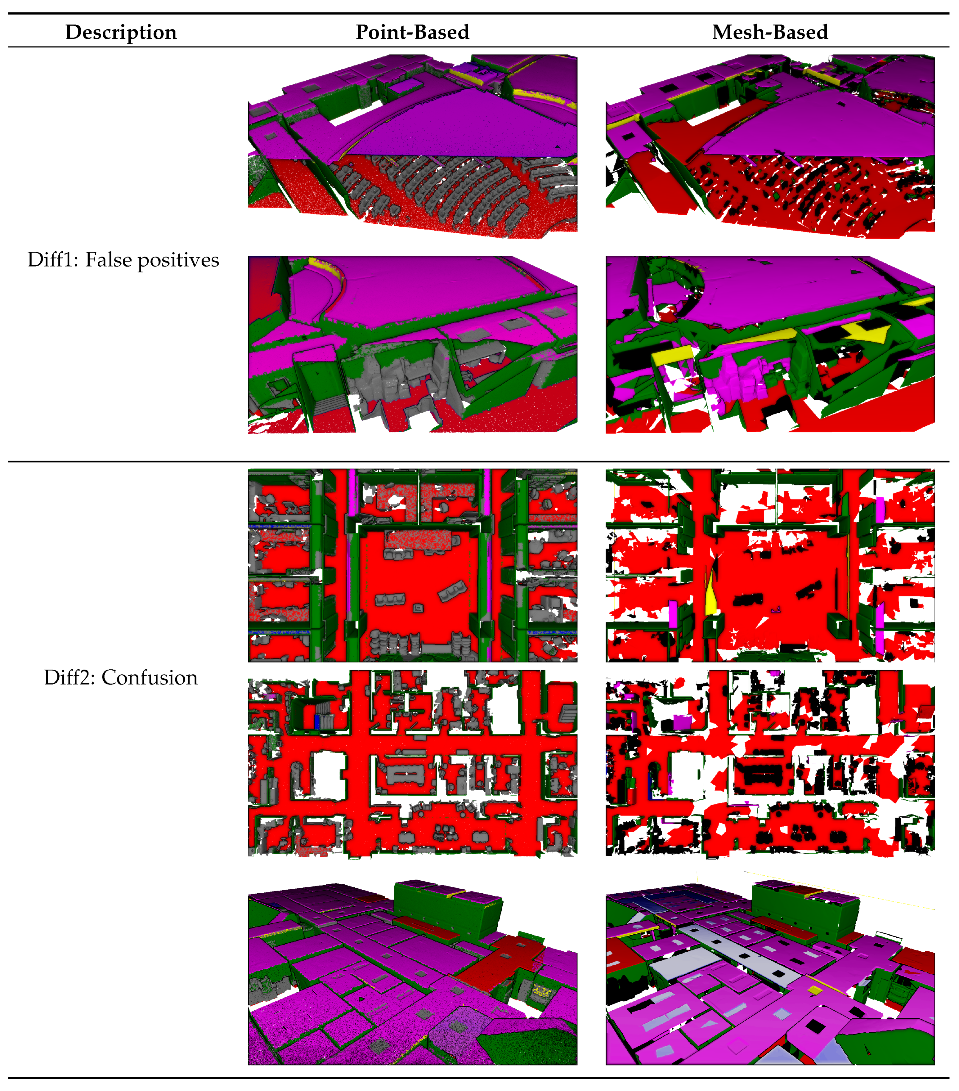
The visual inspection is conducted on the final classification of both datasets. First, both geometries are metrically compared to each other. The Euclidean distance is determined between both datasets and the deviation metrics are evaluated. Next, a visual study is conducted of the classification of both datasets. Several callouts are made of the different areas of the Stanford dataset and compared for both methods. The target of the visual inspection is to confirm the metrics of the classification tests and to evaluate false positives.
5. Results
The experiments are conducted on the Stanford 2D-3D-Semantics Dataset (2D-3D-S) [92]. It contains 6 large indoor spaces of 3 buildings on the Stanford campus. It was captured using the Matterport Gen1 RGB-D sensor resulting in a point cloud with 695,878,620 points linked to 6 meshes with a total of 648,698 faces. Each dataset is composed of the raw 3D point clouds, the extracted mesh geometry and the semantic labels. The mesh and point clouds serve as the main input to the interpretation pipeline while the semantic labels serve as the ground truth for the classification. Overall, the datasets pose a challenging test for classification procedures. The environments were captured under realistic conditions and contain significant clutter, occlusions and many different instances of each class. The point clouds were manually annotated per area by [92] with a wide variety of classes, which in this experiment are restructured into ceiling, floor, wall, beam and other (including all the furniture classes, the windows and the doors).
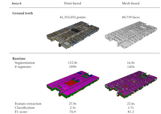
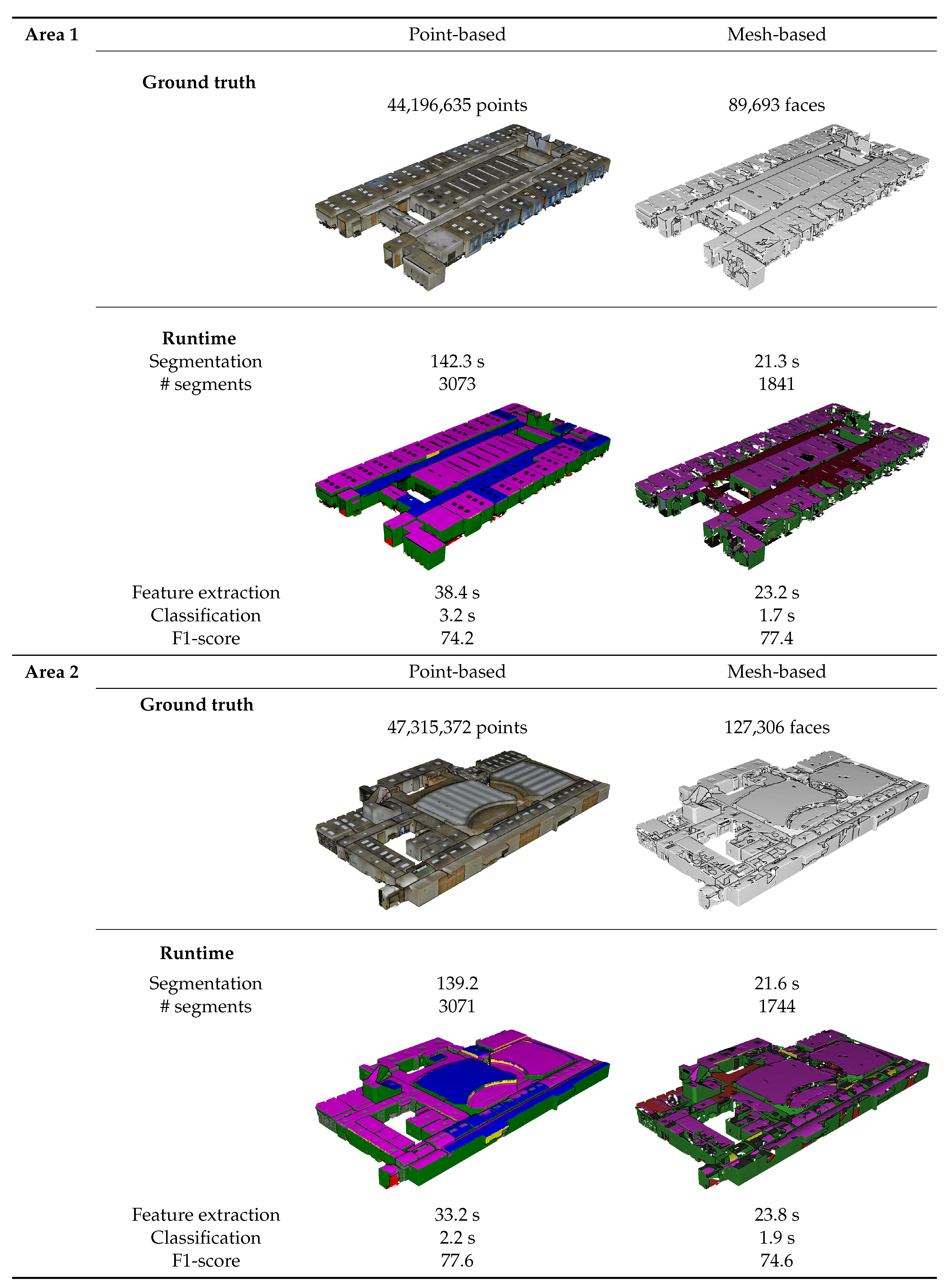
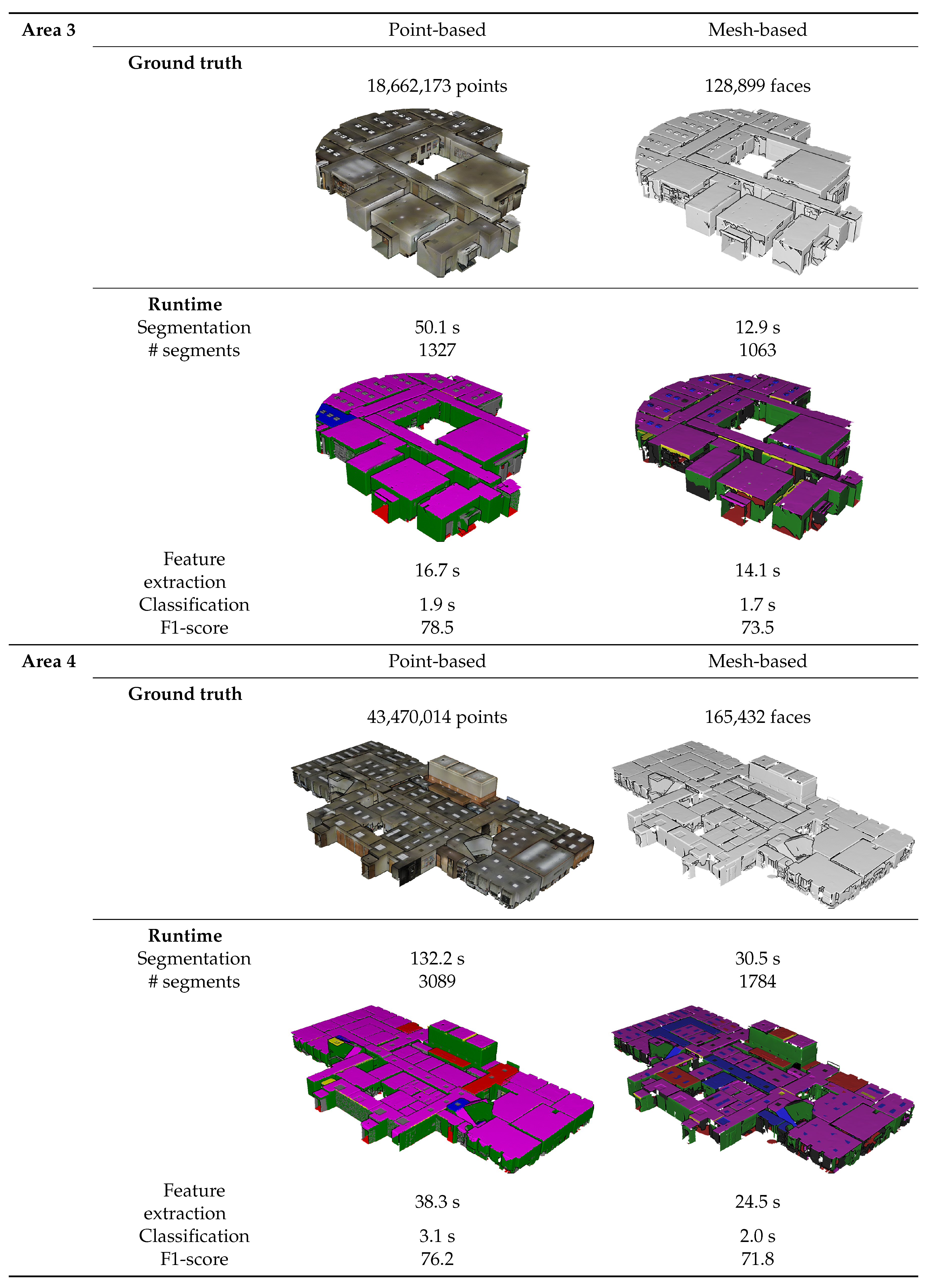
Prior to the tests, each dataset is segmented into smooth planar segments as shown in Table 5 and Figure 4, Figure 5 and Figure 6. Both datasets were segmented with similar parameters to achieve a proper segmentation of the building interiors. Table 5 depicts the number of segments that was created for each class. Overall, proper segments are extracted from both datasets. However, there are several differences between both procedures. First, the processing times of the point clouds are significantly higher than those of the meshes. This is expected since the meshing (of which the processing time is not included here) reduces the number of observations by over 90% compared to the initial point cloud. Second, the number of segments created from the point clouds are significantly higher than with the meshes due to the increased noise, observations and holes. Floors are an exception to this as these segments contain little curvature and detailing and are less obscured by other objects in comparison to other object types. These differences impact the processing time of the segmentation and the classification of the point clouds. However, this is counter-balanced by the fact that the point cloud does not necessitate any preprocessing step to transform it into a mesh, which is often a very time-consuming process. The resulting point-based and mesh-based segments S are the main input for the feature extraction, the classification and the visual inspection.
The results of the feature evaluation are listed in Table 6 and Table 7. It is observed that several features take on extreme values which is expected as the feature extraction is not normally distributed and focus on discriminativeness. The IQRs of both methods have little overlap between classes and the IQRs themselves have limited ranges for most classes. For instance, observations of walls and ceilings are systematically larger and have higher normal similarity than observations of clutter which is marked by randomness. When combined, these features are also useful to identify error prone segments such as doors, which have a distinct aspect ratio (height and width). Based on the boxplots, it is expected that both approaches will provide promising classification results. Despite their individual performance, there are significant differences between the feature values of both methods due to the differences between the point-based and the mesh-based segments. First, the median, IQR and skew of each class significantly deviate depending on the feature. Table 7 reports maximum feature score deviations of 0.17 for the median, 39% for the average skew and 0.19 for the IQR. As a result, there are differences in OVL of up to 0.23 between the classes and only 0.01 OVL between the methods as a whole. These differences are caused by the segment’s shape as well as by their context. For instance, the surface area feature reveals that mesh-based segments on average score 0.13 higher than their point-based counterparts indicating an increased size. This significantly affects the number of segments created (which is up to 2 times higher for the point clouds) which in turn impacts the IQR of each class. On average, the point-based segments generate 0.19 larger IQRs than the mesh-based segments, which can affect the classification. While these differences vary depending on the feature, Table 7 shows that there are systematic deviations between the segments of both methods. Overall, the IQRs of mesh-based segments are 0.07 smaller and have 0.08 less overlap, making them respectively more distinct and discriminative.
Table 8 shows the result of the classification and Table 4, Table 5 and Table 6 show the processing times. Each column in Table 8 depicts the F1 score for each method for the different classes. Overall, both methods were able to classify the segments generated on the in total 300 million points and 700,000 meshes. The average F1 score for the point-based and the mesh-based method are respectively 75.9% and 75.5%, which is promising considering the obstacles of the benchmark data and that the data was solely used for validation and not training. Both F1 scores are similar which indicates that the classification model was properly trained for the point-based segments despite the discrepancy in feature values. This can be attributed to the Bagged Trees capacity to deal with high variance datasets such as building environments. However, the F1 scores in Table 8 only provide the overall statistics of the classification, of which the clutter is a significant part. To make an in-depth comparison between both methods, a visual inspection is required.
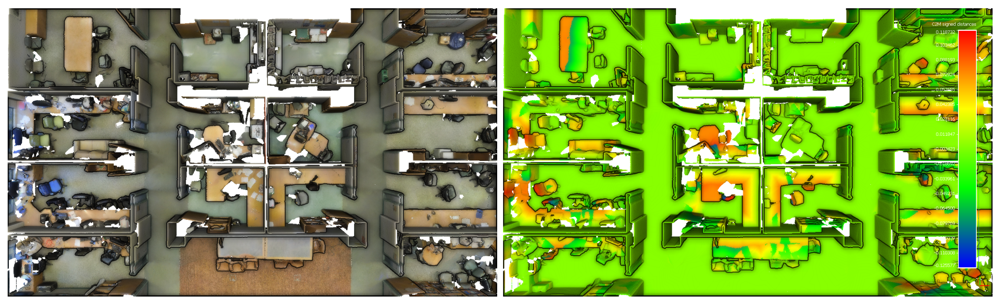
The results of the visual inspection are shown in Figure 7. The maximal deviation of the mesh geometry is 13 cm from the point cloud, but on average, the standard deviation is under 2.5 cm Figure 8. Concerning structural elements, this error is less than 1 cm, due to their planar shape. However, we note that the meshing is prone to providing incomplete geometries due to the partial uneven sampling of the point geometry, which results in less triangles but more reliability of the mesh surface. We can see that both methods perform well on the varying scenarios and challenges posed by the datasets. The first thing to note, is that the point cloud presents an overall higher consistency due to “complete” nature of the spatial representation. Its mesh counterpart, as highlighted in the previous section, is less complete, but the accuracy of the classification is not highly impacted. The second thing to note, is that both methods largely agree for the main parts (walls, ceilings, floors), and the differences are mainly noticeable for elements connected to structural classes such as the clutter, bookcases and tables as illustrated in Diff1 from Figure 7. We also note that some beam elements are identified in the mesh modality whereas it is classified as wall in the point cloud dataset. Finally, we note that independent objects with a clear distinctiveness from wall elements (e.g., chairs) are correctly handled in both datasets with very little visual difference between modalities.
6. Discussion
In this section, the pros and cons of the point-based and the mesh-based approach are discussed. First, we study the impact of the geometry on the feature extraction between the point-based and the mesh-based method. A first major difference to discuss is that the mesh-based segments have smoother geometries with less noise, less holes and thus is more consistently connected to other segments. As a result, mesh segments are typically larger with more distinct local and contextual information. The experiments clearly show that meshing can positively impacts the feature extraction and leads to more discriminative shape features. In contrast, the point-based segments better represent the raw information of the point cloud without interpolation. While these segments contain noise or are affected by occlusions, they are not prone to potential errors that plague meshing operations, and are better suited for unsupervised workflows with minimal serialized breaking points. Instances such as falsely connected segments, falsely closed holes, non-manifold mesh faces and oversimplification of the scene can have a negative impact on the feature extraction and the subsequent classification. It is argued that with each added step to the process, additional errors are injected thus working close to the point clouds is recommended in this case. However, if the meshing is performed appropriately, more distinct and discriminative features values can be extracted from the segments.
The second difference between both methods is the impact on the classification results. To this end, one should consider both the F1 scores of the classification and the visual inspection of the different areas in the 2D-3D-S dataset. The experiments reveal that both geometric modalities deliver over 75% F1-scores. However, the metrics are nuanced as there is a major difference between small and large segments. The visual inspection in Figure 7 shows that the classification of the larger segments in the scene is near-identical. Therefore, the difference in F1 scores is mainly due to smaller segments where noise, occlusions and differences in surface area have a much higher impact. As these segments only make up a small portion of the total surface area of the scene, their significance is very limited. However, there are some occurrences of larger segments that are misclassified. For instance, some doors that were identified in the mesh-based classification are labeled as walls in the point-based classification. These errors are critical as they lead to an excess of walls in the project. However, it is revealed that despite the mesh-based approach properly identifying more of these occurrences, it still produces some of the same false positives as the point-based segment approach. For instance, the built-in closet in Figure 7 is misclassified by both methods due to its geometric similarity to a wall. This showcases the limitations of geometry-based classification tasks which are complementary to computer vision classification.
In summary, both methods are very capable of properly interpreting the majority of building environments through the proposed feature set. While meshing does improve the feature extraction and classification performance, one should consider the gain of adding such a preprocessing layer (meshing operation) for offline processes (which mesh-based classification are stuck to). As classification score performance goes, no distinct recommendation is emitted, as both obtain good scores under 1% difference.
7. Conclusions
This paper presents an overview of the impact of geometry representations on the classification of building components. More specifically, a comparison is made between point clouds and meshes which are the two most common geometry inputs for classification procedures. The goal is to study the differences between the two geometry types with respect to the segmentation, feature extraction and the classification. It is hypothesized that the difference in noise, holes, size and the amount of data can impact these procedures and by extent the success rate of geometry interpretation tasks. Through this study, developers and researchers can now make an informed decision about which geometry type to choose during classification procedures to achieve the desired result. This study is focused on the structural components of a building i.e., the floors, ceilings, walls and beams as these form the core of any structure and are the target of numerous classification procedures.
The following conclusions are derived from the experiments on the Stanford 2D-3D-Semantics Dataset (2D-3D-S). In terms of feature extraction, the experiments show improved feature discriminativeness and distinctness for the mesh-based features due to the reduced amounts of noise and holes compared to point clouds. On average, mesh-based segments are larger, have fewer overlapping features and have a lower dispersion than their point cloud counterparts. However, the impact on the overall classification itself is minimal based on the observed F1 scores. Overall, both methods have promising results (75.9% for point clouds and 75.5% for meshes) despite the clutter in the scenes. This shows that machine learning models such as Bagged Trees are robust against high variance datasets that are building environments. The final experiment is a visual inspection, which revealed that both methods can deal with typical false positives such as doors and closets. Overall, it is concluded that the preprocessing of point clouds to mesh geometry leads to more distinct and discriminative features but not necessarily to a better classification. However, the significant data reduction which is achieved during the meshing allows for more complex features to be computed from the segments while maintaining performance. In procedures which cannot afford this preprocessing or to limit the serialization of potential break points in unsupervised workflows, methods using point cloud segments also offer promising classification results.
In terms of future work, there are several research topics that can be further investigated. For instance, an interesting field of research is the switch from human driven features to machine generated features much like the ones used in computer vision. Significant work also must be done to extend the generalization of building classification to make the method more robust to the variety of objects in the scene. The retrieval of windows and doors is also considered to be the next step in the classification procedure, which can use the structure information as prior knowledge.
Author Contributions
M.B., F.P. and M.V. contributed equally to the work. All authors have read and agreed to the published version of the manuscript.
Funding
This project has received funding from the European Research Council (ERC) under the European Union’s Horizon 2020 research and innovation programme (grant agreement 779962), the VLAIO COOCK programme (grant agreement HBC.2019.2509) and the Geomatics research group of the Department of Civil Engineering, TC Construction at the KU Leuven in Belgium.
Conflicts of Interest
There are no conflicts of interest to report.
References
- Patraucean, V.; Armeni, I.; Nahangi, M.; Yeung, J.; Brilakis, I.; Haas, C. State of research in automatic as-built modelling. Adv. Eng. Inform. 2015, 29, 162–171. [Google Scholar] [CrossRef] [Green Version]
- Shirowzhan, S.; Sepasgozar, S.M.; Li, H.; Trinder, J.; Tang, P. Comparative analysis of machine learning and point-based algorithms for detecting 3D changes in buildings over time using bi-temporal lidar data. Autom. Constr. 2019, 105. [Google Scholar] [CrossRef]
- Volk, R.; Stengel, J.; Schultmann, F. Building Information Modeling (BIM) for existing buildings—Literature review and future needs. Autom. Constr. 2014, 38, 109–127. [Google Scholar] [CrossRef] [Green Version]
- Xiong, X.; Adan, A.; Akinci, B.; Huber, D. Automatic creation of semantically rich 3D building models from laser scanner data. Autom. Constr. 2013, 31, 325–337. [Google Scholar] [CrossRef] [Green Version]
- Nikoohemat, S.; Diakité, A.A.; Zlatanova, S.; Vosselman, G. Indoor 3D reconstruction from point clouds for optimal routing in complex buildings to support disaster management. Autom. Constr. 2020, 113, 103109. [Google Scholar] [CrossRef]
- Poux, F.; Billen, R. A Smart Point Cloud Infrastructure for intelligent environments. Laser Scanning 2019, 127–149. [Google Scholar] [CrossRef]
- Lin, C.H.H.; Chen, J.Y.Y.; Su, P.L.L.; Chen, C.H.H. Eigen-feature analysis of weighted covariance matrices for LiDAR point cloud classification. ISPRS J. Photogramm. Remote Sens. 2014, 94, 70–79. [Google Scholar] [CrossRef]
- Bassier, M.; Van Genechten, B.; Vergauwen, M. Classification of sensor independent point cloud data of building objects using random forests. J. Build. Eng. 2019, 21, 468–477. [Google Scholar] [CrossRef]
- Boltcheva, D.; Lévy, B. Surface reconstruction by computing restricted Voronoi cells in parallel. CAD Comput. Aided Des. 2017, 90, 123–134. [Google Scholar] [CrossRef] [Green Version]
- Rouhani, M.; Lafarge, F.; Alliez, P. Semantic segmentation of 3D textured meshes for urban scene analysis. ISPRS J. Photogramm. Remote Sens. 2017, 123. [Google Scholar] [CrossRef] [Green Version]
- Dong, W.; Lan, J.; Liang, S.; Yao, W.; Zhan, Z. Selection of LiDAR geometric features with adaptive neighborhood size for urban land cover classification. Int. J. Appl. Earth Obs. Geoinf. 2017, 2017. [Google Scholar] [CrossRef]
- Weinmann, M.; Jutzi, B.; Hinz, S.; Mallet, C. Semantic point cloud interpretation based on optimal neighborhoods, relevant features and efficient classifiers. ISPRS J. Photogramm. Remote Sens. 2015, 105, 286–304. [Google Scholar] [CrossRef]
- Garstka, J.; Peters, G. Evaluation of Local 3-D Point Cloud Descriptors in Terms of Suitability for Object Classification. In Proceedings of the 13th International Conference on Informatics in Control, Automation and Robotics, Lisbon, Portugal, 29–31 July 2016; Volume 2, pp. 540–547. [Google Scholar]
- Poux, F.; Billen, R. Voxel-based 3D Point Cloud Semantic Segmentation: Unsupervised geometric and relationship featuring vs deep learning methods. ISPRS Int. J. Geo-Inf. 2019, 8, 213. [Google Scholar] [CrossRef] [Green Version]
- Bassier, M.; Ralf, K.; Van Genechten, B.; Vergauwen, M. Ifc Wall Reconstruction From Unstructured Point Clouds. ISPRS Ann. Photogramm. Remote Sens. Spat. Inf. Sci. 2018, IV, 4–7. [Google Scholar]
- Yue, H.; Chen, W.; Wu, X.; Liu, J. Fast 3D modeling in complex environments using a single Kinect sensor. Opt. Lasers Eng. 2014, 53, 104–111. [Google Scholar] [CrossRef]
- Lehtola, V.V.; Kaartinen, H.; Nüchter, A.; Kaijaluoto, R.; Kukko, A.; Litkey, P.; Honkavaara, E.; Rosnell, T.; Vaaja, M.T.; Virtanen, J.P.; et al. Comparison of the selected state-of-the-art 3D indoor scanning and point cloud generation methods. Remote Sens. 2017, 9, 796. [Google Scholar] [CrossRef] [Green Version]
- Quintana, B.; Prieto, S.A.; Adán, A.; Bosché, F. Door detection in 3D coloured point clouds of indoor environments. Autom. Constr. 2018, 85, 146–166. [Google Scholar] [CrossRef]
- Wolf, D.; Prankl, J.; Vincze, M. Fast Semantic Segmentation of 3D Point Clouds using a Dense CRF with Learned Parameters. In Proceedings of the IEEE International Conference on Robotics and Automation (ICRA) (2015), Seattle, WA, USA, 26–30 May 2015. [Google Scholar] [CrossRef]
- Nikoohemat, S.; Peter, M.; Oude Elberink, S.; Vosselman, G. Exploiting Indoor Mobile Laser Scanner Trajectories for Semantic Interpretation of Point Clouds. ISPRS Ann. Photogramm. Remote Sens. Spat. Inf. Sci. 2017, IV-2/W4, 355–362. [Google Scholar] [CrossRef] [Green Version]
- Poux, F.; Neuville, R.; Van Wersch, L.; Nys, G.A.; Billen, R. 3D Point Clouds in Archaeology: Advances in Acquisition, Processing and Knowledge Integration Applied to Quasi-Planar Objects. Geosciences 2017, 7, 96. [Google Scholar] [CrossRef] [Green Version]
- Bassier, M.; Bonduel, M.; Van Genechten, B.; Vergauwen, M. Segmentation of Large Unstructured Point Clouds using Octree-Based Region Growing and Conditional Random Fields. ISPRS—Int. Arch. Photogramm. Remote Sens. Spat. Inf. Sci. 2017, XLII-2/W8, 25–30. [Google Scholar] [CrossRef] [Green Version]
- Poux, F.; Neuville, R.; Hallot, P.; Billen, R. Model For Semantically Rich Point Cloud Data. ISPRS Ann. Photogramm. Remote Sens. Spat. Inf. Sci. 2017, 4, 107–115. [Google Scholar] [CrossRef] [Green Version]
- Han, S. Towards efficient implementation of an octree for a large 3D point cloud. Sensors 2018, 18, 4398. [Google Scholar] [CrossRef] [Green Version]
- Laine, S.; Karras, T. Efficient sparse voxel octrees. IEEE Trans. Vis. Comput. Graph. 2011, 17, 1048–1059. [Google Scholar] [CrossRef] [Green Version]
- Vo, A.V.; Truong-Hong, L.; Laefer, D.F.; Bertolotto, M. Octree-based region growing for point cloud segmentation. ISPRS J. Photogramm. Remote Sens. 2015, 104, 88–100. [Google Scholar] [CrossRef]
- Su, Y.T.; Bethel, J.; Hu, S. Octree-based segmentation for terrestrial LiDAR point cloud data in industrial applications. ISPRS J. Photogramm. Remote Sens. 2016, 113, 59–74. [Google Scholar] [CrossRef]
- Yang, B.; Dong, Z.; Zhao, G.; Dai, W. Hierarchical extraction of urban objects from mobile laser scanning data. ISPRS J. Photogramm. Remote Sens. 2015, 99, 45–57. [Google Scholar] [CrossRef]
- Wang, J.; Lindenbergh, R.; Menenti, M. SigVox—A 3D feature matching algorithm for automatic street object recognition in mobile laser scanning point clouds. ISPRS J. Photogramm. Remote Sens. 2017, 128. [Google Scholar] [CrossRef]
- Riggio, M.; Sandak, J.; Franke, S. Application of imaging techniques for detection of defects, damage and decay in timber structures on-site. Constr. Build. Mater. 2015, 101, 1241–1252. [Google Scholar] [CrossRef]
- Dimitrov, A.; Golparvar-Fard, M. Segmentation of building point cloud models including detailed architectural/structural features and MEP systems. Autom. Constr. 2015, 51, 32–45. [Google Scholar] [CrossRef]
- Boissonnat, J.D.; Ghosh, A. Manifold Reconstruction Using Tangential Delaunay Complexes. Discret. Comput. Geom. 2014, 51, 221–267. [Google Scholar] [CrossRef] [Green Version]
- Kazhdan, M.; Hoppe, H. Screened poisson surface reconstruction. ACM Trans. Graph. 2013, 32. [Google Scholar] [CrossRef] [Green Version]
- Berger, M.; Tagliasacchi, A.; Seversky, L.M.; Alliez, P.; Guennebaud, G.; Levine, J.A.; Sharf, A.; Silva, C.T. A Survey of Surface Reconstruction from Point Clouds. Comput. Graph. Forum 2017, 36. [Google Scholar] [CrossRef] [Green Version]
- Arikan, M.; Schwarzler, M.; Flory, S.; Maierhoffer, S. O-Snap: Optimization-Based Snapping for Modeling Architecture. arXiv 2013, arXiv:1204.6216v2. [Google Scholar] [CrossRef]
- Díaz-Vilariño, L.; Khoshelham, K.; Martínez-Sánchez, J.; Arias, P. 3D modeling of building indoor spaces and closed doors from imagery and point clouds. Sensors 2015, 15, 3491–3512. [Google Scholar] [CrossRef] [Green Version]
- Holz, D.; Behnke, S. Approximate triangulation and region growing for efficient segmentation and smoothing of range images. Robot. Auton. Syst. 2014, 62, 1282–1293. [Google Scholar] [CrossRef]
- Habib, A.; Lin, Y.J. Multi-class simultaneous adaptive segmentation and quality control of point cloud data. Remote Sens. 2016, 8, 104. [Google Scholar] [CrossRef] [Green Version]
- Nguyen, A.; Le, B. 3D point cloud segmentation: A survey. In Proceedings of the 2013 6th IEEE Conference, Manila, Philippines, 12–15 November 2013; pp. 225–230. [Google Scholar] [CrossRef]
- Xiang, B.; Yao, J.; Lu, X.; Li, L.; Xie, R.; Li, J. Segmentation-based classification for 3D point clouds in the road environment. Int. J. Remote Sens. 2018, 39. [Google Scholar] [CrossRef]
- Lin, Y.; Wang, C.; Cheng, J.; Chen, B.; Jia, F.; Chen, Z.; Li, J. Line segment extraction for large scale unorganized point clouds. ISPRS J. Photogramm. Remote Sens. 2015, 102, 172–183. [Google Scholar] [CrossRef]
- Fan, Y.; Wang, M.; Geng, N.; He, D.; Chang, J.; Zhang, J.J. A self-adaptive segmentation method for a point cloud. Vis. Comput. 2017. [Google Scholar] [CrossRef]
- Vosselman, G.; Rottensteiner, F. Contextual segment-based classification of airborne laser scanner data. ISPRS J. Photogramm. Remote Sens. 2017. [Google Scholar] [CrossRef]
- Grilli, E.; Menna, F.; Remondino, F.; Scanning, L.; Scanner, L. A review of point clouds segmentation and classification algorithms. Int. Arch. Photogramm. Remote Sens. Spat. Inf. 2017, XLII. [Google Scholar] [CrossRef] [Green Version]
- Weinmann, M.; Weinmann, M.; Mallet, C.; Brédif, M. A classification-segmentation framework for the detection of individual trees in dense MMS point cloud data acquired in urban areas. Remote Sens. 2017, 9, 3277. [Google Scholar] [CrossRef] [Green Version]
- Guinard, S.; Landrieu, L. Weakly supervised segmentation-aided classification of urban scenes from 3D LiDAR point clouds. ISPRS J. Photogramm. Remote Sens. 2017, I, 1–10. [Google Scholar] [CrossRef] [Green Version]
- Lin, Y.; Wang, C.; Zhai, D.; Li, W.; Li, J. Toward better boundary preserved supervoxel segmentation for 3D point clouds. ISPRS J. Photogramm. Remote Sens. 2018, 2018. [Google Scholar] [CrossRef]
- Nguyen, D.T.; Hua, B.S.; Yu, L.F.; Yeung, S.K. A Robust 3D-2D Interactive Tool for Scene Segmentation and Annotation. IEEE Trans. Vis. Comput. Graph. 2018, 24, 3005–3018. [Google Scholar] [CrossRef] [PubMed] [Green Version]
- Dong, Z.; Yang, B.; Hu, P.; Scherer, S. An efficient global energy optimization approach for robust 3D plane segmentation of point clouds. ISPRS J. Photogramm. Remote Sens. 2018, 137, 112–133. [Google Scholar] [CrossRef]
- Papon, J.; Kulvicius, T.; Aksoy, E.E.; Florentin, W. Point Cloud Video Object Segmentation using a Persistent Supervoxel. In Proceedings of the IEEE/RSJ International Conference on Intelligent Robots and Systems (IROS), Tokyo, Japan, 3–7 November 2013; pp. 3712–3718. [Google Scholar]
- Aijazi, A.K.; Checchin, P.; Trassoudaine, L. Super-voxel based segmentation and classification of 3D urban landscapes with evaluation and comparison. Springer Tracts Adv. Robot. 2014, 92, 511–526. [Google Scholar] [CrossRef]
- Walsh, S.B.; Borello, D.J.; Guldur, B.; Hajjar, J.F. Data processing of point clouds for object detection for structural engineering applications. Comput.-Aided Civ. Infrastruct. Eng. 2013, 28, 495–508. [Google Scholar] [CrossRef]
- Previtali, M.; Scaioni, M.; Barazzetti, L.; Brumana, R. A flexible methodology for outdoor/indoor building reconstruction from occluded point clouds. ISPRS Ann. Photogramm. Remote Sens. Spat. Inf. Sci. 2014, II-3, 119–126. [Google Scholar] [CrossRef] [Green Version]
- Ochmann, S.; Vock, R.; Klein, R. Automatic reconstruction of fully volumetric 3D building models from oriented point clouds. ISPRS J. Photogramm. Remote Sens. 2019, 151, 251–262. [Google Scholar] [CrossRef] [Green Version]
- Oesau, S.; Lafarge, F.; Alliez, P. Indoor scene reconstruction using feature sensitive primitive extraction and graph-cut. ISPRS J. Photogramm. Remote Sens. 2014, 90, 68–82. [Google Scholar] [CrossRef] [Green Version]
- Czerniawski, T.; Sankaran, B.; Nahangi, M.; Haas, C.; Leite, F. 6D DBSCAN-based segmentation of building point clouds for planar object classification. Autom. Constr. 2018, 88, 44–58. [Google Scholar] [CrossRef]
- Rashad, M.; Khamiss, M.; Mousa, M. A review on Mesh Segmentation Techniques. Int. J. Eng. Innov. Technol. 2017. [Google Scholar] [CrossRef]
- Blomley, R.; Weinmann, M.; Leitloff, J.; Jutzi, B. Shape distribution features for point cloud analysis: A geometric histogram approach on multiple scales. ISPRS Ann. Photogramm. Remote Sens. Spat. Inf. Sci. 2014, II-3, 9–16. [Google Scholar] [CrossRef] [Green Version]
- Guo, Y.; Bennamoun, M.; Sohel, F.; Lu, M.; Wan, J. 3D object recognition in cluttered scenes with local surface features: A survey. IEEE Trans. Pattern Anal. Mach. Intell. 2014, 36. [Google Scholar] [CrossRef]
- Wang, C.; Cho, Y.K.; Kim, C. Automatic BIM component extraction from point clouds of existing buildings for sustainability applications. Autom. Constr. 2015, 56. [Google Scholar] [CrossRef]
- Zhu, Q.; Li, Y.; Hu, H.; Wu, B. Robust point cloud classification based on multi-level semantic relationships for urban scenes. ISPRS J. Photogramm. Remote Sens. 2017, 129, 86–102. [Google Scholar] [CrossRef]
- Husain, F.; Dellen, B.; Torras, C. Recognizing Point Clouds using Conditional Random Fields. In Proceedings of the 2014 22nd International Conference on Pattern Recognition (ICPR), Stockholm, Sweden, 24–28 August 2014. [Google Scholar]
- Niemeyer, J.; Rottensteiner, F.; Soergel, U. Contional Random Fields for lidar point cloud classification in complex urban areas. ISPRS Ann. Photogramm. Remote Sens. Spat. Inf. Sci. 2012, I, 263–268. [Google Scholar] [CrossRef] [Green Version]
- Anand, A.; Koppula, H.S.; Joachims, T.; Saxena, A. Contextually Guided Semantic Labeling and Search for 3D Point Clouds. Int. J. Robot. Res. 2012, 32, 19–34. [Google Scholar] [CrossRef]
- Guo, R.; Hoiem, D. Labeling Complete Surfaces in Scene Understanding. Int. J. Comput. Vis. 2014, 172–187. [Google Scholar] [CrossRef]
- Hong, S.; Jung, J.; Kim, S.; Cho, H.; Lee, J.; Heo, J. Semi-automated approach to indoor mapping for 3D as-built building information modeling. Comput. Environ. Urban Syst. 2015, 51, 34–46. [Google Scholar] [CrossRef]
- Ochmann, S.; Vock, R.; Wessel, R.; Klein, R. Automatic reconstruction of parametric building models from indoor point clouds. Comput. Graph. 2016, 54, 94–103. [Google Scholar] [CrossRef] [Green Version]
- Cui, Y.; Li, Q.; Yang, B.; Xiao, W.; Chen, C.; Dong, Z. Automatic 3-D Reconstruction of Indoor Environment With Mobile Laser Scanning Point Clouds. IEEE J. Sel. Top. Appl. Earth Obs. Remote Sens. 2019, 12, 3117–3130. [Google Scholar] [CrossRef] [Green Version]
- Tombari, F.; Salti, S.; Di Stefano, L. Unique signatures of histograms for local surface description. Lect. Notes Comput. Sci. 2010, 6313, 356–369. [Google Scholar] [CrossRef] [Green Version]
- Khan, S.H.; Bennamoun, M.; Sohel, F.; Togneri, R. Geometry driven semantic labeling of indoor scenes. Lect. Notes Comput. Sci. 2014, 8689, 679–694. [Google Scholar] [CrossRef]
- Guo, Y.; Sohel, F.; Bennamoun, M.; Lu, M.; Wan, J. Rotational projection statistics for 3D local surface description and object recognition. Int. J. Comput. Vis. 2013, 105, 63–86. [Google Scholar] [CrossRef] [Green Version]
- Arbeiter, G.; Fuchs, S.; Bormann, R.; Fischer, J.; Verl, A. Evaluation of 3D feature descriptors for classification of surface geometries in point clouds. IEEE Int. Conf. Intell. Robot. Syst. 2012, 1644–1650. [Google Scholar] [CrossRef]
- Maturana, D.; Scherer, S. VoxNet: A 3D Convolutional Neural Network for Real-Time Object Recognition. IEEE/RSJ Int. Conf. Intell. Robot. Syst. (IROS) 2015, 922–928. [Google Scholar] [CrossRef]
- Lotte, R.; Haala, N.; Karpina, M.; Aragao, L.; Shimabukuro, Y. 3D Façade Labeling over Complex Scenarios: A Case Study Using Convolutional Neural Network and Structure-From-Motion. Remote Sens. 2018, 10, 1435. [Google Scholar] [CrossRef] [Green Version]
- Chen, L.C.; Papandreou, G.; Kokkinos, I.; Murphy, K.; Yuille, A.L. DeepLab: Semantic Image Segmentation with Deep Convolutional Nets, Atrous Convolution, and Fully Connected CRFs. IEEE Trans. Pattern Anal. Mach. Intell. 2018, 40, 834–848. [Google Scholar] [CrossRef]
- Niemeyer, J.; Rottensteiner, F.; Soergel, U.; Heipke, C. Contextual classification of point clouds using a two-stage CRF. ISPRS Arch. 2015, 141–148. [Google Scholar] [CrossRef] [Green Version]
- Zhang, H.; Wang, J.; Fang, T.; Quan, L. Joint segmentation of images and scanned point cloud in large-scale street scenes with low-annotation cost. IEEE Trans. Image Process. 2014, 23, 4763–4772. [Google Scholar] [CrossRef] [PubMed]
- Hackel, T.; Wegner, J.D.; Schindler, K. Joint Classification and Contour Extraction of Large 3D Point Clouds. ISPRS J. Photogramm. Remote Sens. 2017, I, 231–245. [Google Scholar] [CrossRef]
- Landrieu, L.; Mallet, C.; Weinmann, M. Comparison of belief propagation and graph-cut approaches for contextual classification of 3D lidar point cloud data. In Proceedings of the 2017 IEEE International Geoscience and Remote Sensing Symposium (IGARSS), Fort Worth, TX, USA, 23–28 July 2017. [Google Scholar] [CrossRef] [Green Version]
- Xiong, B.; Jancosek, M.; Oude Elberink, S.; Vosselman, G. Flexible building primitives for 3D building modeling. ISPRS J. Photogramm. Remote Sens. 2015, 101, 275–290. [Google Scholar] [CrossRef]
- Kang, Z.; Yang, J. A probabilistic graphical model for the classification of mobile LiDAR point clouds. ISPRS J. Photogramm. Remote Sens. 2018, 2018. [Google Scholar] [CrossRef]
- Chane, C.S.; Mansouri, A.; Marzani, F.S.; Boochs, F. Integration of 3D and multispectral data for cultural heritage applications: Survey and perspectives. Image Vis. Comput. 2013, 31, 91–102. [Google Scholar] [CrossRef] [Green Version]
- Yang, J.; Shi, Z.K.; Wu, Z.Y. Towards automatic generation of as-built BIM: 3D building facade modeling and material recognition from images. Int. J. Autom. Comput. 2016, 13, 338–349. [Google Scholar] [CrossRef]
- Ramiya, A.M.; Nidamanuri, R.R.; Krishnan, R. Object-oriented semantic labelling of spectral–spatial LiDAR point cloud for urban land cover classification and buildings detection. Geocarto Int. 2015, 6049. [Google Scholar] [CrossRef]
- Weinmann, M.; Urban, S.; Hinz, S.; Jutzi, B.; Mallet, C. Distinctive 2D and 3D features for automated large-scale scene analysis in urban areas. Comput. Graph. 2015, 49. [Google Scholar] [CrossRef]
- Dittrich, A.; Weinmann, M.; Hinz, S. Analytical and numerical investigations on the accuracy and robustness of geometric features extracted from 3D point cloud data. ISPRS J. Photogramm. Remote Sens. 2017, 126, 195–208. [Google Scholar] [CrossRef]
- Breiman, L.E.O. Bagging Predictors. Mach. Learn. 1996, 24, 123–140. [Google Scholar] [CrossRef] [Green Version]
- Poux, F.; Neuville, R.; Nys, G.A.; Billen, R. 3D point cloud semantic modelling: Integrated framework for indoor spaces and furniture. Remote Sens. 2018, 10, 1412. [Google Scholar] [CrossRef] [Green Version]
- Dahlke, D.; Linkiewicz, M. Comparison between two generic 3d building reconstruction approaches - Point cloud based vs. Image processing based. Int. Arch. Photogramm. Remote Sens. Spat. Inf. Sci.—ISPRS Arch. 2016, 41, 599–604. [Google Scholar] [CrossRef]
- Koppula, H.S.; Anand, A.; Joachims, T.; Saxena, A. Semantic Labeling of 3D Point Clouds for Indoor Scenes. Adv. Neural Inf. Process. Syst. 2011, 1–9. [Google Scholar]
- Gao, Z.; Yu, Z.; Pang, X. A compact shape descriptor for triangular surface meshes. CAD Comput. Aided Des. 2014, 53, 62–69. [Google Scholar] [CrossRef] [PubMed] [Green Version]
- Armeni, I.; Sax, S.; Zamir, A.R.; Savarese, S.; Sax, A.; Zamir, A.R.; Savarese, S. Joint 2D-3D-Semantic Data for Indoor Scene Understanding. arXiv 2017, arXiv:1702.01105. [Google Scholar]
- Bassier, M.M.B.; Van Genechten, B.M.V. Octree-Based Region Growing and Conditional Random Fields. In Proceedings of the 2017 5th International Workshop LowCost 3D—Sensors, Algorithms, Applications, Hamburg, Germany, 28–29 November 2017; Volume XLII, pp. 28–29. [Google Scholar] [CrossRef] [Green Version]
- Munoz, D.; Bagnell, J.A.; Hebert, M. Stacked Hierarchical Labeling. In Proceedings of the European Conference on Computer Vision (2010), Crete, Greece, 5–11 September 2010. [Google Scholar]
- Armeni, I.; Sener, O.; Zamir, A.R.; Jiang, H.; Brilakis, I.; Fischer, M.; Savarese, S. 3D Semantic Parsing of Large-Scale Indoor Spaces. In Proceedings of the IEEE International Conference on Computer Vision and Pattern Recognition, Las Vegas, NV, USA, 27–30 June 2016; Volume 2016, pp. 1–10. [Google Scholar] [CrossRef]
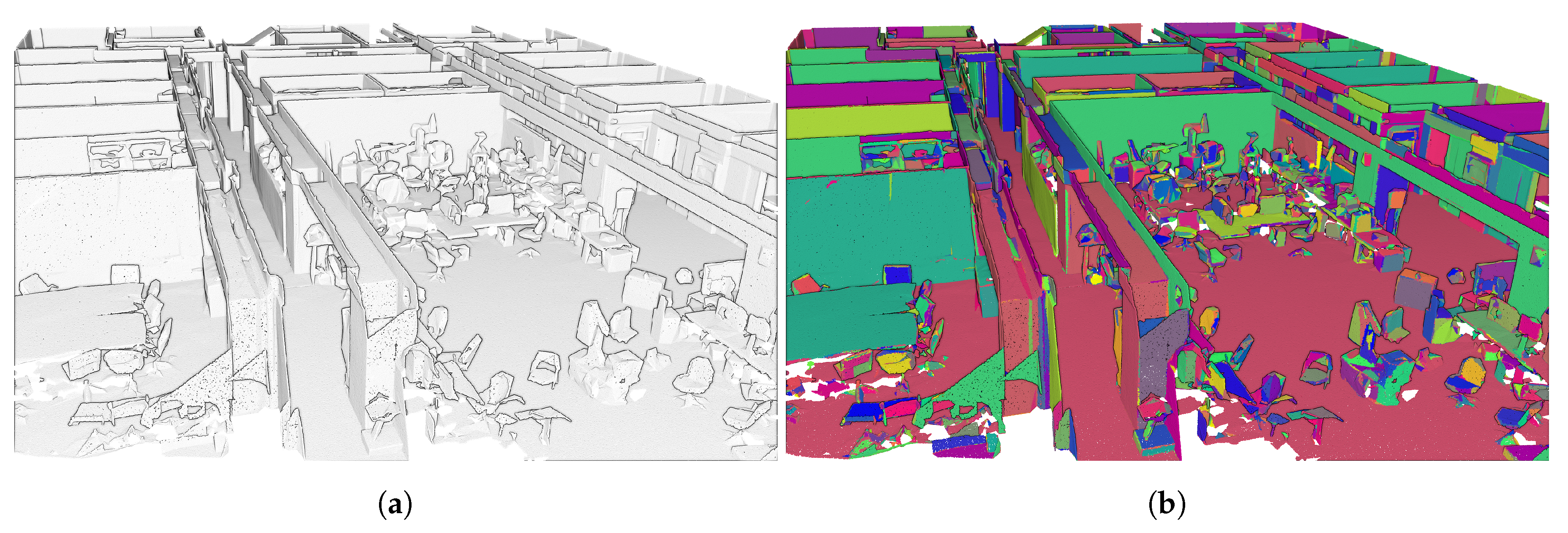
Figure 1.
Overview of the planar segments produced by the point cloud and meshing region growing. (a) Point cloud; (b) Segmentation.
Figure 1.
Overview of the planar segments produced by the point cloud and meshing region growing. (a) Point cloud; (b) Segmentation.

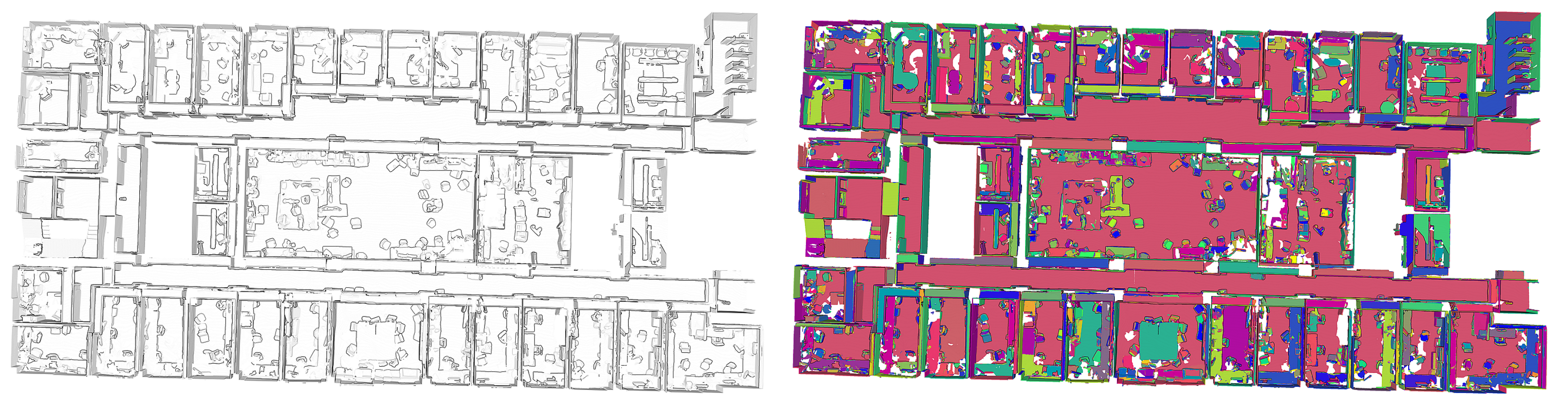
Figure 2.
Point Cloud Segmentation results on Area 1 of the Stanford 2D-3D-Semantics Dataset (2D-3D-S) [92].
Figure 2.
Point Cloud Segmentation results on Area 1 of the Stanford 2D-3D-Semantics Dataset (2D-3D-S) [92].

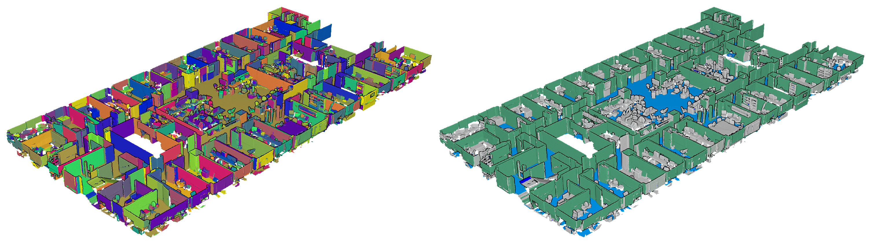
Figure 3.
From left to right: a segmented point cloud following [14]; The Classification results on segment-based features.
Figure 3.
From left to right: a segmented point cloud following [14]; The Classification results on segment-based features.

Figure 4.
Process information of the point-based and mesh-based procedures.

Figure 5.
Process information of the point-based and mesh-based procedures.

Figure 6.
Process information of the point-based and mesh-based procedures.

Figure 7.
Visual inspection of the classification differences between the point-based and the mesh-based segments approach: (top) False positives between clutter and structural classes and (bottom) confusion between structural classes.
Figure 7.
Visual inspection of the classification differences between the point-based and the mesh-based segments approach: (top) False positives between clutter and structural classes and (bottom) confusion between structural classes.

Figure 8.
Overview deviation analysis: (left) a point cloud extract of Area 6, (right) the singed Euclidean distance between both datasets ranging from −0.12 m in blue to 0.12 m in red.
Figure 8.
Overview deviation analysis: (left) a point cloud extract of Area 6, (right) the singed Euclidean distance between both datasets ranging from −0.12 m in blue to 0.12 m in red.


Table 1.
List of common 3D geometric shape features used for building interpretation.
| Eigenvector/Eigenvalues Features | Segment Features with Building Logic | ||
|---|---|---|---|
| change in curvature | z-component of the normal vector | ||
| linearity | xy-component of the normal vector | ||
| planarity | Dimensions | ||
| scatter or sphericity | Aspect ratio | ||
| omnivariance | Centre point Coordinates | ||
| anisotropy | Surface area | A | |
| eigenentropy | Density | ||
| sum of the eigenvalues |
Table 2.
Shape features extracted from each mesh/point cloud segment .
| Description | Definition Feature | Representation |
|---|---|---|
| Shape: Surface Area |  | |
| Shape: Orientation |  | |
| Shape: Width |  | |
| Shape: Height |  | |
| Shape: Normal similarity |  |
Table 3.
The proximity features extracted from each with respect to nearby reference segments R.
| Description | Definition Feature | Representation |
|---|---|---|
| Proximity: Coplanar distance to parallel segment |  | |
| Proximity: Distance to the nearest vertical segment |  | |
| Proximity: Vertical distance to the nearest horizontal segment above |  | |
| Proximity: Vertical distance to the nearest horizontal segment underneath |  | |
| Proximity: Average distance to n nearest large segments |  |
Table 4.
The topology features extracted from each with respect to a nearby reference segment r.
| Description | Definition Feature | Representation |
|---|---|---|
| Topology: Number of connected segments |  | |
| Topology: Unobstructed nearby segment in front or behind |  | |
| Topology: Presence of a large nearby segment above |  | |
| Topology: Presence of a large nearby segment below |  | |
| Topology: No presence of any segments above |  |
Table 5.
Object class statistics of the segments produced by the point- and mesh-based segmentation procedures. The top, middle and bottom row depict the number of segments that was generated per object class for respectively the ground truth, the point-based and the mesh-based approach. The right column shows the average number of segments created per object compared to the ground truth.
| Datasets | # Segments | |||||
|---|---|---|---|---|---|---|
| Ceiling | Floor | Wall | Beam | Other | Average | |
| Area 1 | 55 | 45 | 235 | 62 | 120 | 1 |
| 72 | 28 | 630 | 115 | 2228 | 5.9 | |
| 68 | 85 | 374 | 67 | 1247 | 3.6 | |
| Area 2 | 82 | 51 | 284 | 62 | 770 | 1 |
| 224 | 23 | 448 | 28 | 2348 | 2.4 | |
| 132 | 76 | 309 | 13 | 1214 | 1.4 | |
| Area 3 | 38 | 24 | 160 | 14 | 211 | 1 |
| 44 | 8 | 287 | 28 | 960 | 3.0 | |
| 37 | 30 | 278 | 26 | 692 | 2.4 | |
| Area 4 | 74 | 51 | 281 | 4 | 514 | 1 |
| 90 | 6 | 731 | 12 | 2250 | 3.3 | |
| 73 | 103 | 509 | 7 | 1092 | 1.9 | |
| Area 5 | 77 | 69 | 344 | 4 | 868 | 1 |
| 423 | 16 | 880 | 3 | 3224 | 3.3 | |
| 114 | 117 | 600 | 6 | 1029 | 1.4 | |
| Area 6 | 64 | 50 | 248 | 69 | 515 | 1 |
| 119 | 13 | 575 | 146 | 2154 | 3.2 | |
| 81 | 134 | 402 | 92 | 717 | 1.5 | |
Table 6.
Boxplot representation of the shape feature values produced by both methods for the different classes: (left) point-based classification and (right) the mesh-based classification.
Table 6.
Boxplot representation of the shape feature values produced by both methods for the different classes: (left) point-based classification and (right) the mesh-based classification.
| Shape Features | |
|---|---|
| Surface Area |  |
| Orientation |  |
| Width |  |
| Height |  |
| Normal similarity |  |
Table 7.
Table with the boxplot statistics of the feature extraction from the segments of the point-based and the mesh-based method. Notes: The difference between medians is a measure for data associativity, The average skew is a measure for the symmetry of the feature values, The average IQR per method is a measure for the data dispersion between both methods, the difference in OVL over all the classes for each method is a measure for difference in the feature discrimitiveness, the difference in OVL per class between both methods is a measure for the feature value similarity.
| Feature Comparison | Δ Median | Mean Skew | Δ IQR | OVL Class | OVL Methods | |
|---|---|---|---|---|---|---|
| Surface Area | m | 0.13 | 5 | −0.19 | 0.15 | 0.40 |
| p | −11 | 0.38 | ||||
| Orientation | m | −0.01 | −10 | −0.05 | 0.08 | 0.35 |
| p | 4 | 0.10 | ||||
| Width | m | 0.11 | 10 | −0.18 | 0.05 | 0.22 |
| p | −10 | 0.19 | ||||
| Height | m | 3 | −3 | −0.06 | 0.01 | 0.10 |
| p | −21 | 0.03 | ||||
| Normal similarity | m | −0.17 | 5 | 0.14 | 0.02 | 0.01 |
| p | 39 | 0.01 | ||||
| Average | m | 0.02 | 1.4 | −0.07 | 0.06 | 0.21 |
| p | 0.2 | 0.14 | ||||
Table 8.
F1-scores of the point-based (top row) and mesh-based (bottom row) classification of the 2D-3D-Semantics Dataset of Stanford [95].
Table 8.
F1-scores of the point-based (top row) and mesh-based (bottom row) classification of the 2D-3D-Semantics Dataset of Stanford [95].
| Datasets | F1-Scores | |||||
|---|---|---|---|---|---|---|
| Ceiling | Floor | Wall | Beam | Clutter | Average | |
| Area 1 | 72.5 | 75.7 | 81.0 | 39.1 | 77.8 | 74.2 |
| 95.0 | 69.6 | 74.3 | 39.4 | 81.1 | 77.4 | |
| Area 2 | 83.3 | 72.7 | 77.7 | 34.8 | 80.4 | 77.6 |
| 96.4 | 77.7 | 73.8 | 36.9 | 71.4 | 74.6 | |
| Area 3 | 88.5 | 77.2 | 77.5 | 36.6 | 77.3 | 78.5 |
| 77.9 | 71.4 | 63.3 | 39.4 | 75.6 | 73.5 | |
| Area 4 | 77.3 | 80.9 | 77.0 | 30.5 | 76.2 | 76.2 |
| 90.7 | 71.3 | 65.4 | 35.3 | 71.9 | 71.8 | |
| Area 5 | 70.1 | 50.8 | 77.4 | 29.3 | 71.4 | 71.8 |
| 76.7 | 47.2 | 71.4 | 31.2 | 76.2 | 74.5 | |
| Area 6 | 73.7 | 77.8 | 79.1 | 30.1 | 71.1 | 76.9 |
| 93.5 | 85.4 | 77.3 | 33.3 | 84.5 | 81.2 | |
© 2020 by the authors. Licensee MDPI, Basel, Switzerland. This article is an open access article distributed under the terms and conditions of the Creative Commons Attribution (CC BY) license (http://creativecommons.org/licenses/by/4.0/).
Share and Cite
MDPI and ACS Style
Bassier, M.; Vergauwen, M.; Poux, F. Point Cloud vs. Mesh Features for Building Interior Classification. Remote Sens. 2020, 12, 2224. https://0-doi-org.brum.beds.ac.uk/10.3390/rs12142224
AMA Style
Bassier M, Vergauwen M, Poux F. Point Cloud vs. Mesh Features for Building Interior Classification. Remote Sensing. 2020; 12(14):2224. https://0-doi-org.brum.beds.ac.uk/10.3390/rs12142224
Chicago/Turabian StyleBassier, Maarten, Maarten Vergauwen, and Florent Poux. 2020. "Point Cloud vs. Mesh Features for Building Interior Classification" Remote Sensing 12, no. 14: 2224. https://0-doi-org.brum.beds.ac.uk/10.3390/rs12142224
Note that from the first issue of 2016, this journal uses article numbers instead of page numbers. See further details here.