Using Unmanned Aerial Vehicles (UAV) for High-Resolution Reconstruction of Topography: The Structure from Motion Approach on Coastal Environments

Abstract
:1. Introduction
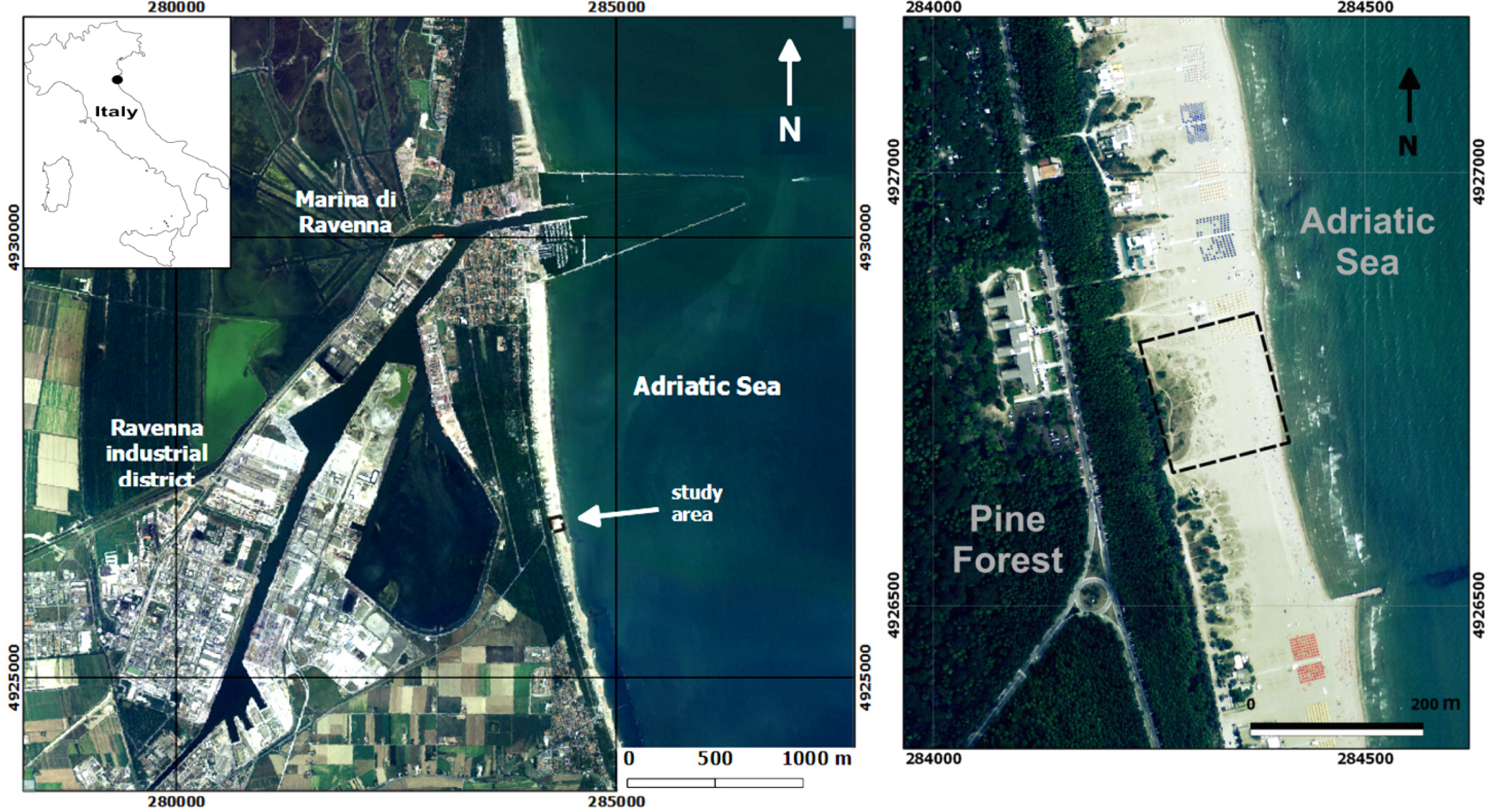
2. Study Area
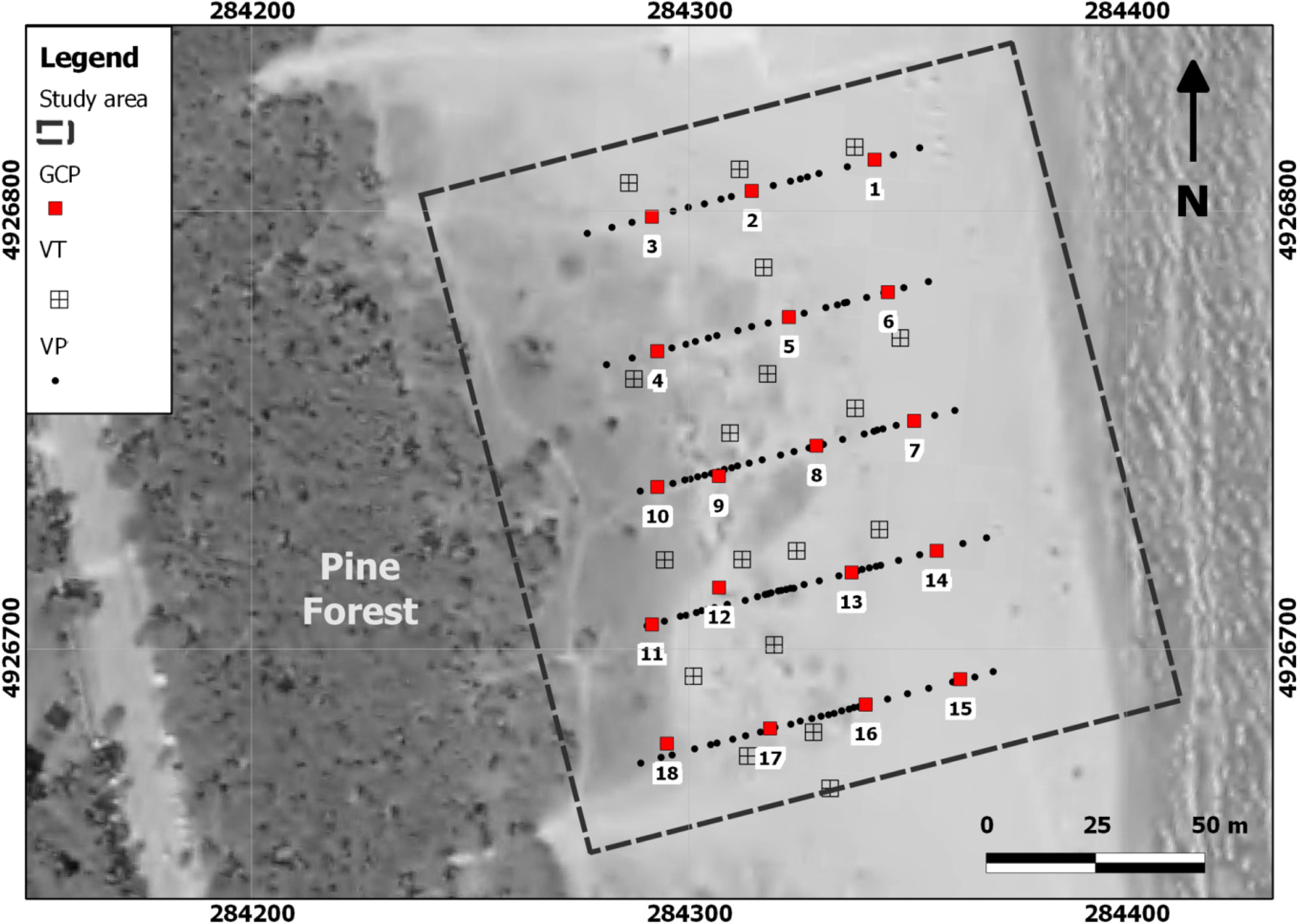
3. Methodology: GNSS, UAV, and TLS Surveys
3.2. The Unmanned Aerial Vehicle (UAV): Technical Specification and Survey
3.3. The Terrestrial Laser Scanner Survey
3.4. Software
4. Results
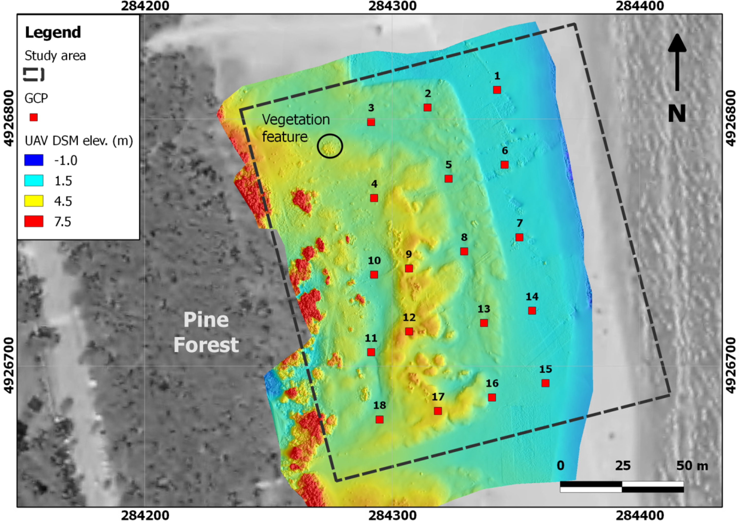
4.1. Point Cloud and DSM from UAV Images
4.2. Point Clouds and DSM from Terrestrial Laser Scanning (TLS) Survey
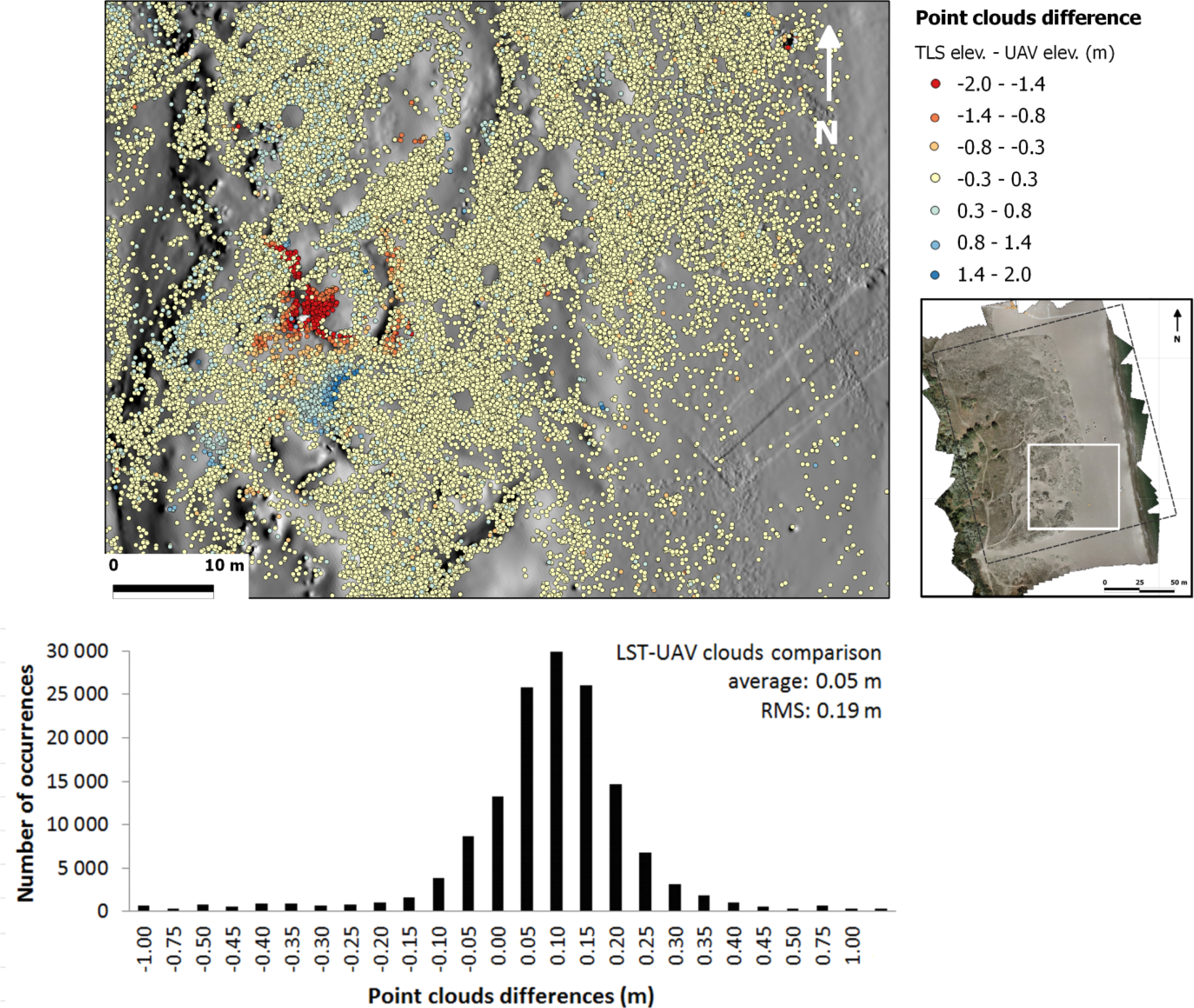
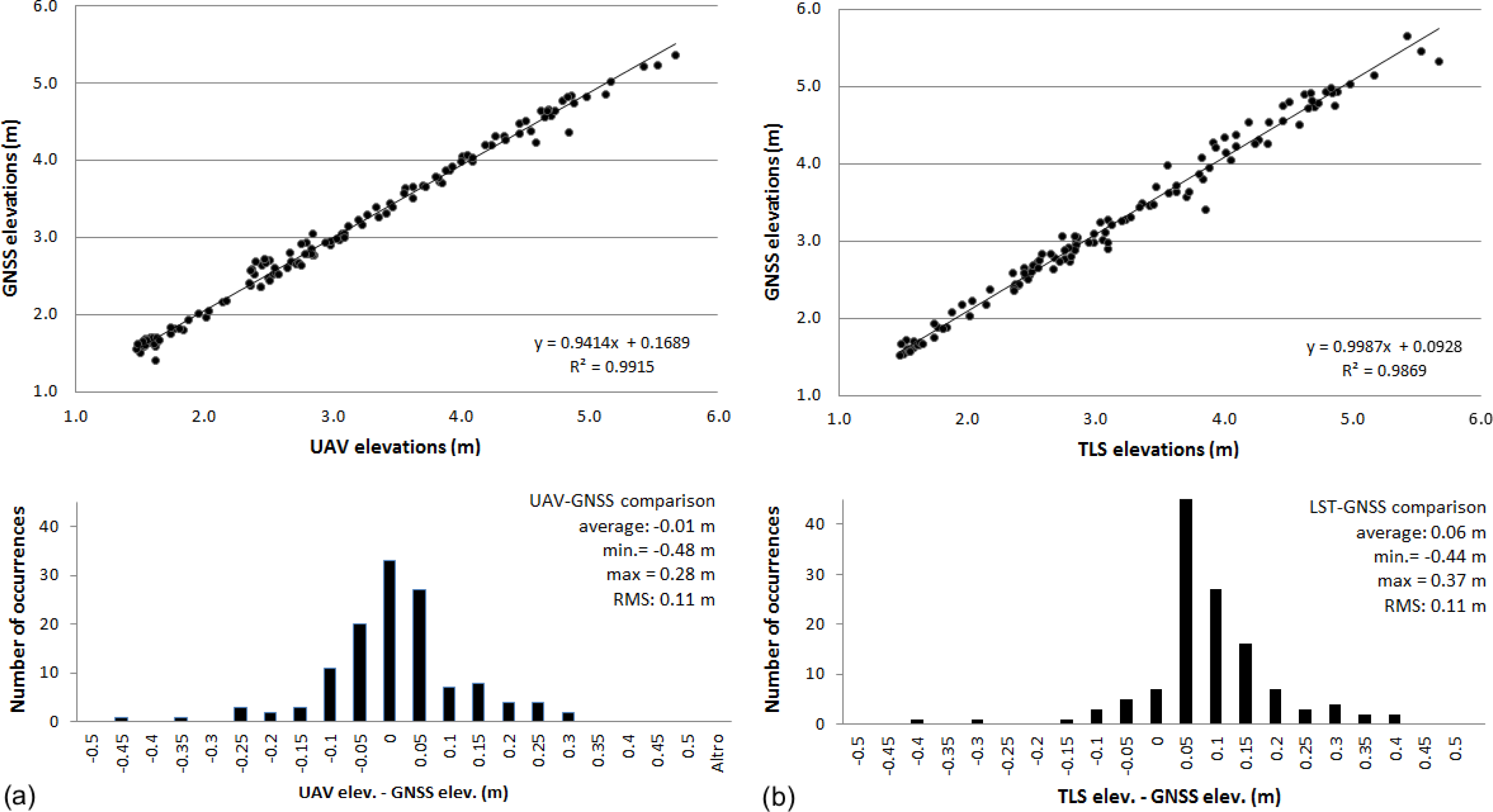
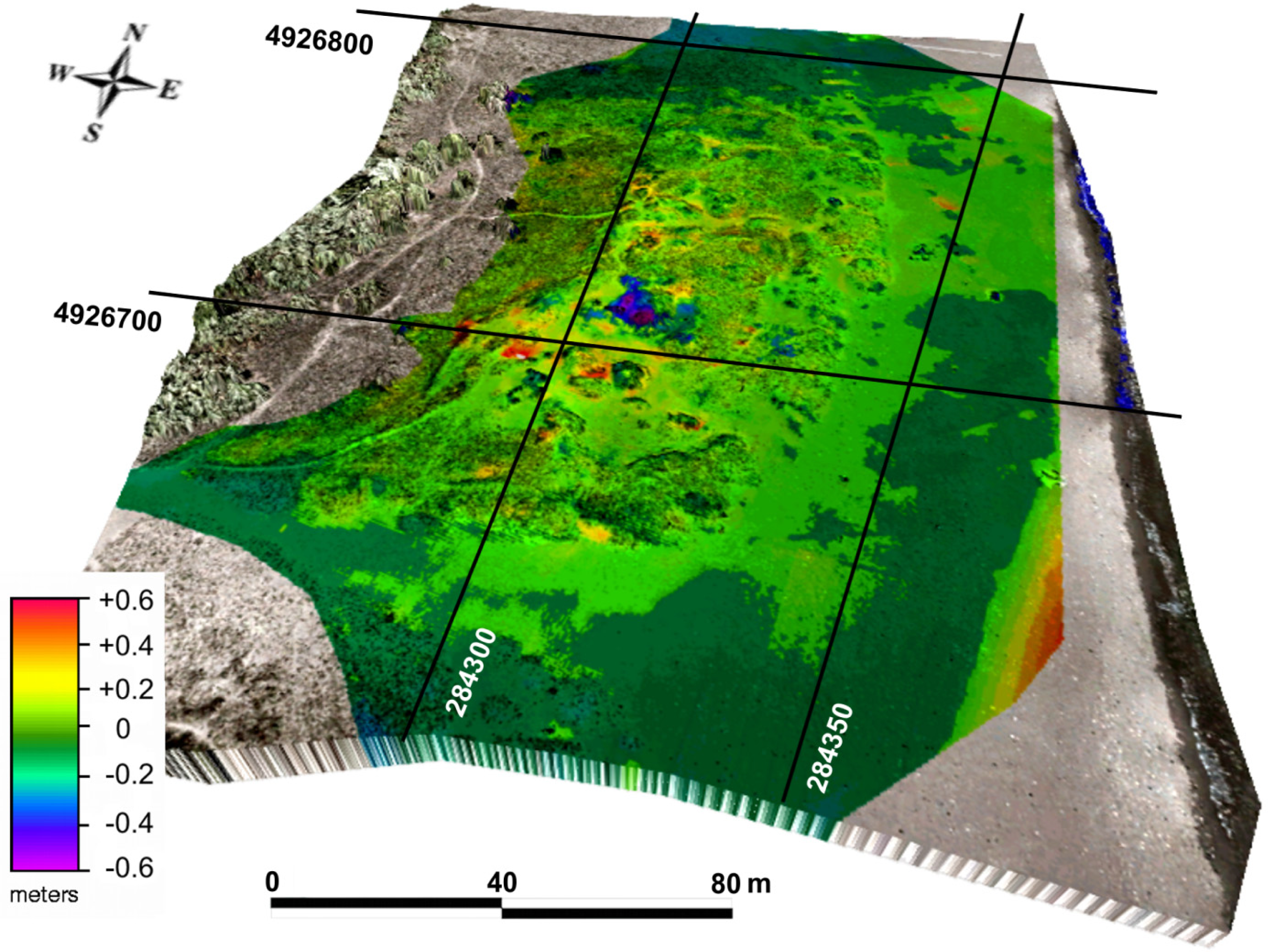
4.3. UAV, TLS, and GNSS Comparisons
5. Discussion
6. Conclusions
Conflicts of Interest
References
- Giambastiani, B.M.S.; Antonellini, M.; Gualbert, H.P.; Essink, O.; Stuurman, R.J. Saltwater intrusion in the unconfined coastal aquifer of Ravenna (Italy): A numerical model. J. Hydrol 2007, 340, 91–104. [Google Scholar]
- Chen, J.S.; Li, L.; Wang, J.Y.; Barry, D.A.; Sheng, X.F.; Gu, W.Z.; Zhao, X.; Chen, L. Water resources: Groundwater maintains dune landscape. Nature 2004, 432, 459–460. [Google Scholar]
- Brodu, N.; Lague, D. 3D Terrestrial lidar data classification of complex natural scenes using a multi-scale dimensionality criterion: Applications in geomorphology. ISPRS J. Photogramm. Remote Sens 2012, 68, 121–134. [Google Scholar]
- Nield, J.M.; Wiggs, G.F.S.; Squirrell, R.S. Aeolian sand strip mobility and protodune development on a drying beach: Examining surface moisture and surface roughness patterns measured by terrestrial laser scanning. Earth Surf. Process. Landf 2011, 4, 513–522. [Google Scholar]
- Nagihara, S.; Mulligan, K.R.; Xiong, W. Use of a three-dimensional laser scanner to digitally capture the topography of sand dunes in high spatial resolution. Earth Surf. Process. Landf 2004, 3, 391–398. [Google Scholar]
- Nelson, A.; Reuter, H.I.; Gessler, P. DEM Production Methods and Sources. In Geomorphometry Concepts, Software, Applications; Hengl, T., Reuter, H.I., Eds.; Elsevier: Amsterdam, The Netherlands, 2009; pp. 65–85. [Google Scholar]
- Houser, C.; Hapke, C.; Hamilton, S. Controls on coastal dune morphology, shoreline erosion and barrier island response to extreme storms. Geomorphology 2008, 3, 223–240. [Google Scholar]
- Sallenger, A.H.; Krabill, W.B.; Swift, R.N.; Brock, J.; List, J.; Hansen, M.; Holman, R.A.; Manizade, S.; Sontag, J.; Meredith, A.; et al. Evaluation of airborne topographic lidar for quantifying beach changes. J. Coastal Res 2003, 1, 125–133. [Google Scholar]
- Stockdonf, H.F.; Sallenger, A.H., Jr.; List, J.H.; Holman, R.A. Estimation of shoreline position and change using airborne topographic lidar data. J. Coast. Res 2002, 18, 502–513. [Google Scholar]
- Snavely, N; Seitz, S.M; Szeliski, R. Photo tourism: Exploring photo collections in 3D. ACM Trans. Graph 2006, 25, 835–846. [Google Scholar]
- Snavely, N. Scene Reconstruction and Visualization from Internet Photo Collections. Ph.D. Thesis, University of Washington, Seattle, WA, USA. 2008. [Google Scholar]
- Ullman, S. The interpretation of structure from motion. Proc. R. Soc. Lond. B 1979, 203, 405–426. [Google Scholar]
- Tomasi, C.; Kanade, T. Shape and motion from image streams under orthography: A factorization method. Int. J. Comput. Vis 1992, 9, 137–154. [Google Scholar]
- Poelman, C.J.; Kanade, T. A paraperspective factorization method for shape and motion recovery. IEEE. Trans. Pattern Anal. Mach. Intell 1997, 19, 97–108. [Google Scholar]
- Frahm, J-M.; Pollefeys, M.; Lazebnik, S.; Gallup, D.; Clipp, B.; Raguram, R.; Wu, C.; Zach, C.; Johnson, T. Fast robust large-scale mapping from video and internet photo collections. ISPRS J. Photogramm. Remote Sens 2010, 65, 538–549. [Google Scholar]
- Lingua, A.; Marenchino, D.; Nex, F. Performance analysis of the SIFT operator for automatic feature extraction and matching in photogrammetric applications. Sensors 2009, 9, 3745–3766. [Google Scholar]
- Barazzetti, L.; Remondino, F.; Scaioni, M.; Brumana, R. Fully Automatic UAV Image-Based Sensor Orientation. Proceedings of the 2010 Canadian Geomatics Conference and Symposium of Commission I, Calgary, AB, Canada, 15–18 June 2010.
- Baltsavias, E.; Gruen, A.; Zhang, L.; Waser, L.T. High-quality image matching and automated generation of 3D tree models. Int. J. Remote Sens 2008, 29, 1243–1259. [Google Scholar]
- Fonstad, M.A.; Dietrich, J.T.; Courville, B.C.; Jensen, J.L; Carbonneau, P.E. Topographic structure from motion: A new development in photogrammetric measurement. Earth Surf. Process. Landf 2013, 38, 421–430. [Google Scholar]
- Rango, A.; Laliberte, A.; Herrick, J.E.; Winters, C.; Havstad, K.; Steele, C.; Browning, D. Unmanned aerial vehicle-based remote sensing for rangeland assessment, monitoring, and management. J. Appl. Remote Sens 2009, 3, 033542. [Google Scholar]
- Verhoeven, G. Providing an archaeological bird’s eye view—An overall picture of ground-based means to execute low-altitude aerial photography (LAAP) in archaeology. Archaeol. Prospect 2009, 16, 233–249. [Google Scholar]
- Verhoeven, G.; Loenders, J.; Vermeulen, F.; Docter, R. Helikite aerial photography (HAP)—A versatile means of unmanned, radio-controlled, low-altitude aerial archaeology. Archaeol. Prospect 2009, 16, 125–138. [Google Scholar]
- Mathews, A.; Jensen, J. Visualizing and quantifying vineyard canopy LAI using an unmanned aerial vehicle (UAV) collected high density structure from motion point cloud. Remote Sens 2013, 5, 2164–2183. [Google Scholar]
- D’Oleire-Oltmanns, S.; Marzolff, I.; Peter, K.; Ries, J. Unmanned aerial vehicle (UAV) for monitoring soil erosion in Morocco. Remote Sens 2012, 4, 3390–3416. [Google Scholar]
- Wallace, L.; Lucieer, A.; Watson, C.; Turner, D. Development of a UAV-LiDAR system with application to forest inventory. Remote Sens 2012, 4, 1519–1543. [Google Scholar]
- Hunt, E.; Hively, W.; Fujikawa, S.; Linden, D.; Daughtry, C.; McCarty, G. Acquisition of NIR-Green-Blue digital photographs from unmanned aircraft for crop monitoring. Remote Sens 2010, 2, 290–305. [Google Scholar]
- Fonstad, M.A.; Marcus, W.A. High resolution, basin extent observations and implications for understanding river form and process. Earth Surf. Process. Landf 2010, 35, 680–698. [Google Scholar]
- Turner, D.; Lucieer, A.; Watson, C. An automated technique for generating georectified mosaics from ultra-high resolution unmanned aerial vehicle (UAV) imagery, based on structure from motion (SfM) point clouds. Remote Sens 2012, 4, 1392–1410. [Google Scholar]
- Harwin, S.; Lucieer, A. Assessing the accuracy of georeferenced point clouds produced via multi-view stereopsis from unmanned aerial vehicle (UAV) imagery. Remote Sens 2012, 4, 1573–1599. [Google Scholar]
- Rosnell, T.; Honkavaara, E. Point cloud generation from aerial image data acquired by a quadrocopter type micro unmanned aerial vehicle and a digital still camera. Sensors 2012, 12, 453–480. [Google Scholar]
- Bryson, M.; Johnson-Roberson, M.; Murphy, R.J.; Bongiorno, D. Kite aerial photography for low-cost, ultra-high spatial resolution multi-spectral mapping of intertidal landscapes. PloS One 2013, 8, e73550. [Google Scholar]
- Wheaton, J.M.; Brasington, J.; Darby, S.E.; Sear, D.A. Accounting for uncertainty in DEMs from repeat topographic surveys: Improved sediment budgets. Earth Surf. Process. Landf 2010, 35, 136–156. [Google Scholar]
- Teatini, P.; Ferronato, M.; Gambolati, G.; Bertoni, W.; Gonella, M. A century of land subsidence in Ravenna, Italy. Env. Geol 2005, 47, 831–846. [Google Scholar]
- Carbognin, L.; Tosi, L. Interaction between climate changes, eustacy and land subsidence in the North Adriatic Region, Italy. Mar. Ecol. Prog. Ser 2002, 23, 38–50. [Google Scholar]
- Agisoft PhotoScan. User Manual: Professional Edition; Version 0.9.1; AgiSoft LLC: Petersburg, Russia, 2013. [Google Scholar]
- Seitz, S.; Curless, B.; Diebel, J.; Scharstein, D.; Szeliski, R. A Comparison and Evaluation of Multi-View Stereo Reconstruction Algorithms. Proceedings of the 2006 IEEE Computer Society Conference on Computer Vision and Pattern, Washington, DC, USA, 17–22 June 2006; pp. 519–528.
- Szeliski, R. Computer Vision: Algorithms and Applications; Springer-Verlag: London, UK, 2010. [Google Scholar]
- Verhoeven, G. Taking computer vision aloft—Archaeological three–dimensional reconstructions from aerial photographs with PhotoScan. Archaeol. Prospect 2011, 18, 67–73. [Google Scholar]
- Montreuil, A.; Joanna, B.; Chandler, J. Detecting seasonal variations in embryo dune morphology using a terrestrial laser scanner. J. Coast. Res 2013, 65, 1313–1318. [Google Scholar]


| Manufacturer | S.A.L. Engineering, Modena, Italy |
|---|---|
| Type | Micro-drone Hexacopter |
| Engine Power | 6 Electric Brushless |
| Dimension and weight | 100 cm, 3.3 kg (total weight for all equipment is approximately 5 kg) |
| Flight mode | Dual, automatic based on waypoints or base on wireless control |
| Endurance | Standard 20 min (+5 min safety) |
| Flexible camera configurations | Digital gimbal, Canon EOS 550D (focal length 27 mm), res. 5184 × 3456 Bi-axial roll and pitch control |
| Ground Control Station | 8-channels, UHF modem, telemetry for real time flight control, and path tracking on video within 5 km |
| GCP | UTM Coord (m) | Individual Residuals after the Transformation (m) | |||||
|---|---|---|---|---|---|---|---|
| East | North | Elev. | East | North | Elev. | 3D | |
| 1 | 284342.420 | 4926811.730 | 1.900 | 0.005 | 0.000 | −0.023 | 0.024 |
| 3 | 284291.510 | 4926798.710 | 2.720 | 0.022 | 0.016 | 0.160 | 0.162 |
| 4 | 284292.740 | 4926768.000 | 3.760 | 0.001 | 0.002 | −0.004 | 0.005 |
| 5 | 284322.820 | 4926775.800 | 2.770 | −0.005 | 0.009 | −0.081 | 0.082 |
| 7 | 284351.450 | 4926752.100 | 2.020 | 0.001 | 0.007 | −0.010 | 0.012 |
| 10 | 284292.760 | 4926737.020 | 2.890 | −0.007 | 0.000 | −0.153 | 0.153 |
| 13 | 284337.150 | 4926717.480 | 3.130 | −0.004 | 0.000 | −0.020 | 0.020 |
| 14 | 284356.590 | 4926722.440 | 1.970 | 0.001 | −0.001 | 0.005 | 0.005 |
| 15 | 284361.990 | 4926693.110 | 2.020 | 0.000 | 0.002 | 0.058 | 0.058 |
| 18 | 284294.940 | 4926678.390 | 3.500 | −0.004 | −0.006 | −0.008 | 0.011 |
| RMS | 0.008 | 0.007 | 0.077 | 0.078 | |||
© 2013 by the authors; licensee MDPI, Basel, Switzerland This article is an open access article distributed under the terms and conditions of the Creative Commons Attribution license ( http://creativecommons.org/licenses/by/3.0/).
Share and Cite
Mancini, F.; Dubbini, M.; Gattelli, M.; Stecchi, F.; Fabbri, S.; Gabbianelli, G. Using Unmanned Aerial Vehicles (UAV) for High-Resolution Reconstruction of Topography: The Structure from Motion Approach on Coastal Environments. Remote Sens. 2013, 5, 6880-6898. https://0-doi-org.brum.beds.ac.uk/10.3390/rs5126880
Mancini F, Dubbini M, Gattelli M, Stecchi F, Fabbri S, Gabbianelli G. Using Unmanned Aerial Vehicles (UAV) for High-Resolution Reconstruction of Topography: The Structure from Motion Approach on Coastal Environments. Remote Sensing. 2013; 5(12):6880-6898. https://0-doi-org.brum.beds.ac.uk/10.3390/rs5126880
Chicago/Turabian StyleMancini, Francesco, Marco Dubbini, Mario Gattelli, Francesco Stecchi, Stefano Fabbri, and Giovanni Gabbianelli. 2013. "Using Unmanned Aerial Vehicles (UAV) for High-Resolution Reconstruction of Topography: The Structure from Motion Approach on Coastal Environments" Remote Sensing 5, no. 12: 6880-6898. https://0-doi-org.brum.beds.ac.uk/10.3390/rs5126880