Remote Sensing of Submerged Aquatic Vegetation in a Shallow Non-Turbid River Using an Unmanned Aerial Vehicle

Abstract

A passive method for remote sensing of the nuisance green algae Cladophora glomerata in rivers is presented using an unmanned aerial vehicle (UAV). Included are methods for UAV operation, lens distortion correction, image georeferencing, and spectral analysis to support algal cover mapping. Eighteen aerial photography missions were conducted over the summer of 2013 using an off-the-shelf UAV and three-band, wide-angle, red, green, and blue (RGB) digital camera sensor. Images were post-processed, mosaicked, and georeferenced so automated classification and mapping could be completed. An adaptive cosine estimator (ACE) and spectral angle mapper (SAM) algorithm were used to complete the algal identification. Digital analysis of optical imagery correctly identified filamentous algae and background coverage 90% and 92% of the time, and tau coefficients were 0.82 and 0.84 for ACE and SAM, respectively. Thereafter, algal cover was characterized for a one-kilometer channel segment during each of the 18 UAV flights. Percent cover ranged from <5% to >50%, and increased immediately after vernal freshet, peaked in midsummer, and declined in the fall. Results indicate that optical remote sensing with UAV holds promise for completing spatially precise, and multi-temporal measurements of algae or submerged aquatic vegetation in shallow rivers with low turbidity and good optical transmission.

1. Introduction

Submerged aquatic vegetation (SAV), including both rooted macrophytes and attached macroalgae, play an important role in aquatic ecosystems providing food and cover for a wide range of species [1]. In flowing water, they remove toxins from the water column and sediments [2], contribute to primary productivity and biogeochemical cycling of autochthonous resource pools [3,4], and improve water quality by filtering nutrients and polluted runoff [1]. Stems, leaves, or filaments of SAV provide structure in an otherwise amorphous water column, increasing diversity for vertebrates and invertebrates [4], and stabilizing streambeds [2]. SAV moreover are a barometer for water quality [1,5,6], integrating exposures of sunlight, nutrient, temperatures, and toxins to provide an overall understanding of ecosystem health. In this regard, ecological and water quality benefits of SAV are widespread.

However, certain types of SAV, primarily macroalgae, can become problematic due to cultural eutrophication (excess nitrogen and phosphorus from human activities). Shifts from desirable slow growing species to fast growing nuisance macroalgae can occur, which result in reduced biodiversity, declines in ecosystem health, or replacement of desired species [6,7]. In some instances, algal growth may reach nuisance levels that impair recreation, fish and aquatic life, and water quality beneficial uses. Upon these occasions, the relationship between algal cover, water quality, and other intrinsic properties such as benthic substrate, velocity, water depth, and nutrient and light availability must be understood to manage water resource systems appropriately and efficiently.

The filamentous algae Cladophora glomerata L. (Kuetzing) is one such nuisance algal species worldwide [8,9,10,11]. It grows attached to substrate in dense mats that disrupt benthic fauna and flora, foul lines and lures, or negatively affect both dissolved oxygen and pH in lakes [12,13] and rivers [10,14]. Upon sloughing, heavy growths may be aesthetically displeasing and interfere with foot travel near rivers and clog water intakes [13,15]. Widespread algal blooms also impact property values, tourism, and recreation (e.g., wading, swimming, and sport fishing) [16]. Consequently, mapping spatial algal cover, including Cladophora, is an important component of water-quality science and management that can be used to characterize the ecological well-being and aesthetic perception of a waterbody [17].

A number of remote sensing techniques have been developed to map the spatial cover of Cladophora. Past efforts have focused primarily on lakes [18,19,20], or coastal environments [21], and typically rely on aerial photography or multispectral satellite imaging to estimate benthic macroalgal cover. Hydroacoustic techniques have also been suggested [22,23], but are rarely used. For rivers, direct ocular observation is frequently employed [11,17], but this approach is site-specific, labor-intensive, and can characterize only a small percentage of a designated river reach. Alternatively, remote sensing (of rivers) has also been suggested, but is only exploratory [2,24,25]. As a consequence, further investigation of more robust and economical methods are needed to capture the spatial and temporal distribution of Cladophora in rivers for the purpose of mapping freshwater benthic algal cover.

The topic of optical remote sensing of rivers has received considerable attention due in part to the growing availability of lightweight digital or multispectral camera sensors and associated launch platforms [25,26]. Aquatic plants can be digitally identified with spectral reflectance [24,25,26,27], therefore SAV presumably can be characterized across multiple space and time scales with remotely sensed data [28]. Prior work (non-SAV related) has been completed using anything from handheld poles to commercial satellites [28], unmanned aerial vehicles (UAVs) [26], even kites and balloons [29,30] to map habitat, channel geomorphology, the water surface, or bathymetric features [2] at centimeter to meter scales. The use of conventional RGB aerial photography [25,26] or multispectral cameras [31] in these applications obviously requires the river water column to be clear and not obstructed by trees or overhanging banks [2,24].

A larger limitation of current remote sensing platforms for lotic investigation are cost, scale, or both. For example, widely available satellite products (e.g., Landsat, MODIS, or MERIS) have no up-front cost [20] and are useful for larger areas, but are too coarse to be of practical use in rivers since the typical resolution is >30 m. To the contrary, proprietary satellite imagery such as QuickBird, GeoEye-1 or Worldview-1 or -2, or commercial aerial photography (<0.5 m pixel area), provide sufficient resolution, but are prohibitively expensive for many applications [20,32]. As a consequence low-cost platforms are needed to map aquatic benthic environments in river settings.

Unmanned aerial vehicles (UAVs) are one possible solution to this problem [33,34,35,36,37,38]. Not only can UAVs obtain timely imagery over areas that are difficult or dangerous to access by traditional means [37], data can be acquired when the variable of interest needs to be measured, and usually at a lower cost, relative to other methods [39]. UAVs have been successfully applied for natural resource assessment, environmental monitoring, forest inventories, surveying, river corridor monitoring, plume tracking, wildlife management, avalanche patrols, and precision agriculture [33,34,35,37]; along with law enforcement, firefighting, border patrol, disaster relief, and search and rescue [40]. UAV use in mapping SAV for freshwater benthic ecology would also seem promising given widespread civilian and commercial use [33,35,41,42].

Accordingly, this article describes a consumer-friendly approach towards the use of UAV for remote sensing of freshwater benthic environments. It can be implemented with limited capital investment or specialized expertise. While the methods presented here are specific to monitoring the filamentous green algae Cladophora, many other potential applications of UAV and optical imaging exist in the field of aquatic ecology.

2. Materials and Methods

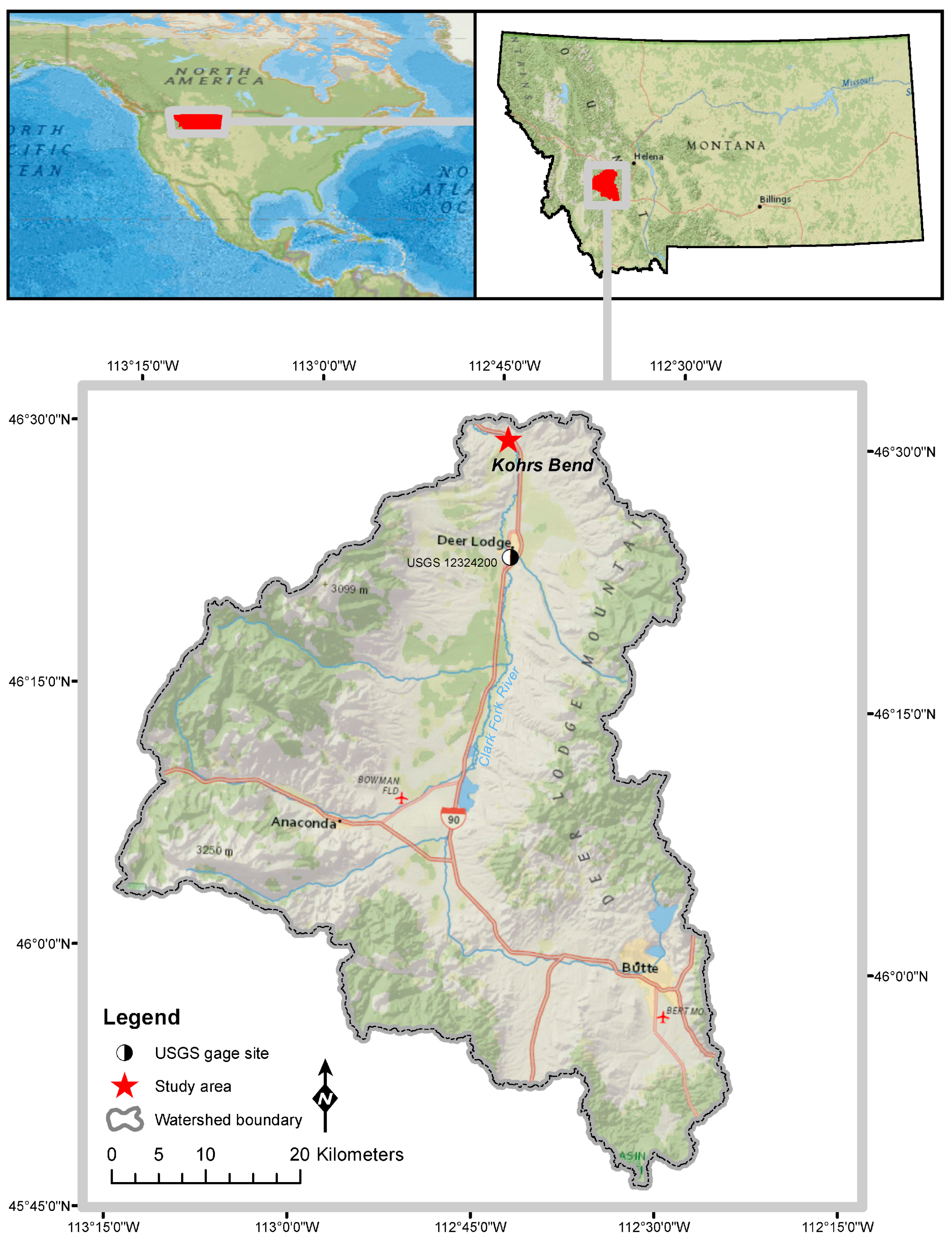
2.1. Study Area

UAV missions to map SAV were initiated on the Clark Fork River in western Montana during the summer of 2013 (Figure 1). The Clark Fork is a clear shallow 5th order Strahler [43] stream system with a long history of nuisance filamentous Cladophora growth [44,45,46]. In the spring, excessive bottom scour and turbidity remove much of the benthic biomass in the system, which is followed by a one to two month growing season when river conditions (e.g., temperature, velocity, and light) permit lush establishment of algal cover. Growth begins at the end of June, plateaus in August or September, and gradually recedes through October [44,45]. Studies were conducted at the Kohrs Fishing Access (FAS), which is a rural area located approximately 20 kilometers downstream of the city of Deer Lodge, MT (population 3120).

Figure 1. Vicinity and site map showing the Clark Fork River in western Montana and the Kohrs Bend study area.

Figure 1. Vicinity and site map showing the Clark Fork River in western Montana and the Kohrs Bend study area.

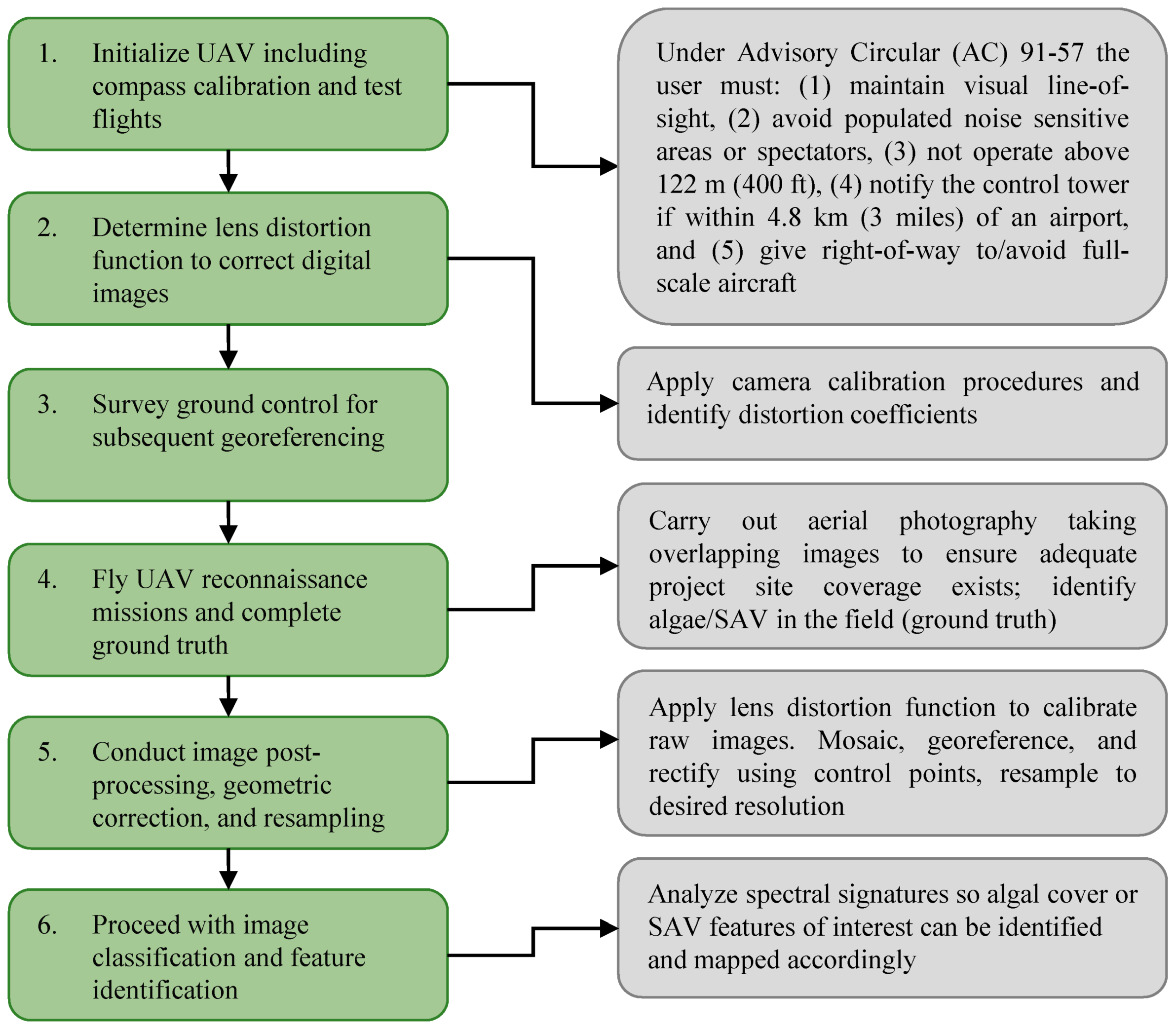
2.2. General Approach

Our approach to UAV optical imaging and mapping of river benthic algae is outlined in Figure 2. Of chief importance is to first test fly the UAV system prior to use away from spectators so that sensitive components such as the flight controls and imaging system can be evaluated. Thereafter, site preparatory work including setting ground control, scheduling flights, and characterizing the camera lens distortion function should be completed so that images can be post-processed to a rectilinear projection. Following these activities, data collection missions, image calibration, georeferencing, and spectral analysis can be completed to facilitate mapping.

Figure 2. Steps for unmanned aerial vehicle (UAV) use and subsequent algal cover mapping in shallow rivers.

Figure 2. Steps for unmanned aerial vehicle (UAV) use and subsequent algal cover mapping in shallow rivers.

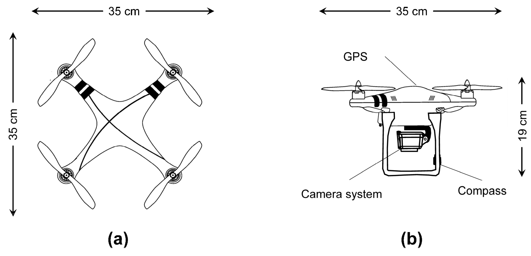
2.3. UAV Description

We used an inexpensive (<US$700) ready-to-fly unmanned multi-rotor aircraft manufactured by DJI industries with vertical takeoff and landing capability (VTOL). Dimensions of the UAV are 35 cm × 35 cm × 19 cm with a takeoff weight of <1000 g and payload of 200 g (Figure 3). Thus, only a small camera or imaging system can be affixed to it. The aircraft is equipped with a Naza-M Global Positioning System (GPS) autopilot that includes a position hold command with hovering accuracy of ±0.8 m vertically (±2.5 m horizontally) and a lost link failsafe function that activates if communication between the controller and the transmitter is lost (whereupon the system automatically returns to its takeoff location to land). Setup time for the UAV including prop balancing, instructional training, and compass calibration was <3 h. Thereafter the system was ready to fly within 10 min, had a communication distance of 300 m (6 channel 2.4GHz ISM), and could achieve a flight time of 10–15 min per battery pack (lithium-ion polymer).

2.4. Image Sensor

The camera used in this work was an inexpensive three-band GoPro Hero 3 (black) lightweight digital camera (Figure 3) with a 12MP sensor having a 129° (horizontal) field of view and image size of 3000 pixels × 4000 pixels (US$399). The GoPro sensor receives irradiance in the visible region (red, green, blue spectral bands) and stores it as a digital number from 0 to 255 in JPEG format. The system has a number of features that make it well suited for UAV studies. First, it has a Bluetooth wireless connection so the field of view and shutter can be monitored and activated remotely in real time via an iPhone app. It also has an intervalometer (time lapse) feature that is a good alternative to the wireless control. Finally, the camera has a waterproof case, which allows it to be used for underwater applications (i.e., ground truth of submerged aquatic vegetation). Hence, we were able to employ it interchangeably for both aerial photography and underwater ground truth imaging.

Figure 3. Unmanned aerial vehicle used in this study. (a) Top view showing propellers and motors; (b) Side view showing camera system, compass, and global positioning system (GPS). Drawings modified from the manufacturer. Accordingly, the aircraft would be classified as a small, low altitude short endurance UAV since it can be transported in a backpack carrying case, operates at very low altitudes (<330 m), and has short flight times (5–30 min) [35].

Figure 3. Unmanned aerial vehicle used in this study. (a) Top view showing propellers and motors; (b) Side view showing camera system, compass, and global positioning system (GPS). Drawings modified from the manufacturer. Accordingly, the aircraft would be classified as a small, low altitude short endurance UAV since it can be transported in a backpack carrying case, operates at very low altitudes (<330 m), and has short flight times (5–30 min) [35].

It should be noted in review of the camera described above, that consumer-grade digital cameras have been increasingly used by researchers for a variety of remote sensing applications due to their small size/weight and potential to store hundreds of images on a single flight [47]. However, wide-angle or fish-eye lenses are often needed to overcome the height and stability limitations of small UAV [41]. As a consequence, the GoPro wide-angle sensor provides information over a larger spatial area, with the drawback of added distortion on the edge of the image. Software subsequently can be used to remove distortion and correct the image back to a rectilinear lens projection [41]. The camera was mounted in a vertical position under the UAV; the only modification being drilling two small holes in a plastic mount to match the UAV thread pattern.

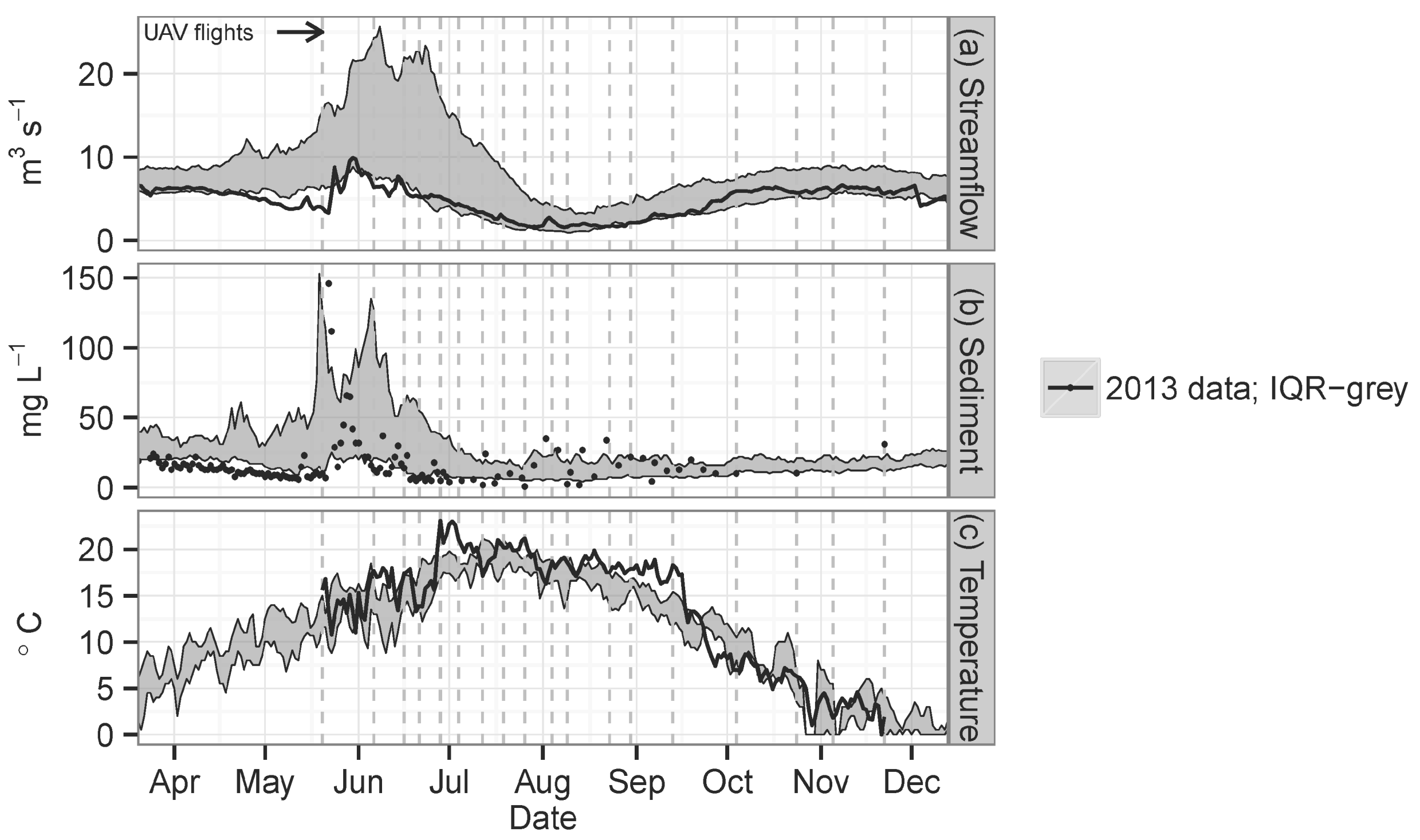
2.5. Data Acquisition Missions

Aerial surveys were completed roughly every two weeks over the active channel [2], or more frequently as river conditions necessitated, with a total of 18 different flights over the summer of 2013 (20 May 2013–22 November 2013). Because passive radiation (sunlight) must pass through the intervening water column, reflect off the bottom, and then back through the water column to the UAV sensor for optical imaging (i.e., radiation in the visible region), the reflectance reaching the image sensor at a given wavelength depends on the volume attenuation characteristics of the water. Attenuation is a function of the thickness of the water layer and its absorption and scattering properties (e.g., color, organic and inorganic suspended material, etc.) [18].

In rivers, volume attenuation is related to streamflow stage and suspended sediment concentration, the latter of which is probably most important in shallow systems where depths are often <1 m. To characterize the optical characteristics of the water, total suspended sediment samples were collected biweekly using Equal Width Increment (EWI) procedures with a US DH-48 sampler [48], or by grab sampling. Samples were analyzed via standard method 2540-E for examination of water and wastewater [49]. At the same time, light attenuation profiles were measured with a Li-COR 192 (Lincoln, NB) quantum meter at incremental depths of 0.1 m so that the overall light extinction coefficient (k_e) of the water could be determined. Finally, daily streamflow and subweekly suspended sediment samples were compiled for the USGS streamgaging station 12324200 Clark Fork at Deer Lodge MT [50] to provide a consistent measure of the optical transparency of the water.

UAV missions were scheduled according to Fleming [51] and Mount [52] to avoid the sun’s reflection (glitter or glint) from water surfaces, which can seriously diminish the amount of detail in underwater imagery. Flights were conducted midmorning or early evening under the Model Aircraft Operating Standards Advisory Circular (AC) 91–57, and did not require a Federal Aviation Administration (FAA) Certificate of Authorization (COA). This was because the primary author (K.F.) was the owner and operator of the flight and imaging system, and no compensation or grant funding was provided for its use [53]. AC 91–57 specifically excludes UAV operation for business purposes [40], therefore readers should consult current government regulations before initiating their own studies. Notably, a widespread hurdle still exists with UAV use—federal regulation [35,41].

Prior to the flights, horizontal control points at the site were established by positioning six aerial ground targets (48" × 48" PVC iron cross style) at known benchmarks (wooden survey hubs) spaced throughout the river corridor. These were surveyed with a SonTek real time kinematic (RTK) global positioning system (GPS) linked with a separate base station so a horizontal position accuracy of ±3 cm could be achieved (WGS 84). Control was verified using a National Geodetic Survey benchmark approximately one kilometer from the site, and eight other distinctive objects or control points (e.g., large immovable rocks, salient features, etc.) were also benchmarked as described by others [54].

Before the initial flight (20 May 2013), the compass of the Naza-M autopilot system was calibrated to local magnetic conditions as described by the manufacturer [55]. The purpose of this calibration was to improve the UAV heading accuracy. Thereafter, the UAV was operated by remote control during each reconnaissance mission. To track altitude above ground level (AGL), a Leica Geovid 10 × 42 HD rangefinding binocular was used. Height was measured approximately every 15–20 s until the maximum altitude AGL of 120 m was achieved. Thereafter the GPS was used to hold position vertically.

The camera was activated manually upon takeoff and digital images were taken every 2–5 s on autoexposure depending on mission conditions using the camera’s time-lapse feature (i.e., intervalometer). Flights took less than 10 min for the study reach (one-km), and 100–250 images were obtained during each mission to ensure that sufficient coverage of the project site was attained. Flights were often, but not always, conducted with an observer to improve safety.

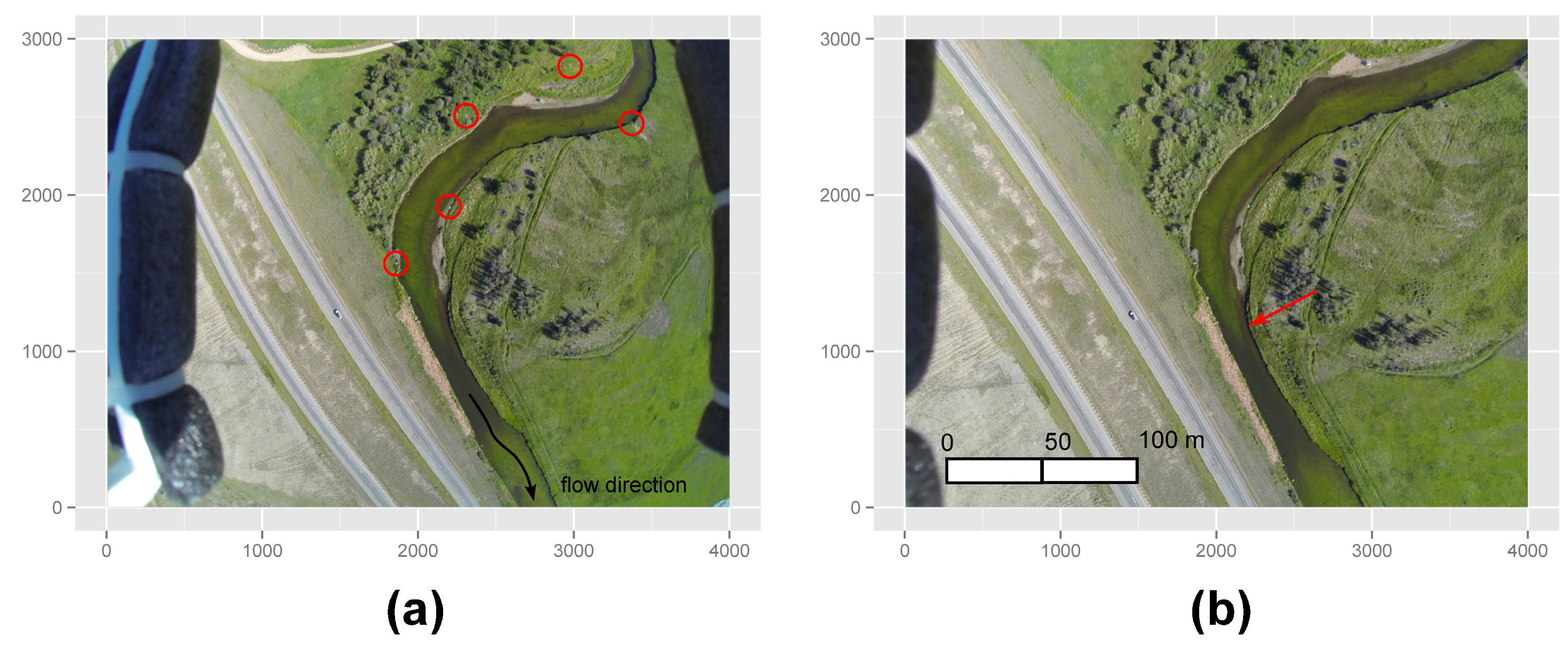
2.6. Ground-Based Verification of Remote Sensing Results

Ground truth data were collected to verify the remote sensing results on 21 June 2013, a time when algal coverage was near maximal. The one-kilometer segment was surveyed visually by wading the entire river, noting the presence of algal cover relative to that observed on aerial images. Cover was easy to distinguish, and we used circumspect observations to digitize a polygon shapefile of Cladophora coverage using a georeferenced air photo for reference. This was later rasterized at a resolution of 0.25 m to compute the remote sensing statistics described subsequently. Ground measurements were deemed valid for several weeks within the date of the survey, and therefore represent a snapshot of algal cover over the study reach at the time.

2.7. Geometric Correction

The use of a fisheye lens for aerial photography requires precise knowledge about intrinsic camera parameters including the focal distance, principal point coordinates, and the lens distortion function. A useful strategy for camera calibration is provided by several investigators [56,57], which requires observing a series of planar checkerboard calibration patterns to fit a generic camera model. For fisheye calibration, the equidistance projection is commonly used, which takes the form [56]

$$r=f\theta$$

(1)

where r is the radially projected distance between the image point and the principal point (principal point being the center of the lens, mm), θ is the angle between the principal axis and the incoming ray (radians), and f is the camera focal length (mm). In the equidistant model, the unit area per pixel in the image decreases from the principal point outward.

Because real lenses do not precisely follow the theoretical equation, a more generic constrained polynomial model was employed [57]

$$r\left(\theta \right)=\theta +k_1{\theta }^3+k_2{\theta }^5+k_3{\theta }^7+k_4{\theta }^9$$

(2)

where k₁, k₂, k₃, and k₄ are distortion coefficients that satisfy minimization of least squares between the observed and predicted coordinates. It should be noted that other forms of the polynomial have been reported elsewhere [41,56].

The above model was implemented in the Matlab^® Camera Calibration Toolbox [57,58]. Calibration was completed by taking 20 images of a 50.8 mm checkerboard pattern affixed to a 508 mm × 762 mm sheet of poster board at different perspectives, and then using the software to implement iterative solutions between observed and predicted corner points until the model distortion coefficients were optimized. No radiometric corrections were made to adjust for vignetting (none was observed), and this region is clipped anyway during the Matlab^® processing. Consequently, images can be treated as conventional pictures taken from a perspective camera [41].

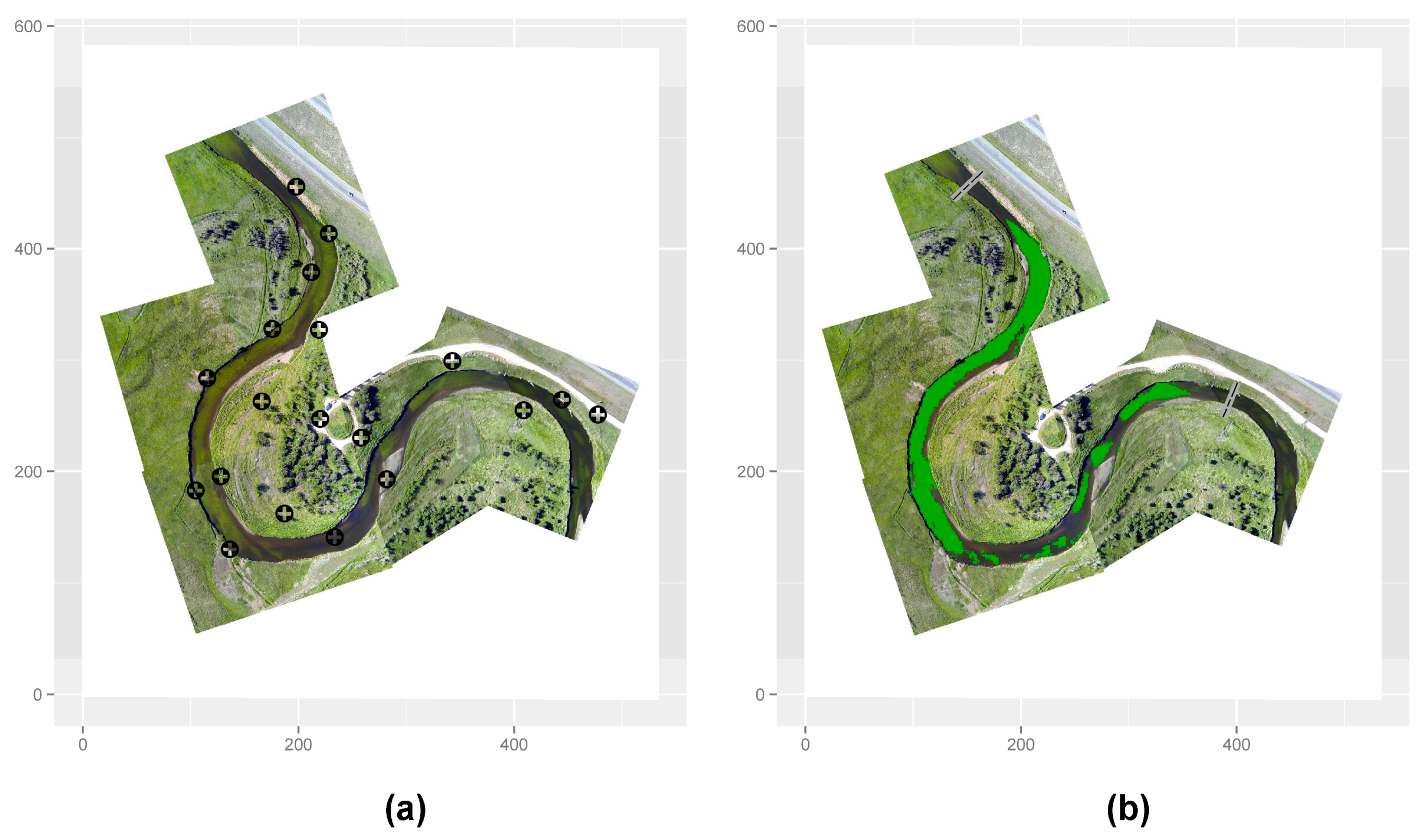
2.8. Georeferencing and Mosaicking

We used ArcGIS for mosaicking and georeferencing. Only images with minimal tilt displacement were selected. We also omitted relief displacement given the lack of topography in the project area. In this regard, images are very close to planimetrically correct (i.e., orthorectified). Mosaics were stitched together using overlapping points within ArcGIS, and affine and higher-order polynomial transformations including spline and adjust were used to georeference the mosaicked image to observed control points (i.e., the surveyed targets/fixed immovable objects described previously). Descriptions of these methods are found in ESRI [59].

2.9. Image Analysis and Algal Mapping

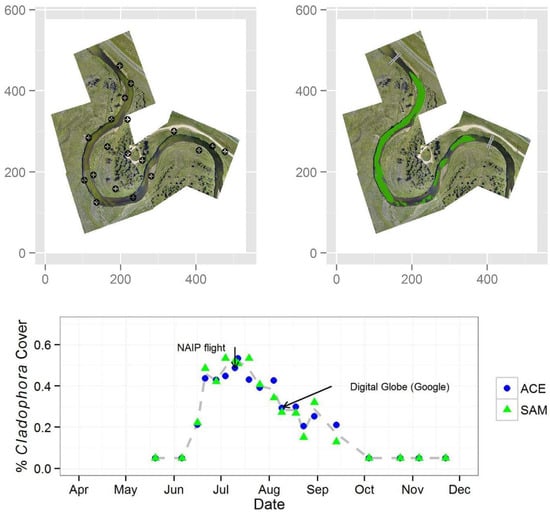
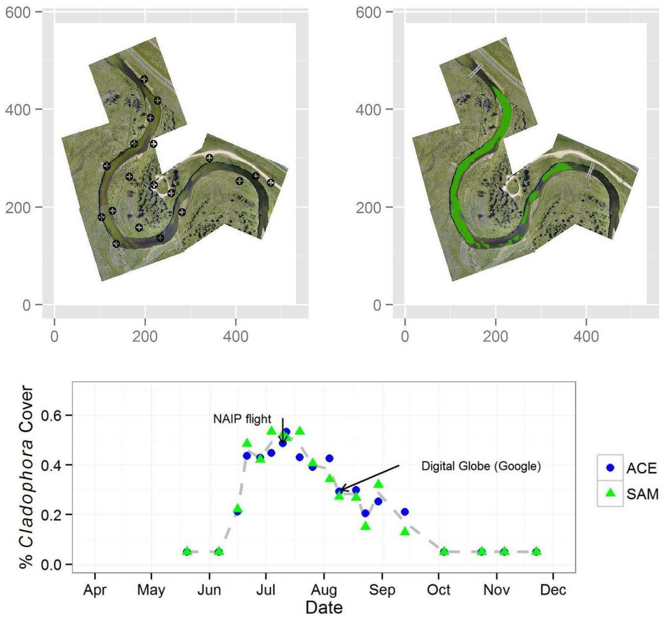
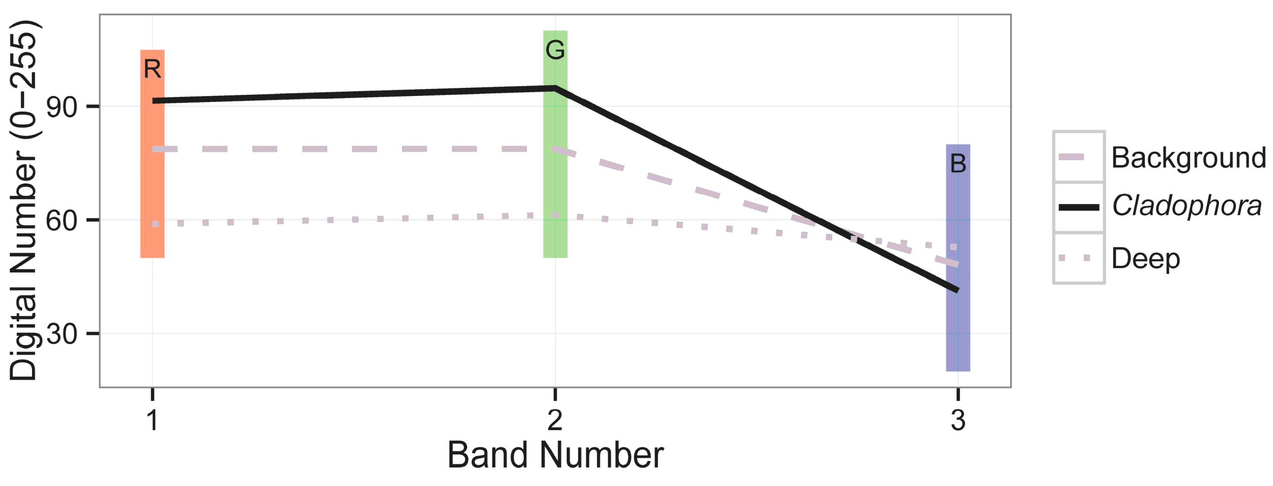
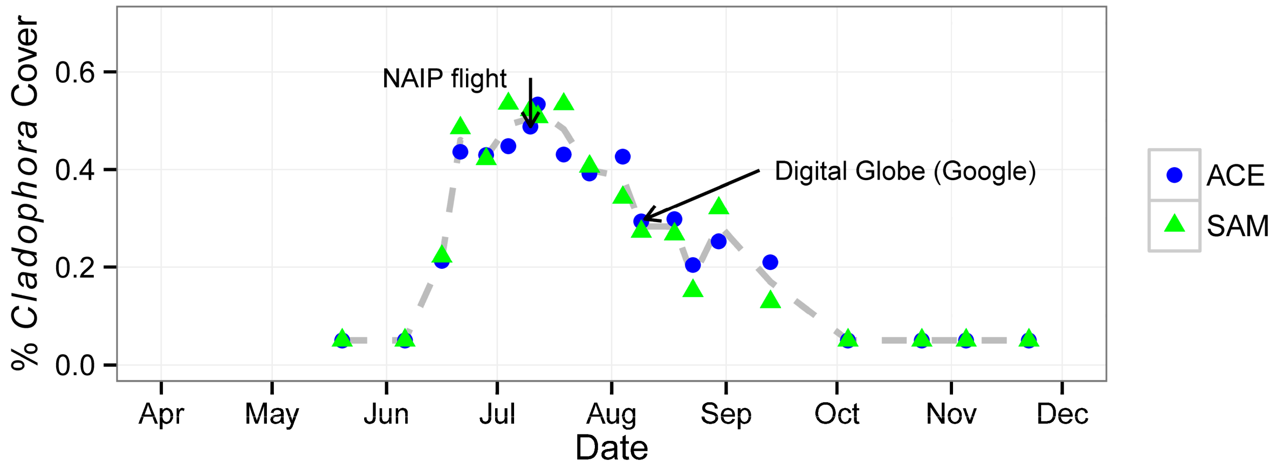
Once images were georeferenced, classification of Cladophora spatial cover was completed with an adaptive cosine estimator (ACE) and spectral angle mapper (SAM) algorithm. The public domain software Opticks version 4.11.0 was used in conjunction with the spectral processing extension (version 1.8.0) [60]. ACE is a statistical method useful in differentiating notably green Cladophora from native substrate or golden-hued diatom periphyton of the river bottom. SAM is a non-statistical method that makes direct comparisons of spectra with a known end member. The Cladophora spectral signature during each flight was determined by completing supervised classification of a region that was known to contain Cladophora during each mission.

The efficacy of remote sensing was judged by the tau coefficient (T), which is a commonly used index that determines the percentage of the pixels that were classified correctly beyond that which would be expected by chance alone. T is calculated as [61,62]

$$T=\frac{P_0-P_r}{1-P_r}$$

(3)

where P₀ is the overall percentage agreement, i.e., the sum of the diagonal value in the error matrix divided by the total number of observations [63], and P_r is the random probability of agreement that a pixel for a given habitat would be classified correctly by chance (e.g., Cladophora or background in this application) [61,62]

$$P_r=\frac{1}{N^2}{\displaystyle \sum }_{i=1}^M{n}_i{x}_i$$

(4)

where M is the number of habitat types, i is the i^th habitat type, x_i is the diagonal value for habitat i in the error matrix (i.e., the number of correct assignments), and n_i is the row total for habitat i in the error matrix. T was calculated for a single imaging period consistent with the ground truth surveys.

3. Results

Environmental conditions encountered during 2013 are shown in Figure 4. Streamflow was below normal most of the year (near the 25th percentile) with daily suspended sediment concentration averaging 10–30 mg∙L⁻¹ in winter (October–May), peaking near 150 mg∙L⁻¹ during spring freshet (late May), and <10 mg∙L⁻¹ during the low flow period. Consequently, neither suspended sediment nor river turbidity were likely a factor affecting algal growth or volume attenuation during most of the UAV imaging timeframe (k_e = 0.5‒1.7 m⁻¹; n = 6). Water temperatures were also supportive of Cladophora growth, staying well above the limiting threshold of 5 °C [9] until late October.

Figure 4. Conditions encountered during the 2013 unmanned aerial vehicle studies. (a) Mean daily streamflow; (b) Instantaneous suspended sediment concentration; and (c) Mean daily water temperature. The imaging dates are denoted by dashed vertical lines and the interquartile range (IQR) for each constituent is shown over the period of record (1979–2013) in grey.

Figure 4. Conditions encountered during the 2013 unmanned aerial vehicle studies. (a) Mean daily streamflow; (b) Instantaneous suspended sediment concentration; and (c) Mean daily water temperature. The imaging dates are denoted by dashed vertical lines and the interquartile range (IQR) for each constituent is shown over the period of record (1979–2013) in grey.

Unprocessed and calibrated UAV images acquired near peak Cladophora growth (28 June 2013) are shown in Figure 5. Ground targets are highlighted in red (Figure 5a), and images have not yet been georeferenced or rectified. When comparing the unprocessed (Figure 5a) and calibrated image (Figure 5b), it should be noted that the edges have been clipped, which is an automated feature of the Matlab^® Camera Calibration Toolbox [57].

Figure 5. Example images captured with the unmanned aerial vehicle (UAV) imaging system. (a) Unprocessed image showing full distortion, where legs of the UAV are apparent and ground targets are highlighted in red (circled). Units are in pixels; (b) calibrated image from the Matlab^® Camera Calibration Toolbox [57], where resolution decreases towards the outside edge. The red arrow denotes a spatial feature of interest, as described in the text.

Figure 5. Example images captured with the unmanned aerial vehicle (UAV) imaging system. (a) Unprocessed image showing full distortion, where legs of the UAV are apparent and ground targets are highlighted in red (circled). Units are in pixels; (b) calibrated image from the Matlab^® Camera Calibration Toolbox [57], where resolution decreases towards the outside edge. The red arrow denotes a spatial feature of interest, as described in the text.

As illustrated in Figure 5 (and Figure 6 later), Cladophora is spatially patchy. Accordingly, the channel ranges from being nearly devoid, to nearly 100% covered with SAV. Structural features of interest include the V-shaped feature at the bottom of Figure 5b (red arrow, which is a riffle with a pronounced velocity increase), and then slow-moving water in adjoining segments (i.e., the sides of the channel and pool downstream), which are conspicuously devoid of SAV. The relationship between water velocity (current) and algal cover is a topic of current research at the site.

Lens calibration results for the undistorted image are shown in Table 1. Overall, the calibration had an error of ~1.25 pixels, meaning that a raster with 0.25 m resolution (as shown in Figure 5) has an average spatial error of ±0.3 m prior to georeferencing. Hence a fairly precise calibration was achieved that yields reliable pixel translation through the equidistance projection (Equation (2)).

Table 1. Results of the GoPro Hero 3 camera calibration using the Matlab^® Camera Calibration Toolbox [57]. The horizontal angle of view was determined to be 129°, which at an altitude of 120 m covers an area just over 500 m horizontally (375 m vertically).

Attribute	Fitted Value		Uncertainty (±) a
	X	Y
Focal length (pixels)	1782.384	1782.453	3.257	3.277
Principle point	1967.203	1449.815	1.839	1.276
Pixel error	1.23959	1.25056	---
Distortion
k1	−0.03606		0.00660
k2	0.11243		0.02028
k3	−0.03936		0.02475
k4	0.00198		0.01019

^a The numerical uncertainty is approximately three times the standard deviation.

Table 1. Results of the GoPro Hero 3 camera calibration using the Matlab^® Camera Calibration Toolbox [57]. The horizontal angle of view was determined to be 129°, which at an altitude of 120 m covers an area just over 500 m horizontally (375 m vertically).

Attribute	Fitted Value		Uncertainty (±) a
	X	Y
Focal length (pixels)	1782.384	1782.453	3.257	3.277
Principle point	1967.203	1449.815	1.839	1.276
Pixel error	1.23959	1.25056	---
Distortion
k1	−0.03606		0.00660
k2	0.11243		0.02028
k3	−0.03936		0.02475
k4	0.00198		0.01019

^a The numerical uncertainty is approximately three times the standard deviation.

Images that are mosaicked and georeferenced provide a more comprehensive understanding of river and plant behavior. For example; one meander length of the river is tiled together in Figure 6 for the same period of peak growth depicted in Figure 5. In this case; spatial algal structure is noted at multiple locations: notably; the V-shaped feature mentioned previously; an expansive area of Cladophora cover in the thalweg of the river (i.e., where the bulk of the water is flowing in the channel); and several patchy “islands” on the right side of the image. Algal accumulation is prevalent in some locations, but inconspicuous in others, implying existence of habitat preference as discussed later (see Discussion).

General statistics for the tiled mosaic (i.e., Figure 6) clipped to the river corridor, with the target spectra removed (Cladophora), are shown in Table 2. The tabulated band means suggest there is more reflectance in the red and green spectral region than the blue band, which indicates wavelength-specific attenuation of light is not of great importance in this river. Otherwise a greater percentage of blue intensity would have been observed (i.e., red and green are preferentially absorbed over blue in deep water). This can be confirmed by review of the variance-covariance matrix in Table 2.

Figure 6. (a) Mosaicked and georeferenced unmanned aerial vehicle images showing one meander length of the Clark Fork River and aerial targets. Units are in meters; (b) adaptive cosine estimator classification results (green shading) for Cladophora based on a threshold percentage of 0.80. The analysis extent for each mapping mission was limited to the area between the grey hashmarked lines.

Figure 6. (a) Mosaicked and georeferenced unmanned aerial vehicle images showing one meander length of the Clark Fork River and aerial targets. Units are in meters; (b) adaptive cosine estimator classification results (green shading) for Cladophora based on a threshold percentage of 0.80. The analysis extent for each mapping mission was limited to the area between the grey hashmarked lines.

Table 2. Calculated band mean and variance-covariance matrix for the 28 June 2013 unmanned aerial vehicle image mosaic. Values are for the image background after the target was removed.

	μi	Band 1 (Red)	Band 2 (Green)	Band 3 (Blue)
Band 1 (red)	78.73604237543	276.1323309468	271.4320405892	224.5080967758
Band 2 (green)	78.76149526543	271.4320405892	291.3337301972	8.384664633906
Band 3 (blue)	48.16133256564	224.5080967758	8.384664633906	103.5271385886

Table 2. Calculated band mean and variance-covariance matrix for the 28 June 2013 unmanned aerial vehicle image mosaic. Values are for the image background after the target was removed.

	μi	Band 1 (Red)	Band 2 (Green)	Band 3 (Blue)
Band 1 (red)	78.73604237543	276.1323309468	271.4320405892	224.5080967758
Band 2 (green)	78.76149526543	271.4320405892	291.3337301972	8.384664633906
Band 3 (blue)	48.16133256564	224.5080967758	8.384664633906	103.5271385886

Details on the spectral signatures of interest (e.g., Cladophora, river background, etc.) are provided in Figure 7. In this case, the target spectrum (Cladophora), image background (diatoms and bare substrate), and optically deep water are all different. Cladophora reflect more green and red than either of the other two classes (see magnitude of digital number for support of this statement), which is consistent with reported reflectance ratios in the literature [25,64,65]. It is important to note that the spectrum in Figure 7 will change according to lighting conditions, algal condition, or optical clarity of the river water. Consequently the intensity of the digital number for Cladophora will vary, but the ratio of the bands should scale consistently.

Figure 7. Spectral signals for Cladophora, river background (i.e., diatoms or bare substrate), and optically deep water for the 28 June 2013 unmanned aerial vehicle image mosaic. The reflectance for Cladophora was highest in the green band (band number 2) followed by red (band number 1), and then blue (band number 3). The digital number reflects the intensity of reflectance in each band from 0 to 255.

Figure 7. Spectral signals for Cladophora, river background (i.e., diatoms or bare substrate), and optically deep water for the 28 June 2013 unmanned aerial vehicle image mosaic. The reflectance for Cladophora was highest in the green band (band number 2) followed by red (band number 1), and then blue (band number 3). The digital number reflects the intensity of reflectance in each band from 0 to 255.

The error matrix and Tau (Τ) for the ACE and SAM classification procedure are shown in Table 3. A visual comparison of the ACE results is shown in Figure 6b. Classifications are highly accurate with an overall accuracy (P₀) of approximately 90% and 92%, which yield Τ (Equation (3)) of 0.82 and 0.84 for ACE and SAM, respectively. In this case, ACE was slightly less accurate than SAM in Cladophora classification, but was much less sensitive to threshold value. As a consequence, both ACE and SAM appear to provide reasonably reliable and consistent identification of Cladophora. Results comparatively are on par with literature studies in lakes and estuaries e.g., [18,19,20] and could likely be improved through iterative refinement of the threshold value (i.e., 0.8 for ACE and 5° for SAM).

Table 3. Error matrix and calculated tau coefficients (Τ) for the adaptive cosine estimator (ACE) and spectral angle mapper (SAM) classifications of Cladophora on the Clark Fork. Calculations are for the 28 June 2013 unmanned aerial vehicle image mosaic. The reference data come from digitized areas of known Cladophora, which were identified through aerial photo interpretation and associated ground truth.

	ACE (Threshold of 0.80)		SAM (Spectral Angle of 5°)
	Cladophora	Background	Cladophora	Background
Cladophora	94,380	9057	94,904	6504
Background	13,769	120,907	13,245	123,460
overall accuracy = 90%, Τ = 0.82			overall accuracy = 92%, Τ = 0.84

Table 3. Error matrix and calculated tau coefficients (Τ) for the adaptive cosine estimator (ACE) and spectral angle mapper (SAM) classifications of Cladophora on the Clark Fork. Calculations are for the 28 June 2013 unmanned aerial vehicle image mosaic. The reference data come from digitized areas of known Cladophora, which were identified through aerial photo interpretation and associated ground truth.

	ACE (Threshold of 0.80)		SAM (Spectral Angle of 5°)
	Cladophora	Background	Cladophora	Background
Cladophora	94,380	9057	94,904	6504
Background	13,769	120,907	13,245	123,460
overall accuracy = 90%, Τ = 0.82			overall accuracy = 92%, Τ = 0.84

It is also of interest to extend the classifications temporally (i.e., compare multiple images). An animated version of 18 scenes acquired as part of this investigation is shown in Supplemental File 1 using the ACE classification technique. In this instance, Cladophora cover is mapped spatially from the beginning to the end of the growing season (May–November) and includes two non-UAV images (20 total) from the National Agriculture Imagery Program (NAIP) and DigitalGlobe (Google Earth).

Accordingly, it is seen that: (1) rapid Cladophora accumulation occurs following vernal freshet; (2) steady-state conditions prevail for much of the early summer; and (3) finally senescence and sloughing begin during late summer. Ultimately a shift to a diatom conglomerate occurs in the fall/early winter, which could not be discerned via optical imaging. When viewing Supplementary File 1, it is important to note that Cladophora may not be optically visible during initial colonization or succession, but may still be present under the water surface. This was noted in several instances where cover was estimated as <5% (shown as 5%). In these cases, filaments were often less than 2 cm.

Tabulated percent cover values (reach wide) for image dates consistent with this animation are shown in Table 4 along with the threshold levels needed to achieve those results. ACE was quite stable (value of 0.8 for all images) whereas SAM was highly variable. The discrepancy between these two techniques is unclear, but is thought to be related to quality of image and exposure, and streamflow and suspended sediment concentration. Higher angular differences are perhaps needed to appropriately discriminate Cladophora in clear water (low sediment) than under turbid conditions using SAM. This result is counterintuitive, but suggests turbidity influences the sensitivity of the results. Percent cover estimates for both ACE and SAM are shown in Figure 8.

Table 4. Results of Cladophora algal cover mapping over the analysis period. Streamflow and suspended sediment concentration (SSC) are also shown.

Date	Attribute
	% Cladophora Cover		Threshold		Streamflow (m3∙s−1)	SSC d (mg∙L−1)
	ACE	SAM	ACE	SAM
20 May 2013	<0.05 a	<0.05 a	—	—	3.91	10
6 June 2013	<0.05 a	<0.05 a	—	—	6.37	13
16 June 2013	0.21	0.22	0.80	2	6.46	16 (14)
21 June 2013	0.44	0.48	0.80	3	5.24	7
28 June 2013	0.43	0.42	0.80	5	5.24	5 (2)
4 July 2013	0.45	0.53	0.80	7	4.39	5
10 July 2013 b	0.49	0.52	0.80	5	3.43	7
12 July 2013	0.53	0.51	0.80	3	3.40	25 (2)
19 July 2013	0.43	0.53	0.80	3	2.75	11
26 July 2013	0.39	0.41	0.80	2.5	1.81	11 (<1)
4 August 2013	0.43	0.34	0.80	2	2.41	23
9 August 2013	0.29	0.27	0.80	1.5	1.61	19 * (3)
18 August 2013 c	0.30	0.27	0.80	3	1.87	14
23 August 2013	0.20	0.15	0.80	3	1.67	33 *
30 August 2013	0.25	0.32	0.80	1.5	2.15	21
13 September 2013	0.21	0.13	0.80	1	2.92	13 *
4 October 2013	<0.05 a	<0.05 a	—	—	6.06	(10)
24 October 2013	<0.05 a	<0.05 a	—	—	6.03	(11)
5 November 2013	<0.05 a	<0.05 a	—	—	6.12	—
22 November 2013	<0.05 a	<0.05 a	—	—	5.58	(31)

^a Cladophora was not visible or was not present on these dates; ^b National Agriculture Imagery Program (NAIP) photo (1 m resolution); ^c Digital Globe satellite image (0.5 m resolution); ^d U.S. Geological Survey (USGS) value (site sample in parentheses); * ±2 days from image.

Table 4. Results of Cladophora algal cover mapping over the analysis period. Streamflow and suspended sediment concentration (SSC) are also shown.

Date	Attribute
	% Cladophora Cover		Threshold		Streamflow (m3∙s−1)	SSC d (mg∙L−1)
	ACE	SAM	ACE	SAM
20 May 2013	<0.05 a	<0.05 a	—	—	3.91	10
6 June 2013	<0.05 a	<0.05 a	—	—	6.37	13
16 June 2013	0.21	0.22	0.80	2	6.46	16 (14)
21 June 2013	0.44	0.48	0.80	3	5.24	7
28 June 2013	0.43	0.42	0.80	5	5.24	5 (2)
4 July 2013	0.45	0.53	0.80	7	4.39	5
10 July 2013 b	0.49	0.52	0.80	5	3.43	7
12 July 2013	0.53	0.51	0.80	3	3.40	25 (2)
19 July 2013	0.43	0.53	0.80	3	2.75	11
26 July 2013	0.39	0.41	0.80	2.5	1.81	11 (<1)
4 August 2013	0.43	0.34	0.80	2	2.41	23
9 August 2013	0.29	0.27	0.80	1.5	1.61	19 * (3)
18 August 2013 c	0.30	0.27	0.80	3	1.87	14
23 August 2013	0.20	0.15	0.80	3	1.67	33 *
30 August 2013	0.25	0.32	0.80	1.5	2.15	21
13 September 2013	0.21	0.13	0.80	1	2.92	13 *
4 October 2013	<0.05 a	<0.05 a	—	—	6.06	(10)
24 October 2013	<0.05 a	<0.05 a	—	—	6.03	(11)
5 November 2013	<0.05 a	<0.05 a	—	—	6.12	—
22 November 2013	<0.05 a	<0.05 a	—	—	5.58	(31)

^a Cladophora was not visible or was not present on these dates; ^b National Agriculture Imagery Program (NAIP) photo (1 m resolution); ^c Digital Globe satellite image (0.5 m resolution); ^d U.S. Geological Survey (USGS) value (site sample in parentheses); * ±2 days from image.

Figure 8. Estimated algal cover for 18 unmanned aerial vehicle (UAV) imaging missions over the summer of 2013 on the Clark Fork River (average of one-km reach). Digital classifications for both the adaptive cosine estimator (ACE) and spectral angle mapper (SAM) are shown for the following image sources: 18 UAV flights, the 10 July 2013 National Agriculture Imagery Program (NAIP) flight, and the 18 August 2013 Digital Globe coverage from Google Earth. Cover increases quickly following freshet, peaks in early July, and recedes for the remaining part of the summer and early fall.

Figure 8. Estimated algal cover for 18 unmanned aerial vehicle (UAV) imaging missions over the summer of 2013 on the Clark Fork River (average of one-km reach). Digital classifications for both the adaptive cosine estimator (ACE) and spectral angle mapper (SAM) are shown for the following image sources: 18 UAV flights, the 10 July 2013 National Agriculture Imagery Program (NAIP) flight, and the 18 August 2013 Digital Globe coverage from Google Earth. Cover increases quickly following freshet, peaks in early July, and recedes for the remaining part of the summer and early fall.

4. Discussion

Based on the results above, remote sensing of river algae by small-scale UAVs is a viable and potentially valuable research tool. In particular, UAV platforms offer the ability to provide high-resolution sub-meter data at a frequency greater than traditional techniques such as satellites or dedicated aircraft. In some situations, they may even provide quasi-continuous coverage of dynamic river environments. As such, UAVs are a suitable tool for SAV mapping and other river research. A number of considerations should be made prior to initiating UAV benthological studies, however.

4.1. UAV Use in Freshwater Benthic Ecology

It has been suggested by some that there is a steep learning curve associated with UAV operation [35]. While this may be true in some cases, our experience is that this initial effort is not insurmountable. For example, with no prior knowledge of aviation, the primary author (K.F.) was able to achieve satisfactory control over the aircraft within several hours of airworthiness trials and was comfortable with the imaging results shortly thereafter. This may be a distinct advantage of small UAVs; they are available to any researcher willing to invest the initial effort.

However, a number of other factors should be considered beyond operational simplicity. These include aircraft safety, payload and stability limitations, flight capabilities, and the type of imaging sensor. Nearly all of these topics are described by other researchers with respect to remotely piloted vehicles [35,36,37,47]. For this reason, we emphasize the primary benefit of UAV to ecologists—added flexibility in flight planning and capability to deliver high-resolution digital images. Rivers are dynamic systems (Figure 4) that operate on fine spatial scales (Figure 5 and Figure 6). They need to be monitored repeatedly to understand transient physical and biological processes. Accordingly, UAV reconnaissance is a suitable technique for monitoring fluvial phenomena such as algal colonization, peak algal cover, and algal sloughing as demonstrated in this study. It would be difficult to obtain such rich spatial and temporal data without them.

However, limitations of UAVs must also be considered. Two primary factors were noted in this work. One is wind turbulence and off-nadir images, which are common with such aircraft [37]. To mitigate this first consideration, photographs were oversampled and we recommended an exposure be taken every 2–5 s so those with acceptable geometry can be retained. The other is the optical environment, which greatly affects the spectrum of SAV. Ambient lighting and meteorological conditions result in inconsistent spectral signatures across different UAV flights, hence the signature presented in Figure 7 is unique to that flight. Procedures for radiometric adjustment of the digital image for atmospheric correction could potentially be applied [25], however, changes in turbidity, water depth, and plant physiological condition further obfuscate the spectral response [66] making remote sensing of rivers a challenging endeavor [2].

Potential improvements to the methods described here are widespread; included are the use of fixed wing platforms for increased efficiency and coverage, waypoint navigation for mission repeatability, and enhanced imaging techniques. For example, the UAV used in this work now incorporates an iPad ground station for waypoint flight, on-screen route planning, and near autonomous operation. A number of other commercial off-the-shelf autopilots are also available. Beyond flight-oriented improvements, the use of high-quality gimbals for camera stabilization, or more robust camera sensors (e.g., multispectral or hyperspectral), are further considerations for improving techniques described herein.

One word of caution with UAV is that government restrictions may limit their use [35]. Readers are encouraged to seek current regulations when planning a study. In our work, we were limited to a flight ceiling of 120 m (just below 400 feet), which influences the number of images required for coverage of a given area. For UAV research activities similar to those described in this paper, a wide-angle lens will undoubtedly be needed to capture an area appropriate image area [41]. Cameras with a horizontal field of view exceeding 120° are recommended, or additional workload in calibrating, rectifying, georeferencing, and mosaicking a large number of images may be required. The added burden may very well offset the initial cost-benefit of UAVs [34].

When compared to other methods, the algal mapping described herein is still relatively low cost. For example, each one-km long scene described here (18 total scenes) had an estimated cost of $500–$600 U.S. dollars, which includes the purchase cost of the UAV and camera system, base Matlab^® package, student ArcView license (with Spatial Analyst), ground control surveys (including RTK rental), image acquisition, distortion removal, stitching and georeferencing images, and data processing (8 h labor per scene). The estimate does not include the initial camera calibration or spectral analysis. When defrayed over multiple years, and for small project sites of several square kilometers, UAVs are still considerably cheaper. Minimum orders for most commercial satellites are currently >US$2500 [20] and do not become cost-effective until spread out over larger areas [32].

4.2. Understanding Cladophora Behavior through UAV Remote Sensing

We documented accrual, peak, and autogenic sloughing of Cladophora over the growing season using a UAV (Figure 8). A similar progression of short-term biomass accrual (and loss) has been described elsewhere [67]. Thus the results were expected. However, rarely has the spatial extent been characterized to the degree described here (i.e., Supplemental File 1). Consequently, UAV reconnaissance provides an important contribution to benthological research, one that may be useful in recording changes in water quality over time, spatial differences due to alternative management actions, or understanding critical events such as sloughing. Methods could perhaps be extended to other species, or be adapted to annual monitoring programs as a measure of stream health [25]. In this regard, our article presents a useful contribution to mapping benthic algae in freshwater ecosystems. However, the need for research on both flight systems and digital imaging procedures is still warranted and recommended.

Nonetheless, UAV may help shed light on a number of topics that have eluded researchers for many years. For example, determining Cladophora habitat preference [68,69] (Figure 5 and Figure 6), understanding physical interactions between velocity, substrate, and scouring flows in regulated rivers [70], algal sloughing following stream spates [71,72], or causes of algal spatial patchiness [72] may all be better described with detailed remote sensing measurements than traditional observation techniques. Similarly, temporal studies of algal cover could be paired with quantitative measures of in situ dissolved oxygen, or acoustic Doppler current profiler data, to relate algal cover (or biomass) with instream primary productivity or river velocity. Moreover, rapid UAV deployments may afford the opportunity to analyze real time problems such as two-dimensional mixing (lateral and longitudinal) or velocity using optically visible dyes. In this regard, research topics with UAV are abounding.

As a final point, the growing repository of historical optical imagery over inland freshwaters may be a useful resource in backfilling our knowledge about SAV or algal cover changes over time. High resolution color aerial photography can now be obtained from a number of sources (see Google Earth, latitude 46.4981°, longitude −112.7414° for a chronology of this project site) and the approach described in this article may be useful for identifying commonalities in annual spatial structure, time-lagged effects, or perhaps scouring flows required to prevent nuisance algae. Changes in water quality, or the influence of management actions on algal cover over time, could also potentially be elucidated.

5. Conclusions

An approach for remote sensing and mapping of filamentous algal accumulations in clear shallow rivers is presented using an inexpensive unmanned aerial vehicle (UAV). For under US$1500, a lightweight and rapid response aerial imaging system can be developed that provides spatially precise (±0.3 m horizontal position) and high-resolution (0.25 m) characterization of benthic phenomenon. Advantages of UAVs are numerous, but flexibility in flight planning and the ability to conduct repeat missions (18 total) were of greatest benefit in this study. Accordingly, we gained an enhanced understanding of the submerged aquatic vegetation Cladophora glomerata including locations of spatial habitat preference (via image correction, georeferencing, and mosaicking) and changes in algal cover over time (through sequential imaging of colonization, exponential growth, and autogenic sloughing). Each is of ecological significance to gaining a better understanding algal dynamics in flowing water. Consequently, we believe a significant opportunity exists for applying UAVs to other ecological investigations in freshwater river environments. Future studies should seek to provide more robust information including algal biomass or relationships between algal cover and biotypes such as riffles, pools, or glides. Advances may also be made by combining UAV reconnaissance with other investigative techniques such as in situ velocity profiling or measurement of substrate and other limiting factors.

References

1. Dennison, W.C.; Orth, R.J.; Moore, K.A.; Stevenson, J.C.; Carter, V.; Kollar, S.; Bergstrom, P.W.; Batiuk, R.A. Assessing water quality with submersed aquatic vegetation. BioScience 1993, 43, 86–94. [Google Scholar] [CrossRef]
2. Marcus, W.A.; Fonstad, M.A.; Legleiter, C.J. Management applications of optical remote sensing in the active river channel. In Fluvial Remote Sensing for Science and Management; Carbonneau, P.E., Piégay, H., Eds.; John Wiley & Sons, Ltd.: Chichester, UK, 2012; pp. 19–41. [Google Scholar]
3. Carpenter, S.R.; Lodge, D.M. Effects of submersed macrophytes on ecosystem processes. Aquat. Bot. 1986, 26, 341–370. [Google Scholar] [CrossRef]
4. Janauer, G.; Dokulil, M. Macrophytes and algae in running waters. In Biological Monitoring of Rivers; Ziglio, G., Siligardi, M., Flaim, G., Eds.; John Wiley & Sons, Ltd.: Chichester, UK, 2006; pp. 89–109. [Google Scholar]
5. U.S. Environmental Protection Agency (USEPA). Submerged aquatic vegetation. In Volunteer Estuary Monitoring: A Methods Manual; Ohrel, R.L., Registar, K.M., Eds.; Ocean Conservancy: Washington, DC, USA, 2006; pp. 1–16. [Google Scholar]
6. Duarte, C.M. Submerged aquatic vegetation in relation to different nutrient regimes. Ophelia 1995, 41, 87–112. [Google Scholar] [CrossRef]
7. Torn, K.; Martin, G. Response of submerged aquatic vegetation to eutrophication-related environment descriptors in coastal waters of the NE Baltic Sea. Est. J. Ecol. 2012, 61, 106–118. [Google Scholar] [CrossRef]
8. Blum, J.L. The ecology of river algae. Bot. Rev. 1956, 22, 291–341. [Google Scholar] [CrossRef]
9. Whitton, B.A. Biology of Cladophora in freshwaters. Water Res. 1970, 4, 457–476. [Google Scholar] [CrossRef]
10. Dodds, W.K.; Gudder, D.A. The ecology of Cladophora. J. Phycol. 1992, 28, 415–427. [Google Scholar] [CrossRef]
11. Ensminger, I.; Hagen, C.; Braune, W. Strategies providing success in a variable habitat: I. Relationships of environmental factors and dominance of Cladophora glomerata. Plant Cell Environ. 2000, 23, 1119–1128. [Google Scholar] [CrossRef]
12. Higgins, S.N.; Malkin, S.Y.; Todd Howell, E.; Guildford, S.J.; Campbell, L.; Hiriart-Baer, V.; Hecky, R.E. An ecological review of Cladophora glomerata (Chlorophyta) in the Lauerentian Great Lakes. J. Phycol. 2008, 44, 839–854. [Google Scholar] [CrossRef]
13. Auer, M.T.; Tomlinson, L.M.; Higgins, S.N.; Malkin, S.Y.; Howell, E.T.; Bootsma, H.A. Great Lakes Cladophora in the 21st century: Same algae-different ecosystem. J. Great Lakes Res. 2010, 36, 248–255. [Google Scholar] [CrossRef]
14. Freeman, M.C. The role of nitrogen and phosphorus in the development of Cladophora glomerata (L.) Kutzing in the Manawatu River, New Zealand. Hydrobiologia 1986, 131, 23–30. [Google Scholar] [CrossRef]
15. Welch, E.B.; Jacoby, J.M.; Horner, R.R.; Seeley, M.R. Nuisance biomass levels of periphytic algae in streams. Hydrobiologia 1988, 157, 161–168. [Google Scholar] [CrossRef]
16. Dodds, W.K.; Bouska, W.W.; Eitzmann, J.L.; Pilger, T.J.; Pitts, K.L.; Riley, A.J.; Schloesser, J.T.; Thornbrugh, D.J. Eutrophication of U.S. freshwaters: Analysis of potential economic damages. Environ. Sci. Technol. 2009, 43, 12–19. [Google Scholar] [CrossRef] [PubMed]
17. Biggs, B.J.F.; Price, G.M. A survey of filamentous algal proliferations in New Zealand rivers. New Zeal. J. Mar. Fresh. 1987, 21, 175–191. [Google Scholar] [CrossRef]
18. Wezernak, C.T.; Lyzenga, D.R. Analysis of Cladophora distribution in Lake Ontario using remote sensing. Remote Sens. Environ. 1975, 4, 37–48. [Google Scholar] [CrossRef]
19. Lekan, J.F.; Coney, T.A. The use of remote sensing to map the areal distribution of Cladophora glomerata at a site in Lake Huron. J. Great Lakes Res. 1982, 8, 144–152. [Google Scholar] [CrossRef]
20. Shuchman, R.A.; Sayers, M.J.; Brooks, C.N. Mapping and monitoring the extent of submerged aquatic vegetation in the Laurentian Great Lakes with multi-scale satellite remote sensing. J. Great Lakes Res. 2013, 39, 78–89. [Google Scholar] [CrossRef]
21. Vahtmäe, E.; Kutser, T. Mapping bottom type and water depth in shallow coastal waters with satellite remote sensing. J. Coast. Res. 2007, 185–189. [Google Scholar]
22. Zhu, B.; Fitzgerald, D.G.; Hoskins, S.B.; Rudstam, L.G.; Mayer, C.M.; Mills, E.L. Quantification of historical changes of submerged aquatic vegetation cover in two bays of Lake Ontario with three complementary methods. J. Great Lakes Res. 2007, 33, 122–135. [Google Scholar] [CrossRef]
23. Depew, D.C.; Stevens, A.W.; Smith, R.E.; Hecky, R.E. Detection and characterization of benthic filamentous algal stands (Cladophora sp.) on rocky substrata using a high-frequency echosounder. Limnol. Oceanog-Meth. 2009, 7, 693–705. [Google Scholar] [CrossRef]
24. Marcus, W.A.; Fonstad, M.A. Optical remote mapping of rivers at sub-meter resolutions and watershed extents. Earth Surf. Process. Landf. 2008, 33, 4–24. [Google Scholar] [CrossRef]
25. Anker, Y.; Hershkovitz, Y.; Ben Dor, E.; Gasith, A. Application of aerial digital photography for macrophyte cover and composition survey in small rural streams. River Res. Applic. 2013, 30, 925–937. [Google Scholar] [CrossRef]
26. Carbonneau, P.E.; Piégay, H. Fluvial Remote Sensing for Science and Management; John Wiley & Sons, Ltd: Chichester, UK, 2012; p. 440. [Google Scholar]
27. Silva, T.; Costa, M.; Melack, J.; Novo, E. Remote sensing of aquatic vegetation: Theory and applications. Environ. Monit. Assess. 2008, 140, 131–145. [Google Scholar] [CrossRef] [PubMed]
28. Marcus, W.A.; Fonstad, M.A. Remote sensing of rivers: The emergence of a subdiscipline in the river sciences. Earth Surf. Process. Landf. 2010, 35, 1867–1872. [Google Scholar] [CrossRef]
29. Boike, J.; Yoshikawa, K. Mapping of periglacial geomorphology using kite/balloon aerial photography. Paermafrost Periglac. Process. 2003, 14, 81–85. [Google Scholar] [CrossRef] [Green Version]
30. Planer-Friedrich, B.; Becker, J.; Brimer, B.; Merkel, B.J. Low-cost aerial photography for high-resolution mapping of hydrothermal areas in Yellowstone National Park. Int. J. Remote Sens. 2007, 29, 1781–1794. [Google Scholar] [CrossRef]
31. Berni, J.A.J.; Zarco-Tejada, P.J.; Suárez, L.; Fereres, E. Thermal and narrowband multispectral remote sensing for vegetation monitoring from an unmanned aerial vehicle. IEEE Trans. Geosci. Remote Sens. 2009, 47, 722–738. [Google Scholar] [CrossRef]
32. Mumby, P.J.; Green, E.P.; Edwards, A.J.; Clark, C.D. The cost-effectiveness of remote sensing for tropical coastal resources assessment and management. J. Environ. Manag. 1999, 55, 157–166. [Google Scholar] [CrossRef]
33. Martin, J.; Edwards, H.H.; Burgess, M.A.; Percival, H.F.; Fagan, D.E.; Gardner, B.E.; Ortega-Ortiz, J.G.; Ifju, P.G.; Evers, B.S.; Rambo, T.J. Estimating distribution of hidden objects with drones: From tennis balls to manatees. PLoS One 2012, 7, 1–8. [Google Scholar] [CrossRef]
34. Zang, W.; Lin, J.; Wang, Y.; Tao, H. Investigating small-scale water pollution with UAV remote sensing technology. In World Automation Congress (WAC); Institute of Electrical and Electronics Engineers (IEEE): Puerto Vallarta, Mexico, 2012; pp. 1–4. [Google Scholar]
35. Watts, A.C.; Ambrosia, V.G.; Hinkley, E.A. Unmanned aircraft systems in remote sensing and scientific research: Classification and considerations of use. Remote Sens. 2012, 4, 1671–1692. [Google Scholar] [CrossRef]
36. Colomina, I.; Molina, P. Unmanned aerial systems for photogrammetry and remote sensing: A review. ISPRS J. Photogramm. Remote Sens. 2014, 92, 79–97. [Google Scholar] [CrossRef]
37. Hardin, P.J.; Hardin, T.J. Small-scale remotely piloted vehicles in environmental research. Geog. Comp. 2010, 4, 1297–1311. [Google Scholar] [CrossRef]
38. Carbonneau, P.E.; Piégay, H. Introduction: The growing use of imagery in fundamental and applied river sciences. In Fluvial Remote Sensing for Science and Management; Carbonneau, P.E., Piégay, H., Eds.; John Wiley & Sons, Ltd.: Chichester, UK, 2012; pp. 19–41. [Google Scholar]
39. Hardin, P.J.; Jensen, R.R. Introduction—Small-scale unmanned aerial systems for environmental remote sensing. GISci. Remote Sens. 2011, 48, 1–3. [Google Scholar] [CrossRef]
40. Federal Aviation Adminstration (FAA). Unmanned Aircraft Operations in the National Airspace System; Docket No. FAA-2006-25714; FAA: Washington, DC, USA, 2007.
41. Gurtner, A.; Greer, D.G.; Glassock, R.; Mejias, L.; Walker, R.A.; Boles, W.W. Investigation of fish-eye lenses for small-UAV aerial photography. IEEE Trans. Geosci. Remote Sens. 2009, 47, 709–721. [Google Scholar] [CrossRef] [Green Version]
42. Leighton, J. System Design of an Unmanned Aerial Vehicle (UAV) for Marine Environmental Sensing. Master’s Thesis, Massachusetts Institute of Technology, Cambridge, MA, USA, 2010. [Google Scholar]
43. Strahler, A.N. Hypsometric (area-altitude) analysis of erosional topography. Geol. Soc. Am. Bull. 1952, 63, 1117–1142. [Google Scholar] [CrossRef]
44. Lohman, K.; Priscu, J.C. Physiological indicators of nutrient deficiency in Cladophora (Chlorophyta) in the Clark Fork of the Colubmia River, Montana. J. Phycol. 1992, 28, 443–448. [Google Scholar] [CrossRef]
45. Watson, V.; Gestring, B. Monitoring algae levels in the Clark Fork River. Intermt. J. Sci. 1996, 2, 17–26. [Google Scholar]
46. Suplee, M.W.; Watson, V.; Dodds, W.K.; Shirley, C. Response of algal biomass to large-scale nutrient controls in the Clark Fork River, Montana, United States. J. Am. Water Resour. As. 2012, 48, 1008–1021. [Google Scholar] [CrossRef]
47. Hardin, P.J.; Jensen, R.R. Small-scale unmanned aerial vehicles in environmental remote sensing: Challenges and opportunities. GISci. Remote Sens. 2011, 48, 99–111. [Google Scholar] [CrossRef]
48. Edwards, T.K.; Glysson, G.D. Field methods for measurement of fluvial sediment, Book 3 Chapter C2. In Applications of Hydraulics; Department of the Interior, U.S. Geological Survey: Reston, VA, USA, 1999. [Google Scholar]
49. American Public Health Association (APHA). Standard Methods for the Examination of Water and Wastewater; APHA: Washington, DC, USA, 1981.
50. National Water Information System Data—World Wide Web (Water Data for the Nation). Available online: http://waterdata.usgs.gov/nwis/ (accessed on 5 November 2013).
51. Fleming, E.A. Solar altitude nomograms. Photogramm. Eng. 1965, 31, 680–683. [Google Scholar]
52. Mount, R. Acquisition of through-water aerial survey images: Surface effects and the prediction of sun glitter and subsurface illumination. Photogramm. Eng. Remote Sens. 2005, 71, 1407–1415. [Google Scholar] [CrossRef]
53. Gardner, S.; (Federal Aviation Administration Unmanned Aircraft Systems Integration Office, Washington, DC, USA). Personal communication, 2013.
54. Zitová, B.; Flusser, J. Image registration methods: A survey. Image Vision Comput. 2003, 21, 977–1000. [Google Scholar] [CrossRef]
55. DJI Innovations, Inc. PHANTOM Quick Start Manual v1.6 2013.05.28 Revision for Naza-M Firmware v3.12 & Assistant Software v2.12. Available online: www.dji-innovations.com/ (accessed on 26 July 2013).
56. Kannala, J.; Brandt, S.S. A generic camera model and calibration method for conventional, wide-angle, and fish-eye lenses. IEEE Trans. Pattern. Anal. Mach. Intell. 2006, 28, 1335–1340. [Google Scholar] [CrossRef] [PubMed]
57. Bouguet, J.-Y. Camera Calibration toolbox for Matlab®; California Institute of Technology Computer Vision Research Group: Pasadena, CA, USA, 2013. [Google Scholar]
58. Matlab R2007b, MathWorks, Inc.: Natick, MA, USA, 2013.
59. ArcGIS 10.0 User’s Manual; ESRI (Environmental Systems Resource Institute): Redlands, CA, USA, 2013.
60. Opticks 4.11.0, Ball Aerospace & Technologies Corp.: Boulder, CO, USA, 2013.
61. Ma, Z.; Roland, R.L. Tau coefficients for accuracy assessment of classification of remote sensing data. Photogramm. Eng. Remote Sens. 1995, 62, 435–439. [Google Scholar]
62. Mumby, P.J.; Green, E.P.; Edwards, A.J.; Clark, C.D. Coral reef habitat mapping: How much detail can remote sensing provide? Mar. Biol. 1997, 130, 193–202. [Google Scholar] [CrossRef]
63. Congalton, R.G. A review of assessing the accuracy of classifications of remotely sensed data. Remote Sens. Environ. 1991, 37, 35–46. [Google Scholar] [CrossRef]
64. Kutser, T.; Vahtmäe, E.; Metsamaa, L. Spectral library of macroalgae and benthic substrates in Estonian coastal waters. Proc. Estonian Acad. Sci. Biol. Ecol 2006, 55, 329–340. [Google Scholar]
65. Tanis, F.J. A Remote Sensing Technique to Monitor Cladophora in the Great Lakes; EPA-600/3-80-075; Environmental Protection Agency: Duluth, MN, USA, 1980.
66. Hestir, E.L.; Khanna, S.; Andrew, M.E.; Santos, M.J.; Viers, J.H.; Greenberg, J.A.; Rajapakse, S.S.; Ustin, S.L. Identification of invasive vegetation using hyperspectral remote sensing in the California Delta ecosystem. Remote Sens. Environ. 2008, 112, 4034–4047. [Google Scholar] [CrossRef]
67. Biggs, B.J.F. Patterns in benthic algae of streams. In Algal Ecology: Freshwater Bethic Ecosystems; Stevenson, R.J., Bothwell, M.L., Lowe, R.L., Eds.; Academic Press: San Diego, CA, USA, 1996; pp. 31–56. [Google Scholar]
68. Biggs, B.J.F. Hydraulic habitat of plants in streams. Regul. River. 1996, 12, 131–144. [Google Scholar] [CrossRef]
69. Biggs, B.J.F.; Stokseth, S. Hydraulic habitat suitability for periphyton in rivers. Regul. River. 1996, 12, 251–261. [Google Scholar] [CrossRef]
70. Flinders, C.A.; Hart, D.D. Effects of pulsed flows on nuisance periphyton growths in rivers: A mesocosm study. River Res. Applic. 2009, 25, 1320–1330. [Google Scholar] [CrossRef]
71. Biggs, B.J.F.; Thomsen, H.A. Disturbance of stream periphyton by perturbations in shear stress: Time to structural failure and differences in community resistance. J. Phycol. 1995, 31, 233–241. [Google Scholar] [CrossRef]
72. Luce, J.J.; Cattaneo, A.; Lapointe, M.F. Spatial patterns in periphyton biomass after low-magnitude flow spates: Geomorphic factors affecting patchiness across Gravel–Cobble Riffles. J. N. Am. Benthol. Soc. 2010, 29, 614–626. [Google Scholar] [CrossRef]