Stand Volume Estimation Using the k-NN Technique Combined with Forest Inventory Data, Satellite Image Data and Additional Feature Variables

Abstract

The main objective of this study was to evaluate the effectiveness of adding feature variables, such as forest type information and topographic- and climatic-environmental factors to satellite image data, on the accuracy of stand volume estimates made with the k-nearest neighbor (k-NN) technique in southwestern Japan. Data from the Forest Resources Monitoring Survey—a national plot sampling survey in Japan—was used as in situ data in this study. The estimates obtained from three Landsat Enhanced Thematic Mapper Plus (ETM+) datasets acquired in different seasons with various combinations of additional feature variables were compared. The results showed that although the addition of environmental factors to satellite image data did not always help improve estimation accuracy, the use of summer rainfall (SRF) data had a consistent positive effect on accuracy improvement. Therefore, SRF may be a useful feature variable to consider in stand volume estimation in this study area. Moreover, the use of forest type information is very effective at reducing k-NN estimation errors when using an optimum combination of satellite image data and environmental factors. All of the results indicated that the k-NN technique combined with appropriate feature variables is applicable to nationwide stand volume estimation in Japan.

1. Introduction

National forest inventories (NFIs) have been implemented to obtain forest information in many countries [1]. An NFI is generally based on a plot sampling method (hereafter, we define it as a sample-based approach), meaning that only spatially discontinuous information can be obtained within a country. Remote sensing is a unique technique for expanding plot level information to large area continuous information (hereafter, we use the term “multisource inventory” [2] to describe the approach of combining field plot and satellite image data). The use of the latter is the most cost-effective and realistic way to obtain nationwide, wall-to-wall estimates of forest resources [3]. Meanwhile, the integration of in situ surveys and satellite image data has the potential to become the most appropriate forest observation method for the Global Earth Observation System of Systems (GEOSS) [4]. McRoberts and Tomppo (2007) [5] summarized four primary ways to enhance an NFI using satellite image data: (1) providing faster and less expensive observations or measurements of forest attributes; (2) increasing the precision of large area inventory estimates; (3) providing inventory estimates with acceptable bias and precision for small areas where sufficient field data are not available; and (4) producing forest thematic maps usable for timber production, procurement and ecological studies.

In Finland and Sweden, nationwide forest databases, including various kinds of information, e.g., stand volume, stand basal area and stand age, have been created by combining NFI field plot data, medium resolution satellite image data and other digital maps using the non-parametric k-nearest neighbor (k-NN) technique [3,6]. In China [7,8], Ireland [9] and Norway [10], the technique was tested in parts of the country to estimate forest information. Some previous studies revealed that the k-NN technique has the potential to increase the precision of NFI estimates by the post-stratification technique [5,11,12,13]. Due to its ready availability, the k-NN technique has received considerable attention and merited special discussion in recent years [5].

Since the first implementation of the multisource inventory based on the k-NN technique by the Finnish Forest Research Institute in 1989 [14], many studies have proposed various methods based on the k-NN technique to improve the accuracy of stand volume estimates. For example, soil type (peat land and mineral soil) [14], forest site quality [15], the age of each stand and the year of the last thinning operation [16], geographical distance [17] and large-area variation of forest variables [18] were used as a priori information to stratify forests and/or as explanatory variables of the k-NN technique, in combination with satellite image data, to estimate stand volume. All of these studies revealed that adding and/or using some spatial information alongside satellite image data have the potential to improve the accuracy of the estimates in the k-NN technique. These additional feature variables have also been used in combination with Moderate Resolution Imaging Spectroradiometer (MODIS) data to improve the accuracy of estimates in a k-NN framework (the k-NN, the most similar neighbors (MSN or k-MSN [19,20]) and the phenological gradient nearest neighbor (PGNN)) [21,22].

In Japan, a national, sample-based forest inventory, named the “Forest Resources Monitoring Survey” (FRMS), was initiated in 1999 to contribute and promote sustainable forest management [23,24]. The FRMS plots were geo-referenced, i.e., the plot data could also be used for estimating forest attributes via the k-NN technique, combined with satellite image data. For example, Kajisa et al. [25] estimated the stand volume in the Kyushu region of Japan using FRMS plots and satellite image data, and concluded that the k-NN technique was suitable for this purpose in their study area. Kajisa et al. [25] proposed a simple method using only satellite image data as an explanatory variable. They estimated the stand volume of coniferous and broad-leaved forests simultaneously without stratifying forests according to a priori information. Therefore, there is still the potential to improve their method by using additional feature variables in the same region. The topographic and climatic characteristics within the study area varied; hence, we assumed that adding environmental factors, derived from a digital elevation model (DEM), and climatic data to satellite image data could improve estimation accuracy, because these environmental factors affect stand structure and tree growth [26,27,28,29,30,31,32]. We also considered the utility of forest type information, because the reflective properties of light and the ranges of stand volume differ among various forest types. As the effectiveness of additional feature variables would differ depending on the scene or the season, we also needed to compare the estimates obtained from different seasonal satellite image data.

The main objective of this study was to evaluate the effectiveness of adding feature variables, such as forest type information and topographic- and climatic-environmental factors, to satellite image data on the accuracy of stand volume estimates using the k-NN technique in southwestern Japan. FRMS data, which is a systematically sampled set of forest inventory data in Japan, was used as in situ data in the analysis, as with Kajisa et al. [25]. We compared the stand volume estimates obtained using three Landsat 7 Enhanced Thematic Mapper Plus (ETM+) datasets acquired in different seasons.

2. Materials and Methods

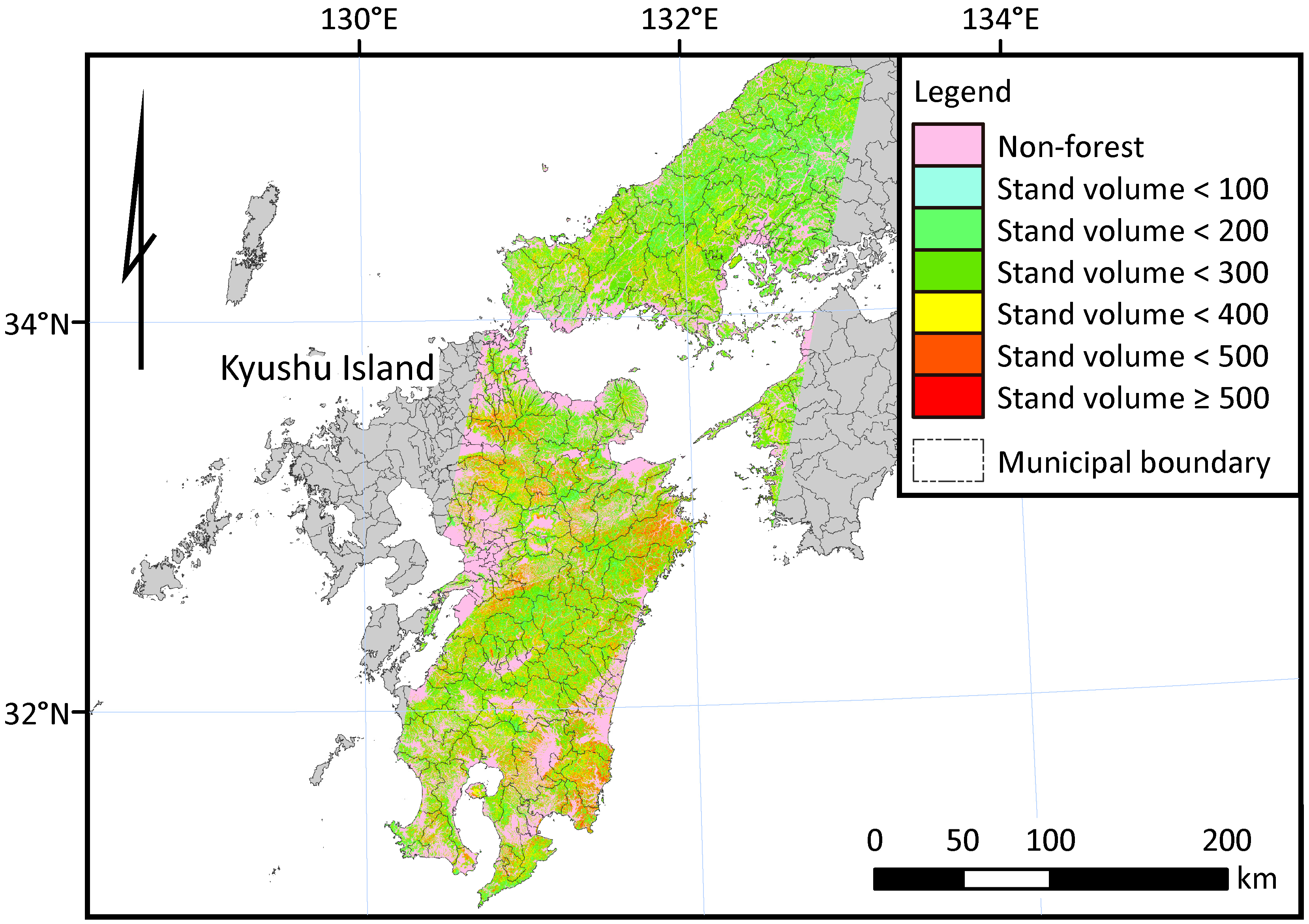
2.1. Study Area

A large area located in southwestern Japan, which covered all or part of nine prefectures (Ehime, Shimane, Hiroshima, Yamaguchi, Fukuoka, Oita, Kumamoto, Miyazaki and Kagoshima), was selected for the study (Figure 1). The study area included several tree species, such as Japanese cedar (Cryptomeria japonica), Japanese cypress (Chamaecyparis obtusa), Japanese red pine (Pinus densiflora), evergreen broad-leaved species (e.g., Quercus glauca, Castanopsis cuspidate and Machilus thunbergii) and deciduous broad-leaved species (e.g., Quercus serrata and Quercus acutissima). The climatic conditions differed significantly within the study area, because it extended more than 600 km in a latitudinal direction and encompassed a range of elevations exceeding 1700 m. Due to the climatic differences, the phenology of the vegetation within the study area varied considerably.

Figure 1. Location of the study area.

Figure 1. Location of the study area.

2.2. Satellite Image Data

Three sets of Landsat 7 ETM+ data acquired in three different seasons were used to estimate the stand volume (Table 1). The ETM+ data on three data tiles (three rows) between Row 36 and Row 38 on Path 112 of the World Reference System 2 (Figure 1) were downloaded via the Internet from the Earth Resources Observation and Science Center, United States Geological Survey. These data were acquired before the function of the scan line corrector built in the sensor of Landsat 7 failed. Because the thermal-infrared Band 6 has coarse spatial resolution (60 m), only visible, near-infrared and mid-infrared spectral bands (1–5 and 7) of ETM+ data, with a 30-m spatial resolution, were analyzed. The product types of all ETM+ data were Level 1T (standard terrain correction; L1T). The L1T products have been orthorectified using a DEM derived from the Shuttle Radar Topography Mission and resampled by the cubic convolution method.

Table 1. Information of the original ETM+ data used in this study.

Date	Sun Elevation Angle * (°)	Cloud Coverage ** (%)
4 April 2001	54.1	0
25 May 2002	65.7	0
12 July 2002	64.5	20.3

^* The average of Rows 36 to 38. The values of each scene were obtained from the scene header files. ^** The average of Rows 36 to 38. The cloud cover information was obtained from scene information provided by the USGS Global Visualization Viewer.

Table 1. Information of the original ETM+ data used in this study.

Date	Sun Elevation Angle * (°)	Cloud Coverage ** (%)
4 April 2001	54.1	0
25 May 2002	65.7	0
12 July 2002	64.5	20.3

^* The average of Rows 36 to 38. The values of each scene were obtained from the scene header files. ^** The average of Rows 36 to 38. The cloud cover information was obtained from scene information provided by the USGS Global Visualization Viewer.

We mosaicked ETM+ data tiles separately for each observation date. The mosaicked ETM+ data were re-registered to a mosaicked and orthorectified aerial photograph (acquired in about 1990; black-and-white; 1-m spatial resolution), because the ETM+ data had minor geometric errors. We employed the nearest-neighbor resampling method with a first-order polynomial equation with less than 0.5 pixels total RMSE. Following the geometric correction, we calculated the at-sensor spectral radiance from the digital numbers (DN) of the ETM+ data by the following equation:

$$L=\left(\frac{LMAX-LMIN}{Q_{\text{calmax}}-Q_{\text{calmin}}}\right)\times \left(Q_{\text{cal}}-Q_{\text{calmin}}\right)+LMIN$$

(1)

where L is the spectral radiance at the sensor’s aperture (W∙m⁻²∙sr⁻¹∙μm⁻¹), Q_cal is the quantized calibrated pixel value (DN), Q_calmin is the minimum quantized calibrated pixel value corresponding to LMIN, Q_calmax is the maximum quantized calibrated pixel value corresponding to LMAX, LMIN is the spectral at-sensor radiance that is scaled to Q_calmin (W∙m⁻²∙sr⁻¹∙μm⁻¹) and LMAX is the at-sensor spectral radiance scaled to Q_calmax (W∙m⁻²∙sr⁻¹∙μm⁻¹).

We did not perform any atmospheric correction via radiative transfer software due to the difficulty of ensuring a constant atmospheric condition under a single parameter setting for large areas. A dark object subtraction method [33,34] was used to make radiometric corrections to exclude path radiance, and then, a corrected radiance (L_cor) was obtained. Dark objects were selected from a single pixel in a clear water body via trial-and-error. Cloudy and hazy areas were visually identified and masked out manually. For the remaining areas, a constant atmospheric condition was assumed. In addition, we assumed that there were no atmospheric transmittance loss and no diffuse downward radiation at the surface and that the dark object in the remaining study area would remain absolutely dark, whereupon the reflectance (R) value was obtained from the L_cor with the following formula:

$$R=\frac{\pi \times L_{cor}\times d^2}{ESUN\times cos{\text{θ}}_s}$$

(2)

where π is a mathematical constant equal to ~3.14159 (unitless), d is the Earth-Sun distance (astronomical units), ESUN is the mean exoatmospheric solar irradiance (W∙m⁻²∙μm⁻¹) and θ_s is the solar zenith angle (degrees). In this study, the Earth-Sun distance values obtained from Chander et al. [35] were employed. This preprocessing is important, because most of the remote sensing applications are based on spectral reflectance; however, it should be noted that the standardization of DN would give the same results from spectral reflectance, since the processing of Equations (1) and (2) is a linear transformation (see Section 2.5). Because some previous studies reported that topographic normalization did not give clear results in k-NN estimation for satellite images with a high Sun elevation angle [36,37], we assumed there would be only minor topographic effects on the ETM+ data and did not perform topographic normalization in this study.

2.3. In Situ Data

We used plot-level stand volume data (m³/ha) derived from the first term of the FRMS as in situ data. The FRMS plots were set up at systematic 4-km grid intervals covering all forests in Japan. The first term of the FRMS was completed between April 1999, and March 2004. All plots are scheduled to be measured every five years, and about one-fifth of the plots are measured each year. Each plot is composed of three concentric circles with radii of 5.64 m (0.01 ha; S), 11.28 m (0.04 ha; M) and 17.84 m (0.10 ha; L), within which a total of 40 variables (nine for trees and understory vegetation and 31 for topography and other information) was measured by field crews. The size of trees to be measured was different for each circle; trees >1 cm, 5 cm and >18 cm in diameter at breast height (DBH) were measured in the S, M and L circles, respectively. In each plot, the tree height was measured for at least 20 trees, which were expected to be selected from a wide range of tree sizes to construct a DBH-height curve for the plot [23,25,31,38,39]. We used the information of species, DBH and tree height from the 40 measurement variables to calculate the plot-level stand volume. The individual stem volume was calculated from general two-way volume equations for each tree species; then, the summation of volume per 0.10 ha was defined as the observed stand volume in the field in this study.

During the first survey term, all FRMS plots were established by field crews with the help of Global Positioning System (GPS) navigation. According to the previous study [38], the location of FRMS plots had some positional errors. For example, some of the plots were subject to considerable positional errors (exceeding 20 m in RMSE). To avoid modeling errors due to positional inaccuracy between ETM+ data and field plot data, efforts to eliminate or to replace potentially erroneous data (e.g., sample plots falling near the forest/non-forest boundary) were employed in some previous studies [6,15,40,41,42]. In this study, we eliminated potentially erroneous data by the following steps: (1) we generated circular areas (radius of 50 m, corresponding to approximately 3 × 3 pixels of ETM+ data) based on the position coordinates of FRMS plots on the geographic information system (GIS) software; (2) the forest cover of the circular area was visually checked using the mosaicked aerial photograph and ETM+ data; (3) plots whose forest cover ratio for the circular area was less than 50% were eliminated; and (4) plots that were seemingly subject to dramatic changes by clear-cutting or other disturbance were excluded from the analysis [3,40]. In order to evaluate the accuracy of stand volume estimates appropriately for the three sets of Landsat 7 ETM+ data, we only selected the FRMS plots within cloudless areas on all ETM+ data. Consequently, a total of 891 FRMS plot data was used in this study.

2.4. Additional Feature Variables

As previously mentioned, we considered the use of forest type information for stand volume estimation. Because we did not have any accurate wall-to-wall digital maps of the forest types for this study area, we used forest type information (FTYPE; categorical variable), which was determined by the FRMS plot data itself. The FRMS plots were grouped into two classes (evergreen coniferous forest, ECF; broad-leaved forest, BF) by the dominant analysis [31,43] and the following procedures: (1) To obtain the dominant tree species group in all plots, first, all species of trees within each FRMS plot were classified into five tree species groups (evergreen coniferous, deciduous coniferous, evergreen broad-leaved, deciduous broad-leaved and bamboo); then, the dominant tree species group was determined based on the maximum basal area (m²) within each plot. (2) Plots that were dominated by bamboo trees were excluded from the analysis. Deciduous coniferous trees were not found in this study area, that is to say, the ECF class was only found for coniferous trees. (3) Two broad-leaved forest types (i.e., evergreen broad-leaved forest and deciduous broad-leaved forest) were aggregated and defined as BF, because of insufficient FRMS plots in these classes (for more detailed information on this procedure, see [31]). The sample sizes for the ECF and BF classes were 501 and 390, respectively. A summary of plot data concerning the stand volume is shown in Table 2.

Table 2. Summary of the plot stand volume data used in the present study following the removal of potentially erroneous data. ECF, evergreen coniferous forest; BF, broad-leaved forest.

Data	n	Mean (m3/ha)	SD (m3/ha)	Min (m3/ha)	Max (m3/ha)
All data	891	254.1	175.2	1.1	1,007.7
ECF	501	330.7	184.9	1.1	1,007.7
BF	390	155.7	95.1	2.5	665.0

Table 2. Summary of the plot stand volume data used in the present study following the removal of potentially erroneous data. ECF, evergreen coniferous forest; BF, broad-leaved forest.

Data	n	Mean (m3/ha)	SD (m3/ha)	Min (m3/ha)	Max (m3/ha)
All data	891	254.1	175.2	1.1	1,007.7
ECF	501	330.7	184.9	1.1	1,007.7
BF	390	155.7	95.1	2.5	665.0

A 10-m grid DEM derived from topographic maps at a 1:25,000 scale developed by photogrammetric interpretation, published by the Geospatial Information Authority of Japan, was used for the calculation of topographic-environmental factors. First, the grid size of the DEM was converted to 30 m by a bilinear interpolation resampling method; then, we computed the elevation (Elev), terrain slope angle (Slope), and solar radiation index (SRI [44]). We employed a 3 × 3 (i.e., 90 m × 90 m) moving window to calculate Slope in this study. Slope and SRI are calculated by the following formulae:

$$Slope={\tan }^{-1}\left(\frac{\sqrt{{(\mathrm{\Delta }x)}^2+{(\mathrm{\Delta }y)}^2}}{2}\right)\times \frac{180}{\text{π}}$$

(3)

where $\mathrm{\Delta }x$ and $\mathrm{\Delta }y$ are the average elevation changes per unit of distance in the x and y directions.

$$SRI=\cos (Lat)\cos (Slope)+\sin (Lat)\sin (Slope)\cos (Aspec{t}^{*})$$

(4)

where Lat is the latitude (degrees; north positive, south negative) and Aspect* is 180°-Aspect. Aspect was also computed by a 3 × 3 moving window.

The 1-km Mesh Climatic Data of Japan published by the Japan Meteorological Agency [45] was used for the calculation of climatic-environmental factors. We calculated Kira’s warmth index (WI) and coldness index (CI) [46], summer rainfall (SRF) (from June to September) and winter rainfall (WRF) (from November to February). The WI was calculated from the equation $\text{WI}={\displaystyle \sum }(\text{MT}-5)$, where the summation is made for the months in which the monthly mean temperature (MT) is higher than 5 °C, and the CI was calculated from the equation $\text{CI}=-{\displaystyle \sum }(5-\text{MT})$, where the summation is made for the winter months in which the MT is lower than 5 °C [47].

The mesh climatic data were calculated from meteorological observation data between 1971 and 2000 and interpolated with a 1-km mesh. Following computation, these four climatic-environmental factors were rasterized and converted from a grid size of 1 km to 30 m.

Although the use of explanatory variables that directly relate to the stand volume is very effective, it is extremely difficult to obtain such spatial data in wide ranges. Therefore, we used the above-mentioned seven environmental factors in the stand volume estimation.

2.5. Stand Volume Estimation and Accuracy Assessment

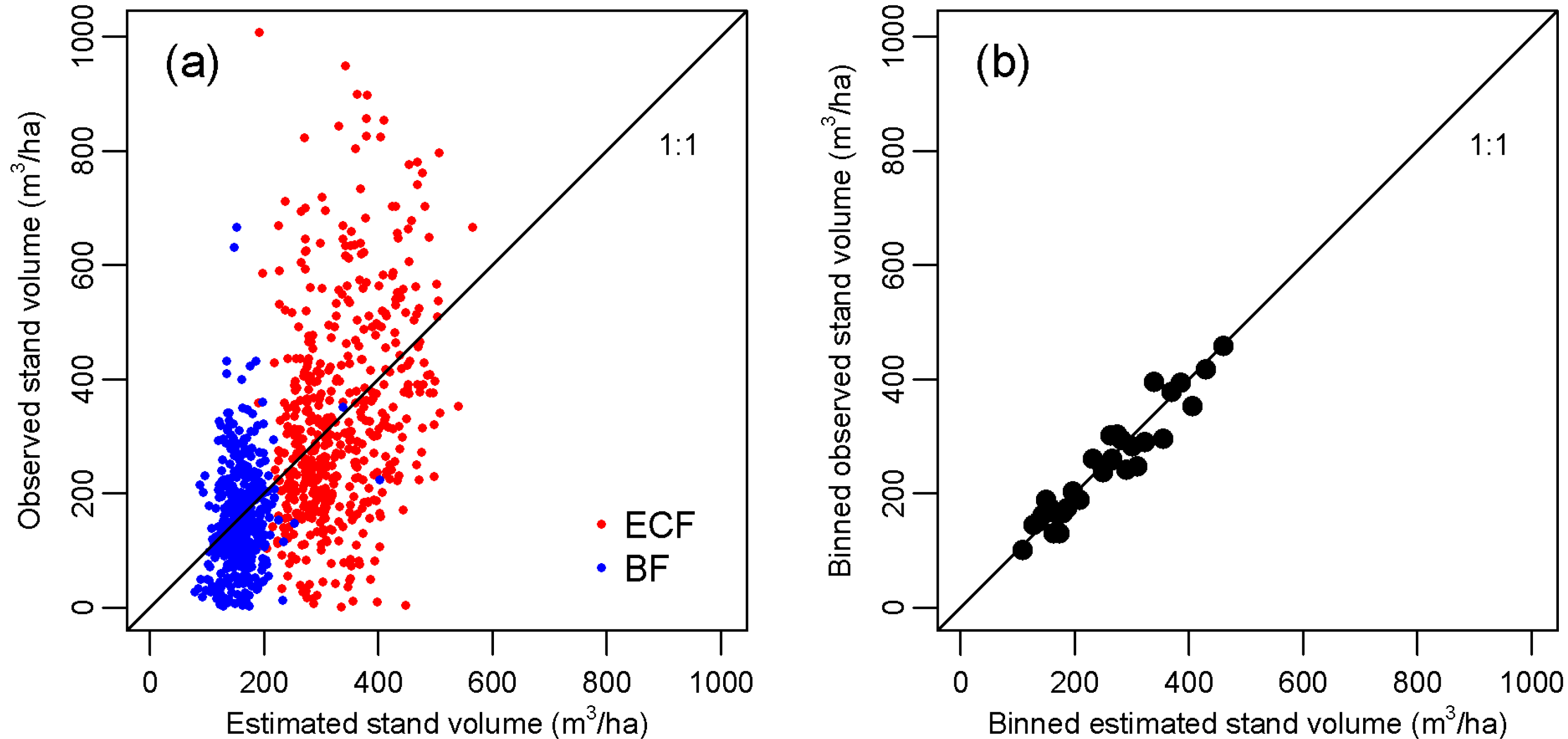
The reflectance data of six spectral bands (referred to simply as spectral data) on each seasonal ETM+ data, FTYPE and seven environmental factors were all stacked, and they are referred to as D0404, D0525 and D0712, respectively. Each dataset includes 14 variables (i.e., spectral data, FTYPE, Elev, Slope, SRI, WI, CI, SRF and WRF), and their ranges are different by each explanatory variable; so, all of the variables, except that of FTYPE, were standardized to avoid scale effects [21,48].

Using the k-NN technique, the stand volume can be estimated based on the simple assumption that the pixel to be estimated has a stand volume similar to the reference pixels. The stand volume for each pixel was calculated as the weighted mean stand volume of the reference pixel of the k-nearest samples in the feature space (explanatory variable space). The pixel weights, $w_{p_i,p}$, and estimates, ŷ_p, were calculated using the following equations:

$${\text{w}}_{p_i,p}=\frac{1}{d_{p_i,p}^t}/{\displaystyle \sum }_{j=1}^k\frac{1}{d_{p_j,p}^t}$$

(5)

$${\mathrm{ŷ}}_p={\displaystyle \sum }_{i=1}^k{w}_{p_i,p}\times y_{p_i}$$

(6)

where i is an arbitrary field plot, p is an arbitrary pixel, p_j is the pixel corresponding to the field plot j, d is the distance metric defined in the feature space, k is the number of reference plots, $y_{p_i}$ is the observed stand volume of the reference pixel $p_i$ and t ≥ 0 [14,49]. As the importance of each variable is different, some algorithms, such as k-MSN, PGNN and others, including the weighting of the distance metric [3,18], may be adequate when using different types of information. In addition, although fixed values of t = 0, 1 and 2 are usually used in the k-NN technique, the optimum value of t increases as k increases [49]. However, given its interpretive advantages [21] and the ease of comparing its results with those of previous studies [7,10,25,40,42,50,51,52], we used a simple k-NN technique with a fixed value of t = 2 in order to investigate the effectiveness of additional feature variables in this study.

First, we created prediction models without FTYPE and then created prediction models using FTYPE as a dummy variable. Hereafter, we define the former estimation as Analysis 1 and the latter as Analysis 2.

The selection of explanatory variables is a key procedure to remove uninformative or noisy variables for accurate stand volume estimation. We tested all possible variable combinations for the estimation of stand volume to find the best k-NN estimator (i.e., the optimum combination model). During this study, we examined the effectiveness of adding environmental factors to spectral data; therefore, the basic models (spectral data alone for Analysis 1, spectral data and FTYPE for Analysis 2) were fixed, and the variable selection was conducted only for the seven environmental factors. In each variable combination of each dataset and analysis, we selected the smallest value of k where the RMSE is not more than 1% greater than the smallest value of RMSE, as the optimum value of k [49,53].

We used the RMSE for accuracy assessment. To facilitate a comparison with previous studies (e.g., [7,10,25,40,42,50,51,52]), we also used relative RMSE (rRMSE, %). The RMSE and rRMSE were calculated using a leave-one-out cross-validation procedure with the following equations:

$$\text{RMSE}=\sqrt{\frac{1}{n}\times {\displaystyle \sum }_{i=1}^n{\left(y_i-{\mathrm{ŷ}}_i\right)}^2}$$

(7)

$$\text{rRMSE}=\frac{\sqrt{\frac{1}{n}\times {{\displaystyle \sum }}_{i=1}^n{\left(y_i-{\mathrm{ŷ}}_i\right)}^2}}{\overline{y}}\times 100$$

(8)

where y_i is the observed volume of the validation data i, ŷ_i is the estimated volume of i, n is the number of validation data and $\overline{y}$ is the mean of the observed stand volume. In accordance with McRoberts [49,54], another accuracy assessment was also performed graphically, taking the relationship between observed stand volume and estimated stand volume by a binned group of n = 30 samples by arranging estimated values in ascending order.

3. Results

Figure 2 shows the relationships between the RMSEs of the stand volume estimates and the number of explanatory variables used in Analysis 1. The results indicated that the addition of explanatory variables did not always contribute to error reduction. The numbers of additional feature variables used in the optimum combination models were one or three, suggesting that the relatively simple model performed well for stand volume estimation in our study area. The patterns of the relationships between the RMSEs of the stand volume estimates and the number of explanatory variables in Analysis 2 were the same as those in Analysis 1 (results are not shown).

Figure 2. Relationships between RMSEs of stand volume estimates and the number of explanatory variables for Analysis 1: (a) D0404; (b) D0525; (c) D0712. The RMSEs for six variables indicate the results from the basic models (spectral data alone), and the RMSEs for 13 variables indicate the results from all spectral data and environmental factors; the horizontal lines show the RMSEs of the estimates using basic models.

Figure 2. Relationships between RMSEs of stand volume estimates and the number of explanatory variables for Analysis 1: (a) D0404; (b) D0525; (c) D0712. The RMSEs for six variables indicate the results from the basic models (spectral data alone), and the RMSEs for 13 variables indicate the results from all spectral data and environmental factors; the horizontal lines show the RMSEs of the estimates using basic models.

When adding FTYPE to spectral data, the RMSE and the rRMSE of all datasets decreased (Table 3). The rRMSE of BF decreased from 73.9%–75.0% to 60.6%–62.7%, and the rRMSE of ECF decreased from 55.2%–56.7% to 53.2%–55.0%. The addition of FTYP had a greater positive effect on accuracy improvement for BF.

Table 3. Summary of RMSE and rRMSE for the stand volume estimates of the basic models for each dataset.

Error	D0404			D0525			D0712
	All	ECF	BF	All	ECF	BF	All	ECF	BF
Analysis 1
RMSE (m3/ha)	160.3	187.4	116.7	157.1	182.5	116.7	158.5	185.5	115.0
rRMSE (%)	63.1	56.7	75.0	61.8	55.2	75.0	62.4	56.1	73.9
Analysis 2
RMSE (m3/ha)	150.2	181.9	94.8	146.9	176.0	97.6	149.8	181.6	94.4
rRMSE (%)	59.1	55.0	60.9	57.8	53.2	62.7	59.0	54.9	60.6

Table 3. Summary of RMSE and rRMSE for the stand volume estimates of the basic models for each dataset.

Error	D0404			D0525			D0712
	All	ECF	BF	All	ECF	BF	All	ECF	BF
Analysis 1
RMSE (m3/ha)	160.3	187.4	116.7	157.1	182.5	116.7	158.5	185.5	115.0
rRMSE (%)	63.1	56.7	75.0	61.8	55.2	75.0	62.4	56.1	73.9
Analysis 2
RMSE (m3/ha)	150.2	181.9	94.8	146.9	176.0	97.6	149.8	181.6	94.4
rRMSE (%)	59.1	55.0	60.9	57.8	53.2	62.7	59.0	54.9	60.6

The RMSEs of the estimates decreased with the addition of some variables, but increased with the addition of others (Table 4). For example, the addition of most environmental factors to the spectral data effectively improved the accuracy of D0404 and D0712, and the addition of most environmental factors negatively affected D0525. The addition of one specific environmental factor to the basic models revealed that the addition of SRF had a consistent positive effect on accuracy improvement. In Analysis 1, the addition of SRF reduced the RMSE by 2.5, 2.0 and 1.5 m³/ha for D0404, D0525 and D0712, respectively. Similarly, in Analysis 2, the addition of SRF reduced the RMSE by 2.3, 0.7 and 1.6 m³/ha for D0404, D0525 and D0712, respectively. Although there were some exceptions (especially for D0525), WI and CI had positive effects on accuracy improvement. In contrast, Slope and SRI negatively affected the stand volume estimation in most cases.

Table 4. RMSE (m³/ha) of each variable combination in each dataset and analysis. Elev, elevation; SRI, solar radiation index; WI, warmth index; CI, coldness index; SRF, summer rainfall; WRF, winter rainfall.

Model	Analysis 1			Analysis 2
	D0404	D0525	D0712	D0404	D0525	D0712
Basic model	160.3	157.1	158.5	150.2	146.9	149.8
Basic model + Elev	159.1	157.9	158.0	149.4	148.7	148.9
Basic model + Slope	160.6	159.0	158.6	151.5	148.6	150.2
Basic model + SRI	161.8	158.3	159.3	152.1	148.2	149.8
Basic model + WI	159.9	157.4	157.8	149.5	147.4	148.7
Basic model + CI	159.7	157.4	157.0	148.8	147.6	148.1
Basic model + SRF	157.8	155.2	157.0	147.9	146.2	148.3
Basic model + WRF	160.3	156.8	158.3	150.7	146.5	149.3
Optimum combination model	157.8 a	155.2 b	155.1 c	147.2 d	146.2 e	145.8 f

Values with an underline indicate cases where the RMSE was reduced compared with basic models. Explanatory variables of optimum combination models are: ^a spectral data and SRF; ^b spectral data and SRF; ^c spectral data, Elev, WI and SRF; ^d spectral data, FTYPE (forest type information), CI and SRF; ^e spectral data, FTYPE and SRF; ^f spectral data, FTYPE, CI and SRF.

Table 4. RMSE (m³/ha) of each variable combination in each dataset and analysis. Elev, elevation; SRI, solar radiation index; WI, warmth index; CI, coldness index; SRF, summer rainfall; WRF, winter rainfall.

Model	Analysis 1			Analysis 2
	D0404	D0525	D0712	D0404	D0525	D0712
Basic model	160.3	157.1	158.5	150.2	146.9	149.8
Basic model + Elev	159.1	157.9	158.0	149.4	148.7	148.9
Basic model + Slope	160.6	159.0	158.6	151.5	148.6	150.2
Basic model + SRI	161.8	158.3	159.3	152.1	148.2	149.8
Basic model + WI	159.9	157.4	157.8	149.5	147.4	148.7
Basic model + CI	159.7	157.4	157.0	148.8	147.6	148.1
Basic model + SRF	157.8	155.2	157.0	147.9	146.2	148.3
Basic model + WRF	160.3	156.8	158.3	150.7	146.5	149.3
Optimum combination model	157.8 a	155.2 b	155.1 c	147.2 d	146.2 e	145.8 f

Values with an underline indicate cases where the RMSE was reduced compared with basic models. Explanatory variables of optimum combination models are: ^a spectral data and SRF; ^b spectral data and SRF; ^c spectral data, Elev, WI and SRF; ^d spectral data, FTYPE (forest type information), CI and SRF; ^e spectral data, FTYPE and SRF; ^f spectral data, FTYPE, CI and SRF.

Figure 3 shows the estimated stand volume from the optimum combination model of D0525 in Analysis 2. The estimated stand volume was overestimated for smaller volumes and underestimated for larger volumes (Figure 3a). However, the graph of the binned observations versus the binned estimates revealed that there was no bias in the results (Figure 3b). Similarly, all of the other models that included the basic models of Analysis 1 showed no biases in the results (results not shown).

Figure 3. Scatter plot of the observed stand volume versus the estimated stand volume using the optimum combination model of D0525 in Analysis 2. (a) Pixel-level observed stand volume versus estimated stand volume. (b) Binned pixel-level observed stand volume versus binned pixel-level estimated stand volume (group size = 30). The explanatory variables of the optimum combination model of D0525 were spectral data, FTYPE and SRF. The optimum value of k = 20 (the smallest value of k for which the RMSE was not greater than 1% of the smallest RMSE value) was used.

Figure 3. Scatter plot of the observed stand volume versus the estimated stand volume using the optimum combination model of D0525 in Analysis 2. (a) Pixel-level observed stand volume versus estimated stand volume. (b) Binned pixel-level observed stand volume versus binned pixel-level estimated stand volume (group size = 30). The explanatory variables of the optimum combination model of D0525 were spectral data, FTYPE and SRF. The optimum value of k = 20 (the smallest value of k for which the RMSE was not greater than 1% of the smallest RMSE value) was used.

Finally, we created a spatial distribution map of stand volume in the study area. Figure 4 shows a map of stand volume estimated by the optimum combination model for D0525 from Analysis 1. This map clearly shows the differences in stand volume among municipal units, as well as the differences in stand volume within a municipal unit. The map shows that there are many “hot spots” of high stand volume values (displayed with orange and red colors) in Kyushu Island (e.g., stand volume ≥ 400 m³/ha), and the northern region of the study area shows relatively low stand volume.

4. Discussion

When we used spectral data alone, the rRMSEs of the estimates ranged from 62.0% to 63.2% in Analysis 1 and from 58.2% to 59.9% in Analysis 2, respectively (Table 3). Although the RMSEs of our results at the pixel level were larger than those reported by some previous studies, they were moderate compared with those reported by previous studies, e.g., 44.2% (China [7]), 47.6% (Finland [50]), 58%–80% (Sweden [42]), 59.0% (Sweden [52]), 66.2% (Japan [25]), 66.6% (Sweden [40]), 79.3% (Finland [51]) and 91% (Norway [10]). Accordingly, the stand volume in Japan could be estimated by the k-NN technique with accuracies similar to earlier studies in terms of the rRMSE.

Figure 4. Map of the estimated stand volume. Estimates made by the optimum combination model of D0525 from Analysis 1 are shown as an example. The explanatory variables of the model were spectral data and SRF. The optimum value of k = 21 was used. Non-forest mask was generated from GIS data (“National Land numerical information (Forest Region Version 3.1), Ministry of Land, Infrastructure, Transport and Tourism”).

Figure 4. Map of the estimated stand volume. Estimates made by the optimum combination model of D0525 from Analysis 1 are shown as an example. The explanatory variables of the model were spectral data and SRF. The optimum value of k = 21 was used. Non-forest mask was generated from GIS data (“National Land numerical information (Forest Region Version 3.1), Ministry of Land, Infrastructure, Transport and Tourism”).

There are many reasons for the large RMSEs of pixel-level results, including outliers due to the spatial mismatch between the satellite image pixels and the field plots, within the scene variation of the atmospheric effect, and so on [3,49]. In particular, the high value and wide range of stand volume of the ECF class of Japanese forests is one of the main reasons for large RMSEs [25], because the pattern of small-value overestimation and high-value underestimation (Figure 3a) is typical for the k-NN technique [21,25,40,42]. Moreover, if we did not remove the FRMS plot data falling near the forest/non-forest boundary in this study, the RMSEs of the estimates might have been much larger.

When we used the combination models in addition to the basic models, the RMSEs of the estimates decreased for some variable combinations and increased for others (Figure 2 and Table 4). In other words, the positive effects of the environmental factors were not always as expected. As the inclusion of unrelated variables used to calculate distances would cause detrimental effects on accuracy [49,53], careful variable selection should be performed to avoid negative effects on estimation accuracy when using environmental factors as explanatory variables in the k-NN technique.

Compared with the six other environmental factors, SRF had a consistent positive effect on error reduction (Table 4). This consistency is important to apply this approach to operational tasks, such as the creation of nationwide stand volume maps. The combination of spectral data with SRF may be useful to estimate stand volume more accurately than in the case of spectral data alone. Compared with topographic-environmental factors, such as Slope and SRI, climatic-environmental factors, such as SRF, have a more significant spatial autocorrelation. Therefore, when adding SRF to the basic model, the nearest neighbors are selected from geographically closer plots. A previous study in Finland reported that the consideration of the geographic distance of nearest neighbor plots was useful for stand volume estimation, because of the gradual changes in vegetation structure in satellite images [17]. Therefore, we assumed that the plots geographically close to the target pixel tend to be selected as nearest neighbors using SRF, and this may lead to improvements in the accuracy of stand volume estimations; however, this approach is different from that used by Katila and Tomppo [17].

Meanwhile, the positive effects of the addition of FTYPE were obvious in cases of both the spectral data alone (RMSE reduced by 8.7–10.2 m³/ha) and the optimum combination model (RMSE reduced by 8.9–10.7 m³/ha) (Table 4). The accuracy improvement was large for the BF class, because the predictive ability of the models derived from the spectral data alone was insufficient (rRMSE ranging 73.9%–75.0%, Table 3). When adopting the k-NN technique in Japan and other countries with both coniferous and broad-leaved forests similar to our study area, the use of FTYPE would be useful for mapping stand volume more accurately.

As shown in Figure 4, there are clear differences in stand volume estimates among municipal units. Although the stand volume estimates made in this study showed overestimations for smaller volumes and underestimations for larger volumes, the binned assessment showed that there was no bias in the estimations made with the k-NN technique (Figure 3), as there was in some previous studies [49,54]. The accuracy of estimates is improved when the aggregated pixels are evaluated [3,21]. Therefore, although the pixel-level estimates made using the k-NN technique presented here have insufficient accuracy for forestry operations, they are useful for assessing the total or average stand volume at regional and national scales for strategic forest planning.

In this study, we used FTYPE, which was determined by the field plot data itself; however, in order to estimate stand volume accurately for unknown pixels, it is necessary to use additional digital maps concerning the forest type for the whole area being analyzed. Therefore, to efficiently use the method presented in this study, an accurate forest type map must be prepared, either manually or via an automatic image classification of remotely-sensed data.

The mapping of forest type is an ongoing project [55]. Additional investigations should be conducted on mapping stand volumes and their uncertainties when using wall-to-wall digital forest type maps in accordance with some previous studies [21,22]. These analyses and map products are expected to improve forest statistics at the regional and national scale and to support sustainable forest management in Japan.

5. Conclusions

To evaluate the effectiveness of adding feature variables to satellite image data on the accuracy of stand volume estimates using the k-NN technique, the estimates from three Landsat ETM+ datasets acquired in different seasons with various combinations of additional feature variables were compared.

The results showed that the addition of environmental factors to satellite image data did not always help to improve estimation accuracy. To avoid negative effects on the accuracy of stand volume estimates, careful variable selection should be performed. Among the environmental factors tested in this study, summer rainfall data had a consistent positive effect on accuracy improvement. Therefore, summer rainfall data may be a useful feature variable in stand volume estimations in this study area. The use of forest type information improved the estimation accuracy, particularly for broad-leaved forests. When adopting the k-NN technique in Japan and other countries with both coniferous and broad-leaved forests similar to our study area, the use of forest type information would be useful for mapping stand volume accurately. The binned assessment of stand volume estimates showed that there were no biases in the estimations made with the k-NN technique. Thus, such a map of estimated stand volume would be useful for assessing the total or average stand volume at regional and national scales for strategic forest planning.

All of these results indicated that the k-NN technique combined with appropriate feature variables is applicable to nationwide stand volume estimation in Japan. To ensure our results and to accurately estimate the stand volume for unknown pixels, additional investigations should be conducted on mapping stand volumes and their uncertainties when using wall-to-wall digital forest type maps. In the same manner, the effectiveness of summer rainfall data should be tested in other regions where the climatic characteristics differ from those of our study area.

References

1. Tomppo, E.; Schadauer, K.; McRoberts, R.E.; Gschwantner, T.; Gabler, K.; Ståhl, G. Introduction. In National Forest Inventories: Pathways for Common Reporting; Tomppo, E., Gschwantner, Th., Lawrence, M., McRoberts, R.E., Eds.; Springer-Verlag: New York, NY, USA, 2010; pp. 1–18. [Google Scholar]
2. Tomppo, E.; Haakana, M.; Katila, M.; Peräsaari, J. Multi-Source National Forest Inventory: Methods and Applications; Springer: New York, NY, USA, 2008. [Google Scholar]
3. Tomppo, E.; Olsson, H.; Ståhl, G.; Nilsson, M.; Hagner, O.; Katila, M. Combining national forest inventory field plots and remote sensing data for forest databases. Remote Sens. Environ. 2008, 112, 1982–1999. [Google Scholar] [CrossRef]
4. Olsson, H.; Nilsson, M.; Persson, A. GEOSS possibilities and challenges related to nation wide forest monitoring. In Proceedings of the ISPRS Commission VII Term Symposium, Enschede, The Netherlands, 8–11 May 2006.
5. McRoberts, R.E.; Tomppo, E.O. Remote sensing support for national forest inventories. Remote Sens. Environ. 2007, 110, 412–419. [Google Scholar] [CrossRef]
6. Reese, H.; Nilsson, M.; Granqvist Pahlén, T.; Hagner, O.; Joyce, S.; Tingelöf, U.; Egberth, M.; Olsson, H. Countrywide estimates of forest variables using satellite data and field data from the National Forest Inventory. Ambio 2003, 32, 542–548. [Google Scholar] [PubMed]
7. Gu, H.; Dai, L.; Wu, G.; Xu, D.; Wang, S.; Wang, H. Estimation of forest volumes by integrating Landsat TM imagery and forest inventory data. Sci. China Ser. E Technol. Sci. 2006, 49, 54–62. [Google Scholar] [CrossRef]
8. Tomppo, E.; Korhonen, K.T.; Heikkinen, J.; Yli-Kojola, H. Multi-source inventory of the forests of the Hebei forestry bureau, Heilongjiang, China. Silva Fenn. 2001, 35, 309–328. [Google Scholar] [CrossRef]
9. McInerney, D.O.; Nieuwenhuis, M. A comparative analysis of kNN and decision tree methods for the Irish National Forest Inventory. Int. J. Remote Sens. 2009, 30, 4937–4955. [Google Scholar] [CrossRef]
10. Gjertsen, A.K. Accuracy of forest mapping based on Landsat TM data and a kNN-based method. Remote Sens. Environ. 2007, 110, 420–430. [Google Scholar] [CrossRef]
11. McRoberts, R.E.; Holden, G.R.; Nelson, M.D.; Liknes, G.C.; Gormanson, D.D. Using satellite imagery as ancillary data for increasing the precision of estimates for the Forest Inventory and analysis program of the USDA Forest Service. Can. J. For. Res. 2006, 36, 2968–2980. [Google Scholar]
12. Nilsson, M.; Folving, S.; Kennedy, P.; Puumalainen, J.; Chirici, G.; Corona, P.; Marchetti, M.; Olsson, H.; Ricotta, C.; Ringvall, A.; et al. Combining remote sensing and field data for deriving unbiased estimated of forest parameters over large regions. In Advances in Forest Inventory for Sustainable Forest Management and Biodiversity Monitoring; Corona, P., KöhlKöhl, M., Marchetti, M., Eds.; Kruwer Academic Publishers: Dordrecht, The Netherlands, 2003; pp. 19–32. [Google Scholar]
13. Nilsson, M.; Holm, S.; Reese, H.; Wallerman, J.; Engberg, J. Improved forest statistics from the Swedish National Inventory by combining field data and optical satellite data using post-stratification. In Proceedings of the ForestSat 2005, Borȧs, Sweden, 31 May–3 June 2005.
14. Tomppo, E. Multi-source national forest inventory of Finland. In Proceedings of the IUFRO XX World Congress, Tampere, Finland, 6–12 August 1995; Paivinen, R., Vanclay, J., Miina, S., Eds.; EFI: Joensuu, Finland, 1996; pp. 27–41. [Google Scholar]
15. Tokola, T.; Heikkilä, J. Improving satellite image based forest inventory by using a priori site quality information. Silva Fenn. 1997, 31, 67–78. [Google Scholar] [CrossRef]
16. Tomppo, E.; Goulding, C.; Katila, M. Adapting finnish multi-source forest inventory techniques to the New Zealand preharvest inventory. Scand. J. For. Res. 1999, 14, 182–192. [Google Scholar] [CrossRef]
17. Katila, M.; Tomppo, E. Selecting estimation parameters for the Finnish multisource National Forest Inventory. Remote Sens. Environ. 2001, 76, 16–32. [Google Scholar] [CrossRef]
18. Tomppo, E.; Halme, M. Using coarse scale forest variables as ancillary information and weighting of variables in k-NN estimation: A genetic algorithm approach. Remote Sens. Environ. 2004, 92, 1–20. [Google Scholar] [CrossRef]
19. Moeur, M.; Stage, A.R. Most similar neighbor: An improved sampling inference procedure for natural resource planning. For. Sci. 1995, 41, 337–359. [Google Scholar]
20. Packalén, P.; Maltamo, M. The k-MSN method for the prediction of species-specific stand attributes using airborne laser scanning and aerial photographs. Remote Sens. Environ. 2007, 109, 328–341. [Google Scholar] [CrossRef]
21. Beaudoin, A.; Bernier, P.Y.; Guindon, L.; Villemaire, P.; Guo, X.J.; Stinson, G.; Bergeron, T.; Magnussen, S.; Hall, R.J. Mapping attributes of Canada’s forests at moderate resolution through kNN and MODIS imagery. Can. J. For. Res. 2014, 44, 521–532. [Google Scholar] [CrossRef]
22. Wilson, B.T.; Woodall, C.W.; Griffith, D.M. Imputing forest carbon stock estimates from inventory plots to a nationally continuous coverage. Carbon Balance Manag. 2013, 8, 1–15. [Google Scholar] [CrossRef] [PubMed]
23. Hirata, Y.; Imaizumi, Y.; Masuyama, T.; Matsumoto, Y.; Miyazono, H.; Goto, T. Japan. In National Forest Inventories: Pathways for Common Reporting; Tomppo, E., Gschwantner, Th., Lawrence, M., McRoberts, R.E., Eds.; Springer-Verlag: New York, NY, USA, 2010; pp. 333–340. [Google Scholar]
24. Iehara, T. New Japanese forest resource monitoring system. Sanrin 1999, 1384, 54–61. [Google Scholar]
25. Kajisa, T.; Murakami, T.; Mizoue, N.; Kitahara, F.; Yoshida, S. Estimation of stand volumes using the k-nearest neighbors method in Kyushu, Japan. J. For. Res. 2008, 13, 249–254. [Google Scholar] [CrossRef]
26. Minowa, Y.; Suzuki, N.; Tanaka, K. Estimation of site indices with a machine learning system C4.5. Jpn. J. For. Plan. 2005, 38, 143–156. [Google Scholar]
27. Minowa, Y.; Suzuki, N.; Tanaka, K. Estimation of site indices with an artificial neural network. Jpn. J. For. Plan. 2005, 39, 23–38. [Google Scholar]
28. Mitsuda, Y.; Yoshida, S.; Imada, M. Use of GIS-derived environmental factors in predicting site indices in Japanese larch plantations in Hokkaido. J. For. Res. 2001, 6, 87–93. [Google Scholar] [CrossRef]
29. Mitsuda, Y.; Ito, S.; Sakamoto, S. Predicting the site index of sugi plantations from GIS-derived environmental factors in Miyazaki Prefecture. J. For. Res. 2007, 12, 177–186. [Google Scholar] [CrossRef]
30. Nabeshima, E.; Kubo, T.; Hiura, T. Variation in tree diameter growth in response to the weather conditions and tree size in deciduous broad-leaved trees. For. Ecol. Manag. 2010, 259, 1055–1066. [Google Scholar] [CrossRef]
31. Nishizono, T.; Kitahara, F.; Iehara, T.; Mitsuda, Y. Geographical variation in age—Height relationships for dominant trees in Japanese cedar (Cryptomeria japonica D. Don) forests in Japan. J. For. Res. 2014, 19, 305–316. [Google Scholar] [CrossRef]
32. Teraoka, Y.; Masutani, T.; Imada, M. Estimating site index of Sugi and Hinoki from topographical factors on maps for forest management. Sci. Bull. Fac. Agric. Kyushu Univ. 1991, 45, 125–133. [Google Scholar]
33. Chavez, P.S., Jr. An improved dark-object subtraction technique for atmospheric scattering correction of multispectral data. Remote Sens. Environ. 1988, 24, 459–479. [Google Scholar] [CrossRef]
34. Teillet, P.M.; Fedosejevs, G. On the dark target approach to atmospheric correction of remotely sensed data. Can. J. Remote Sens. 1995, 24, 374–387. [Google Scholar] [CrossRef]
35. Chander, G.; Markham, B.L.; Helder, D.L. Summary of current radiometric calibration coefficients for Landsat MSS, TM, ETM+, and EO-1 ALI sensors. Remote Sens. Environ. 2009, 113, 893–903. [Google Scholar] [CrossRef]
36. Chirici, G.; Barbati, A.; Corona, P.; Marchetti, M.; Travaglini, D.; Maselli, F.; Bertini, R. Non-parametric and parametric methods using satellite images for estimating growing stock volume in alpine and Mediterranean forest ecosystems. Remote Sens. Environ. 2008, 112, 2686–2700. [Google Scholar] [CrossRef] [Green Version]
37. Tanaka, S.; Takahashi, T.; Saito, H.; Nishizono, T.; Iehara, T.; Kitahara, F.; Kodani, E.; Awaya, Y. Stand volume estimation using Landsat ETM+ data through atmospheric and topographic corrections in the Tohoku region, Japan. Jpn. J. For. Plan. 2013, 47, 29–34. [Google Scholar]
38. Kitahara, F.; Mizoue, N.; Kajisa, T.; Yoshida, S. Positional accuracy of national forest inventory plots in Japan. J. For. Plan. 2010, 15, 73–79. [Google Scholar]
39. Kitahara, F.; Mizoue, N.; Yoshida, S. Evaluation of data quality in Japanese National Forest Inventory. Environ. Monit. Assess. 2009, 159, 331–340. [Google Scholar] [CrossRef] [PubMed]
40. Fazakas, Z.; Nilsson, M.; Olsson, H. Regional forest biomass and wood volume estimation using satellite data and ancillary data. Agric. For. Meteorol. 1999, 98–99, 417–425. [Google Scholar] [CrossRef]
41. Hagner, O.; Reese, H. A method for calibrated maximum likelihood classification of forest types. Remote Sens. Environ. 2007, 110, 438–444. [Google Scholar] [CrossRef]
42. Reese, H.; Nilsson, M.; Sandström, P.; Olsson, H. Applications using estimates of forest parameters derived from satellite and forest inventory data. Comput. Electron. Agric. 2002, 37, 37–55. [Google Scholar] [CrossRef]
43. Ohsawa, M. Differentiation of vegetation zones and species strategies in the subalpine region of Mt. Fuji. Vegetatio 1984, 57, 15–52. [Google Scholar] [CrossRef]
44. Keating, K.A.; Gogan, P.J.P.; Vore, J.M.; Irby, L.R. A simple solar radiation index for wildlife habitat studies. J. Wildl. Manag. 2007, 71, 1344–1348. [Google Scholar] [CrossRef]
45. Japan Meteorological Agency. Mesh Climatic Data of Japan (CD-ROM); Japan Meteorological Business Support Center: Tokyo, Japan, 2002. [Google Scholar]
46. Kira, T. A New Classification of Climate in Eastern Asia as the Basis for Agricultural Geography; Horicultural Institute, Kyoto University: Kyoto, Japan, 1945; pp. 1–23. [Google Scholar]
47. Kira, T. Forest ecosystems of east and southeast Asia in a global perspective. Ecol. Res. 1991, 6, 185–200. [Google Scholar] [CrossRef]
48. LeMay, V.; Temesgen, H. Comparison of nearest neighbor methods for estimating basal area and stems per hectare using aerial auxiliary variables. For. Sci. 2005, 51, 109–119. [Google Scholar]
49. McRoberts, R.E. Estimating forest attribute parameters for small areas using nearest neighbors techniques. For. Ecol. Manag. 2012, 272, 3–12. [Google Scholar] [CrossRef]
50. Mäkelä, H.; Pekkarinen, A. Estimation of timber volume at the sample plot level by means of image segmentation and Landsat TM imagery. Remote Sens. Environ. 2001, 77, 66–75. [Google Scholar] [CrossRef]
51. Mäkelä, H.; Pekkarinen, A. Estimation of forest stand volumes by Landsat TM imagery and stand-level field-inventory data. For. Ecol. Manag. 2004, 196, 245–255. [Google Scholar] [CrossRef]
52. Tomppo, E.; Nilsson, M.; Rosengren, M.; Aalto, P.; Kennedy, P. Simultaneous use of Landsat-TM and IRS-1C WiFS data in estimating large area tree stem volume and aboveground biomass. Remote Sens. Environ. 2002, 82, 156–171. [Google Scholar] [CrossRef]
53. McRoberts, R.E.; Nelson, M.D.; Wendt, D.G. Stratified estimation of forest area using satellite imagery, inventory data, and the k-Nearest Neighbors technique. Remote Sens. Environ. 2002, 82, 457–468. [Google Scholar] [CrossRef]
54. McRoberts, R.E. Diagnostic tools for nearest neighbors techniques when used with satellite imagery. Remote Sens. Environ. 2009, 113, 489–499. [Google Scholar] [CrossRef]
55. Tanaka, S.; Takahashi, T.; Saito, H.; Awaya, Y.; Iehara, T.; Matsumoto, M.; Sakai, T. Simple method for land-cover mapping by combining multi-temporal Landsat ETM+ images and systematically sampled ground truth data: A case study in Japan. J. For. Plan. 2012, 18, 77–85. [Google Scholar]