Estimating Forest Biomass Dynamics by Integrating Multi-Temporal Landsat Satellite Images with Ground and Airborne LiDAR Data in the Coal Valley Mine, Alberta, Canada

Abstract

Assessing biomass dynamics is highly critical for monitoring ecosystem balance and its response to climate change and anthropogenic activities. In this study, we introduced a direct link between Landsat vegetation spectral indices and ground/airborne LiDAR data; this integration was established to estimate the biomass dynamics over various years using multi-temporal Landsat satellite images. Our case study is located in an area highly affected by coal mining activity. The normalized difference vegetation index (NDVI), enhanced vegetation index (EVI and EVI2), chlorophyll vegetation index (CVI), and tasseled cap transformations were used as vegetation spectral indices to estimate canopy height. In turn, canopy height was used to predict a coniferous forest’s biomass using Jenkins allometric and Lambert and Ung allometric equations. The biophysical properties of 700 individual trees at eight different scan stations in the study area were obtained using high-resolution ground LiDAR. Nine models (H_i) were established to discover the best relationship between the canopy height model (CHM) from the airborne LiDAR and the vegetation spectral indices (VSIs) from Landsat images for the year 2005, and HB₉ (Jenkins allometric equation) and HY₉ (Lambert and Ung allometric equation) proved to be the best models (r² = 0.78; root mean square error (RMSE) = 44 Mg/H, r² = 0.67; RMSE = 58.01 Mg/H, respectively; p < 0.001) for estimating the canopy height and the biomass. This model accurately captured the most affected areas (deforested) and the reclaimed areas (forested) in the study area. Five years were chosen for studying the biomass change: 1988, 1990, 2001, 2005, and 2011. Additionally, four pixel-based image comparisons were analyzed (i.e., 1988–1990, 1990–2005, 2005–2009, and 2009–2011), and Mann-Kendall statistics for the subsets of years were obtained. The detected change showed that, in general, the environment in the study area was recovering and regaining its initial biomass after the dramatic decrease that occurred in 2005 as a result of intensive mining activities and disturbance.

1. Introduction

Monitoring forest biomass dynamics is known as one of the important factors for environmental modeling [1], and obtaining information on forest biomass dynamics has become a necessity for forest management [2]. Additionally, improving the monitoring techniques to assess forest biomass change is required to understand anthropogenic effects on ecosystem balance [3].

In the last decade, the use of passive and active remote sensing sensors to monitor forest biomass has received attention due to their ability to model the carbon cycle, deforestation and forest degradation [4,5,6]. The recent advances in ground and airborne light detection and ranging (LiDAR) remote sensing enable more accurate data acquisition for the vertical and horizontal vegetation structure and better estimation of forest biomass [7,8]. Many investigations have used LiDAR data to estimate biomass by considering the statistical relationship between field measurements and airborne LiDAR [7,9,10]. Data from high-resolution ground LiDAR will maximize accuracy and minimize uncertainty in the findings [11,12,13]. The main purpose of using LiDAR data in our investigation is to measure the biophysical parameters of trees, such as the diameter at breast height (DBH), tree height and canopy width. Multi-spectral optical remote sensing, such as Landsat Thematic Mapper (TM) satellite images, is a valuable data source in ecological research for estimating multi-temporal biomass dynamics and has been widely used for monitoring vegetation cover [14,15,16,17]. Also, Pflugmacher et al. [3] discussed the limitations of estimating biomass using multi-spectral sensors, namely, the misrepresentation of the actual spatial distribution of the biomass. Additionally, the difficulty of evaluating the sampling errors because of the spatial resolution heterogeneity between remote sensing data, field surveys, and biomass maps has been discussed by [18,19]. Many scientists succeeded in enhancing the relationship between Landsat spectral indices and forest biomass by incorporating the spectral trajectory of forest disturbance and regrowth, which decreased the root mean square error (RMSE) from 57% to 41% [20].

The allometric equations are useful for estimating biomass in North America, and were collected from different research papers for various tree species [21,22,23]. Equations that are suitable for a large number of species have been developed [24,25] to correct the allometric equations previously published, such as in [26,27,28,29]. Additionally, many scientists have adopted various allometric equations in their case studies because they can be used to address the spatial variability [28,30,31].

Our case study involves a mining area in the western central area of the province of Alberta in Canada, where huge areas were affected by deforestation as a result of coal mining activities. Such anthropological activity introduce abiotic chemical and physical disturbance such as pH (soil acidity and alkalinity), soil salinity, soil compaction, and low hydraulic conductivity, and these factors harm the soil fertility and the ecosystem balance and cause degradations over time [32,33,34].

The main objective of this investigation is to obtain the multi-spatiotemporal biomass distribution from optical remote sensing data for a coniferous forest on a coal mining site. To achieve this goal, we first addressed several research challenges:

(a)

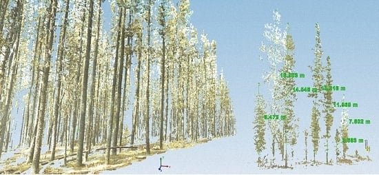
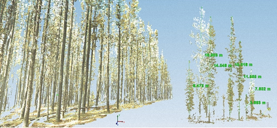
Using high-resolution ground LiDAR to find the relationship between different biophysical parameters, including tree height, DBH and canopy width,

(b)

Applying a ground-LiDAR-based regression model to two allometric equations to estimate the biomass values from the CHM of the airborne LiDAR,

(c)

Finding the best spectral-based regression model to predict the coniferous forest biomass from multi-temporal Landsat data, and

(d)

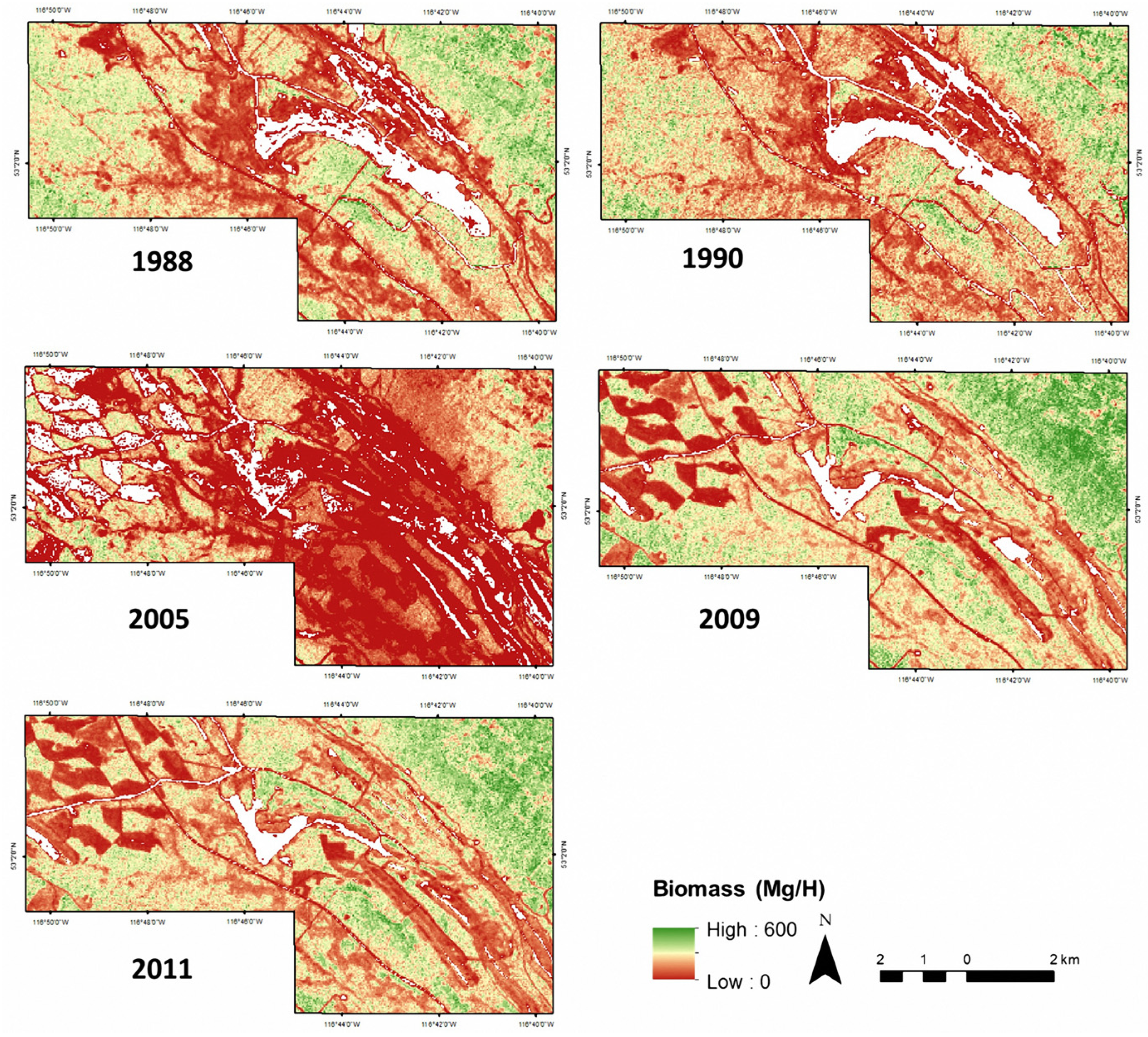
Assessing the change in the biomass in 1988, 1990, 2001, 2005, and 2011.

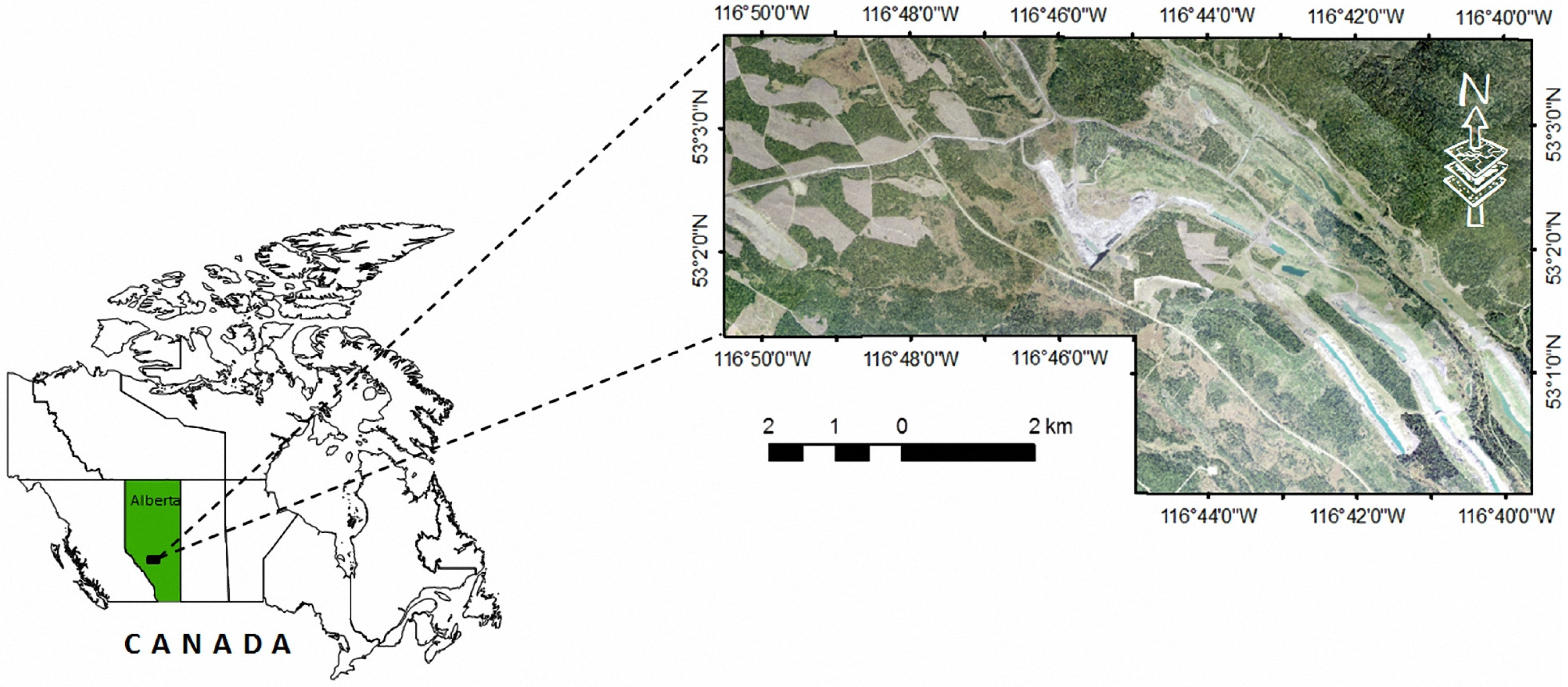
2. Case Study Description

The case study was conducted in the Coal Valley Mine area, which is located approximately 80 km south of Edson in west central Alberta, Canada, as shown in Figure 1. This study site is approximately 7000 Ha. The study area has been used for coal mining since 1978. The natural vegetation in the study area is dominated by coniferous forests composed of Pinus contorta Loudon (lodgepole pine) with ericaceous shrubs and feather mosses. Populus tremuloides Michx. (Aspen) and mixed Pinus and Populus stands with herbaceous and deciduous shrub understories are present on the south aspects and the crests of knolls [35,36]. Long-term continuous climatic data are not available for our particular study site, but the average climatic data of the precipitation, temperature and snowfall were obtained from the nearest NOAA station (Id: CN71881030622440) in Edson (53°35'N, 116°28'W) for the period of 1961–2010 [37]. The average annual total precipitation is approximately 570 mm, and 305 mm occurs June–August. The coldest period is December-January, with a mean temperature of −18 °C, and the warmest period is July–August, with a mean temperature of 20 °C. The highest snowfall is 35 cm in January, and the lowest snowfall is approximately 6–8 cm in May and September, according to the preliminary field surveys that were conducted on 13 June 2013 and 28 April, 20 May, 11 July, 5 August 2014. Reclamation activities included the placement of cover soil, fertilization, and seeding with a mixture of legume and graminoid species; in the future, shrubs and tree seedlings may be planted to reforest the former mining sites.

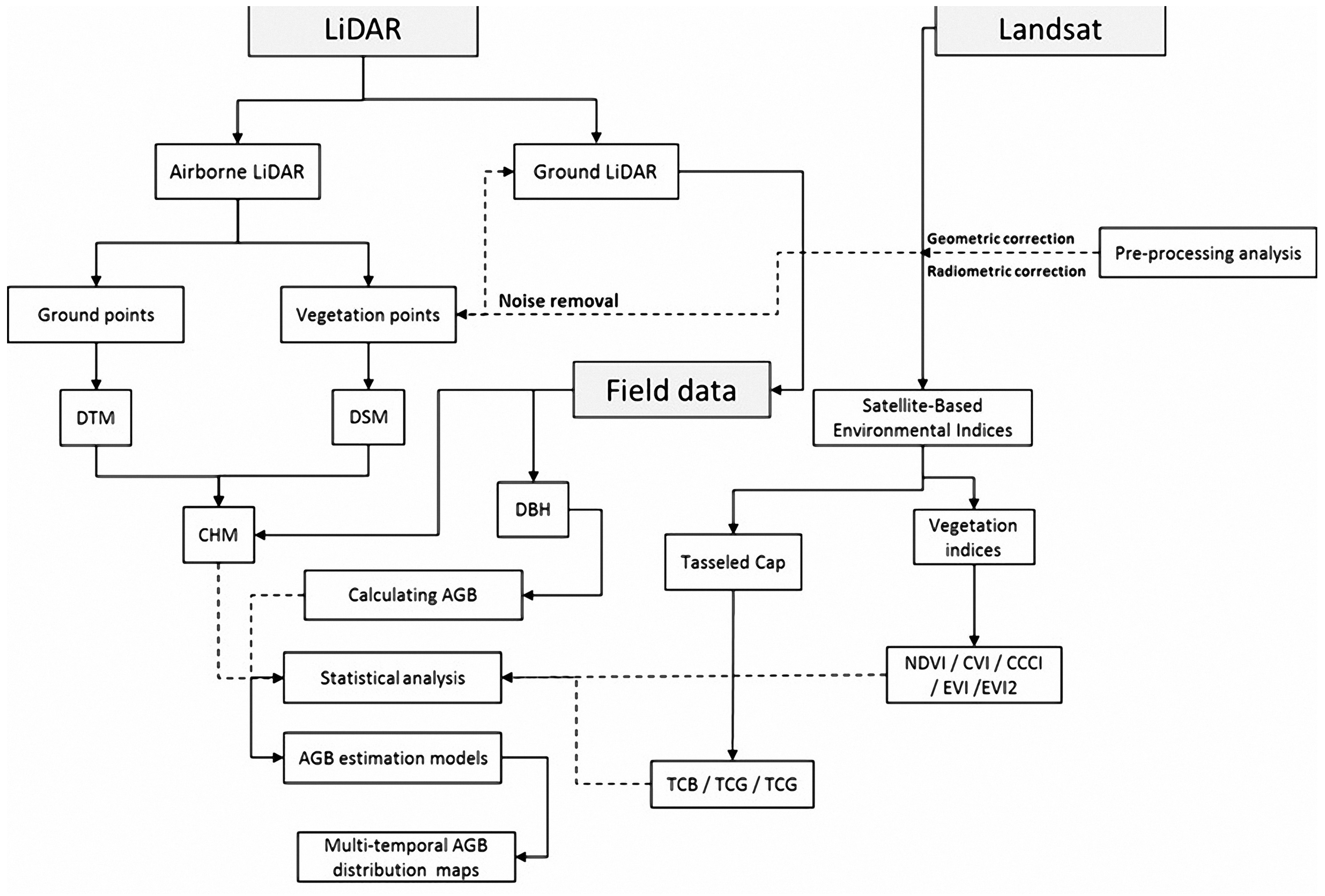
3. Materials and Methods

This investigation is based on various remote sensing data that were acquired and integrated via advanced analytical techniques, as shown in Figure 2. The spatial analyses were conducted using several datasets (i.e., multi-temporal Landsat satellite images, high-resolution ground LiDAR, and airborne LiDAR). The integration system analyses were conducted after the pre-processing data quality check to remove the noise and unify the data geo-references. Software packages, such as ArcGIS 10.1, Cyclone 8.11, and ENVI 5.0, were used to achieve the objectives.

Figure 1. The geographical location of the case study, aerial imagery with 0.5 m spatial resolution.

Figure 1. The geographical location of the case study, aerial imagery with 0.5 m spatial resolution.

Figure 2. Flow chart describing the integration and the analyses steps of Landsat and LiDAR data.

Figure 2. Flow chart describing the integration and the analyses steps of Landsat and LiDAR data.

3.1. Airborne LiDAR and Canopy Height Extraction

The discrete airborne LiDAR data for the case study were acquired on 22 November 2005 and 26 March 2006. The horizontal root-mean-square error (RMS) is 45 cm, and the vertical RMS is 30 cm. The point density of the acquired LiDAR data for all tiles is greater than 1.3 points per square meter. Environmental System Research Institute (ESRI) ArcGIS 10.1 was used to process the LAS v1.0 point cloud, which contained all return point clouds. Digital elevation models (DEM) and digital surface models (DSM) were produced after removing the noise from the data acquisition. A canopy height model (CHM) with one meter spatial resolution was calculated by subtracting the DEM from DSM; the CHM represents a 3D surface of the vegetation cover.

3.2. Ground LiDAR and Field Measurements

The forest biophysical parameters were collected on 20 May and 11 July 2014, using Leica ScanStation C10. An exploratory field survey was conducted on 28 April 2014, to locate the scan stations that represent the overall ecosystem of the case study. Eight scan stations were placed at three locations, where the range of the trees metrics was 300 m and the scan rate was 50,000 points/s. The scan stations are fully operational in conditions ranging from bright sunlight to complete darkness, and the accuracy of single tree’s (object) measurements was 4–6 mm. Cyclone 8.11 software was used to calculate the following characteristics of individual trees: diameter at breast height (DBH), height (H), and canopy width. One of the major advantages of using ground LiDAR is that the obtained data do not require extra field surveys for validation [38,39].

3.3. Landsat Data

Landsat 5 Thematic Mapper TM satellite images in cloud-free conditions were obtained from the US Geological Survey for spring and summer days in five years, i.e., 2 September 1988, 15 September 1990, 28 May 2005, 27 August 2009, and 9 September 2011. The Landsat data were re-projected into a Universal Transverse Mercator (UTM), zone 11 north NAD 1983 horizontal coordinate system. ENVI version 5.0 was used to apply the radiometric correction analysis to all multi-temporal Landsat data using the Landsat calibration utility for atmospheric correction. The calibrated images provide better reflectance for minimizing the climate effects that could potentially lead to miscalculations or additional noise. The small temporal heterogeneity (less than three months) between the Landsat dataset will not affect the change detection analysis because of the slow rate of growth in coniferous species [40,41].

3.4. Calculating the Spectral Indices

The normalized difference vegetation index (NDVI), enhanced vegetation index (EVI and EVI2), chlorophyll vegetation index (CVI), and tasseled cap transformation were considered as vegetation spectral indices (VSIs). These indices were estimated from the multi-temporal Landsat satellite data (Table 1), which were integrated with the ground LiDAR measurements to obtain the biophysical parameters of the studied forest; the parameters were used to estimate the biomass. The VSIs were statistically related to the biomass status and spatial distribution and were resistant to atmospheric influences and the forest structure [16,17,42,43,44].

Tasseled cap transformations are considered to be robust indicators of forest dynamics [50]. A linear combination of sensor-specific weightings for each band (Table 2) was applied to the multi-temporal Landsat 5 satellite images; these transformations are the three orthogonal indices called brightness, greenness and wetness (TCB, TCG and TCW, respectively) [20,51].

Table 1. The derived VSIs equations from Landsat 5 TM, ${\rho }_{NIR}$ is the near infrared band, ${\rho }_R$ is the red band, ${\rho }_B$ is the blue band, and ${\rho }_G$ is the green band. G, C₁, C₂, and L are 2.5, 6, 7.5, and 1 respectively.

Spectral Index	Formula	Reference
$NDVI$	$\frac{{\text{ρ}}_{NIR}- {\text{ρ}}_R}{{\text{ρ}}_{NIR}+{\text{ρ}}_R}$	[45]
$EVI$	$G\frac{{\text{ρ}}_{NIR}- {\text{ρ}}_R}{{\text{ρ}}_{NIR}+C_1{\rho }_R-C_2{\text{ρ}}_B+L}$	[46,47]
$EVI2$	$2.5 \frac{{\text{ρ}}_{NIR}-{\text{ρ}}_R}{{\text{ρ}}_{NIR}+ 2.4{\text{ρ}}_R+L}$	[15]
$CVI$	$\frac{{\text{ρ}}_{NIR} \times {\text{ρ}}_R}{{\text{ρ}}_G^2}$	[48,49]

Table 1. The derived VSIs equations from Landsat 5 TM, ${\rho }_{NIR}$ is the near infrared band, ${\rho }_R$ is the red band, ${\rho }_B$ is the blue band, and ${\rho }_G$ is the green band. G, C₁, C₂, and L are 2.5, 6, 7.5, and 1 respectively.

Spectral Index	Formula	Reference
$NDVI$	$\frac{{\text{ρ}}_{NIR}- {\text{ρ}}_R}{{\text{ρ}}_{NIR}+{\text{ρ}}_R}$	[45]
$EVI$	$G\frac{{\text{ρ}}_{NIR}- {\text{ρ}}_R}{{\text{ρ}}_{NIR}+C_1{\rho }_R-C_2{\text{ρ}}_B+L}$	[46,47]
$EVI2$	$2.5 \frac{{\text{ρ}}_{NIR}-{\text{ρ}}_R}{{\text{ρ}}_{NIR}+ 2.4{\text{ρ}}_R+L}$	[15]
$CVI$	$\frac{{\text{ρ}}_{NIR} \times {\text{ρ}}_R}{{\text{ρ}}_G^2}$	[48,49]

Table 2. Landsat 5 TM band-specific weights for TCB,TCG and TCW.

Tasseled Cap Feature	Weighting for Tasseled Cap Transformation Using Landsat 5 TM Dataset
	B1	B2	B3	B4	B5	B7
Brightness	0.3037	0.2793	0.4343	0.5585	0.5082	0.1863
Greenness	−0.2848	−0.2435	−0.5436	0.7243	0.0840	−0.1800
Wetness	0.1509	0.1793	0.3299	0.3406	−0.7112	−0.4572

Table 2. Landsat 5 TM band-specific weights for TCB,TCG and TCW.

Tasseled Cap Feature	Weighting for Tasseled Cap Transformation Using Landsat 5 TM Dataset
	B1	B2	B3	B4	B5	B7
Brightness	0.3037	0.2793	0.4343	0.5585	0.5082	0.1863
Greenness	−0.2848	−0.2435	−0.5436	0.7243	0.0840	−0.1800
Wetness	0.1509	0.1793	0.3299	0.3406	−0.7112	−0.4572

3.5. Allometric Equations and Ground LiDAR Metrics from Individual Trees and Point Clouds

The Jenkins allometric equations model are suitable for predicting the biomass based on DBH for different coniferous species [26,27,28], Jenkins et al. [22] estimated the biomass as follow:

$$B_i=exp\left({\text{β}}_0+{\text{β}}_{1}ln(DBH)\right)$$

(1)

where $B_i$ is the biomass (kg), $DBH$ is the diameter in meters at breast height (1.3 m), $ln$ is the natural log base, and ${\text{β}}_0,{\text{ β}}_1$ are the coefficients.

Also, Lambert et al. [52] and Ung et al. [53] provided allometric equations to estimate biomass were derived from thousands of samples (trees) across Canada [54]. The allometric equation form is shown as follows:

$$Y_i= {\text{β}}_{1}DB{H}^{{\text{β}}_2}{H}^{{\text{β}}_3}$$

(2)

where $Y_i$ is the biomass (kg), ${\text{β}}_1,{\text{ β}}_2,{\text{ β}}_3$ are the coefficients.

Ni-Meister et al. [8] Found that LiDAR metrics can be used as predictors for biomass. In this study, we used a new high-resolution ground LiDAR to obtain the relationship between the DBH and the tree height (H) in tree-level metric bases (r² = 0.74; p < 0.001). Approximately 700 individual trees in the coniferous forest were obtained in the study site (Figure 3), and the empirical relationships from the ground LiDAR field measurements were developed as follows:

$$DBH=0.098\times H-0.055$$

(3)

where DBH is the diameter in meters at breast height (at 1.3 m) and H is the tree height in meters.

Figure 3. A 3D visualization of the data obtained from the high resolution ground LiDAR.

Figure 3. A 3D visualization of the data obtained from the high resolution ground LiDAR.

3.6. Statistical and Temporal Trend Analysis

The stepwise multiple linear regression method was used to select the most significant variables; multiple linear regressions were conducted for airborne LiDAR and derived VSI from Landsat 5 data for 2005. We determined the most suitable model, which is based on the linear regression scatter plot with the ground LiDAR results that identified the biophysical metrics for the study. This model was used to predict H for the years of 1988, 1990, 2009, and 2011 and to map the biomass in the study years. The conventional multivariate regression model can be expressed as follows:

$$y= x_0+a_1{x}_1+\dots +a_i{x}_i$$

(4)

where $y$ is CHM in meters and is considered to be the dependent parameter to be predicted, $x_0$ is the intercept, $a_1{x}_1$ are the regression coefficients and the values of the independent variables, and $i$ is the number of independent variables.

To determine the model that best predicted the biomass spatial distribution, 409 points were used to validate the prediction models; we used the root mean square error (RMSE), which indicates how far the predicted values deviated from the measured data (ground LiDAR) [55].

$$RMSE=\sqrt{\frac{1}{N}{\displaystyle \sum }_{i=1}^N{\left(y_0-y_i\right)}^2}$$

(5)

where $y_0$ is the predicted values, $y_i$ is the measured values from the ground LiDAR, and $N$ is the number of the observations and grid points.

The Akaike’s Information Criterion (AIC) can be defined as the objective way to decide between models that provide best fits, and recently used as an assessment tool to select the best model that predict/or estimate phenomena [56].

$$AIC=-2lnL+2k$$

(6)

where $lnL$ is the maximized log-likelihood of the model and $k$ is the number of parameters estimated [57].

$$\mathrm{\Delta }AI{C}_i=AI{C}_i-AI{C}_{min}$$

(7)

Also, AIC differences can be used to identify the best model that has$\mathrm{\Delta }AI{C}_i\equiv 0$, where $AI{C}_i$ is the Akaike of model $i$ and $AI{C}_{min}$ is the lowest Akaike among the tested models $i$.

A pixel-based image comparison was used to estimate the amount of change over the study years. Four temporal subsets were analyzed: 1988–1990, 1990–2005, 2005–2009, and 2009–2011. The comparisons were based on the difference between the same spatial pixel positions for each pair of multi-year periods. The difference between each pair provides useful data on the most degraded or reclaimed sites in the study area [58,59]. A temporal trend analysis was provided by [17]. The Mann-Kendall trend test analysis is a nonparametric test for linear regression with zero slopes. Each pixel location was calculated in a time series; the S statistics increase when the value of the later data is higher than the earlier data, and the cumulative score of all pairs is used to calculate S [60]. Gilbert [61] proposed the following procedures to calculate the Mann-Kendall trend statistics:

(1)

The biomass data should be listed in temporal order:

$$x_1,x_2,\dots ,x_n\text{ where }{x}_i\text{ is the biomass estimated maps at time }i$$

(2)

The sign $(x_j-x_k)$ is the indicator function, where the value of all $n\left(n-1\right)/2$ must be determined for all differences of $x_j-x_k$ where $j>k.$

$$\text{sign}\left(x_j-x_k\right)=\{\begin{array}{c}+1 if x_j-x_k>0\\ 0 if x_j-x_k=0\\ -1 if x_j-x_k<0\end{array}$$

(8)

(3)

Computing the Mann-Kendall Statistics as follow:

$$\text{S}={\displaystyle \sum }_{k=1}^{n-1}{\displaystyle \sum }_{ j=k+1}^n\text{sign }(x_j-x_k)$$

(9)

4. Results

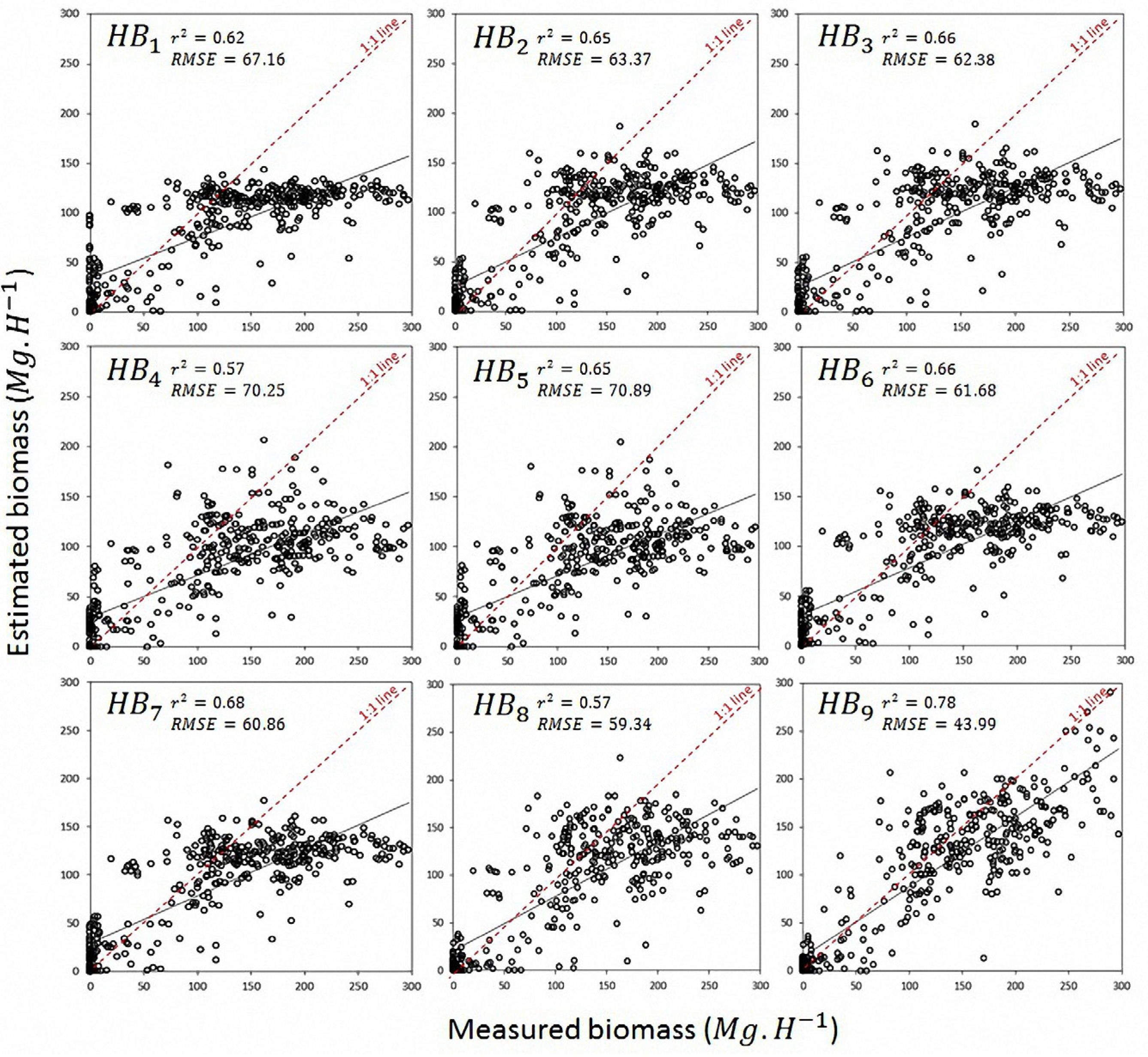
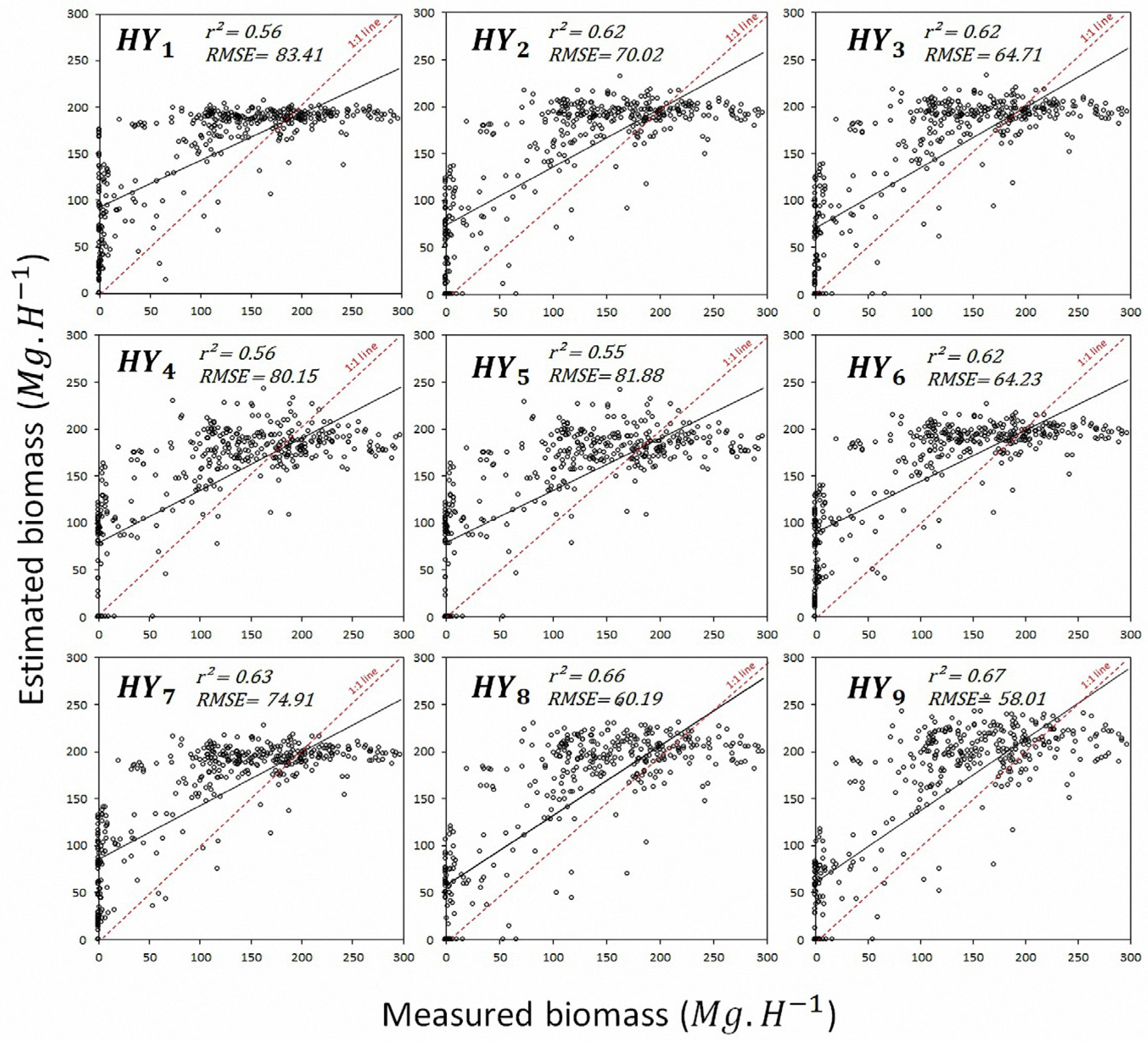
4.1. Regression Models and Biomass Estimation

Stepwise multiple regression analysis was used to estimate the canopy height from the Landsat spectral indices (NDVI, EVI2, TCW, TCG, and TCB), which are independent variables. Nine models were established to identify the best relationship between the airborne LiDAR and Landsat data for 2005 from 4771 points that were extracted from all variables at the same location. H₈ and H₉ were the best models for estimating the canopy height (r² = 0.73, and 0.74; p < 0.001, respectively. $\mathrm{\Delta }AI{C}_i=0$ and 176.4, respectively), as shown in Table 3.

The final equations that were used to predict the biomass directly from canopy height are shown as follow:

$$B_i=exp\left(0.1617+2.142\times Ln[0.098\times H_i-0.055]\right)$$

(10)

$$Y_i= 22.82 \times {(0.098 \times H_i-0.055)}^{0.05612}{H_i}^{0.8931}$$

(11)

where $B_i$ is the biomass in Mg∙H⁻¹ based on the Jenkins allometric equation, $Y_i$ is the biomass in Mg∙H⁻¹ based on the Lambert and Ung allometric equation, and $H_i$ is the canopy height in meters.

Table 3. A summary of multiple regression analysis results and regression models.

Variables	Models	R2	$\mathrm{\Delta } AI{C}_i$
$TCB, TCG, TCW$	$H_1=18.67-0.13\times TCB+0.15\times TCG-0.04\times TCW$	0.67	1047.81
$TCB,TCW,NDVI$	$H_2=8.40+21.13\times NDVI-0.08\times TCB-0.04\times TCW$	0.70	618.22
$TCB,TCW,EVI2$	$H_3=8.54+8.52\times EVI2-0.08\times TCB-0.04\times TCW$	0.70	621.35
$TCW,NDVI$	$H_4= -0.75+27.36\times NDVI+0.02\times TCW$	0.66	1265.23
$TCW,EVI2$	$H_5=-0.67+10.98\times EVI2+0.02\times TCW$	0.66	1287.59
$TCB,NDVI$	$H_6=9.04+16.39\times NDVI-0.06\times TCB$	0.69	722.51
$TCB,EVI2$	$H_7=9.17+6.58\times EVI2-0.06\times TCB$	0.69	727.05
$TCB,TCG,NDVI$	$H_8=-6.12+0.01\times TCB-0.38\times TCG+54\times NDVI$	0.73	176.4
$TCB,TCG,TCW,EVI2$	$H_9= -14.79-0.63\times TCG+28.57\times EVI2+0.09\times TCB+0.07\times TCW$	0.74	0

Table 3. A summary of multiple regression analysis results and regression models.

Variables	Models	R2	$\mathrm{\Delta } AI{C}_i$
$TCB, TCG, TCW$	$H_1=18.67-0.13\times TCB+0.15\times TCG-0.04\times TCW$	0.67	1047.81
$TCB,TCW,NDVI$	$H_2=8.40+21.13\times NDVI-0.08\times TCB-0.04\times TCW$	0.70	618.22
$TCB,TCW,EVI2$	$H_3=8.54+8.52\times EVI2-0.08\times TCB-0.04\times TCW$	0.70	621.35
$TCW,NDVI$	$H_4= -0.75+27.36\times NDVI+0.02\times TCW$	0.66	1265.23
$TCW,EVI2$	$H_5=-0.67+10.98\times EVI2+0.02\times TCW$	0.66	1287.59
$TCB,NDVI$	$H_6=9.04+16.39\times NDVI-0.06\times TCB$	0.69	722.51
$TCB,EVI2$	$H_7=9.17+6.58\times EVI2-0.06\times TCB$	0.69	727.05
$TCB,TCG,NDVI$	$H_8=-6.12+0.01\times TCB-0.38\times TCG+54\times NDVI$	0.73	176.4
$TCB,TCG,TCW,EVI2$	$H_9= -14.79-0.63\times TCG+28.57\times EVI2+0.09\times TCB+0.07\times TCW$	0.74	0

Figure 4 shows the comparisons between the measured biomass from the high-resolution ground LiDAR and the estimated biomass derived from the Landsat spectral indices models. The models with higher adjusted r² and lower RMSE are indicative of better biomass estimations from the spectral indices variables; the models (HB₇ and HB₉) with higher r² values had lower RMSE values. TCG and TCW increased r² + 0.1, and the RMSE decreased (−16.87 Mg/H). Also, the Lambert and Ung allometric equation provided the same superior models (HY₇ and HY₉), see Figure 5.

Figure 4. The stepwise multiple linear regression results for the measured and estimated biomass analysis of nine different models $H_i$ (see, Table 3), and based on Jenkins allometric equation $B_i$.

Figure 4. The stepwise multiple linear regression results for the measured and estimated biomass analysis of nine different models $H_i$ (see, Table 3), and based on Jenkins allometric equation $B_i$.

Figure 5. The stepwise multiple linear regression results for the measured and estimated biomass analysis of nine different models $H_i$ (see, Table 3), and based on Lambert and Ung allometric equation $Y_i$.

Figure 5. The stepwise multiple linear regression results for the measured and estimated biomass analysis of nine different models $H_i$ (see, Table 3), and based on Lambert and Ung allometric equation $Y_i$.

4.2. Estimation Uncertainties

Understanding, identifying, and reducing the sources of uncertainties are critical in improving forest biomass estimation performances. In this investigation, based on the ground LiDAR data survey, a group of statistical models was developed. The models were based on the best relationships between the tree height data, DBH and spectral indices to estimate biomass from the Landsat images. However, our models involve uncertainty for the following reasons. First, a scale difference exists between remotely sensed data and ground LiDAR survey data. The spatial resolution of Landsat 5 data is 30 m. Considering the high-resolution ground LiDAR scans, the average values of multiple samples were used to reduce the estimation error caused by the scale difference. Second, the satellite image data used in this study originate from Landsat 5 and require an atmospheric correction to obtain the best spectral reflectance for surface greenness and distribution. Third, there are uncertainties concerning the field survey for biomass change detection because simultaneous field data and satellite images are difficult to obtain. To address the temporal variance between the field survey and the remote sensing data acquisition, we focused on the relationships between the biophysical parameters in the study sites rather than the temporal data acquisition; the ultimate goal of our research is to provide an optimal biomass prediction model.

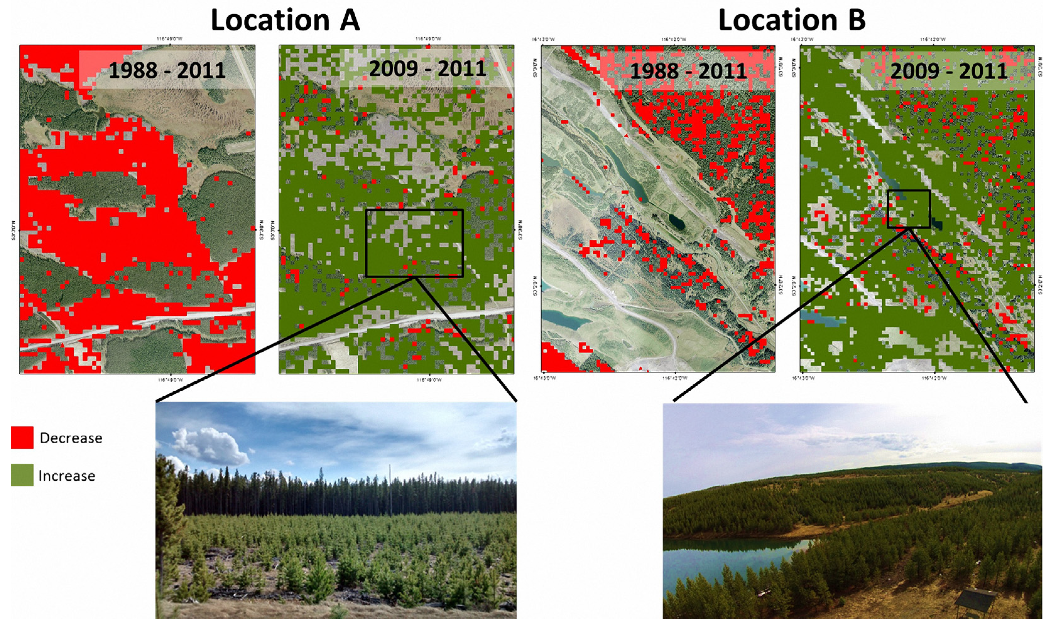
4.3. Biomass Spatial Distribution and Trajectory of Change

The estimated biomass results had a wide ranging spatial distribution as a result of mining activities that led to deforestation, as shown in Figure 6. During 1988–1990, the total area with a biomass <100 Mg/H decreased approximately 55.3%, and the biomass in the southeastern area increased approximately 36.8%. The northwestern and eastern areas lost approximately 2.2% of the >600 Mg/H biomass area, which shows the capability of the estimation model that was used to map the biomass spatial distribution. The study site was massively deforested, except for the northeastern side. After 2005, land reclamation occurred. During 2005–2009, the vegetation cover area increased 26.6% for the trees that had biomass >600 Mg/H, 25.4% for biomass of 100–250 Mg/H, and 23% for biomass <100 Mg/H. The biomass of trees <100 Mg/H increased 57.8% as a result of continuous land reclamation and regrowth.

As shown in Figure 7, a trend analysis for 1988–2011 was conducted using the estimated biomass data; the analysis showed a significant decrease in the biomass over this 23-year period. Applying the biomass prediction model to the S statistics provided clear information on how massively the mining activities deforested huge areas for this period. Changing the time window provided a different view of the activities at the same study sites. During 2009–2011, the trend analysis showed an obvious increase in the biomass, which is clear evidence of reclamation activity and regrowth.

5. Discussion

5.1. Major Findings

The integration of data from optical remote sensing and airborne and ground LiDAR provided the ultimate data source for estimating and mapping the spatial and temporal biomass distribution for coniferous forests. Many scientists have demonstrated that Landsat and LiDAR data can be used to derive highly reliable maps of biomass distributions based on field survey measurements [3,16,50].

Figure 6. The spatial distribution of the estimated biomass over the case study over the years 1988, 1990, 2005, 2009, and 2011; the spatial resolution is 30 m.

Figure 6. The spatial distribution of the estimated biomass over the case study over the years 1988, 1990, 2005, 2009, and 2011; the spatial resolution is 30 m.

Figure 7. A zoomed view of two sites in the case study showing the decrease and increase of the biomass for long-term (1988–2011) and short-term (2009–2011).

Figure 7. A zoomed view of two sites in the case study showing the decrease and increase of the biomass for long-term (1988–2011) and short-term (2009–2011).

In this study, we developed an approach that further integrates airborne LiDAR data with the high-resolution ground LiDAR to specifically determine the relationships between the biophysical characteristics of a forest and spectral indices from Landsat data. The relationships were used to directly estimate the biomass distribution at the study site from the spectral indices that were calculated from multi-temporal Landsat satellite images. Several key elements were considered to estimate and map the biomass temporal dynamics and spatial distribution using Landsat data. First, information and statistical relationships derived from both the airborne and high-resolution ground LiDAR were used to improve the biomass modeling substantially and provide accurate datasets. The advantage of using ground LiDAR for biomass modeling is the capability of accurately measuring all the biophysical details at the study site and of linking the ground LIDAR data to the airborne LiDAR data. This connection revealed information undetectable from airborne LiDAR; thus, this information is essential to provide the best model for estimating biomass directly from optical remote sensing data, such as Landsat satellite data. Second, spectral indices were carefully chosen to provide more information on the vegetation cover, as shown in Table 1 and Table 2. In this research, VSIs were derived from calibrated multi-temporal Landsat images to detect and map the location and magnitude of biomass dynamics. Several studies demonstrated the benefit of using Landsat images for change detection in coniferous forest environments [62]. We provide new information on the potential use and capability of such methods in estimating and mapping biomass dynamics. Third, the modeling approach has a high degree of certainty, based on the direct link between spectral indices and biophysical parameters captured by the airborne and ground LiDAR. TCB, TCG, TCW, EVI2, and NDVI were highly suitable variables for estimating the biomass spatial distribution for our case study, as shown in Table 3. Similarly to [17], a strong, negative relationship was found between brightness reflectance and vegetation coverage (r = 0.81); this relationship represents the bare soil spots that result from the mining activities in the study site. The TCW is a highly weighted (positively) spectral variable with CHM (r =0.78); this relationship supported the modeling approach to estimate the biomass according to the canopy heights [13,27]. Fourth, Zhao et al. [28] stated that the multiple linear models with height-related metrics estimate the biomass variation better than the profile-related metrics because the biomass is directly related to the height and/or DBH, whereas the canopy-profile-based metrics provide very limited information. Essentially, the Jenkins allometric equations used in this research employs DBH as the input, but it is still possible to use an additional variable (i.e., height), as suggested by [27,28].

Models with higher adjusted r² and low RMSE likely have a greater ability to predict biomass using LiDAR-derived variables. HB₉ and HY₉ were the best models regarding biomass estimations using allometric equations. The final regression model HB₉ was further used with the multi-temporal Landsat images to estimate the biomass spatial distribution; this model is useful for cases that have intense coniferous forests. Additionally, these results showed the advantages of using Landsat satellite images to map and assess biomass change over time and to detect deforestation and reclamation effects (see Figure 6). Finally, change detection provides more information on the history of the study site in terms of the trajectory of change. Massive anthropogenic activity appeared in 2005 throughout the study site. The northeastern side of the study site, which has a high elevation, showed more vegetation cover stability, which is a morphological characteristic that protects trees from the mining activities. In 2004, mining activities increased to nearly 4 million tons/year, and the mining reached its full extent in the summer of 2006, in which thermal coal production doubled [35]. During 1990–2005, the areas that had a biomass <100 Mg/H decreased to 90.3%, and the areas that had a biomass >600 Mg/H decreased by 7.2%.

5.2. Suggestions for Future Research

This research successfully used multi-temporal Landsat data to develop and introduce a new methodology for assessing biomass change in coniferous forests in human-affected areas; nevertheless, some aspects need to be considered in future research. Landsat satellite data provide the most continuous time series for assessing biomass change. However, it is highly preferable to use continuous multi-temporal satellite data in bi-weekly temporal intervals to avoid possible disturbances/or natural hazards (wildfires, floods, etc.) that could affect the findings. Integrating different sensors could cause errors due to spatial resolution heterogeneity, and therefore, any integration approaches in environmental research must be taken gradually by developing the integration analysis in a stepwise manner and assessing the accuracy of each step. We believe that integrating ground LiDAR directly with Landsat data will result in more errors rather than greater accuracy. A field survey is essential to verify the findings and to confirm whether the predictions correspond with reality. The use of high-resolution optical satellite sensors (Worldview, Quick Bird, and Spot) is a significant advantage of this type of research, but these data are costly compared with the free Landsat archive.

6. Conclusions

In this study, we estimated the multi-temporal and spatial distribution of biomass for a coniferous forest at a coal mining site to assess the biomass changes as a result of land degradation and reclamation. Various datasets and techniques were used and integrated to provide the best predictors for estimating biomass directly from Landsat data. Ground LiDAR metrics were essential to understanding and accurately finding the best relationship between different biophysical parameters in our case study. A strong relationship (r² = 0.74; p < 0.001) was found between tree height and DBH; this statistical relationship was based on the metrics of 700 individual trees. The ground-LiDAR-based regression model was used to replace the DBH in Jenkins allometric equation with the tree height, which was obtained from airborne LiDAR. This step helped estimate the biomass from the airborne LiDAR for 2005 directly from the tree height that was extracted from the difference between the DEM and DSM. Nine spectral based models were analyzed with the airborne LiDAR metrics to select the best biomass predictor; HB₉ proved to be the best predictor (r² = 0.78; RMSE = 44 Mg/H; p < 0.001). This model was used to estimate the biomass spatial distributions for 1988, 1990, 2001, 2005, and 2011. A major loss of biomass was found in 2005, when the study site lost approximately 50% of its forested area. This major deforestation was the result of extreme excavation. The land morphology in the northeastern side of the site played a vital role in protecting the natural habitats from the excavation activity. The areas with biomass <100 Mg/H were indicators for land reclamation and conservation, both of which increased dramatically during 2005–2011. Predicting biomass from Landsat data requires different resolution levels of data records that can be integrated for understanding the disturbance activity that occurred. With the continuity of the Landsat data, developing new algorithms becomes highly essential for studying historical changes and understanding the connection between past and current environmental states [20].

References

1. He, Q.; Chen, E.; An, R.; Li, Y. Above-Ground biomass and biomass components estimation using LiDAR data in a coniferous forest. Forests 2013, 4, 984–1002. [Google Scholar] [CrossRef]
2. Fernández-Manso, O.; Fernández-Manso, A.; Quintano, C. Estimation of aboveground biomass in Mediterranean forests by statistical modelling of ASTER fraction images. Int. J. Appl. Earth Obs. Geoinf. 2014, 31, 45–56. [Google Scholar] [CrossRef]
3. Pflugmacher, D.; Cohen, W.B.; Kennedy, R.E.; Yang, Z. Using landsat-derived disturbance and recovery history and LiDAR to map forest biomass dynamics. Remote Sens. Environ. 2014, 151, 124–137. [Google Scholar] [CrossRef]
4. Deng, S.; Katoh, M.; Guan, Q.; Yin, N.; Li, M. Estimating forest aboveground biomass by combining ALOS PALSAR and WorldView-2 data: A case study at Purple Mountain National Park, Nanjing, China. Remote Sens. 2014, 6, 7878–7910. [Google Scholar] [CrossRef]
5. Laurin, G.V.; Chen, Q.; Lindsell, J.A.; Coomes, D.A.; del Frate, F.; Guerriero, L.; Pirotti, F.; Valentini, R. Above ground biomass estimation in an African tropical forest with LiDAR and hyperspectral data. ISPRS J. Photogramm. Remote Sens. 2014, 89, 49–58. [Google Scholar] [CrossRef]
6. Kwak, D.A.; Lee, W.K.; Lee, J.H.; Biging, G.S.; Gong, P. Detection of individual trees and estimation of tree height using LiDAR data. J. For. Res. 2007, 12, 425–434. [Google Scholar] [CrossRef]
7. Cao, L.; Coops, N.; Hermosilla, T.; Innes, J.; Dai, J.; She, G. Using small-footprint discrete and full-waveform airborne LiDAR metrics to estimate total biomass and biomass components in subtropical forests. Remote Sens. 2014, 6, 7110–7135. [Google Scholar] [CrossRef]
8. Ni-Meister, W.; Lee, S.; Strahler, A.H.; Woodcock, C.E.; Schaaf, C.; Yao, T.; Ranson, K.J.; Sun, G.; Blair, J.B. Assessing general relationships between aboveground biomass and vegetation structure parameters for improved carbon estimate from lidar remote sensing. J. Geophys. Res. 2010, 115, G00E11. [Google Scholar] [CrossRef]
9. Edson, C.; Wing, M.G. Airborne Light Detection and Ranging (LiDAR) for individual tree stem location, height, and biomass measurements. Remote Sens. 2011, 3, 2494–2528. [Google Scholar] [CrossRef] [Green Version]
10. Kim, Y.; Yang, Z.; Cohen, W.B.; Pflugmacher, D.; Lauver, C.L.; Vankat, J.L. Distinguishing between live and dead standing tree biomass on the North Rim of Grand Canyon National Park, USA using small-footprint LiDAR data. Remote Sens. Environ. 2009, 113, 2499–2510. [Google Scholar] [CrossRef]
11. Dandois, J.P.; Ellis, E.C. Remote sensing of vegetation structure using computer vision. Remote Sens. 2010, 2, 1157–1176. [Google Scholar] [CrossRef]
12. Seielstad, C.; Stonesifer, C.; Rowell, E.; Queen, L. Deriving fuel mass by size class in Douglas-fir (Pseudotsuga menziesii) using terrestrial laser scanning. Remote Sens. 2011, 3, 1691–1709. [Google Scholar] [CrossRef]
13. Lu, D.; Chen, Q.; Wang, G.; Moran, E.; Batistella, M.; Zhang, M.; Laurin, G.V.; Saah, D. Aboveground forest biomass estimation with landsat and LiDAR data and uncertainty analysis of the estimates. Int. J. For. Res. 2012, 2012, 1–16. [Google Scholar]
14. Kelsey, K.; Neff, J. Estimates of aboveground biomass from texture analysis of landsat imagery. Remote Sens. 2014, 6, 6407–6422. [Google Scholar] [CrossRef]
15. Miura, T.; Yoshioka, H.; Fujiwara, K.; Yamamoto, H. Inter-Comparison of ASTER and MODIS surface reflectance and vegetation index products for synergistic applications to natural resource monitoring. Sensors 2008, 8, 2480–2499. [Google Scholar] [CrossRef]
16. Chen, X.; Vierling, L.; Rowell, E.; DeFelice, T. Using LiDAR and effective LAI data to evaluate IKONOS and Landsat 7 ETM+ vegetation cover estimates in a ponderosa pine forest. Remote Sens. Environ. 2004, 91, 14–26. [Google Scholar] [CrossRef]
17. Czerwinski, C.J.; King, D.J.; Mitchell, S.W. Mapping forest growth and decline in a temperate mixed forest using temporal trend analysis of Landsat imagery, 1987–2010. Remote Sens. Environ. 2014, 141, 188–200. [Google Scholar] [CrossRef]
18. Mitchard, E.T.A; Saatchi, S.S.; Lewis, S.L.; Feldpausch, T.R.; Gerard, F.F.; Woodhouse, I.H.; Meir, P. Comment on A first map of tropical Africa’s above-ground biomass derived from satellite imagery. Environ. Res. Lett. 2011, 6, 49001. [Google Scholar] [CrossRef]
19. Zhang, G.; Ganguly, S.; Nemani, R.R.; White, M.A.; Milesi, C.; Hashimoto, H.; Wang, W.; Saatchi, S.; Yu, Y.; Myneni, R.B. Estimation of forest aboveground biomass in California using canopy height and leaf area index estimated from satellite data. Remote Sens. Environ. 2014, 151, 44–56. [Google Scholar] [CrossRef]
20. Pflugmacher, D.; Cohen, W.B.; E. Kennedy, R. Using Landsat-derived disturbance history (1972–2010) to predict current forest structure. Remote Sens. Environ. 2012, 122, 146–165. [Google Scholar] [CrossRef]
21. Zhang, X.; Kondragunta, S. Estimating forest biomass in the USA using generalized allometric models and MODIS land products. Geophys. Res. Lett. 2006, 33, L09402. [Google Scholar]
22. Jenkins, J.C.; Chojnacky, D.C.; Heath, L.S.; Birdsey, R.A. National-Scale biomass estimators for united states tree species. For. Sci. 2003, 49, 12–35. [Google Scholar]
23. Jenkins, J.C.; Chojnacky, D.C.; Heath, L.S.; Birdsey, R.A. Comprehensive Database of Diameter-Based Biomass Regressions for North American Tree Species; USDA Forest Service: Pennsylvania, USA, 2004; p. 48.
24. Jenkins, J.C.; Birdsey, R.A.; Pan, Y. Biomass and NPP estimation for the mid-atlantic region (USA) using plot-level forest inventory data. Ecol. Appl. 2001, 11, 1174–1193. [Google Scholar] [CrossRef]
25. Ahmed, R.; Siqueira, P.; Hensley, S.; Bergen, K. Uncertainty of forest biomass estimates in North temperate forests due to allometry: Implications for remote sensing. Remote Sens. 2013, 5, 3007–3036. [Google Scholar] [CrossRef]
26. Yoon, T.K.; Park, C.W.; Lee, S.J.; Ko, S.; Kim, K.N.; Son, Y.; Lee, K.H.; Oh, S.; Lee, W.K.; Son, Y. Allometric equations for estimating the aboveground volume of five common urban street tree species in Daegu, Korea. Urban For. Urban Green. 2013, 12, 344–349. [Google Scholar] [CrossRef]
27. Paul, K.I.; Roxburgh, S.H.; Ritson, P.; Brooksbank, K.; England, J.R.; Larmour, J.S.; Raison, R.J.; Peck, A.; Wildy, D.T.; Sudmeyer, R.A.; et al. Testing allometric equations for prediction of above-ground biomass of mallee eucalypts in southern Australia. For. Ecol. Manag. 2013, 310, 1005–1015. [Google Scholar] [CrossRef]
28. Zhao, F.; Guo, Q.; Kelly, M. Allometric equation choice impacts LiDAR-based forest biomass estimates: A case study from the Sierra National Forest, CA. Agric. For. Meteorol. 2012, 165, 64–72. [Google Scholar] [CrossRef]
29. Ter-Mikaelian, M.T.; Korzukhin, M.D. Biomass equations for sixty-five North American tree species. For. Ecol. Manag. 1997, 97, 1–24. [Google Scholar] [CrossRef]
30. Hyde, P.; Nelson, R.; Kimes, D.; Levine, E. Exploring LiDAR–RaDAR synergy—predicting aboveground biomass in a southwestern ponderosa pine forest using LiDAR, SAR and InSAR. Remote Sens. Environ. 2007, 106, 28–38. [Google Scholar] [CrossRef]
31. Popescu, S.C. Estimating biomass of individual pine trees using airborne LiDAR. Biomass Bioenergy 2007, 31, 646–655. [Google Scholar] [CrossRef]
32. Sonter, L.J.; Moran, C.J.; Barrett, D.J.; Soares-Filho, B.S. Processes of land use change in mining regions. J. Clean. Prod. 2014, 84, 494–501. [Google Scholar] [CrossRef] [Green Version]
33. Cheng, W.; Bian, Z.; Dong, J.; Lei, S. Soil properties in reclaimed farmland by filling subsidence basin due to underground coal mining with mineral wastes in China. Trans. Nonferrous Met. Soc. China 2014, 24, 2627–2635. [Google Scholar] [CrossRef]
34. Pietrzykowski, M.; Daniels, W.L. Estimation of carbon sequestration by pine (Pinus sylvestris L.) ecosystems developed on reforested post-mining sites in Poland on differing mine soil substrates. Ecol. Eng. 2014, 73, 209–218. [Google Scholar]
35. Strong, W.L. Vegetation development on reclaimed lands in the Coal Valley Mine of western Alberta, Canada. Can. J. Bot. 2000, 78, 110–118. [Google Scholar]
36. Russell, W.B.; La Roi, G.H.; Natural, R.O.I. Natural vegetation and ecology of abandoned coal-mined land, Rocky Mountain Foothills, Alberta, Canada. Can. J. Bot. 1986, 64, 1286–1298. [Google Scholar] [CrossRef]
37. Casey, J. Climate, global warming, and daylight charts and data. World Clim. 2010, 1, 1–3. [Google Scholar]
38. Sanz-Cortiella, R.; Llorens-Calveras, J.; Escolà, A.; Arnó-Satorra, J.; Ribes-Dasi, M.; Masip-Vilalta, J.; Camp, F.; Gràcia-Aguilá, F.; Solanelles-Batlle, F.; Planas-DeMartí, S.; et al. Innovative LIDAR 3D dynamic measurement system to estimate fruit-tree leaf area. Sensors 2011, 11, 5769–5791. [Google Scholar] [CrossRef] [PubMed]
39. Rosell, J.R.; Llorens, J.; Sanz, R.; Arnó, J.; Ribes-Dasi, M.; Masip, J.; Escolà, A.; Camp, F.; Solanelles, F.; Gràcia, F.; et al. Obtaining the three-dimensional structure of tree orchards from remote 2D terrestrial LiDAR scanning. Agric. For. Meteorol. 2009, 149, 1505–1515. [Google Scholar] [CrossRef]
40. Nlungu-Kweta, P.; Leduc, A.; Bergeron, Y. Conifer recruitment in trembling aspen (Populus Tremuloides Michx.) stands along an east-west Gradient in the Boreal Mixedwoods of Canada. Forests 2014, 5, 2905–2928. [Google Scholar] [CrossRef]
41. Wylie, B.; Rigge, M.; Brisco, B.; Murnaghan, K.; Rover, J.; Long, J. Effects of disturbance and climate change on ecosystem performance in the Yukon River Basin Boreal Forest. Remote Sens. 2014, 6, 9145–9169. [Google Scholar] [CrossRef]
42. Carlson, T.N.; Riziley, D.A. On the relation between NDVI, fractional vegetation cover, and leaf area index. Remote Sens. Environ. 1997, 62, 241–252. [Google Scholar] [CrossRef]
43. Turner, D.P.; Cohen, W.B.; Kennedy, R.E.; Fassnacht, K.S.; Briggs, J.M. Relationships between leaf area index and Landsat TM spectral vegetation indices across three temperate zone sites. Remote Sens. Environ. 1999, 68, 52–68. [Google Scholar] [CrossRef]
44. Jiang, Z.; Huete, A.; Didan, K.; Miura, T. Development of a two-band enhanced vegetation index without a blue band. Remote Sens. Environ. 2008, 112, 3833–3845. [Google Scholar] [CrossRef]
45. Huete, A.R. A Soil-Adjusted Vegetation Index (SAVI). Remote Sens. Environ. 1988, 25, 295–309. [Google Scholar] [CrossRef]
46. Huete, A.; Didan, K.; Miura, T.; Rodriguez, E.P.; Gao, X.; Ferreira, L.G. Overview of the radiometric and biophysical performance of the MODIS vegetation indices. Remote Sens. Environ. 2002, 83, 195–213. [Google Scholar] [CrossRef]
47. Schnur, M.T.; Xie, H.; Wang, X. Estimating root zone soil moisture at distant sites using MODIS NDVI and EVI in a semi-arid region of southwestern USA. Ecol. Inform. 2010, 5, 400–409. [Google Scholar] [CrossRef]
48. Hunt, E.R., Jr.; Daughtry, C.S.T.; Eitel, J.U.H.; Long, D.S. Remote sensing leaf chlorophyll content using a visible band index. Agron. J. 2011, 103, 1090–1099. [Google Scholar] [CrossRef]
49. Hunt, E.R.; Doraiswamy, P.C.; McMurtrey, J.E.; Daughtry, C.S.T.; Perry, E.M.; Akhmedov, B. A visible band index for remote sensing leaf chlorophyll content at the canopy scale. Int. J. Appl. Earth Obs. Geoinf. 2013, 21, 103–112. [Google Scholar] [CrossRef]
50. Schowengerdt, R.A. Remote Sensing: Models and Methods for Image Processing, 3rd, ed.; Elsevier: Amsterdam, The Netherlands, 2007; p. 558. [Google Scholar]
51. Masoud, A.A.; Koike, K. Arid land salinization detected by remotely-sensed landcover changes: A case study in the Siwa region, NW Egypt. J. Arid Environ. 2006, 66, 151–167. [Google Scholar] [CrossRef]
52. Lambert, M.C.; Ung, C.H.; Raulier, F. Canadian national tree aboveground biomass equations. Can. J. For. Res. 2005, 35, 1996–2018. [Google Scholar] [CrossRef]
53. Ung, C.H.; Bernier, P.; Guo, X.J. Canadian national biomass equations: new parameter estimates that include British Columbia data. Can. J. For. Res. 2008, 38, 1123–1132. [Google Scholar] [CrossRef]
54. Zhang, J.; Huang, S.; Hogg, E.H.; Lieffers, V.; Qin, Y.; He, F. Estimating spatial variation in Alberta forest biomass from a combination of forest inventory and remote sensing data. Biogeosciences 2014, 11, 2793–2808. [Google Scholar] [CrossRef] [Green Version]
55. Webster, R.; Oliver, M.A. Geostatistics for Environmental Scientists, 2nd, ed.; John Wiley & Sons, Ltd: Chichester, UK, 2007; p. 333. [Google Scholar]
56. Anderson, D.R. Model Based Inference in the Life Sciences: A Primer on Evidence; Springer Science + Business Media, LLC: New York, NY, USA, 2008; p. 203. [Google Scholar]
57. Akaike, H. A new look at the statistical model identification. IEEE Trans. Autom. Control. 1974, 19, 716–723. [Google Scholar] [CrossRef]
58. Badreldin, N.; Goossens, R. Monitoring land use/land cover change using multi-temporal Landsat satellite images in an arid environment: A case study of El-Arish, Egypt. Arab. J. Geosci. 2013, 7, 1671–1681. [Google Scholar] [CrossRef]
59. Kelarestaghi, A.; Jeloudar, Z.J. Land use/cover change and driving force analyses in parts of northern Iran using RS and GIS techniques. Arab. J. Geosci. 2009, 4, 401–411. [Google Scholar] [CrossRef]
60. Schlagel, J.D.; Newton, C.M. A GIS-Based statistical method to analyze spatial change. Photogramm. Eng. Remote Sens. 1996, 62, 839–844. [Google Scholar]
61. Gilbert, R.O. Statistical Methods for Environmental Pollution Monitoring; Van Nostrand Reinhold: New York, NY, USA, 1987; p. 320. [Google Scholar]
62. Woodcock, C.E.; Macomber, S.A.; Kumar, L. Vegetation mapping and monitoring. In Environmental Modelling with GIS and Remote Sensing; Skidmore, A., Ed.; Taylor & Francis Group: London, UK, 2002; pp. 97–120. [Google Scholar]