Reviewing ALOS PALSAR Backscatter Observations for Stem Volume Retrieval in Swedish Forest

Abstract

Between 2006 and 2011, the Advanced Land Observing Satellite (ALOS) Phased Array L-type Synthetic Aperture Radar (PALSAR) instrument acquired multi-temporal datasets under several environmental conditions and multiple configurations of look angle and polarization. The extensive archive of SAR backscatter observations over the forest test sites of Krycklan (boreal) and Remningstorp (hemi-boreal), Sweden, was used to assess the retrieval of stem volume at stand level. The retrieval was based on the inversion of a simple Water Cloud Model with gaps; single estimates of stem volume are then combined to obtain the final multi-temporal estimate. The model matched the relationship between the SAR backscatter and the stem volume under all configurations. The retrieval relative Root Mean Square Error (RMSE) differed depending upon environmental conditions, polarization and look angle. Stem volume was best retrieved in Krycklan using only HV-polarized data acquired under unfrozen conditions with a look angle of 34.3° (relative RMSE: 44.0%). In Remningstorp, the smallest error was obtained using only HH-polarized data acquired under predominantly frozen conditions with a look angle of 34.3° (relative RMSE: 35.1%). The relative RMSE was below 30% for stands >20 ha, suggesting high accuracy of ALOS PALSAR estimates of stem volumes aggregated at moderate resolution.

1. Introduction

Throughout its lifetime (2006–2011), the Phased Array L-type Synthetic Aperture Radar (PALSAR) instrument onboard the Advanced Land Observing Satellite (ALOS) acquired multiple images in several operating modes according to a predefined observation scenario [1]. Given the repeatedly acknowledged sensitivity of L-band data to forest variables in particular in the cross-polarized backscatter [2,3,4] and under unfrozen conditions [5,6], the image acquisition of ALOS PALSAR were tailored to provide repeated dual-polarized (Horizontal–Horizontal, HH, and Horizontal–Vertical, HV) data in the Fine Beam Dual (FBD) mode during the summer and fall of each year. In addition, HH-polarized images were acquired during the winter season in Fine Beam Single (FBS) mode. During each spring and late fall, a single dataset was acquired in the polarimetric (PLR) mode to obtain a full scattering matrix. These modes acquired images with a resolution of approximately 20–30 m and were operated along ascending orbits, i.e., at nighttime. Along descending orbits during daytime, PALSAR operated in the Wide Beam (WB) mode with a spatial resolution of approximately 70 m, to allow sharing of resources with two optical instruments [1]. The acquisition strategy was refined towards the end of 2006 by changing the look angle of the Fine Beam mode from 41.5° to 34.3° to reduce range ambiguities [1]. For the PLR mode, images were acquired with a look angle of 21.5°: since 2009, images were also acquired at 23.1°. In the remainder of this paper, we will refer to a specific acquisition configuration in terms of mode and integer of the look angle (e.g., FBD34 stands for Fine Beam Dual mode with a look angle of 34.3°).

Over Sweden, the amount of ALOS PALSAR observations from different acquisition modes is superior to most areas of the globe thanks to the involvement in the calibration and validation phase of the sensor [7] and in JAXA’s Kyoto & Carbon Initiative [8] aimed at demonstrating the capability of ALOS data to support environmental conventions [1]. The advantage of multi-temporal observations with respect to single observation relies either in the possibility to reduce speckle noise, thus reducing the error component in the estimation of forest variables from a single average image [9] or to reduce the error in single-image estimates with a combination of these [10,11]. The latter approach is in our understanding more powerful because the prediction capability of each observation is kept in the multi-temporal combination. Using ALOS PALSAR observations (FBD mode only), the retrieval of forest above-ground biomass improved by approximately 20% in terms of Root Mean Squared Difference (RMSD) with respect to the best single-image retrieval [12]. This confirmed previous results obtained for L-band HH-polarized backscatter [5,13], C-band repeat-pass interferometric SAR coherence and backscatter [10] and C-band Envisat Advanced SAR (ASAR) backscatter [14], all in boreal forest. Yet, the multi-temporal aspect of ALOS PALSAR data was only partially exploited in studies dealing with the retrieval of forest variables. Either a single image (e.g., a mosaic product) was used to derive an estimate of above-ground biomass [15,16,17] or retrieval from multiple images (multi-temporal, multi-polarization) was undertaken with regression and results compared [18,19,20,21]. Multiple regression or machine learning approaches combining SAR input datasets have been reported as highly promising to estimate forest variables [22,23]. To the best of our knowledge, an approach involving an inversion of a forest backscatter model to estimate stem volume from multiple ALOS PALSAR images through combining the single-image estimates has not been pursued yet.

This study set out to exploit the extensive ALOS PALSAR dataset acquired over Sweden in order to provide a comprehensive review of the stem volume retrieval achieved with multi-temporal observations of the SAR backscatter from several acquisition modes of the PALSAR instrument. Given the simple relationship between stem volume and above-ground biomass in boreal forest expressed by means of a biomass conversion and expansion factor of approximately 0.5 [24], the terms stem volume and above-ground biomass are here interchanged. With respect to [12], we address the benefits of multi-temporal observations for other modes besides FBD, having available a larger number of observations as well. Another objective was to assess a Water Cloud-based modeling approach to retrieve stem volume in view of an operational retrieval scheme such as used for hyper-temporal C-band backscatter data [14].

This study was undertaken at the boreal forest test site of Krycklan and the hemi-boreal forest test site of Remningstorp. Both test sites have been used in several studies to relate airborne and spaceborne remote sensing SAR backscatter and interferometric data to forest variables (see [25] for a recent overview). At Krycklan, a model-based retrieval from P-band airborne backscatter data resulted in a Root Mean Square Error (RMSE) relative to the in situ mean value of stem volume of 28%–42% [26]. Using linear regression and several polarimetric indicators, RMSE of 17%–25% was obtained from L-band airborne data (supported by polarimetric interferometric data) [27]. The same approach applied to P-band data returned an error between 5% and 27%. The errors further decreased when using non-parametric methods; nonetheless, the error span was also larger [27]. At Remningstorp, retrieval of above-ground biomass based on single images of the SAR backscatter was evaluated with backscatter from low frequency data (L-, P- and VHF-band), repeat-pass interferometric C-band coherence, and single-pass interferometric X-band data. The RMSE decreased for decreasing frequency, being between 31% and 46% at L-band [28], between 18% and 27% at P-band [28] and below 25% at VHF-band [29] using SAR backscatter data. With repeat-pass interferometric C-band coherence, an RMSE of 27% was obtained [30]. Single-pass interferometric X-band data yielded a relative RMSE of 23% (average over RMSEs from 18 image pairs); a multi-temporal combination of single-image estimates improved the retrieval error to 16% [25]. Multi-temporal retrieval of stem volume using L-band backscatter in Swedish boreal forest was investigated at the test site of Kättböle with nine backscatter images acquired by JERS-1 in 1997–1998 in single polarization (HH) and with a fixed look angle of 34.3° [5]. The retrieval was most accurate under unfrozen conditions, did not present systematic errors due to backscatter saturation in high stem volume forest and the RMSE was 25%.

2. Test Sites

The Remningstorp test site (Figure 1) is located in the south of Sweden (58°30′N, 13°40′E). The topography is fairly flat with a ground elevation between 120 m and 145 m above sea level. The test site covers about 1200 ha of productive forest land managed by Skogssällskapet and owned by the Hildur and Sven Wingquist’s Foundation for Forest Research. Prevailing tree species are Norway spruce (Picea abies), Scots pine (Pinus sylvestris) and birch (Betula spp.). The forest is divided into stands mostly smaller than 10 ha with a range of stem volume conditions up to a maximum value of about 600 m³/ha at stand level. The forest stands are even-aged and consist mainly of coniferous species (i.e., either spruce or pine, or mixed), where only a few stands are dominated by deciduous species (i.e., birch).

Figure 1. Map of Sweden showing the location of the two test sites of Remningstorp and Krycklan.

Figure 1. Map of Sweden showing the location of the two test sites of Remningstorp and Krycklan.

The Krycklan test site (Figure 1) is located in the north of Sweden (64°14′N, 19°50′E) and is a watershed managed and owned by both Swedish forest companies and private owners. Topography is hilly with several gorges and the ground elevation ranges between 125 m and 350 m above sea level. The forest land covers about 6800 ha of mainly coniferous forests. The prevailing tree species are Norway spruce and Scots pine, but some deciduous tree species, e.g., birch (Betula pubescens), are also present. The forest is divided into stands of different sizes, occasionally being larger than 50 ha. Stem volume conditions range up to a maximum value of about 400 m³/ha. The forest stands are even-aged and consist mainly of either spruce or pine, or mixed species. In situ data consisted of digital stand boundary maps in vector format and stand-wise measurements of stem volume derived from forest field inventory data.

For Remningstorp, 340 subjectively inventoried stands were stratified into 100 m³/ha range up to 700 m³/ha. Altogether, 56 forest stands were randomly selected for field inventory, ensuring representation of the entire stem volume range. Nonetheless, only for a few stands the stem volume was smaller than 150 m³/ha; most stands included forest with a stem volume above 200 m³/ha (Table 1 and Figure 2). Stand size was on average 3 ha, the largest stand being 11 ha large (Table 1). Topography was flat with local slope angle being less than 2°. The inventory was undertaken in 2004 and was done according to prescriptions in the forest management planning package (FMPP) developed by the Swedish University of Agricultural Sciences [31]. The FMPP includes an objective and unbiased method for estimation of forest variables such as stem volume, tree height, and tree species composition at stand level from measurements of individual trees. Given the high yearly growth rate of stem volume in the region (7.5 m³/ha/year [32]), the stem volumes were updated each year with stand-wise yearly growth factors available with the forest field inventory data. Stands where forest was felled at some time between 2006 and 2010 [33,34] were excluded from the analysis of images acquired after the felling.

For Krycklan, stem volume was available for 1131 forest stands; inventory was undertaken during 2007 and 2008 with the same approach as for Remningstorp. Stem volumes were mostly below 300 m³/ha; forest stands included all growth stages ranging from young regrowth to mature forest (Table 1 and Figure 2). Forest stands were on average larger than in Remningstorp (Table 1); several stands covered an area larger than 10 ha. No major felling activity was reported to have occurred during the period of image acquisition. The average slope angle at stand level was between 0° and 20°; for approximately 90% of the stands, the slope angle was smaller than 10°.

Table 1. Distribution of stand size and stem volume in the forest field inventory data used in this study for the test sites of Remningstorp and Krycklan.

Test Site	Forest Stands	Stand Size [ha] (min/mean/max)	Stem Volume [m3/ha] (min/mean/max)
Remningstorp	56	1/3/11	35/295/617
Krycklan	1131	<1/4/64	0/134/525

Table 1. Distribution of stand size and stem volume in the forest field inventory data used in this study for the test sites of Remningstorp and Krycklan.

Test Site	Forest Stands	Stand Size [ha] (min/mean/max)	Stem Volume [m3/ha] (min/mean/max)
Remningstorp	56	1/3/11	35/295/617
Krycklan	1131	<1/4/64	0/134/525

Figure 2. Bar chart of stem volume distribution in Remningstorp and Krycklan. Bars were grouped into intervals of 20 m³/ha.

Figure 2. Bar chart of stem volume distribution in Remningstorp and Krycklan. Bars were grouped into intervals of 20 m³/ha.

3. ALOS PALSAR Dataset

The ALOS PALSAR dataset available for this study is summarized in Table 2 with respect to operating acquisition modes and in Table 3 with respect to polarization/look angle. During 2006, PALSAR datasets were acquired in Fine Beam mode using several look angle configurations, primarily at 41.5° (Table 2). After the optimization of the look angle with respect to image quality, the Fine Beam mode was operated since 2007 with a look angle of 34.3°. The large number of FBS34 and FBD34 datasets is explained by the repeated observations (at least two in FBS and three in FBD per year) over Sweden (Table 2). PLR images were acquired throughout the ALOS mission in spring and late fall with a look angle of 21.5°, except during the fall of 2009 when also the 23.1° look angle was used (Table 2).

Table 2. Number of PALSAR datasets available over Remningstorp and Krycklan grouped according to acquisition mode. Each dataset acquired in the FBS, FBD and PLR mode consisted of 1, 2 and 4 images, respectively.

Acquisition Mode	Time Frame	Number of PALSAR Datasets
		Remningstorp	Krycklan
FBD34	2006–2010	18	24
FBD41	2006	3	3
FBD50	2006	2	0
FBS21	2006	2	2
FBS34	2006–2011	22	26
FBS41	2006	3	6
PLR21	2006–2009	13	1
PLR23	2009	1	1

Table 2. Number of PALSAR datasets available over Remningstorp and Krycklan grouped according to acquisition mode. Each dataset acquired in the FBS, FBD and PLR mode consisted of 1, 2 and 4 images, respectively.

Acquisition Mode	Time Frame	Number of PALSAR Datasets
		Remningstorp	Krycklan
FBD34	2006–2010	18	24
FBD41	2006	3	3
FBD50	2006	2	0
FBS21	2006	2	2
FBS34	2006–2011	22	26
FBS41	2006	3	6
PLR21	2006–2009	13	1
PLR23	2009	1	1

Table 3. Number of PALSAR images available over Remningstorp and Krycklan grouped according to polarization and look angle.

Polarization/Look Angle	Time Frame	Number of PALSAR Images
		Remningstorp	Krycklan
HH/21.5°	2006–2009	15	3
HV/21.5°	2006–2009	13	1
VH/21.5°	2006–2009	13	1
VV/21.5°	2006–2009	13	1
HH/23.1°	2009	1	1
HV/23.1°	2009	1	1
VH/23.1°	2009	1	1
VV/23.1°	2009	1	1
HH/34.3°	2006–2011	40	50
HV/34.3°	2006–2010	18	24
HH/41. 5°	2006	6	9
HV/41.5°	2006	3	3
HH/50. 8°	2006	2	0
HV/50.8°	2006	2	0
Total	--	129	96

Table 3. Number of PALSAR images available over Remningstorp and Krycklan grouped according to polarization and look angle.

Polarization/Look Angle	Time Frame	Number of PALSAR Images
		Remningstorp	Krycklan
HH/21.5°	2006–2009	15	3
HV/21.5°	2006–2009	13	1
VH/21.5°	2006–2009	13	1
VV/21.5°	2006–2009	13	1
HH/23.1°	2009	1	1
HV/23.1°	2009	1	1
VH/23.1°	2009	1	1
VV/23.1°	2009	1	1
HH/34.3°	2006–2011	40	50
HV/34.3°	2006–2010	18	24
HH/41. 5°	2006	6	9
HV/41.5°	2006	3	3
HH/50. 8°	2006	2	0
HV/50.8°	2006	2	0
Total	--	129	96

The largest multi-temporal datasets were acquired with a look angle of 34.3°, primarily at HH-polarization (Table 3). Repeated acquisitions were also available in PLR mode with a look angle of 21.5° and at HH-polarization with a look angle of 41.5° (Table 3). Unfortunately, five of the six acquisitions in PLR21 mode over Krycklan covered the test site only partially and were therefore discarded, thus not allowing any multi-temporal analysis in such mode. For both test sites, we also had available a multi-temporal dataset of images acquired in WB mode. However, these were here not considered because of the moderate resolution (approximately 70 m) and the small size of the forest stands (Table 1), which caused the stand-wise averages of the backscatter to be affected by significant residual speckle noise.

Part of this dataset was already utilized to analyze the signature of the PALSAR backscatter as a function of look angle, polarization and environmental conditions [35]. It is here extended with images acquired after April 2008 until January 2011, shortly before the end of data acquisition in March 2011 and the end of the ALOS mission in May 2011. The additional acquisitions increased the multi-temporal dataset in the modes FBS34, FBD34 and PLR, whereby no additional datasets with a look angle of 21.5° (FBS mode), 41.5° or 50.8° were acquired.

3.1. Environmental Conditions at Image Acquisition

The weather data consisted of daily observations of temperature (min/max), total precipitation and snow depth from meteorological stations nearby each test site and reported in the Global Historical Climatology Network (GHCN) database by the National Climatic Data Center (NCDC), National Oceanic and Atmospheric Administration (NOAA). Since L-band backscatter data in Swedish boreal forest were found to be mostly sensitive to seasonal conditions (e.g., frozen or unfrozen conditions), we have grouped images according to the major environmental condition at the time of image acquisition (frozen, unfrozen and freeze or thaw transition) (Table 4). For simplicity, we did not add information here about whether the images were acquired under dry or wet conditions; adequate reference is, however, given when presenting the results of this study (Section 5). Most images over Remningstorp were acquired under unfrozen conditions. At Krycklan, the majority of the observations were acquired under frozen conditions because of the colder climate compared to Remningstorp. As a result of the PALSAR observation scenario timing the FBS mode during the winter season and the FBD mode between spring and fall, no dual-polarized images were acquired under frozen conditions. The only cross-polarized dataset acquired under frozen conditions belonged to a PLR21 dataset. At both test sites, several images were acquired during transitions periods related to freeze and thaw conditions. The few datasets acquired with a look angle of 41.5° and 50.8° were all acquired under unfrozen conditions, except for one HH-polarized image over Krycklan.

Table 4. Frequency of environmental conditions at image acquisitions grouped according to polarization and look angle for each test site (Re: Remningstorp; Kr: Krycklan).

Polarization/Look Angle	Number of Images per Major Environmental Condition
	Frozen		Unfrozen		Freeze/Thaw
	Re	Kr	Re	Kr	Re	Kr
HH/21.5°	--	1	14	1	1	1
HV/21.5°	--	1	12	--	1	--
VH/21.5°	--	1	12	--	1	--
VV/21.5°	--	1	12	--	1	--
HH/23.1°	--	--	1	1	--	--
HV/23.1°	--	--	1	1	--	--
VH/23.1°	--	--	1	1	--	--
VV/23.1°	--	--	1	1	--	--
HH/34.3°	8	16	27	27	5	7
HV/34.3°	--	--	18	23	--	1
HH/41.5°	--	--	6	8	--	1
HV/41.5°	--	--	3	3	--	--
HH/50.8°	--	--	2	--	--	--
HV/50.8°	--	--	2	--	--	--
Number of images	8	20	112	66	9	10
Percentage	6%	21%	87%	69%	7%	10%

Table 4. Frequency of environmental conditions at image acquisitions grouped according to polarization and look angle for each test site (Re: Remningstorp; Kr: Krycklan).

Polarization/Look Angle	Number of Images per Major Environmental Condition
	Frozen		Unfrozen		Freeze/Thaw
	Re	Kr	Re	Kr	Re	Kr
HH/21.5°	--	1	14	1	1	1
HV/21.5°	--	1	12	--	1	--
VH/21.5°	--	1	12	--	1	--
VV/21.5°	--	1	12	--	1	--
HH/23.1°	--	--	1	1	--	--
HV/23.1°	--	--	1	1	--	--
VH/23.1°	--	--	1	1	--	--
VV/23.1°	--	--	1	1	--	--
HH/34.3°	8	16	27	27	5	7
HV/34.3°	--	--	18	23	--	1
HH/41.5°	--	--	6	8	--	1
HV/41.5°	--	--	3	3	--	--
HH/50.8°	--	--	2	--	--	--
HV/50.8°	--	--	2	--	--	--
Number of images	8	20	112	66	9	10
Percentage	6%	21%	87%	69%	7%	10%

3.2. Processing of the PALSAR Images

PALSAR images were processed as described in [35] from Single Look Complex (SLC) Level 1.1 format to form a stack of calibrated, terrain geocoded and topography-compensated images of the SAR backscatter. At first, all SAR images for a given acquisition mode (e.g., FBD34) were co-registered with respect to a master image using a cross-correlation algorithm [36]. Each SLC was then calibrated with factors published in [37] and multi-looked (i.e., spatially averaged) using mode-specific factors aiming at achieving roughly squared pixels of approximately 20 m × 20 m in range and azimuth. The SAR backscatter images were finally geocoded using a Digital Elevation Model (DEM) from the Swedish National Land Survey (Lantmäteriet) with 50 m posting and orbital information provided by JAXA along with the image data. To maintain the high resolution of the PALSAR data (20 m), the DEM was resampled to this pixel size with a bilinear interpolation. Terrain geocoding was based upon a geocoding lookup table that described the link between pixels in the radar (input) and map (output) geometry [36]. Taking into account that SAR images for a given mode had been co-registered, just one lookup table per mode was required. Imperfect orbital information implies geocoding offsets with respect to the true output geometry. To compensate for such offsets, each lookup table was refined by estimating these with a cross-correlation algorithm between the mode-specific master SAR image and a SAR image simulated from the DEM, representing the output map geometry [36]. The geocoding accuracy following the refinement of the lookup table was below 1/3rd of the pixel size, i.e., less than 10 m in northing and easting. The geocoded SAR backscatter images were finally compensated for distortions of the backscatter due to sloped terrain by correcting for the effective pixel area (in radar geometry) and the local incidence angle [35]. The backscatter component due to object-specific scattering mechanisms and terrain slope [38] was not accounted for because it required additional information, which was not available for this study.

Working at stand level implied computing the average SAR backscatter and the standard deviation for each stand. We also computed the average and the standard deviation of the local incidence angle derived from the DEM for each stand in Krycklan. Here the local incidence angle spanned an interval of approximately 15°. The correlation coefficient between local incidence angle and backscatter for stands with similar stem volume (±5 m³/ha) was always below 0.3, justifying why we did not consider the local incidence angle as additional explanatory variable in our investigation. The availability of a DEM with a pixel size of 50 m, i.e., well above the spatial resolution of the PALSAR data, was, however, sub-optimal to conclude on the real effect of local incidence angle on the investigations. This analysis was not necessary at Remningstorp because of the predominantly flat terrain.

4. Stem Volume Retrieval Methodology

To retrieve stem volume from the ALOS PALSAR backscatter data, we used a model-based approach exploiting a Water Cloud Model with gaps [5,39]. The individual estimates of stem volume obtained from each SAR backscatter image by inverting the trained model were then combined with a linear weighted function, referred to as multi-temporal combination [5]. The modeling and retrieval approach was presented and discussed extensively for L-band in previous research papers [5,12,39]. An assessment of the performance of this approach to retrieve forest variables from L-band backscatter was recently presented with respect to other existing parametric and non-parametric approaches [40] did not show significant shortcomings of the Water Cloud Model with gaps.

The Water Cloud Model with gaps assumes that the forest backscatter consists of a component coming from the canopy and a component originating at the ground surface reaching the sensor either through the canopy gaps or, attenuated, through the canopy. Double-bounce and multiple interactions are not considered because in managed boreal forest these terms were found in previous studies to be negligible with respect to direct scattering (see [5] and therein cited references). Polarimetric decomposition of the PLR data [41] confirmed that the total forest backscatter could be explained as a contribution of a surface and a volume component. In a more general context, a double-bounce term should not be discarded a priori [42,43].

The original forest backscatter model expressed the total forest backscatter as a function of a parameter of canopy closure from a microwave perspective, named area-fill factor. In [10], it was shown that an equivalent expression could be obtained by replacing the area-fill factor and the related tree attenuation with stem volume and a factor expressing the two-way transmissivity of a forest. Equation (1) shows the semi-empirical model:

$${\mathrm{\sigma }}_{for}^o={\mathrm{\sigma }}_{gr}^o{e}^{-\mathrm{\beta }V}+{\sigma }_{veg}^o\left(1-e^{-\mathrm{\beta }V}\right)$$

(1)

In Equation (1), the forest backscatter, σ°_for, is related to stem volume, V, in terms of a ground component and a vegetation component where σ°_gr and σ°_veg express the backscattering coefficient of the ground and the vegetation, respectively. Both coefficients are unknown a priori and need to be estimated to allow an inversion of the model to retrieve stem volume. Each term is weighted by the fraction of ground seen through gaps and foliage (attenuated) expressed in the form of a two-way forest transmissivity e^−βV. The coefficient β is empirical [10,44] and depends on forest structure and dielectric properties of the canopy. Nevertheless, realistic values at L-band were found to be between 0.003 and 0.007 [5]. A reasonable approximation in boreal and temperate forest for unfrozen conditions was found to be β equal to 0.008, when relating the two-way forest transmissivity to above-ground biomass [12], which scales to 0.004 when using stem volume.

In this study, every second stand sorted for increasing stem volume was included in a training set; the rest of the stands formed the test set. Herewith, we tried to ensure that the training and the test set would represent the same range of stem volumes. Estimates of σ°_gr, σ°_veg and β were obtained by least squares regression using the measurements of the SAR backscatter and stem volume for the stands in the training set. Model training was also performed assuming a constant β set a priori equal to 0.006. Results will be compared in Section 5.

Given a measurement of the forest backscatter, σ°_for,meas, and the corresponding estimates of the model parameters σ°_gr, σ°_veg and β for the given SAR image, the inversion of the model in Equation (1) is straightforward and allows the estimation of the stem volume, V_est (Equation (2).

$$V_{est}=-\frac{1}{\mathrm{\beta }}\ln \left(\frac{{\mathrm{\sigma }}_{veg}^o-{\mathrm{\sigma }}_{for,meas}^o}{{\mathrm{\sigma }}_{veg}^o-{\mathrm{\sigma }}_{gr}^o}\right)$$

(2)

Assuming that N measurements of the SAR backscatter are available for a given forest stand, the corresponding estimates of stem volume, V_est,i, can be combined to obtain a new estimate referred to as multi-temporal stem volume, V_mt (Equation (3)), using weights, w_i, which are here assumed to correspond to the difference of the backscattering coefficients for vegetation and ground, i.e., σ°_veg,i – σ°_gr,i. The coefficient w_max was equal to the largest of the differences.

$$V_{mt}=\frac{{\displaystyle \sum _{i=1}^N\frac{w_i}{w_{\max }}{V}_{est,i}}}{{\displaystyle \sum _{i=1}^N\frac{w_i}{w_{\max }}}}$$

(3)

The accuracy of the retrieval was quantified with (i) the RMSE with respect to the in situ stem volume in the test set; (ii) the relative RMSE equal to the RMSE divided by the average stem volume derived from the in situ data forming the test set; (iii) the coefficient of determination R² and (iv) the bias equal to the difference between the average retrieved and in situ stem volume.

5. Results

5.1. Relationship between SAR Backscatter and Stem Volume

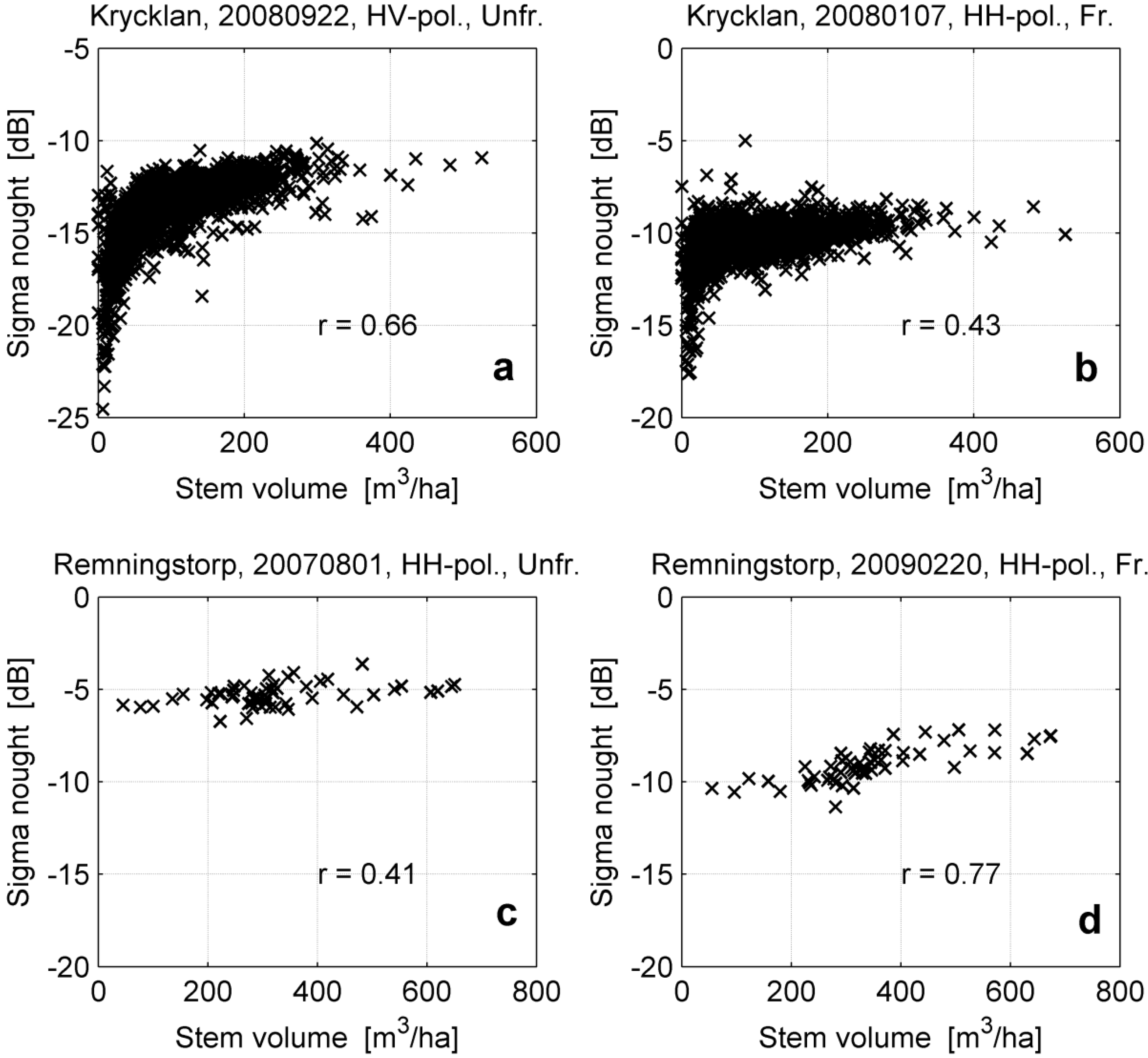
The SAR backscatter increased for increasing stem volume, with a rapid ascent for low stem volumes (<100 m³/ha or less) followed by a significant decrease of sensitivity. The relationship between the SAR backscatter and stem volume depended upon environmental conditions and polarization (see examples in Figure 3), as well as on look angle. At Krycklan, we observed strongest sensitivity of the backscatter to stem volume under unfrozen conditions and at HV-polarization (Figure 3a and Table 5). The backscatter increased rapidly for increasing stem volume; the sensitivity of the backscatter to stem volume became extremely weak in the densest forests. Observations taken during winter-time (frozen conditions or freeze/thaw events) were much less correlated with stem volume than under unfrozen conditions (Figure 3a,b and Table 5). At Remningstorp, we observed a slightly different trend, with SAR backscatter from data acquired under frozen conditions being better correlated with stem volume than in case of data acquired under unfrozen conditions (Figure 3c,d and Table 5).

An almost linear trend between SAR backscatter and stem volume was observed in several cases when images were acquired under frozen conditions. There did not seem to be any apparent difference between statistics for images acquired under unfrozen moist (i.e., <2 mm of recorded precipitation) and unfrozen wet (i.e., >2 mm of recorded precipitation) condition. Overall, the observations at the two test sites and the temporal consistency for a given environmental condition agreed with trends of the SAR backscatter at L-band with respect to stem volume and above-ground biomass in boreal as well as in other forest environments [5,6,15,16,17,18,19,20,22,23,28,39,45,46]. At both test sites, the spread of the SAR backscatter for a given stem volume was considerable, thus confirming that L-band backscatter captures only part of the information on structural properties of a forest and the signal recorded by the radar contains additional contributions [28].

Table 5. Distribution of the Pearson's correlation coefficient between stem volume and SAR backscatter for a given combination of look angle, polarization and environmental condition. Combinations are listed consisting of at least three PALSAR datasets. The minimum (Min), three quartiles (Q₁, Q₂ and Q₃) and the maximum (Max) are listed. For combinations with three datasets, only Q₂ is given. For combinations including four or five datasets, only Min, Q₂ and Max are given. Transparent cells refer to Krycklan and shaded cells to Remningstorp.

Look Angle	Polarization	Environmental Condition	Correlation Coefficient
			Min	Q1	Q2	Q3	Max
21.5°	HH	Unfrozen dry	0.14	0.17	0.25	0.32	0.39
		Unfrozen wet	0.12	0.14	0.15	0.16	0.24
	HV	Unfrozen dry	0.08	0.18	0.30	0.43	0.48
		Unfrozen wet	0.12	0.13	0.24	0.28	0.36
	VV	Unfrozen dry	0.04	0.06	0.10	0.23	0.28
		Unfrozen wet	−0.19	−0.07	0.03	0.12	0.14
34.3°	HH	Unfrozen dry	0.41	0.47	0.52	0.55	0.58
			−0.21	0.16	0.32	0.37	0.41
		Unfrozen moist	--	--	0.46	--	--
			−0.06	--	0.24	--	0.27
		Unfrozen wet	0.33	0.44	0.48	0.51	0.55
			−0.21	0.01	0.18	0.25	0.43
		Freeze	0.34	--	0.49	--	0.50
			0.09	--	0.42	--	0.63
		Frozen	0.14	0.18	0.26	0.33	0.43
			0.46	0.52	0.66	0.73	0.77
		Thaw	0.36	--	0.50	--	0.56
			--	--	0.76	--	--
	HV	Unfrozen dry	0.50	0.56	0.62	0.65	0.66
			−0.23	−0.16	−0.01	0.15	0.19
			--	--	0.01	--	--
		Unfrozen wet	0.48	0.48	0.55	0.61	0.62
			−0.26	−0.21	−0.09	0.02	0.18
41.5°	HH	Unfrozen dry	0.50	--	0.53	--	0.60
			0.36	--	0.36	--	0.36

Table 5. Distribution of the Pearson's correlation coefficient between stem volume and SAR backscatter for a given combination of look angle, polarization and environmental condition. Combinations are listed consisting of at least three PALSAR datasets. The minimum (Min), three quartiles (Q₁, Q₂ and Q₃) and the maximum (Max) are listed. For combinations with three datasets, only Q₂ is given. For combinations including four or five datasets, only Min, Q₂ and Max are given. Transparent cells refer to Krycklan and shaded cells to Remningstorp.

Look Angle	Polarization	Environmental Condition	Correlation Coefficient
			Min	Q1	Q2	Q3	Max
21.5°	HH	Unfrozen dry	0.14	0.17	0.25	0.32	0.39
		Unfrozen wet	0.12	0.14	0.15	0.16	0.24
	HV	Unfrozen dry	0.08	0.18	0.30	0.43	0.48
		Unfrozen wet	0.12	0.13	0.24	0.28	0.36
	VV	Unfrozen dry	0.04	0.06	0.10	0.23	0.28
		Unfrozen wet	−0.19	−0.07	0.03	0.12	0.14
34.3°	HH	Unfrozen dry	0.41	0.47	0.52	0.55	0.58
			−0.21	0.16	0.32	0.37	0.41
		Unfrozen moist	--	--	0.46	--	--
			−0.06	--	0.24	--	0.27
		Unfrozen wet	0.33	0.44	0.48	0.51	0.55
			−0.21	0.01	0.18	0.25	0.43
		Freeze	0.34	--	0.49	--	0.50
			0.09	--	0.42	--	0.63
		Frozen	0.14	0.18	0.26	0.33	0.43
			0.46	0.52	0.66	0.73	0.77
		Thaw	0.36	--	0.50	--	0.56
			--	--	0.76	--	--
	HV	Unfrozen dry	0.50	0.56	0.62	0.65	0.66
			−0.23	−0.16	−0.01	0.15	0.19
			--	--	0.01	--	--
		Unfrozen wet	0.48	0.48	0.55	0.61	0.62
			−0.26	−0.21	−0.09	0.02	0.18
41.5°	HH	Unfrozen dry	0.50	--	0.53	--	0.60
			0.36	--	0.36	--	0.36

Figure 3. Panels (a) and (b) illustrate data from Krycklan. Panels (c) and (d) illustrate data from Remningstorp. SAR backscatter with respect to stem volume for unfrozen (Unfr.) conditions (panels (a) and (c)) and frozen (Fr.) conditions (panels (b) and (d)) with among the highest correlation coefficients (see Table 5). Look angle: 34.3°.

Figure 3. Panels (a) and (b) illustrate data from Krycklan. Panels (c) and (d) illustrate data from Remningstorp. SAR backscatter with respect to stem volume for unfrozen (Unfr.) conditions (panels (a) and (c)) and frozen (Fr.) conditions (panels (b) and (d)) with among the highest correlation coefficients (see Table 5). Look angle: 34.3°.

5.2. Forest Backscatter Modeling

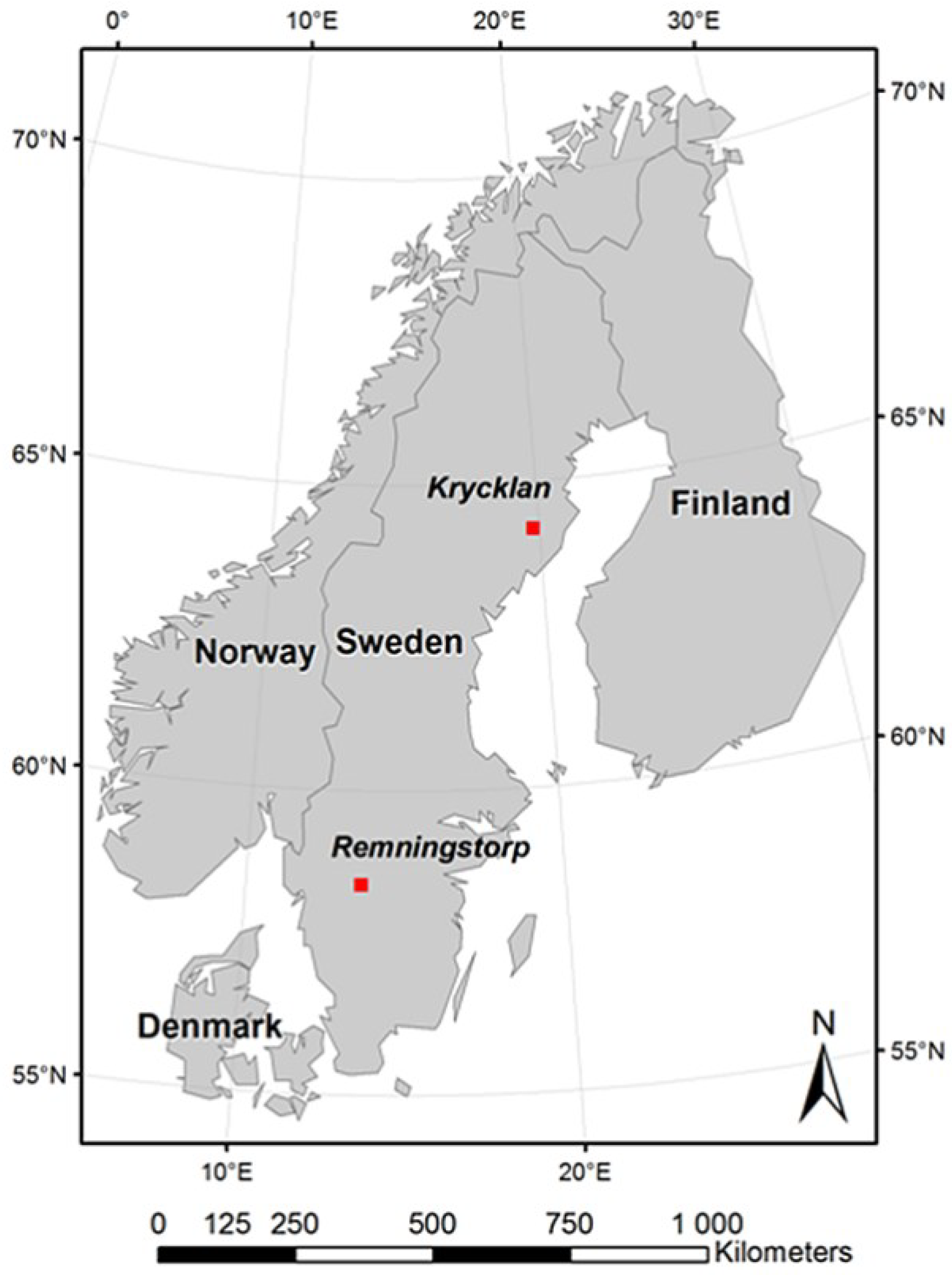
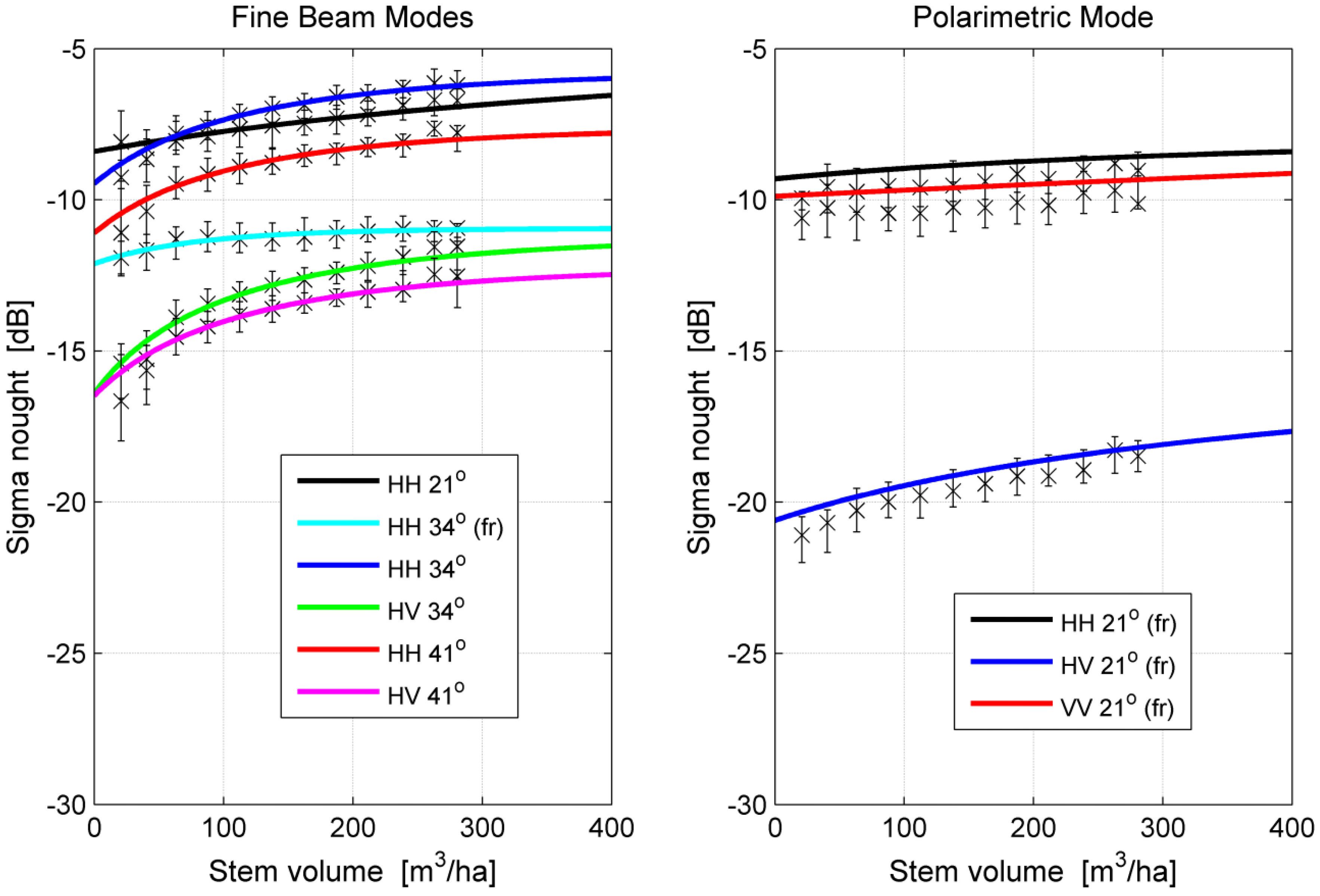
To illustrate the performance of the modeling approach with respect to the measurements of SAR backscatter and stem volume, we focus on the Krycklan test site because of the availability of stem volumes throughout all growth stages. The lack of stands with low stem volumes in Remningstorp hindered the assessment of the performance of the backscatter model in Equation (1) (as in [5]). Figure 4 shows one example of modeled and measured backscatter with respect to stem volume for each type of PALSAR dataset available at Krycklan. Taking into account previous investigation where it was shown that the backscatter is highly consistent over time for a given polarization, look angle and environmental condition [35], the examples in Figure 4 can be considered general enough to represent the behavior of the backscatter for all images available in this study. The modeled backscatter followed well the trend in the measurements (Figure 4). The strongest sensitivity of the backscatter to stem volume was found for look angles of 34.3° and 41.5° under unfrozen conditions with an increase of approximately 3 dB at HH-polarization and 4 dB at HV-polarization. Under frozen conditions, the HH-polarized backscatter increased by only 1 dB. For the 21.5° look angle, the co-polarized backscatter increased by less than 2 dB with an almost linear trend both in the FBS mode (left panel in Figure 4) and in the PLR mode (right panel in Figure 4). The HV-backscatter of the PLR mode increased by slightly less than 3 dB, thus less than the observations at shallower look angles.

Figure 4. Measured and modeled PALSAR backscatter as a function of stem volume for Krycklan. The model curves are based on Equation (1). The crosses and the vertical bars represent the median backscatter and the interquartile range in 25 m³/ha large intervals of stem volume. All data acquired under unfrozen conditions unless specified in the legend (fr = frozen).

Figure 4. Measured and modeled PALSAR backscatter as a function of stem volume for Krycklan. The model curves are based on Equation (1). The crosses and the vertical bars represent the median backscatter and the interquartile range in 25 m³/ha large intervals of stem volume. All data acquired under unfrozen conditions unless specified in the legend (fr = frozen).

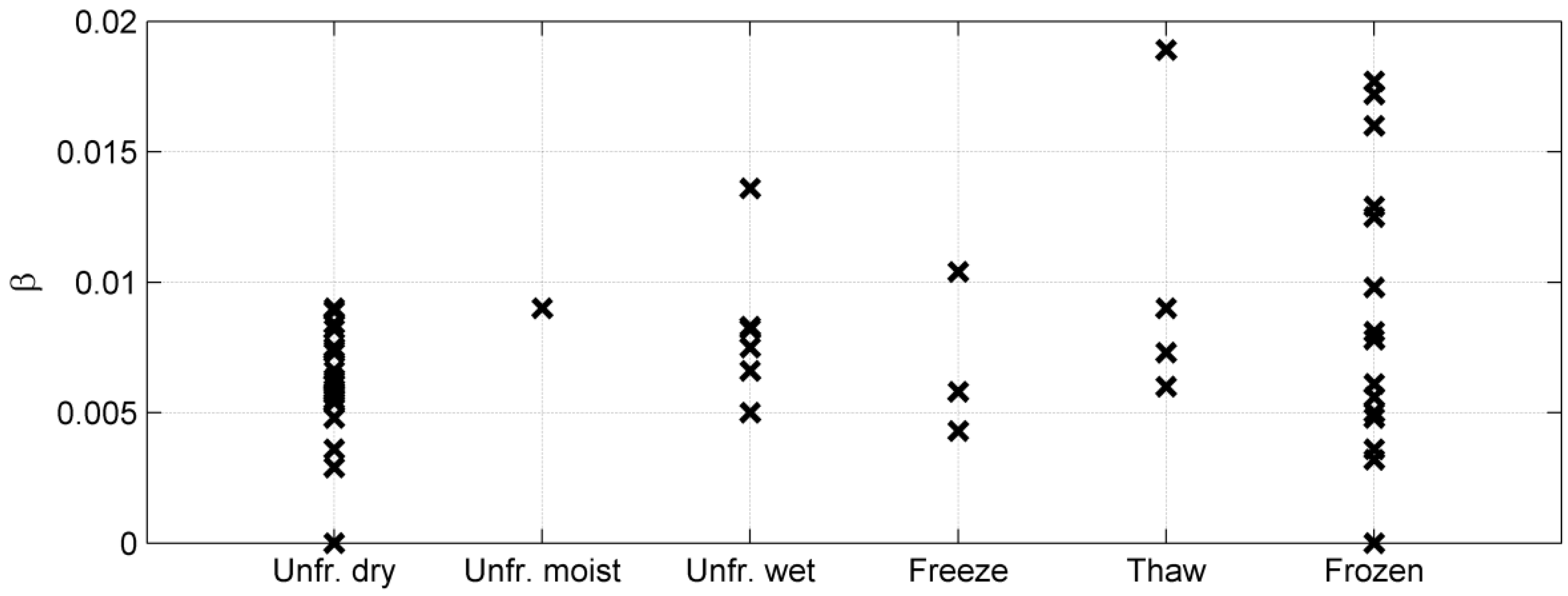
The modeled backscatter in Figure 4 was obtained by considering three unknowns in Equation (1) and showed a large range of slopes, i.e., a wide range of the values estimated for the parameter β. To get further understanding on the behavior of the coefficient β, we looked at the statistical distribution of the estimates of β with respect to environmental conditions and look angle, which was possible only for HH-polarized data. Polarization did not seem to have an effect on the estimates of the coefficient β.

To understand the dependency of β upon environmental conditions, we selected the largest dataset for a given look angle and polarization, covering all seasons (34.3° look angle and HH-polarization). The estimates of β were more consistent under unfrozen conditions than under frozen conditions or during periods of freeze/thaw transitions (Figure 5). Under unfrozen conditions, the estimates of the coefficient β were mostly between 0.005 and 0.009 (Figure 5), being in line with a previous investigation in Swedish boreal forest using JERS-1 data [5]. The estimates did not show any significant difference between dry, moist and wet environmental conditions except for one observation acquired when 12 mm of precipitation were recorded during the day. On such date, the backscatter did not show any sensitivity to the stem volume and the model curve flattened after a rapid increase for the lowest stem volumes. As a consequence, the estimate of β should not be interpreted as having a physical meaning. The same explanation applies to the observations for the case with the highest overall β estimate (0.0189), in correspondence with an acquisition under thawing conditions (temperature around the freezing point, diminishing snow cover, and precipitation). The environmental conditions affected the relationship between backscatter and stem volume to such extent that they masked out the true dependency between the two variables. Frozen conditions were characterized by the largest range of β estimates. From the weather records we could not infer dependencies between the estimates of β and weather parameters (e.g., temperature, snow depth, precipitation). We interpret the results as a consequence of the limited sensitivity of the backscatter to stem volume under frozen conditions; given the non-negligible spread of the backscatter measurements with respect to stem volume, the confidence interval of the β estimate was rather large.

Figure 5. Estimates of the model parameter β at Krycklan with respect to environmental conditions for PALSAR data acquired with 34.3° look angle and HH-polarization. “Unfr.” refers to unfrozen conditions. Frozen conditions refer to images acquired under dry conditions as well as cases with snow fall. If precipitation was recorded at <2 mm, the unfrozen conditions were moist; otherwise, the conditions were wet.

Figure 5. Estimates of the model parameter β at Krycklan with respect to environmental conditions for PALSAR data acquired with 34.3° look angle and HH-polarization. “Unfr.” refers to unfrozen conditions. Frozen conditions refer to images acquired under dry conditions as well as cases with snow fall. If precipitation was recorded at <2 mm, the unfrozen conditions were moist; otherwise, the conditions were wet.

The dependency of the estimates of β upon the look angle was limited (Figure 6). There did not seem to be any relevant difference between estimates corresponding to look angles of 34.3° and 41.5°. For both look angles, the histogram had a peak between 0.006 and 0.007. For the very few acquisitions at 21.5°, the estimates were somewhat lower (<0.004), which agrees with the understanding that at steeper look angles the forest transmissivity is higher because of larger gaps and less vegetation along the path travelled by the microwaves.

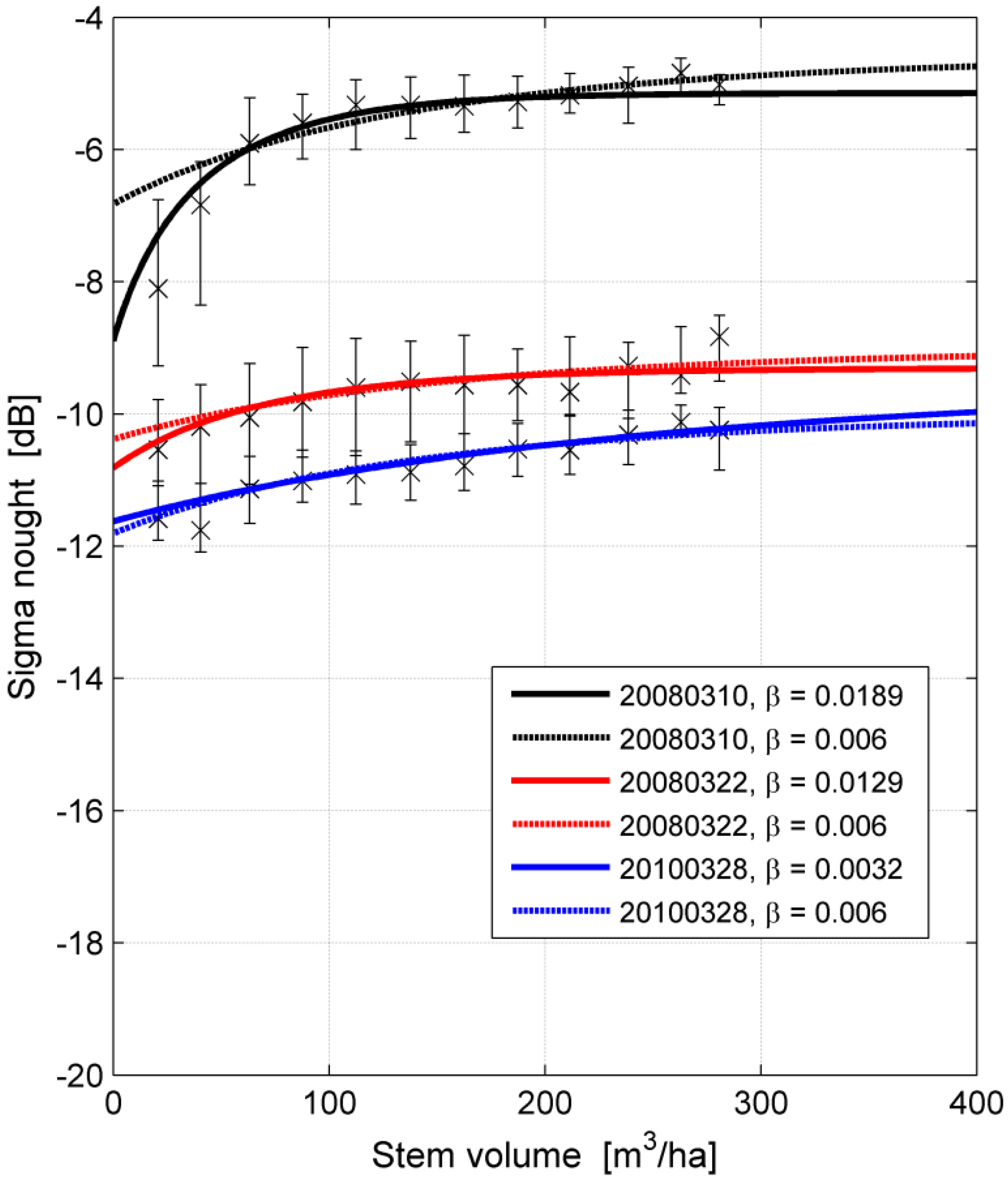
Based on the outcome of these analyses, we compared the modeled backscatter assuming β unknown a priori (i.e., model with three unknowns) and for a predefined β value (i.e., model with two unknowns). In the latter case, β was set equal to 0.006, which was considered the most reasonable value over all acquisition geometries, polarizations and environmental conditions. Figure 7 shows the modeled backscatter assuming two and three unknowns in Equation (1) for three extreme β values. The black curves correspond to the dataset for which the highest estimate of β was obtained (see Figure 7). The red and blue curves correspond to the acquisition with the highest and lowest β estimate for dry conditions, respectively; both images were acquired under frozen conditions. The modeled backscatter for such extreme cases differed only for the lowest (below 50 m³/ha) and highest (above 250 m³/ha) stem volumes. However, except for the dataset acquired under thawing conditions, the difference between the model realizations based on three and two unknowns is minimal, suggesting that a retrieval based on modeling solution where the β coefficient is set a priori equal to a constant would perform equally well as compared to a more rigorous approach where β is unknown.

Figure 6. Histograms of the estimates of the model parameter β at Krycklan as a function of look angle.

Figure 6. Histograms of the estimates of the model parameter β at Krycklan as a function of look angle.

Figure 7. Three examples of modeled backscatter as a function of stem volume assuming β unknown (solid curves) and set a priori (dashed curves). The measurements of backscatter are represented by crosses and vertical bars (median and interquartile range) for groups of stem volume, each being 25 m³/ha wide. Test site: Krycklan.

Figure 7. Three examples of modeled backscatter as a function of stem volume assuming β unknown (solid curves) and set a priori (dashed curves). The measurements of backscatter are represented by crosses and vertical bars (median and interquartile range) for groups of stem volume, each being 25 m³/ha wide. Test site: Krycklan.

5.3. Retrieval of Stem Volume

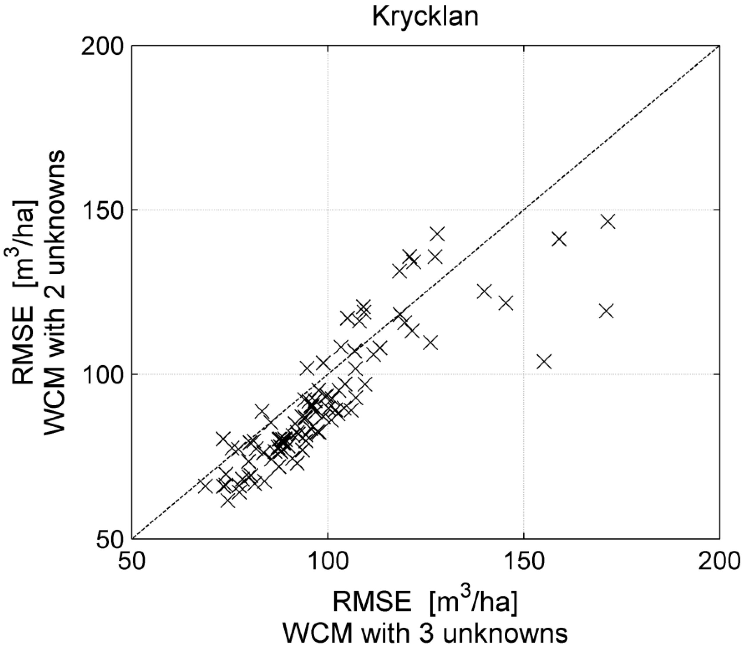
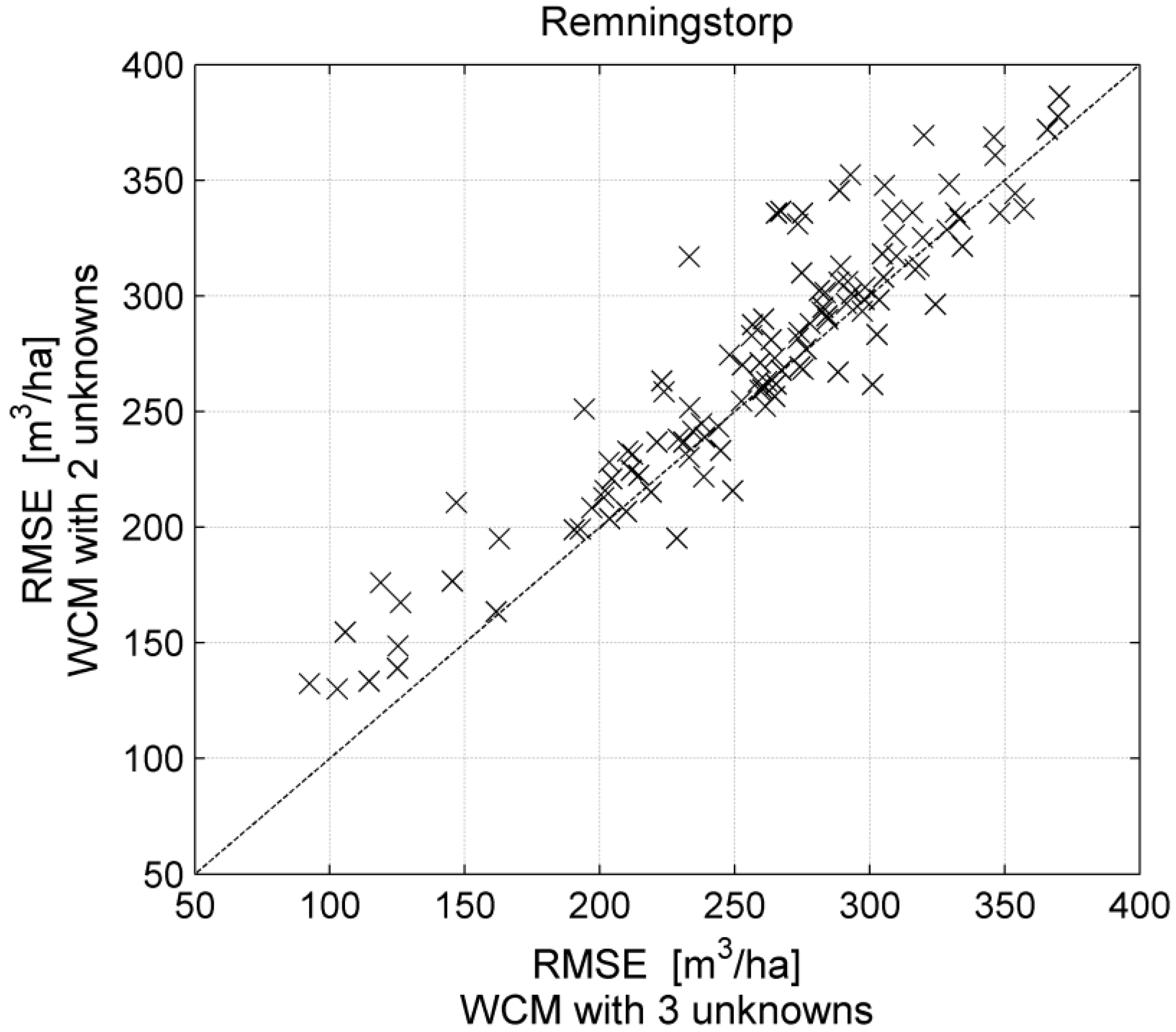
To verify that the retrieval of stem volume based on a model containing only two unknowns would perform similarly to the case of three unknowns, the RMSEs for each image acquired over Krycklan were compared (Figure 8). The scatter plot shows that the error was lower when using β = 0.006 in most cases. Only for some images acquired under frozen conditions, the model training with three unknowns performed better. Nonetheless, these images were characterized by low correlation, a consequence of the weak sensitivity of the backscatter to stem volume. At Remningstorp, the model training with a constant β = 0.006 performed in general worse than when assumed unknown a priori (Figure 9). This is a consequence of the distribution of stem volumes in the dataset available to this study. The dataset included mostly mature forest being characterized by weaker sensitivity of the backscatter to stem volume than at low stem volumes (Figure 3). The lack of stands with low stem volumes caused the estimate of the ground backscatter in the model training with two unknowns to be more imprecise and the modeled backscatter only partially fitted the observations. This effect was most prominent in images showing the highest correlation between stem volume and backscatter. It was indeed negligible for all other images where the stem volume and the backscatter were almost uncorrelated.

Figure 8. Scatter plot of single-image RMSEs for a model with three unknowns (horizontal axis) and a model with two unknowns where the parameter β was set a priori equal to 0.006 (vertical axis). Test site: Krycklan.

Figure 8. Scatter plot of single-image RMSEs for a model with three unknowns (horizontal axis) and a model with two unknowns where the parameter β was set a priori equal to 0.006 (vertical axis). Test site: Krycklan.

Figure 9. Scatter plot of single-image RMSEs for a model with three unknowns (horizontal axis) and a model with two unknowns where the parameter β was set a priori equal to 0.006 (vertical axis). Test site: Remningstorp.

Figure 9. Scatter plot of single-image RMSEs for a model with three unknowns (horizontal axis) and a model with two unknowns where the parameter β was set a priori equal to 0.006 (vertical axis). Test site: Remningstorp.

The evaluation of the retrieval is done at both test sites based on the model with two unknowns and constant β = 0.006. The RMSE for single images differed depending on polarization and environmental conditions. We evaluate the error at Krycklan in Figure 10 and Table 6; the RMSE was smaller for HV- than for HH-polarized data for similar environmental conditions. For a given polarization, slightly lower errors were obtained under unfrozen dry conditions compared to unfrozen wet and thaw conditions; much larger errors were obtained for frozen conditions (HH-polarization only) because of the much weaker sensitivity of the backscatter to stem volume (Figure 3 and Figure 4). At Remningstorp, the retrieval error was smallest under frozen conditions, at HH-polarization (see in Table 6, column of “Single-Image” retrieval for 34.3°, HH and FBS). Under unfrozen conditions, the retrieval performed poorly because of the frequent wet and moist ground conditions, which almost entirely suppressed the sensitivity of the backscatter to stem volume and caused large variability of the backscatter for similar stem volume.

The extensive dataset of PALSAR images acquired under different look angles, polarizations and environmental conditions allowed different groupings to assess the role of each on the multi-temporal combination of stem volume estimates. All retrieval statistics from the multi-temporal combination are reported in Table 6; results are grouped according to look angle and then for different combinations of polarizations. To appreciate the performance of the multi-temporal combination, the best and the worst relative RMSE for the retrieval based on a single image are also included in Table 6. Yearly retrievals have been considered to allow the multi-temporal dataset to include a fairly large number of stem volume estimates per stand while avoiding that growth and/or disturbances would distort the values of the in situ stem volumes used as reference.

Table 6. Retrieval statistics for multi-temporal combinations available in the PALSAR datasets. For each combination, the best and worst retrieval statistics for a single-image retrieval are also reported. Transparent cells refer to Krycklan and shaded cells to Remningstorp.

Look Angle	Polarization	Year	Images	Multi-Temporal Retrieval Statistics				Single-Image Rel. RMSE
				RMSE [m3/ha]	Rel. RMSE [%]	R2	Bias [m3/ha]	Best [%]	Worst [%]
21.5° (FBS)	HH	2006	2	105.2	79.2	0.14	4.9	80.6	89.8
		2006	2	217.6	68.5	0.09	−80.3	72.8	77.0
21.5° (PLR)	HH	2006	9	198.6	62.2	0.09	−1.1	70.0	110.5
		2007	3	190.7	57.2	0.09	−51.3	60.3	89.6
	HV	2006	9	173.1	54.2	0.12	−29	67.7	105.6
		2007	3	175.6	52.6	0.17	14.2	65.4	76.7
	VV	2006	9	213.4	66.9	0.02	−35.7	76.0	110.6
		2007	3	217.8	65.3	0.03	−48.6	77.8	108.2
	HH, HV, VH, VV	2006	36	176.3	55.2	0.09	−22.5	67.7	110.6
		2007	12	168.4	50.5	0.14	−16.2	59.2	108.2
34.3°	HH	2006	8	72.6	54.6	0.34	16.3	60.4	87.1
		2007	15	68.5	51.5	0.32	8.4	58.0	90.7
		2008	14	68.1	51.2	0.33	7.4	55.4	102.2
		2009	8	72.3	54.4	0.28	7.4	64.8	102.3
		2010	11	78.7	59.2	0.25	11.9	68.1	107.4
		2006	5	201.1	62.8	0.16	−0.7	62.7	92.2
		2007	11	154.3	46.4	0.34	−19.6	40.5	106.9
		2008	10	184.0	53.7	0.19	−35.9	45.3	100.9
		2009	7	121.6	35.1	0.37	−42.1	37.8	95.4
		2010	6	168.1	47.2	0.18	−54.6	49.4	97.6
	HV	2007	7	60.3	45.7	0.44	7.9	46.4	56.1
		2008	7	58.4	44.0	0.46	9.2	48.3	52.4
		2009	4	68.5	51.6	0.35	12.8	55.9	59.7
		2010	7	77.7	58.5	0.29	15.4	57.6	69.9
		2007	6	299.0	90.7	0.02	−43.7	96.5	117.2
		2008	5	268.8	78.7	0.01	−47.2	80.4	109.0
		2009	3	331.1	96.1	0.00	−27.6	96.1	96.1
		2010	4	235.7	66.2	0.00	−60.4	80.7	103.5
34.3°	HH, HV (FBD)	2007	14	60.7	45.7	0.42	7.8	46.4	67.5
		2008	14	58.8	44.2	0.44	8.5	48.3	76.7
		2009	8	68.6	51.6	0.34	12.0	55.9	70.4
		2010	14	76.1	57.3	0.29	14.6	57.6	81.5
		2007	12	237.5	72.1	0.01	−54.1	62.7	117.2
		2008	10	225.5	66.1	0.03	−53.7	61.1	109.0
		2009	6	234.5	68.1	0.01	−67.1	88.9	96.2
		2010	8	234.4	65.8	0.01	−78.5	73.9	103.5
34.3°	HH (FBS)	2007	5	77.9	58.6	0.22	13.7	66.7	90.7
		2008	10	74.3	55.9	0.28	10.1	60.4	102.2
		2009	3	93.1	70.1	0.18	−6.1	71.7	101.0
		2010	4	94.7	71.3	0.16	4.8	76.6	102.3
		2011	2	115.6	87.0	0.08	0.4	87.5	107.4
		2007	4	128.1	39.2	0.55	21.1	40.5	92.2
		2008	7	164.4	48.2	0.32	−8.7	45.3	100.8
		2009	4	171.1	48.4	0.24	−57.0	37.8	75.8
		2010	3	158.8	44.6	0.31	−21.0	49.4	54.7
	HH, HV (FBS+FBD)	2006	8	72.6	54.6	0.34	16.3	60.4	87.1
		2007	22	61.1	46.0	0.41	8.2	46.4	90.7
		2008	21	59.1	44.5	0.43	8.4	48.3	102.2
		2009	12	66.0	49.7	0.35	10.4	55.9	102.3
		2010	18	74.1	55.7	0.29	13.9	57.6	107.4
		2006	5	201.1	62.8	0.16	−0.7	62.7	92.2
		2007	17	166.8	50.2	0.21	−23.6	40.5	117.2
		2008	15	188.2	55.0	0.13	−38.6	45.3	109.0
		2009	10	120.7	35.2	0.35	−40.9	37.8	96.2
		2010	10	171.7	48.2	0.13	−56.0	49.4	103.5
41.5°	HH	2006	9	70.9	53.4	0.32	8.3	54.2	73.0
		2006	6	238.9	74.7	0.10	−24.8	74.9	86.0
	HV	2006	3	72.8	54.8	0.34	12.0	55.0	62.9
		2006	3	280.8	88.3	0.01	69.9	91.2	95.1
	HH, HV	2006	12	67.5	50.8	0.35	9.3	54.2	73.0
		2006	9	221.0	69.2	0.06	19.7	74.9	95.1
50.8°	HH	2006	2	227.2	68.9	0.21	54.5	70.8	85.8
	HH, HV	2006	4	213.1	64.6	0.23	71.2	70.6	85.8

Table 6. Retrieval statistics for multi-temporal combinations available in the PALSAR datasets. For each combination, the best and worst retrieval statistics for a single-image retrieval are also reported. Transparent cells refer to Krycklan and shaded cells to Remningstorp.

Look Angle	Polarization	Year	Images	Multi-Temporal Retrieval Statistics				Single-Image Rel. RMSE
				RMSE [m3/ha]	Rel. RMSE [%]	R2	Bias [m3/ha]	Best [%]	Worst [%]
21.5° (FBS)	HH	2006	2	105.2	79.2	0.14	4.9	80.6	89.8
		2006	2	217.6	68.5	0.09	−80.3	72.8	77.0
21.5° (PLR)	HH	2006	9	198.6	62.2	0.09	−1.1	70.0	110.5
		2007	3	190.7	57.2	0.09	−51.3	60.3	89.6
	HV	2006	9	173.1	54.2	0.12	−29	67.7	105.6
		2007	3	175.6	52.6	0.17	14.2	65.4	76.7
	VV	2006	9	213.4	66.9	0.02	−35.7	76.0	110.6
		2007	3	217.8	65.3	0.03	−48.6	77.8	108.2
	HH, HV, VH, VV	2006	36	176.3	55.2	0.09	−22.5	67.7	110.6
		2007	12	168.4	50.5	0.14	−16.2	59.2	108.2
34.3°	HH	2006	8	72.6	54.6	0.34	16.3	60.4	87.1
		2007	15	68.5	51.5	0.32	8.4	58.0	90.7
		2008	14	68.1	51.2	0.33	7.4	55.4	102.2
		2009	8	72.3	54.4	0.28	7.4	64.8	102.3
		2010	11	78.7	59.2	0.25	11.9	68.1	107.4
		2006	5	201.1	62.8	0.16	−0.7	62.7	92.2
		2007	11	154.3	46.4	0.34	−19.6	40.5	106.9
		2008	10	184.0	53.7	0.19	−35.9	45.3	100.9
		2009	7	121.6	35.1	0.37	−42.1	37.8	95.4
		2010	6	168.1	47.2	0.18	−54.6	49.4	97.6
	HV	2007	7	60.3	45.7	0.44	7.9	46.4	56.1
		2008	7	58.4	44.0	0.46	9.2	48.3	52.4
		2009	4	68.5	51.6	0.35	12.8	55.9	59.7
		2010	7	77.7	58.5	0.29	15.4	57.6	69.9
		2007	6	299.0	90.7	0.02	−43.7	96.5	117.2
		2008	5	268.8	78.7	0.01	−47.2	80.4	109.0
		2009	3	331.1	96.1	0.00	−27.6	96.1	96.1
		2010	4	235.7	66.2	0.00	−60.4	80.7	103.5
34.3°	HH, HV (FBD)	2007	14	60.7	45.7	0.42	7.8	46.4	67.5
		2008	14	58.8	44.2	0.44	8.5	48.3	76.7
		2009	8	68.6	51.6	0.34	12.0	55.9	70.4
		2010	14	76.1	57.3	0.29	14.6	57.6	81.5
		2007	12	237.5	72.1	0.01	−54.1	62.7	117.2
		2008	10	225.5	66.1	0.03	−53.7	61.1	109.0
		2009	6	234.5	68.1	0.01	−67.1	88.9	96.2
		2010	8	234.4	65.8	0.01	−78.5	73.9	103.5
34.3°	HH (FBS)	2007	5	77.9	58.6	0.22	13.7	66.7	90.7
		2008	10	74.3	55.9	0.28	10.1	60.4	102.2
		2009	3	93.1	70.1	0.18	−6.1	71.7	101.0
		2010	4	94.7	71.3	0.16	4.8	76.6	102.3
		2011	2	115.6	87.0	0.08	0.4	87.5	107.4
		2007	4	128.1	39.2	0.55	21.1	40.5	92.2
		2008	7	164.4	48.2	0.32	−8.7	45.3	100.8
		2009	4	171.1	48.4	0.24	−57.0	37.8	75.8
		2010	3	158.8	44.6	0.31	−21.0	49.4	54.7
	HH, HV (FBS+FBD)	2006	8	72.6	54.6	0.34	16.3	60.4	87.1
		2007	22	61.1	46.0	0.41	8.2	46.4	90.7
		2008	21	59.1	44.5	0.43	8.4	48.3	102.2
		2009	12	66.0	49.7	0.35	10.4	55.9	102.3
		2010	18	74.1	55.7	0.29	13.9	57.6	107.4
		2006	5	201.1	62.8	0.16	−0.7	62.7	92.2
		2007	17	166.8	50.2	0.21	−23.6	40.5	117.2
		2008	15	188.2	55.0	0.13	−38.6	45.3	109.0
		2009	10	120.7	35.2	0.35	−40.9	37.8	96.2
		2010	10	171.7	48.2	0.13	−56.0	49.4	103.5
41.5°	HH	2006	9	70.9	53.4	0.32	8.3	54.2	73.0
		2006	6	238.9	74.7	0.10	−24.8	74.9	86.0
	HV	2006	3	72.8	54.8	0.34	12.0	55.0	62.9
		2006	3	280.8	88.3	0.01	69.9	91.2	95.1
	HH, HV	2006	12	67.5	50.8	0.35	9.3	54.2	73.0
		2006	9	221.0	69.2	0.06	19.7	74.9	95.1
50.8°	HH	2006	2	227.2	68.9	0.21	54.5	70.8	85.8
	HH, HV	2006	4	213.1	64.6	0.23	71.2	70.6	85.8

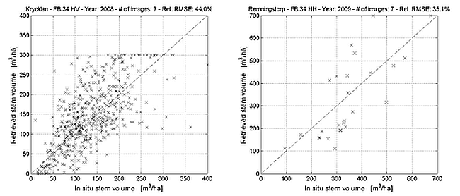
The retrieval error was never below 35%, being mostly between 40% and 70% and occasionally even in the 90% range. With respect to single-image retrieval, the stem volume estimates from the multi-temporal combination were closer to the in situ stem volumes. Table 6 shows substantial differences between the two test sites. At Krycklan, the agreement between the retrieved stem volumes with the multi-temporal combination and the in situ stem volumes was strongest for the 34.3°, HV-polarized dataset (only unfrozen conditions). The smallest relative RMSE was 44.0% from data acquired during 2008 (Table 6). Figure 11 shows that the estimated stem volume agreed well with the in situ data; nonetheless, the scatter plot did not match the 1:1 line indicating some deficiencies in either the modeling approach or the model training. 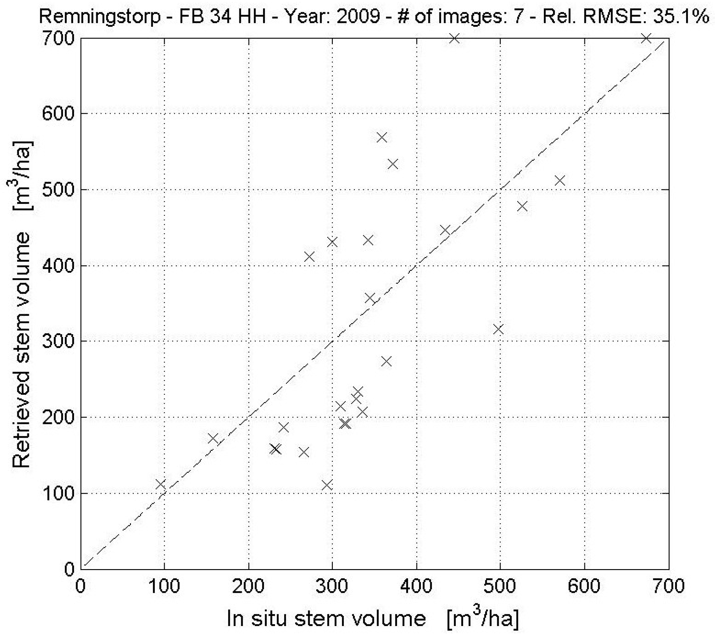The loose agreement between retrieved and in situ stem volumes is then attributed to the large scatter of the SAR backscatter for a given stem volume (see Figure 3). At Remningstorp, the best agreement between retrieved and in situ stem volumes was obtained with the 34.3°, HH-polarized dataset; the contribution of stem volumes estimated from winter-time data was predominant. The smallest relative RMSE was 35.1% from data acquired during 2009 (Table 6). As in Krycklan, the levels of retrieved and in situ stem volumes agreed well; nonetheless, the scatter between the two datasets was large (Figure 12). Remarkably, stem volume could be retrieved for the entire range of values represented at each test site (Figure 11 and Figure 12). At both test sites, the multi-temporal combination of estimates from the two polarizations of the Fine Beam modes did not perform better compared to using the best result obtained with a single polarization (i.e., HV for Krycklan and HH for Remningstorp) (Table 6). At Remningstorp, in some cases the multi-temporal retrieval using all observations performed worse compared to the best single-image retrieval or to a combination based on the couple of images characterized by the lowest RMSEs (Table 6).

Figure 10. Distribution of single-image retrieval RMSE at Krycklan for combinations of look angle, polarization and environmental conditions for which multi-temporal SAR backscatter observations (at least three) were available.

Figure 10. Distribution of single-image retrieval RMSE at Krycklan for combinations of look angle, polarization and environmental conditions for which multi-temporal SAR backscatter observations (at least three) were available.

The multi-temporal combination performed similarly across the different years, except when the RMSE was high for each of the images being combined (Table 6). In such cases, the retrieval statistics presented fluctuations, which are however of minor importance given that the retrieval performed poorly. The multi-temporal retrieval did not seem to be affected by the look angle nor could we notice an advantage of using full polarimetric data with respect to single- or dual-polarized data (Table 6). In PLR mode, the best retrieval (in a multi-temporal sense) was obtained with HV-polarized data only (Table 6); the contribution of stem volume estimates from other polarizations to the multi-temporal retrieval using all polarizations was minimal.

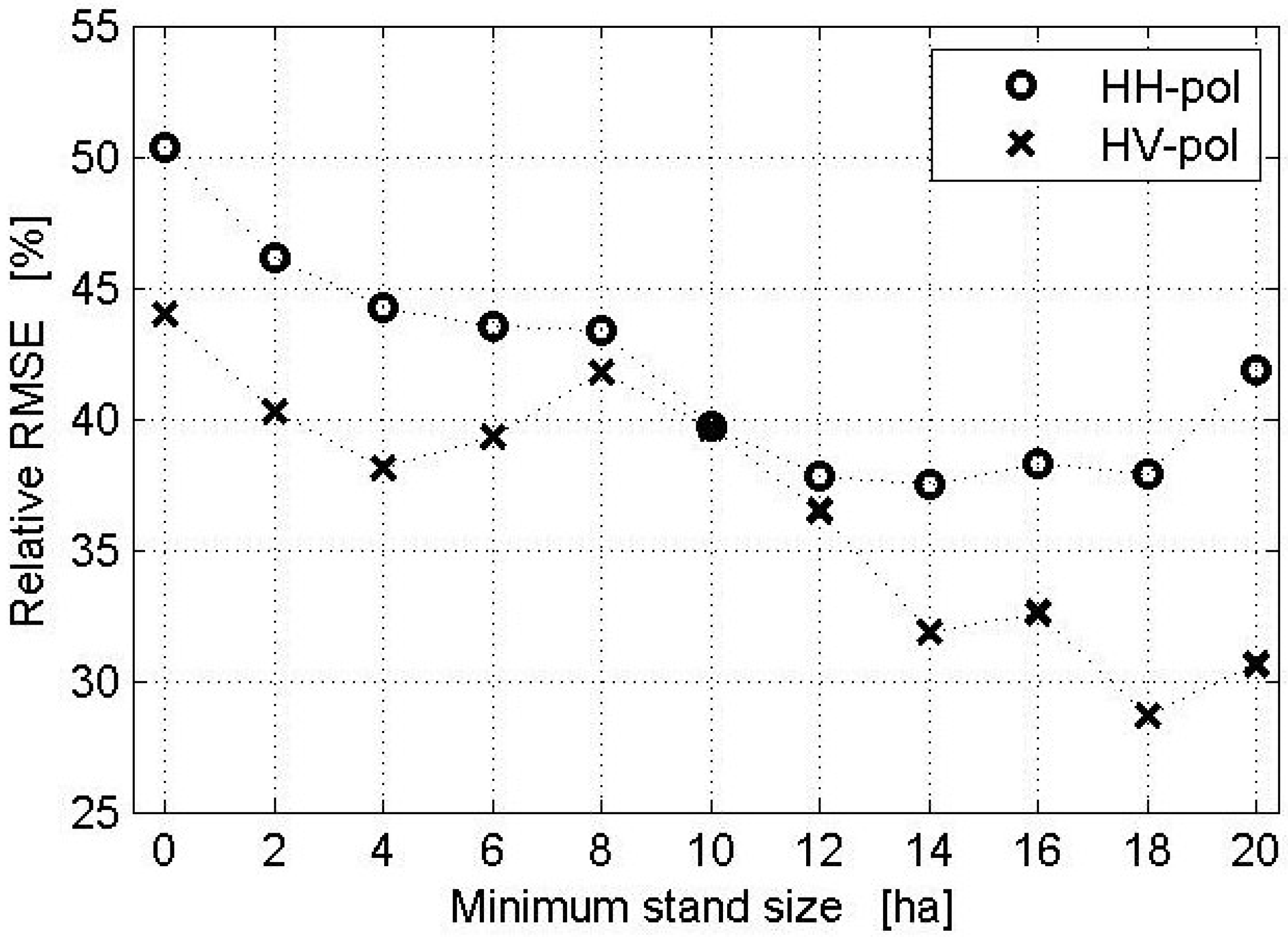
The retrieval error was finally investigated with respect to stand size. This investigation was possible at Krycklan only, because of the large range of stand sizes and number of stands (Table 1). The relative RMSE for the multi-temporal combinations of stem volumes estimated from the 34.3°, HH- and HV-polarized datasets decreased for increasing minimum stand size (Figure 13), thus confirming results in the Northeast U.S. [12]. For the retrieval based only on HV-polarized backscatter, the relative RMSE was below 30% for a minimum stand size of approximately 20 ha. The lack of a number of forest stands larger than 20 ha sufficient to compute a reliable value of the relative RMSE did not allow clarifying whether the retrieval error would further improve or reach saturation as in the case of HH-polarized data where the relative RMSE was consistently between 37% and 42% for stands with a minimum size between 10 ha and 20 ha.

Figure 11. Scatter plot of retrieved stem volume with respect to in situ stem volume in the case of all HV-polarized images acquired during 2008 over Krycklan with a look angle of 34.3°.

Figure 11. Scatter plot of retrieved stem volume with respect to in situ stem volume in the case of all HV-polarized images acquired during 2008 over Krycklan with a look angle of 34.3°.

Figure 12. Scatter plot of retrieved stem volume with respect to in situ stem volume in the case of all HH-polarized images acquired during 2009 over Remningstorp with a look angle of 34.3°.

Figure 12. Scatter plot of retrieved stem volume with respect to in situ stem volume in the case of all HH-polarized images acquired during 2009 over Remningstorp with a look angle of 34.3°.

Figure 13. Relative RMSE with respect to minimum stand size for the multi-temporal combination of stem volumes estimated from HH- and HV-polarized images acquired during 2008 over Krycklan with a look angle of 34.3°.

Figure 13. Relative RMSE with respect to minimum stand size for the multi-temporal combination of stem volumes estimated from HH- and HV-polarized images acquired during 2008 over Krycklan with a look angle of 34.3°.

6. Discussion

The extensive dataset of ALOS PALSAR images acquired over the two Swedish test sites of Krycklan (boreal forest, in the north) and Remningstorp (hemi-boreal forest, in the south) allowed a deep understanding of the relationship between stem volume and L-band backscatter observations and, in turn, on the possibility to retrieve stem volume. Taking into account that the stem volume estimates based on field measurements were updated each year with a term related to the growth factor (Section 2), we attempted to minimize the error introduced by a time lag between the acquisition of the PALSAR data and the in situ stem volume. The sensitivity of the SAR backscatter with respect to stem volume differed depending primarily on polarization and environmental conditions (Figure 3 and Table 5). Under unfrozen conditions, the L-band backscatter contrast between low and high stem volumes is affected by the forest structure and an external contribution due to soil moisture (and roughness to a certain extent). Wet conditions increase the backscatter in forest with low stem volumes while dense forests are less affected, resulting in a smaller backscatter contrast compared to unfrozen dry conditions. The effect of wet conditions is then stronger in co-polarized data than in cross-polarized data because of the surface scattering, which is negligible in the latter. For images acquired under frozen conditions, the increased transmissivity of the L-band signal through the canopy cause an increase of the ground backscatter and a decrease of the canopy backscatter resulting in an overall weaker sensitivity of the forest backscatter to stem volume. At Krycklan, the retrieval performed best under dry and unfrozen conditions, whereas frozen conditions were characterized by the largest errors (Figure 10). At Remningstorp, the frequently wet conditions under unfrozen conditions implied weak sensitivity of the backscatter to stem volume and caused the retrieval to perform poorly, regardless of the polarization. As a consequence, the frozen conditions, which implied dry terrain conditions, were characterized by the highest correlation coefficients (Table 5) and the smallest retrieval errors (Table 6).

The effect of look angle on the relationship between backscatter and stem volume was only apparent when comparing observations taken with a steep (21.5°) viewing geometry compared to a somewhat shallow (34.3° and 41.5°) look direction. For the latter, the sensitivity of the backscatter to stem volume was higher (Figure 4) as a consequence of the longer path travelled by the microwaves through the canopy, which then also implied lower retrieval errors (Table 6) for the same set of environmental conditions and polarization. This result has implications for the suitability of the data acquired in full polarimetric mode (PLR) with step look angles (i.e., <25°). The retrieval of stem volume from backscatter measurements in the PLR21 and PLR23 modes was outperformed by data acquired in FBD (and/or FBS) mode because of the shallower look angle. Even the much larger number of stem volume estimates from the PLR mode compared to the FBD or FBS mode could not compensate in the multi-temporal combination for the intrinsic limitations of the viewing geometry used when acquiring in the PLR mode.

The retrieval of stem volume was undertaken with a fairly simple but well-known modeling approach. Yet, the results showed that there are some flaws both in the model and the model training, which ultimately caused some systematic under- or overestimation of stem volume. Although the model could fit the measurements of backscatter and stem volume reasonably well for any combination of look angle, polarization and environmental conditions, the match was not always perfect (Figure 4). Given the large spread of the backscatter observations for a certain stem volume, part of the discrepancies between retrieved and in situ stem volumes could also be related to aspects not accounted for by the model. It is unclear whether such variability of the backscatter is a consequence of different forest structures or other aspects (terrain slope, soil conditions etc.). Assuming the parameter of the forest transmissivity term to be constant, the constant β = 0.006 did not seem to particularly affect the performance of the retrieval. For Remningstorp, the relative RMSE using β = 0.004 (i.e., increased transmissivity) was slightly better only in the case of winter data (32.7% vs. 35.1% for the best result using β = 0.006). Hence, it is necessary to take into account that this parameter can be spatially and temporally variable, even in a broad sense (i.e., season-dependent, forest-type dependent). For this, an evaluation of multi-temporal ALOS PALSAR datasets over different forest environments would be needed. An evaluation of other model training approaches based on non-parametric methods [22,27,47] may be worth investigating in order to provide a more comprehensive overview of the limitations of the modeling solution adopted in this study.

Overall, the multi-temporal combination improved the stem volume retrieval with respect to an estimation based on a single image. Only when the multi-temporal dataset consisted of all-but-one images with poor retrieval results, was the multi-temporal estimate characterized by a larger RMSE compared to the best single-image retrieval. Our results suggest that estimates obtained from images with the weakest sensitivity of the backscatter to stem volume (i.e., largest RMSE) should rather be neglected for the multi-temporal combination to avoid deteriorating the final stem volume estimate. The best relative RMSEs (28.1%–44.0% depending on minimum stand size at Krycklan, 35.1% at Remningstorp) are well within the range of published stem volume/biomass estimation errors for retrieval based on L-band backscatter in boreal (25% [5], 28% [6], 41%–52% [23], 63%–75% [19]), hemi-boreal (28% [20], 31%–46% [28]), sub-tropical (61% [48]), tropical savannas and woodland (48%–54% [18], 43% [17]) and tropical (20% [45]).

Looking back at the ALOS PALSAR acquisition strategy and data availability [49], the archives include the best possible datasets for the retrieval of stem volume in boreal forest. On the contrary, the retrieval in hemi-boreal forest, and in general in forest environments when the FBD data were acquired during periods of moist soils, may not perform equally well. Given the lack of similar analysis in other forest types, it is not possible to quantify the benefit of the multi-temporal observations in a more general sense. The ALOS-2 PALSAR-2 mission, started in May 2014, foresees the acquisition of dual-polarized HH and HV images during the winter season as well [49] with potential improvement of the retrieval outside of the boreal biome because of the often dry conditions. Yet it is unclear, how sensitive the HV-backscatter to stem volume is under frozen conditions given the weak attenuation of the L-band signal in the canopy and the negligible contribution of surface scattering to the cross-polarized backscatter. The increased bandwidth (28 MHz) for the dual-polarization mode shall also lead to improved estimation of stem volume given the finer scale at which data will be available. Some concern applies to the reduced availability of dense multi-temporal stacks of images, which might limit the exploitation of multi-temporal approaches to retrieve forest stem volume or above-ground biomass.

Multi-temporal observations are key to an improved stem volume retrieval accuracy with respect to a single-image retrieval, especially in the case of short wavelengths (X- and C-band) that are more affected by environmental conditions compared to L- and P-band. The major benefit of multi-temporal observations is the decrease of the retrieval error in stem volume/above-ground biomass ranges to which the sensitivity of the SAR backscatter is weak. While this approach is recommended for current spaceborne missions providing primarily data on SAR backscatter, it is likely that it will represent a simple complement in future missions specifically targeting the retrieval of forest variables (BIOMASS [50], NISAR [51], SAOCOM-CS [52]). These will prefer acquisition strategies providing observables more closely related to forest structural parameters (e.g., SAR interferometry, SAR polarimetric interferometry and SAR tomography) while the SAR backscatter will be useful for additional information, such as forest detection and forest cover change mapping.

7. Conclusions

This study looked at six years of ALOS PALSAR backscatter data (2006–2011) at two forest test sites in Sweden (Krycklan and Remningstorp) with the aim of quantifying the capability of such observations to retrieve forest stem volume. The results confirmed the rapid increase of the SAR backscatter for increasing stem volume in sparse forest (up to approximately 100 m³/ha) followed by marginal increase in high density forest. The relationship between SAR backscatter and stem volume differed depending on look angle, polarization and environmental conditions. A straightforward modeling approach based on the Water Cloud Model with gaps was able to follow reasonably well the trend in the observations; nonetheless, the retrieval was affected by the simple formulation of the model and the model training. The best retrieval results (44.0% at Krycklan using only HV-polarized data acquired under unfrozen conditions with a look angle of 34.3°; 35.1% at Remningstorp using only HH-polarized data acquired under predominantly frozen conditions with a look angle of 34.3°) indicate a reasonable performance of ALOS PALSAR backscatter to retrieve stem volume at stand level; the smaller retrieval errors for larger stands (relative RMSE <30% for stands >20 ha at Krycklan) suggests that accurate stem volume estimates are feasible at moderate resolution (pixel size >300 m) by aggregating the SAR backscatter observations from the original spatial resolution (i.e., 20–30 m) at the level of a forest stand or a moderate resolution raster.

References

1. Rosenqvist, Å.; Shimada, M.; Ito, N.; Watanabe, M. ALOS PALSAR: A pathfinder mission for global-scale monitoring of the environment. IEEE Trans. Geosci. Remote Sens. 2007, 45, 3307–3316. [Google Scholar]
2. Imhoff, M.L. Radar backscatter and biomass saturation: Ramifications for global biomass inventory. IEEE Trans. Geosci. Remote Sens. 1995, 33, 511–518. [Google Scholar] [CrossRef]
3. Ranson, K.J.; Sun, G. Mapping biomass of a northern forest using multifrequency SAR data. IEEE Trans. Geosci. Remote Sens. 1994, 32, 388–396. [Google Scholar] [CrossRef]
4. Le Toan, T.; Beaudoin, A.; Riom, J.; Guyon, D. Relating forest biomass to SAR data. IEEE Trans. Geosci. Remote Sens. 1992, 30, 403–411. [Google Scholar]
5. Santoro, M.; Eriksson, L.; Askne, J.; Schmullius, C. Assessment of stand-wise stem volume retrieval in boreal forest from JERS-1 L-band SAR backscatter. Int. J. Remote Sens. 2006, 27, 3425–3454. [Google Scholar] [CrossRef]
6. Rauste, Y. Multi-temporal JERS SAR data in boreal forest biomass mapping. Remote Sens. Environ. 2005, 97, 263–275. [Google Scholar] [CrossRef]
7. Eriksson, L.E.B.; Sandberg, G.; Ulander, L.M.H.; Smith-Jonforsen, G.; Hallberg, B.; Folkesson, K.; Fransson, J.E.S.; Magnusson, M.; Olsson, H. ALOS PALSAR calibration and validation results from Sweden. In Proceedings of the IGARSS 2007, Barcelona, Spain, 23–27 July 2007.
8. The ALOS Kyoto & Carbon Initiative, Science Plan (v.3.1). Available online: http://www.eorc.jaxa.jp/ALOS/en/kyoto/KC-Science-Plan_v3.1.pdf (accessed on 10 April 2015).
9. Andersen, H.-E.; Strunk, J.; Temesgen, H.; Atwood, D.; Winterberger, K. Using multilevel remote sensing and ground data to estimate forest biomass resources in remote regions: A case study in the boreal forests of interior Alaska. Can. J. Remote Sens. 2011, 37, 596–611. [Google Scholar] [CrossRef]
10. Santoro, M.; Askne, J.; Smith, G.; Fransson, J.E.S. Stem volume retrieval in boreal forests from ERS-1/2 interferometry. Remote Sens. Environ. 2002, 81, 19–35. [Google Scholar] [CrossRef]
11. Kurvonen, L.; Pulliainen, J.; Hallikainen, M. Retrieval of biomass in boreal forests from multitemporal ERS-1 and JERS-1 SAR images. IEEE Trans. Geosci. Remote Sens. 1999, 37, 198–205. [Google Scholar] [CrossRef]
12. Cartus, O.; Santoro, M.; Kellndorfer, J. Mapping forest aboveground biomass in the Northeastern United States with ALOS PALSAR dual-polarization L-band. Remote Sens. Environ. 2012, 124, 466–478. [Google Scholar] [CrossRef]
13. Askne, J.; Santoro, M.; Smith, G.; Fransson, J.E.S. Multitemporal repeat-pass SAR interferometry of boreal forests. IEEE Trans. Geosci. Remote Sens. 2003, 41, 1540–1550. [Google Scholar] [CrossRef]
14. Santoro, M.; Beer, C.; Cartus, O.; Schmullius, C.; Shvidenko, A.; McCallum, I.; Wegmüller, U.; Wiesmann, A. Retrieval of growing stock volume in boreal forest using hyper-temporal series of Envisat ASAR ScanSAR backscatter measurements. Remote Sens. Environ. 2011, 115, 490–507. [Google Scholar] [CrossRef]
15. Avtar, R.; Suzuki, R.; Takeuchi, W.; Sawada, H. PALSAR 50 m mosaic data based national level biomass estimation in Cambodia for implementation of REDD+ mechanism. PLoS ONE 2013, 8. [Google Scholar] [CrossRef] [PubMed]
16. Ni, W.; Sun, G.; Guo, Z.; Zhang, Z.; He, Y.; Huang, W. Retrieval of forest biomass from ALOS PALSAR data using a lookup table method. IEEE J. Sel. Top. Appl. Earth Obs. 2013, 6, 875–885. [Google Scholar] [CrossRef]
17. Mermoz, S.; le Toan, T.; Villard, L.; Réjou-Méchain, M.; Seifert-Granzin, J. Biomass assessment in the Cameroon savanna using ALOS PALSAR data. Remote Sens. Environ. 2014, 155, 109–119. [Google Scholar] [CrossRef]
18. Mitchard, E.T.A.; Saatchi, S.S.; Woodhouse, I.H.; Nangendo, G.; Ribeiro, N.S.; Williams, M.; Ryan, C.M.; Lewis, S.L.; Feldpausch, T.R.; Meir, P. Using satellite radar backscatter to predict above-ground woody biomass: A consistent relationship across four different African landscapes. Geophys. Res. Lett. 2009, 36. [Google Scholar] [CrossRef]
19. Peregon, A.; Yamagata, Y. The use of ALOS/PALSAR backscatter to estimate above-ground forest biomass: A case study in Western Siberia. Remote Sens. Environ. 2013, 137, 139–146. [Google Scholar] [CrossRef]
20. Robinson, C.; Saatchi, S.; Neumann, M.; Gillespie, T. Impacts of spatial variability on aboveground biomass estimation from L-band radar in a temperate forest. Remote Sens. 2013, 5, 1001–1023. [Google Scholar] [CrossRef]
21. Morel, A.C.; Saatchi, S.S.; Malhi, Y.; Berry, N.J.; Banin, L.; Burslem, D.; Nilus, R.; Ong, R.C. Estimating aboveground biomass in forest and oil palm plantation in Sabah, Malaysian Borneo using ALOS PALSAR data. For. Ecol. Manag. 2011, 262, 1786–1798. [Google Scholar] [CrossRef]
22. Carreiras, J.M.B.; Melo, J.B.; Vasconcelos, M.J. Estimating the above-ground biomass in miombo savanna woodlands (Mozambique, East Africa) using L-band synthetic aperture radar data. Remote Sens. 2013, 5, 1524–1548. [Google Scholar] [CrossRef]
23. Antropov, O.; Ahola, H.; Rauste, Y.; Hame, T. Stand-level stem volume of boreal forests from spaceborne SAR imagery at L-band. IEEE J. Sel. Top. Appl. Earth Obs. 2013, 6, 135–144. [Google Scholar]
24. Häme, T.; Salli, A.; Lahti, K. Estimation of carbon storage in boreal forests using remote sensing data, in Pilot study. In The Finnish Research Program on Climate Change, Progress Report; Kanninen, M., Anttila, P., Eds.; Academy of Finland: Helsinki, Finland, 1992; Volume 3, pp. 250–255. [Google Scholar]
25. Askne, J.I.A.; Fransson, J.E.S.; Santoro, M.; Soja, M.J.; Ulander, L.M.H. Model-based biomass estimation of a hemi-boreal forest from multitemporal TanDEM-X acquisitions. Remote Sens. 2013, 5, 5574–5597. [Google Scholar] [CrossRef]
26. Soja, M.J.; Sandberg, G.; Ulander, L.M.H. Regression-based retrieval of boreal forest biomass in sloping terrain using P-band SAR backscatter intensity data. IEEE Trans. Geosci. Remote Sens. 2013, 51, 2646–2665. [Google Scholar] [CrossRef]
27. Neumann, M.; Saatchi, S.S.; Ulander, L.M.H.; Fransson, J.E.S. Assessing performance of L- and P-band polarimetric interferometric SAR data in estimating boreal forest above-ground biomass. IEEE Trans. Geosci. Remote Sens. 2012, 50, 714–726. [Google Scholar] [CrossRef]
28. Sandberg, G.; Ulander, L.M.H.; Fransson, J.E.S.; Holmgren, J.; le Toan, T. L- and P-band backscatter intensity for biomass retrieval in hemiboreal forest. Remote Sens. Environ. 2011, 115, 2874–2886. [Google Scholar] [CrossRef]
29. Folkesson, K.; Smith-Jonforsen, G.; Ulander, L.M.H. Validating backscatter models for CARABAS SAR images of coniferous forests. Can. J. Remote Sens. 2008, 34, 480–495. [Google Scholar] [CrossRef]
30. Askne, J.; Santoro, M. Experiences in boreal forest stem volume estimation from multitemporal C-band InSAR. In Recent Interferometry Applications in Topography and Astronomy; Padron, I., Ed.; InTech: Morn Hill, UK, 2012. [Google Scholar]
31. Jonsson, B.; Jacobsson, J.; Kallur, H. The forest management planning package. Theory and application. Stud. For. Suec. 1993, 189, 1–56. [Google Scholar]
32. Loman, J.-O. Statistical Yearbook of Forestry 2006; Swedish Forest Agency: Jönköping, Sweden, 2006.
33. Fransson, J.E.S.; Magnusson, M.; Olsson, H.; Eriksson, L.E.B.; Sandberg, G.; Smith-Jonforsen, G.; Ulander, L.M.H. Detection of forest changes using ALOS PALSAR satellite images. In Proceedings of the IGARSS 2007, Barcelona, Spain, 23–27 July 2007.
34. Fransson, J.E.S.; Pantze, A.; Eriksson, L.E.B.; Soja, M.J.; Santoro, M. Mapping of wind-thrown forests using satellite SAR images. In Proceedings of the IGARSS 2010, Honolulu, HI, USA, 25–30 July 2010.
35. Santoro, M.; Fransson, J.E.S.; Eriksson, L.E.B.; Magnusson, M.; Ulander, L.M.H.; Olsson, H. Signatures of ALOS PALSAR L-band backscatter in Swedish forest. IEEE Trans. Geosci. Remote Sens. 2009, 47, 4001–4019. [Google Scholar] [CrossRef]
36. Wegmüller, U. Automated terrain corrected SAR geocoding. In Proceedings of the IGARSS 1999, Hamburg, Germany, 28 June–2 July 1999.
37. Shimada, M.; Isoguchi, O.; Tadono, T.; Isono, K. PALSAR radiometric and geometric calibration. IEEE Trans. Geosci. Remote Sens. 2009, 47, 3915–3932. [Google Scholar] [CrossRef]
38. Castel, T.; Beaudoin, A.; Stach, N.; Stussi, N.; le Toan, T.; Durand, P. Sensitivity of space-borne SAR data to forest parameters over sloping terrain. Theory and experiment. Int. J. Remote Sens. 2001, 22, 2351–2376. [Google Scholar] [CrossRef]
39. Fransson, J.E.S.; Israelsson, H. Estimation of stem volume in boreal forests using ERS-1 C- and JERS-1 L-band SAR data. Int. J. Remote Sens. 1999, 20, 123–137. [Google Scholar] [CrossRef]
40. Tanase, M.A.; Panciera, R.; Lowell, K.; Siyuan, T.; Garcia-Martin, A.; Walker, J.P. Sensitivity of L-band radar backscatter to forest biomass in semiarid environments: A comparative analysis of parametric and nonparametric models. IEEE Trans. Geosci. Remote Sens. 2014, 52, 4671–4685. [Google Scholar] [CrossRef]
41. Freeman, A.; Durden, S.L. A three-component scattering model for polarimetric SAR data. IEEE Trans. Geosci. Remote Sens. 1998, 36, 963–973. [Google Scholar] [CrossRef]
42. Sun, G.; Simonett, D.S.; Strahler, A.H. A radar backscatter model for discontinuous coniferous forests. IEEE Trans. Geosci. Remote Sens. 1991, 29, 639–650. [Google Scholar] [CrossRef]
43. Saatchi, S.S.; McDonald, K.C. Coherent effects in microwave backscattering models for forest canopies. IEEE Trans. Geosci. Remote Sens. 1997, 35, 1032–1044. [Google Scholar] [CrossRef]
44. Pulliainen, J.T.; Kurvonen, L.; Hallikainen, M.T. Multitemporal behavior of L- and C-band SAR observations of boreal forests. IEEE Trans. Geosci. Remote Sens. 1999, 37, 927–937. [Google Scholar] [CrossRef]
45. Saatchi, S.; Marlier, M.; Chazdon, R.; Clark, D.B.; Russell, A.E. Impact of spatial variability of tropical forest structure on radar estimation of aboveground biomass. Remote Sens. Environ. 2011, 115, 2836–2849. [Google Scholar] [CrossRef]
46. Lucas, R.; Armston, J.; Fairfax, R.; Fensham, R.; Accad, A.; Carreiras, J.; Kelley, J.; Bunting, P.; Clewley, D.; Bray, S.; et al. An evaluation of the ALOS PALSAR L-band backscatter—Above ground biomass relationship Queensland, Australia: Impacts of surface moisture condition and vegetation structure. IEEE J. Sel. Top. Appl. Earth Obs. 2010, 3, 576–593. [Google Scholar] [CrossRef]
47. Cartus, O.; Kellndorfer, J.; Walker, W.; Bishop, J.; Franco, C.; Santos, L.; Michel Fuentes, J.M. A national, detailed map of forest aboveground carbon stocks in Mexico. Remote Sens. 2014, 6, 5559–5588. [Google Scholar] [CrossRef]
48. Tanase, M.A.; Panciera, R.; Lowell, K.; Aponte, C.; Hacker, J.M.; Walker, J.P. Forest biomass estimation at high spatial resolution: Radar vs. Lidar sensors. IEEE Geosci. Remote Sens. Lett. 2013, 11, 711–715. [Google Scholar] [CrossRef]
49. Rosenqvist, A.; Shimada, M.; Suzuki, S.; Ohgushi, F.; Tadono, T.; Watanabe, M.; Tsuzuku, K.; Watanabe, T.; Kamijo, S.; Aoki, E. Operational performance of the ALOS global systematic acquisition strategy and observation plans for ALOS-2 PALSAR-2. Remote Sens. Environ. 2014, 155, 3–12. [Google Scholar] [CrossRef]
50. Le Toan, T.; Quegan, S.; Davidson, M.W.J.; Balzter, H.; Paillou, P.; Papathanassiou, K.; Plummer, S.; Rocca, F.; Saatchi, S.; Shugart, H.; et al. The BIOMASS mission: Mapping global forest biomass to better understand the terrestrial carbon cycle. Remote Sens. Environ. 2011, 115, 2850–2860. [Google Scholar] [CrossRef]
51. Rosen, P.A.; Eisen, H.; Shen, Y.; Hensley, S.; Shaffer, S.; Veilleux, L.; Dubayah, R.; Ranson, K.J.; Dress, A.; Blair, J.B.; et al. The proposed DESDynI mission—From science to implementation. In Proceedings of the IEEE Radar Conference (RADAR), Kansas City, MO, USA, 23–27 May 2011.
52. Gebert, N.; Carnicero, D.B.; Davidson, M.W.J.; Diaz, M.M.; Silvestrin, P. SAOCOM-CS—A passive companion to SAOCOM for single-pass L-band SAR interferometry. In Proceedings of the EUSAR 2014 10th European Conference on Synthetic Aperture Radar, Berlin, Germany, 3–5 June 2014.