Article

Validation and Performance Evaluations of Methods for Estimating Land Surface Temperatures from ASTER Data in the Middle Reach of the Heihe River Basin, Northwest China

1
School of Resources and Environment, University of Electronic Science and Technology of China, Chengdu 611731, China
2
State Key Laboratory of Remote Sensing Science, Research Center for Remote Sensing and GIS, and School of Geography, Beijing Normal University, Beijing 100875, China
*
Author to whom correspondence should be addressed.
Remote Sens. 2015, 7(6), 7126-7156; https://0-doi-org.brum.beds.ac.uk/10.3390/rs70607126
Submission received: 13 February 2015 / Revised: 7 May 2015 / Accepted: 22 May 2015 / Published: 29 May 2015

Abstract

:
Validation and performance evaluations are beneficial for developing methods that estimate the remotely sensed land surface temperature (LST). However, such evaluations for Advanced Spaceborne Thermal Emission and Reflection Radiometer (ASTER) data are rare. By selecting the middle reach of the Heihe River basin (HRB), China, as the study area, the atmospheric correction (AC), mono-window (MW), single-channel (SC), and split-window (SW) methods were evaluated based on in situ measured LSTs. Results demonstrate that the influences of surface heterogeneity on the validation are significant in the study area. For the AC, MW, and SC methods, the LSTs estimated from channel 13 are more accurate than those from channel 14 in general cases. When the in situ measured atmospheric profiles are available, the AC method has the highest accuracy, with a root-mean squared error (RMSE) of about 1.4–1.5 K at the homogenous oasis sites. In actual application without sufficient in situ measured inputs, the MW method is highly accurate; the RMSE is around 1.5–1.6 K. The SC method systematically overestimates LSTs and it is sensitive to error in the water vapor content. The two SW methods are simple to use but their performances are limited by accuracies, revealed by the simulation dataset. Therefore, when the in situ atmospheric profiles are available, the AC method is recommended to generate reliable ASTER LSTs for modeling the eco-hydrological processes in the middle reach of the HRB. When sufficient in situ measured inputs are not available, the MW method can be used instead.

Graphical Abstract

1. Introduction

Land surface temperature (LST) is one of the most important parameters at the interface between the earth’s surface and the atmosphere. LST acts as a sensitive indicator of climate change, and it is an essential input parameter for land surface models, e.g., Ma et al. (2015) [1]. Because of the intense variability at different spatial and temporal scales, thermal infrared (TIR) remote sensors on board satellite platforms provide the only opportunity to observe LSTs over large regions. Thus, how to estimate LSTs with the required accuracy and spatio-temporal resolutions using satellite TIR data has become an objective in the field of quantitative remote sensing over the past four decades.
The thermal radiation observed by a TIR remote sensor is attributable to the following sources: the radiation emitted by the land surface after being absorbed by the atmosphere; the radiation emitted from the atmosphere; and the atmospheric radiation reflected by the land surface after being absorbed by the atmosphere. The radiation emitted by the land surface is closely related to LST and land surface emissivity (LSE). Therefore, the LSE and atmospheric conditions are two factors that must be determined prior to estimating the LST from TIR remote sensing data. In fact, if the concurrent atmospheric profile (representing the vertical distributions of air temperature, water vapor, etc.) and the LSE were obtained when a TIR image was being acquired, it is possible to quantify the atmospheric influences with an atmospheric radiative transfer model, e.g., MODTRAN [2]. In this case, the LST can be calculated using an inversion method. However, in situ atmospheric profiles and LSEs are usually unavailable. Thus, practical methods are needed. Until now, many methods have been reported in the literature for estimating LSTs assisted by some input parameters (such as atmospheric profile, water vapor, and LSE), e.g., the single-channel method, the multi-channel method, and the multi-angle method. A comprehensive and insightful review can be found in [3].
Validation and performance evaluations of the LST methods are essential for developing valid and practical methods. In recent years, the quality of TIR data with low spatial resolutions has improved due to the demands for climate change investigations. For example, evaluations of split-window (SW) methods for estimating sea surface temperatures and LSTs from Moderate Resolution Imaging Spectroradiometer (MODIS) data are reported by [4]. Evaluations of SW methods for estimating LSTs are reported by [5] using Advanced Very High Resolution Radiometer (AVHRR), MODIS, and Visible/Infrared Imager Radiometer Suite (VIIRS) data and by [6] using Geostationary Operational Environmental Satellite (GOES) data. Evaluations of SW and temperature-emissivity separation methods are reported by [7] using MODIS data and VIIRS data. A few evaluations of the methods for TIR remote sensing data with moderate spatial resolutions have also been reported. For example, Sobrino et al. (2004) compared the atmospheric correction (AC) method, the mono-window (MW) method, and the generalized single-channel (SC) method for Landsat-5 TM data in a homogeneous plain in Spain [8]. This research found that the SC method yielded higher accuracy than the MW method. Zhou et al. (2012) evaluated four LST methods for estimating LSTs from Landsat-5 TM data in an arid region in Northwest China; they reported that these methods’ performances varied with the atmospheric conditions [9].
The Advanced Spaceborne Thermal Emission and Reflection Radiometer (ASTER), which is on board the Terra satellite that was launched in December 1999, provides TIR images with a 90-m spatial resolution in five channels over 8–12 μm [10]. Additionally, ASTER has two other subsystems that operate in the visible and near infrared (VNIR) bands with a 15-m spatial resolution and in the shortwave infrared (SWIR) band with a 30-m spatial resolution. Although images from the SWIR subsystem are not available now, ASTER still has great potential for estimating LSTs because of its multiple TIR channels. The temperature-emissivity separation method can be applied and the LST and LSE can be estimated after a preliminary atmospheric correction is conducted and after the ground-level TIR radiation is obtained [11]. The temperature-emissivity separation method is the original method for the ASTER standard LST product. In recent years, validations of this product have been reported in the literature, e.g., Wang and Liang (2009) [12]. In addition to the temperature-emissivity separation method, other methods for a single or dual TIR channel can also be applied to ASTER data. For example, Pu et al. (2006) revised the SW and MW methods for ASTER to estimate urban LSTs; these methods’ performances were evaluated qualitatively by examining the relationships between LST and the normalized difference vegetation index (NDVI) [13]. Two SW methods for AVHRR and Along-Track Scanning Radiometer (ATSR) data were adapted for ASTER by Jiménez-Muñoz and Sobrino (2007) [14]. The application of this research in agricultural areas indicated that the SW methods had an accuracy of approximately 1.5 K, which was similar to the accuracy of the ASTER standard LST product. Jiménez-Muñoz and Sobrino (2010) applied the SC method to ASTER data and compared the performances of different combinations of ASTER channels and coefficients of different training sets [15]. Their results demonstrated that the SC method had a near-zero bias and a standard deviation of approximately 2 K. Unfortunately, similar studies are rare. Additional evaluations of the performances of different methods for ASTER data are needed.
In this research, the middle reach of the Heihe River basin (HRB) in Northwest China is selected as the study area. The objective is to evaluate the performances of multiple methods for estimating LSTs from ASTER data. The results of this research will benefit the development of practical LST methods that provide input for evapotranspiration models at the field scale in agricultural areas.

2. Study Area and Datasets

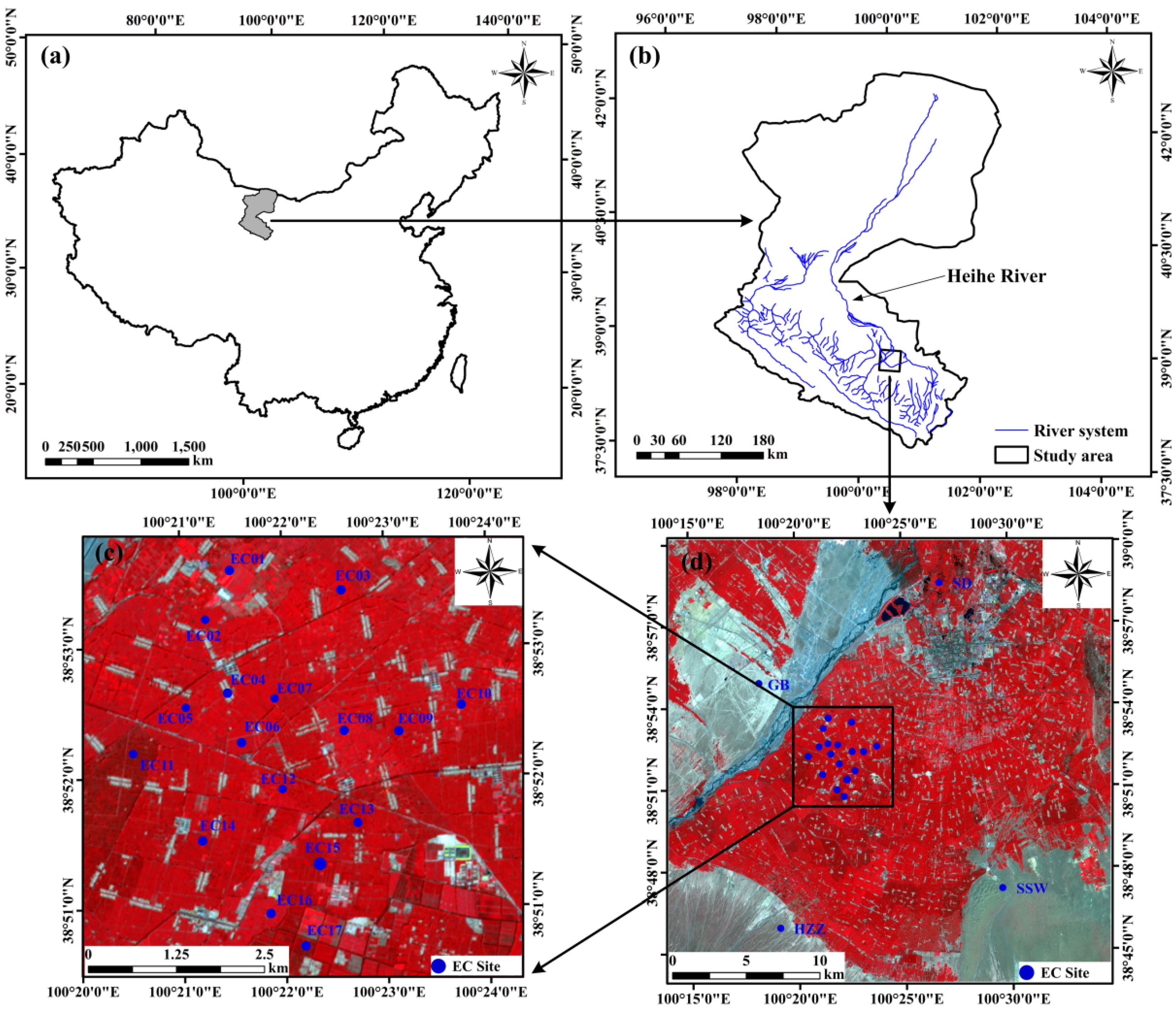
2.1. Study Area and in situ LST Measurements

The study area has an agricultural oasis-desert landscape (Figure 1). The study area’s elevation is approximately 1480 m. The climate is temperate continental, with a cold winter and a hot summer. The annual average air temperature is 7.3 °C, and the relative humidity is 52%. The annual average total precipitation is 130 mm, while the annual average evaporation is 2002 mm. The agricultural oasis benefits from the water of the Heihe River. As shown in Figure 1, the main land cover in summer is oasis cropland, residential areas, and wetland, while sandy desert, desert steppe, and the Gobi desert are common in the surrounding areas. The vegetation is dominated by corn for seed. Because of the study area’s water shortage, TIR remote sensing plays an important role in monitoring the evapotranspiration of agricultural fields in summer.
Figure 1. Map of the study area and locations of the AMSs. (a) Map of mainland China and location of the HRB; (b) map of the HRB and location of the study area; (c) locations of the AMSs within the oasis of the study area; and (d) the ASTER image (R/G/B = 3/2/1) of the study area acquired on 11 August 2012.
Remotesensing 07 07126 g001
The intensive observation period for the Heihe Watershed Allied Telemetry Experimental Research (HiWATER) program was conducted in the HRB from May to September 2012. HiWATER was designed as a comprehensive eco-hydrological experiment. Readers are encouraged to refer to Li et al. (2013) for details [16]. The in situ LST measurements, as well as other meteorological parameters, were collected by the Multi-Scale Observation Experiment on Evapotranspiration (MUSOEXE), which was the first thematic experiment of HiWATER conducted in the middle reach of the HRB [17]. There were 21 automatic meteorological stations (AMSs) in the study area, including 17 within the oasis and four outside (i.e., SSW—sandy desert, HZZ—desert steppe, GB—Gobi, and SD—wetland). All the AMSs, except for one oasis station (EC16), measured the surface incoming and outgoing shortwave radiation, the surface incoming and outgoing longwave radiation, and the net radiation with four-component radiometer sets [17,18]. The average values were provided every 10 minutes, except for the HZZ, which provided the average values every 30 minutes. Therefore, measurements from 19 AMSs were used in this research. Details on these AMSs are shown in Table 1.
Table 1. AMS stations providing the surface shortwave and longwave radiation measurements in this research.
NameFour-Component Radiometer SetLand Cover Type
InstrumentHeight (m)Diameter of FOV (m)
>EC01CNR16.044.78Vegetable
EC02CNR44.029.86Maize
EC03NR016.044.78Maize
EC04CNR16.044.78Residential areas
EC05CNR14.029.86Maize
EC06CNR46.044.78Maize
EC07CNR44.029.86Maize
EC08CNR46.044.78Maize
EC09CNR16.044.78Maize
EC10CNR16.044.78Maize
EC11CNR14.029.86Maize
EC12CNR44.029.86Maize
EC13CNR45.541.05Maize
EC14CNR46.044.78Maize
EC15PSP and PIR12.089.57Maize
EC17CNR16.044.78Apple orchard
SDNR016.044.78Wetland
GBCNR16.044.78Gobi
SSWNR016.044.78Sandy desert
Note: The CNR1 and CNR4 sets were produced by Kipp & Zonen; the PSP and PIR set was produced by the Eppley; the NR01 sets were produced by the Hukseflux.
The LST within the field of view (FOV) of the longwave pyrgeometer was calculated as follows:
T s  =  L out (1 ε b )L in ε b σ 4
where Ts is LST in K; Lout is surface outgoing longwave radiation in W·m−2; Lin is incoming longwave radiation from the atmosphere in W·m−2; εb is broadband emissivity; and σ is the Stefan–Boltzmann’s constant, which is valued at 5.67×10⁻⁸ W·m−2·K−4.
εb was calculated by weighting the component emissivities with their fractions. The component emissivities were measured with a portable 102F infrared spectrometer, with a spectral response range of 8–14 μm and a spectral resolution of 4 cm−1 [19,20,21]. The FOV of the 102F infrared spectrometer was 4.8º, and the instrument was mounted at a height of 1.1–1.2 m [20]. For each object, approximately three measurements were performed. There were in situ measured LSEs on 17 dates, and the measurements were quality checked by the provider [20]. For each ASTER image, the in situ measured LSEs on the nearest dates were used. The fractions were determined through the following two steps. First, the FOV of the longwave pyrgeometer at each site was calculated and the distributions of the internal land cover types were recorded. Second, nine photographs were taken by a digital camera every five to 10 days at each site, depending on the vegetation growth [22,23]; the component fractions of the land cover types (for example, vegetation and soil for cropland) were calculated by classifying the photographs. Because of instrument failure, in situ emissivity measurements were unavailable after 14 September 2012. Therefore, the longwave radiation values were not converted to the ground LSTs.

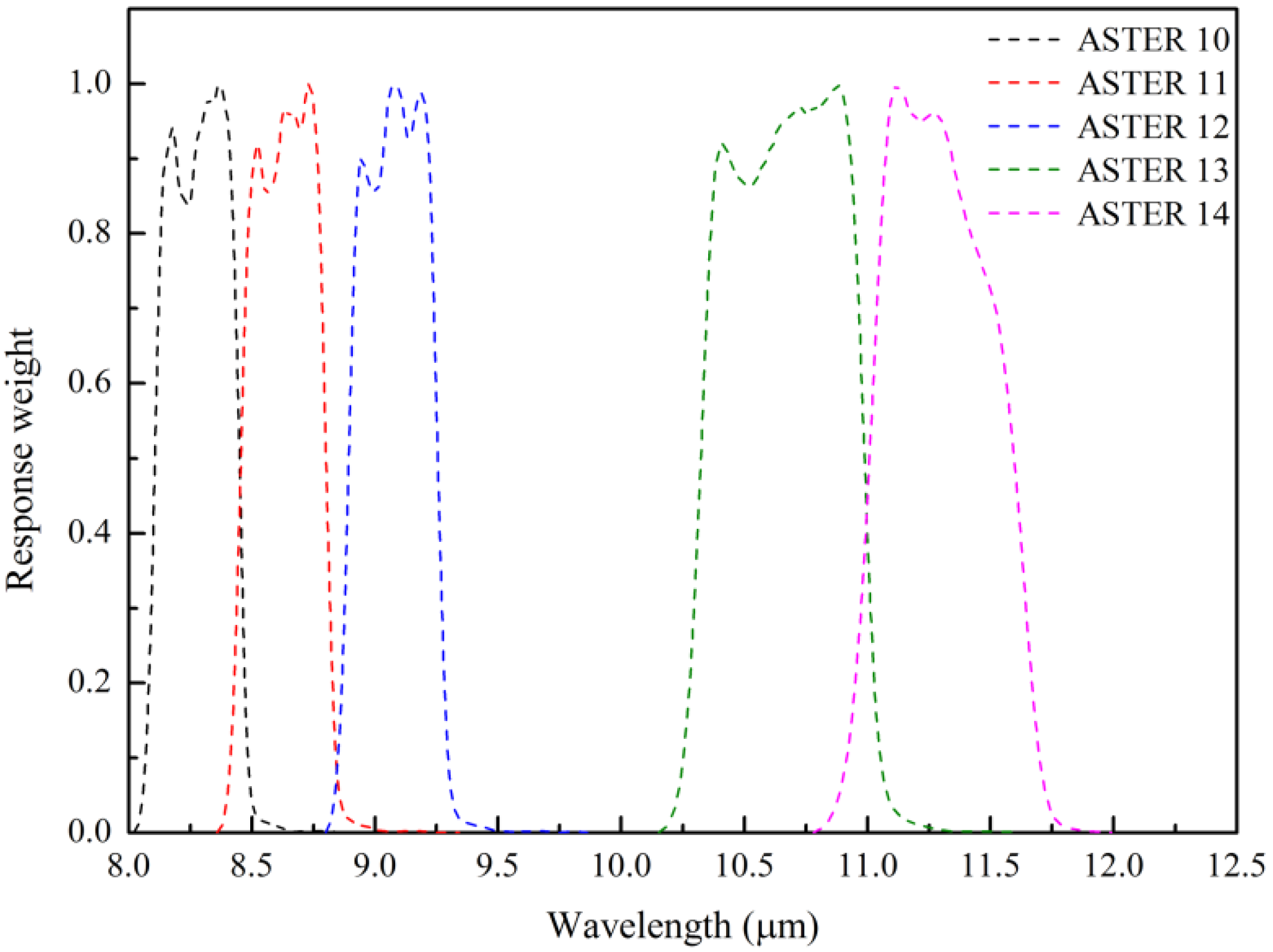
2.2. Remote Sensing Datasets

ASTER’s thermal channels have favorable specifications. The radiometric resolution is better than 0.3 K, and the absolute accuracy is better than 2 K (240–270 K) or 1 K (270–340 K) [10]. The spectral ranges of these five TIR channels are 8.125–8.475 μm, 8.475–8.825 μm, 8.925–9.275 μm, 10.25–10.95 μm, and 10.95–11.65 μm. Their spectral response functions are shown in Figure 2. Note that ASTER channels 13 and 14 have spectral ranges that are similar to the split-window channels of other satellite TIR sensors, e.g., MODIS channels 31 and 32, AVHRR channels 4 and 5, and Landsat-8 TIRS (Thermal Infrared Sensor) channels 1 and 2. Therefore, classical SW methods can also be adapted to ASTER data [24]. In addition, these two channels are also similar to the single TIR channel of Landsat TM (Thematic Mapper) and ETM+ (Enhanced Thematic Mapper Plus). Thus, the MW method and SC method may be appropriate for ASTER data.
Figure 2. Spectral response functions of the five TIR channels of ASTER.
Remotesensing 07 07126 g002
Twelve daytime ASTER images were collected under clear skies. The dates covered nearly the entire maize growing process, including the early stage in May and June (30 May, 15 June, and 24 June), the middle stage in July and August (10 July, 2 August, 11 August, 18 August, and 27 August), and the late stage in September (3, 12, 19, and 28 September). Note that the first 10 images were collected during MUSOEXE, while the last two images were collected after MUSOEXE. The overpass times for these images were approximately 04:12 to 04:19 UTC. ASTER Level-1B products (after radiometric calibration and geometric sampling), 3A01 products (orthogonal projection images), and 2B03 products (surface temperatures) were purchased from the ASTER Ground Data System of the Earth Remote Sensing Data Analysis Center of Japan.
To quantify the surface thermal heterogeneity of the study area, two airborne Thermal Airborne Spectrographic Imager (TASI) images were collected during MUSOEXE. The TASI images were acquired by the TASI-600 push-broom hyperspectral thermal sensor system between 05:37 and 10:11 UTC on 30 June 2012, and between 02:45 and 07:10 UTC on 10 July 2012 [16,25,26,27]. TASI has favorable specifications, with 32 channels in the spectral range of 8–11.5 μm [28]. The TASI images had a 3-m spatial resolution. LSTs and LSEs were estimated using a temperature-emissivity separation method, and the validations showed that the estimated LST is accurate within 1.5 K [27].

2.3. Atmospheric Profiles
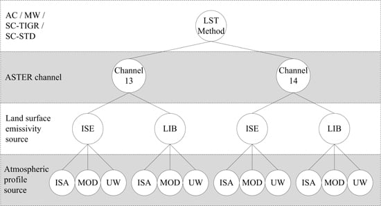
An atmospheric profile is conducive for determining the atmospheric influences in the TIR channel. Three types of atmospheric profiles were collected in this research. The first type was acquired by the Zhangye National Climate Observatory (39º05ꞌN and 100º17ꞌE) through radiosondes on the dates of the ASTER data collection [29]. This observatory is located in northern part of the study area. In June and August, the acquisition time was 05:15 UTC, which was near the overpass time of ASTER. In May and September, the acquisition time was 11:15 UTC.
The second type was extracted from the MODIS atmospheric profile products, i.e., MOD07_L2 in version 5. The MOD07_L2 profiles were selected because the product is available to the public. The spatial resolution of the MOD07_L2 product is 5 km. Compared with the in situ profiles, the MOD07_L2 products have coarser vertical resolutions, with 20 levels from 1000 hPa to 5 hPa. The overpass times of the MODIS profiles were identical to those of the ASTER images because both ASTER and MODIS are on board the Terra satellite. The third type was downloaded from the Department of Atmospheric Science at the University of Wyoming. The atmospheric profiles at 12:00 UTC at the Jiuquan station (39°46'N, 98°29'E, elevation = 1478 m) were used, and the dates of atmospheric profiles were the same as those of the ASTER images. The Jiuquan station is approximately 190 km away from our study area and has a very similar climate.

3. Methodology

3.1. Methods for Estimating LSTs

Estimating the LST from the TIR remote sensing data is based on the thermal radiance acquired by the sensor along the line of sight. Assuming that the land is a Lambertian surface in the TIR spectral range under local thermodynamic equilibrium and the sky is cloud-free, the thermal radiance acquired by the sensor can be described as follows [30]:
L i  =  ε i τ i B i ( T s ) + (1 ε i ) τ i L i  +  L i
where the subscript i denotes the channel; L is the radiance in W·m−2·μm−1·sr−1; ε is the LSE; τ is the atmospheric transmittance; B is the radiance emitted by a blackbody at temperature Ts in W·m−2·μm−1·sr−1; and L and L are the atmospheric downwelling and upwelling radiances in W·m−2·μm−1·sr−1, respectively.
Anisotropy is important factor influencing the LST estimation, but it cannot be accurately modeled in large regions at this stage. Despite the assumptions in Equation (2), studies have proven that it provides a good approximation for the radiative transfer process and that it acts as the basis for many LST methods [3]. As reviewed by [3], there are numerous LST methods. For many scientific users who are interested in applying remotely sensed LSTs in other fields (e.g., eco-hydrology and environmental science), the primary choice is a simple and practical method that has acceptable accuracy. Therefore, the following methods are examined in this research.

3.1.1. The Atmospheric Correction (AC) Method

According to Equation (2), the blackbody radiance at temperature Ts is as follows:
B i (T s ) =  L i L i (1 ε i )L i τ i ε i τ i
Then, the LST can be obtained as follows:
T s = h c λ eff k ln(1 + 2 h c 2 / λ eff 5 B i ( T s ))
where h is Planck’s constant (6.6261 × 1034 J·s); c is 299,792,458 m/s; λeff is the effective wavelength of channel i in μm; and k is Boltzmann’s constant (1.3806 × 10²³ J/K).
Apparently, the AC method requires three concurrent atmospheric parameters when the TIR image is acquired: the atmospheric transmittance, upwelling radiance, and downwelling radiance. Using the three types of atmospheric profiles in Section 2.3, these parameters were calculated for each ASTER image using the MODTRAN code in version 5.2.2.

3.1.2. The Mono-Window (MW) Method

The MW method was first proposed by Qin et al. (2001) for Landsat TM data [31]. This method relates atmospheric effects with two atmospheric parameters, i.e., the atmospheric transmittance and the effective mean atmospheric temperature. The former parameter can be estimated with the atmospheric water vapor content (WVC) based on their significant correlation. The latter parameter can be inferred from the air temperature near the surface. In the MW method, the LST is calculated as follows:
{ T s = { a i ( 1 C i D i ) + [ b i ( 1 C i D i ) + C i + D i ] T b i D i T a e f f } / C i C i = τ i ε i D i = ( 1 τ i ) [ 1 + τ i ( 1 ε i ) ]
where a and b are two coefficients that depend on the spectral response function of channel i; Tb is the at-sensor brightness temperature; and Ta-eff is the effective mean atmospheric temperature.
The MW method is appropriate for a single TIR channel. For ASTER, the atmospheric effects in channels 13 and 14 are weaker and the LSE variations are lower than those in channels 10, 11, and 12 [15]. Therefore, we applied the MW method to ASTER channels 13 and 14. Then, we fitted the coefficients a and b in Equation (5) according to the spectral response features of these two channels (Table 2).
Table 2. Coefficients a and b in the MW method for ASTER channels 13 and 14.
ChannelabR2F TestStandard Error of Estimation
130.4404−66.05060.9995128467.95110.1690
140.4620−68.83170.9996136422.04900.1720

3.1.3. The Single-Channel (SC) Method

Jiménez-Muñoz and Sobrino (2003) proposed a generalized single-channel method for estimating LSTs from a single TIR channel [32]. The most important feature of this method is that it relates atmospheric effects with three atmospheric functions of the WVC. In this method, the LST is calculated as follows:
T s  =  γ [( Ψ 1 L i + Ψ 2 )/ ε i + Ψ 3 ] +  δ
where γ and δ are two parameters related to the at-sensor brightness temperature of channel i; and ψ1, ψ2, and ψ3 are three atmospheric functions:
[ Ψ 1 Ψ 1 Ψ 1 ] = [ c 11 c 12 c 13 c 21 c 22 c 23 c 31 c 32 c 33 ] [ w 2 w 1 ]
where cij (I = 1, 2, 3; j = 1, 2, 3) can be determined based on atmospheric profiles. Jiménez-Muñoz and Sobrino (2010) used two global atmospheric profile databases to determine the coefficients in Equation (7), including TIGR61 with 61 atmospheric profiles and STD66 with 66 atmospheric profiles [15]. The TIGR61 database includes 28 tropical profiles, 12 mid-latitude summer profiles, 12 sub-arctic winter profiles, and nine U.S. Standard profiles, which were extracted from the Thermodynamic Initial Guess Retrieval (TIGR) atmospheric profile database [33,34,35]. The STD66 database was generated based on the six standard atmospheres (tropical, mid-latitude summer, mid-latitude winter, sub-arctic summer, sub-arctic winter, and U.S. Standard) included in MODTRAN code by changing the water vapor with from a scaling factor of 0.5 to 1.5 in increments of 0.1 [35]. The coefficients in Equation (7) can be found in Table 2 of [15].

3.1.4. The Split-Window (SW) Method

Split-window (SW) methods are commonly applied to the remote sensing images acquired by two adjacent TIR channels located in the atmospheric window between 10 μm and 12 μm. The basis of these methods lies in the different atmospheric absorptions of the two channels. The SW methods have different forms. A list of classical SW methods can be found in [5,24].
Jiménez-Muñoz and Sobrino (2007) adapted two SW methods intended for other TIR sensors to ASTER [14]. The first method requires WVC and LSE as inputs:
T s  =  a 0  +  a 1 ( T b i   T b j ) +  a 2 ( T b i T b j ) 2 +( a 3  +  a 4 w )(1 ε ) + ( a 5  +  a 6 w ) Δε  +  T i
where ak (k = 0, 1, …, 6) are coefficients that can be determined based on a training dataset, which is generated through comprehensive atmospheric radiative transfer simulations; ε = (εi + εj)/2; Δε = εiεj.
The second method is a simplification of Equation (8):
T s  =  a 0  +  a 1 ( T b i     T b i ) +  a 2 ( T b i T b i ) 2 T i
Equation (9) seems very simple because it relies on all parameters except for the brightness temperatures. Therefore, the method’s performance is significantly influenced by the training schemes in different atmosphere and land cover conditions. Jiménez-Muñoz and Sobrino (2007) found the two SW methods above yielded high accuracies, with root-mean squared errors (RMSEs) of 1.0 K and 1.5 K [14]. Therefore, these coefficients were utilized in our research. In this paper, the two SW methods above are abbreviated “SW-WE” and “SW-QUAD”.

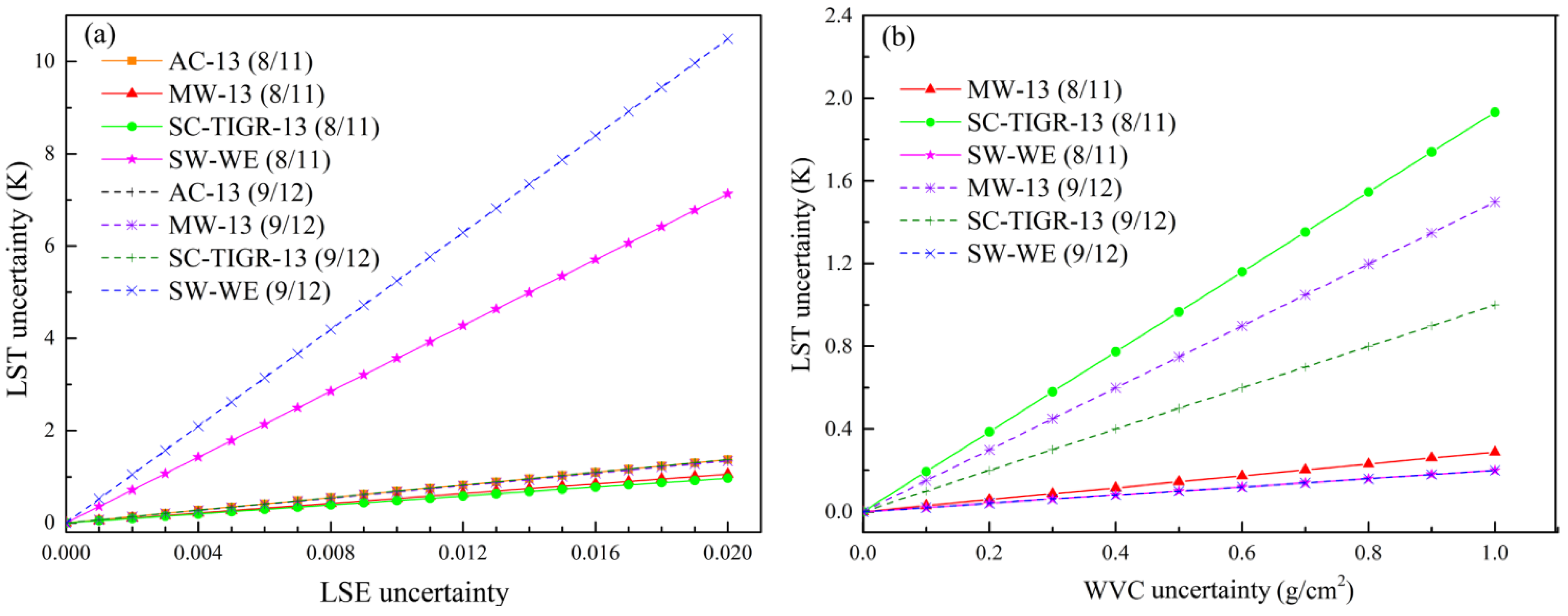
3.2. Determining the Input Parameters for Each Method

The LSE is a necessary parameter in most LST methods. In recent decades, many LSE estimation methods have been proposed for different applications [36]. One of the most frequently used practical LSE methods is the NDVI threshold (NDVITHM) method proposed by [37]. For the land surface, a pixel is treated as a mixture of soil and vegetation. This method was used here, and the required vegetation fraction was determined with the NDVI on each date. The NDVI was calculated from the land surface reflectance values of ASTER channel 3 and channel 2, which were obtained through atmospheric corrections using the in situ atmospheric profiles.
The MW method requires the input of the mean effective atmospheric temperature. We calculated this parameter based on the near-ground air temperature according to [31]. The spatially distributed near-ground air temperature was interpolated based on the air temperature measured at the AMSs. Both the MW method and SC method need WVC, which can be calculated directly from atmospheric profiles or estimated with the water vapor pressure at the ground level [9]. Using the in situ measured atmospheric profiles in this study area, a significant relationship between the water vapor pressure and WVC can therefore be calculated as follows:
w  = 0.237 e 0.0763
where e is the water vapor pressure at the ground level in hPa. There were 12 samples for training Equation (10). The coefficient of determination, R2, was 0.733.
Using the same training samples, the atmospheric transmittance in ASTER channels 13 and 14 was predicted with the WVC:
[ τ 13 τ 14 ] = [ 0.0760 0.9885 0.0921 1.0013 ] [ w 1 ]
where τ13 and τ14 are the atmospheric transmittance values in ASTER channels 13 and 14, respectively. The R2 values were 0.966 and 0.967, respectively.

3.3. Validation and Performance Evaluations of the LST Methods

Validation and performance evaluations of the LST methods were divided into two stages. First, the methods were applied to the actual ASTER dataset, and the in situ measured LSTs were used to validate the LSTs estimated with different combinations of channels and input parameters. Second, the methods were applied to the simulation dataset, and a sensitivity analysis was conducted for each method. Details can be found below.

3.3.1. The Actual ASTER Dataset

The first three methods presented in Section 3.1 can be applied to a single TIR channel, while the SW methods are applied to two TIR channels. Therefore, the AC method, the MW method, and the SC method were applied to ASTER channels 13 and 14, respectively. Note that the coefficients of the SC method for ASTER were trained using two atmospheric profile databases, i.e., STD and TIGR, as abbreviated in [14]. Thus, the SC methods with corresponding coefficients are abbreviated “SC-STD” and “SC-TIGR” in this paper. The two forms of the SW method, which used both channels 13 and 14, were considered here, i.e., SW-WE and SW-QUAD.
To evaluate the methods’ performances with LSEs from different sources, the emissivities from in situ measurements and the MODIS UCSB (University Of California Santa Barbara) Emissivity Library were selected; these two sources are denoted as ISE and LIB, respectively. The soil and vegetation emissivities required in the NDVITHM method were determined based on ISE and LIB. The water emissivity was also provided by the MODIS UCSB Emissivity Library due to the lack of in situ measurements for water.
Three sources of atmospheric profiles were also considered: the in situ measurements, MOD07_L2 profiles, and profiles from the University of Wyoming. They are abbreviated as ISA, MOD, and UW, respectively. Note that for the AC method, the atmospheric profiles were imported directly to the MODTRAN5.2.2 code; for MW, SC-STD, SC-TIGR, and SW-WE, the WVCs and atmospheric transmittance (τ) calculated based on the atmospheric profiles and estimated from the ground-level water vapor pressure were used separately. A schematic description of the various combinations is shown in Figure 3.
Figure 3. Different combinations of the LST method (AC, MW, SC-TIGR, and SC-STD), channel, LSE source, and atmospheric profile source.
Remotesensing 07 07126 g003
Eventually, there were 12, 24, 24, 24, 6, and 1 combinations for the AC, MW, SC-STD, SC-TIGR, SW-WE, and SW-QUAD methods, respectively. The LST results are recorded by the name of the method, channel, LSE source, and atmospheric profile source. For example, AC-13-ISE-ISA refers to the LST calculated with the AC method for ASTER channel 13 based on in situ measured LSE and atmospheric profiles; SW-WE-ISE-ISA refers to the LST calculated with the SW-WE method based on in situ measured LSE and WVC. In addition, the ASTER standard LST products were also processed for comparison.
A comparison between the in situ LST measurements and the remotely sensed LSTs is inevitably influenced by surface heterogeneity and scale mismatches [7,9]. However, the scale mismatches were reduced because the FOVs of the longwave pyrgeometer were comparable to the ASTER pixels. In addition, the homogeneity of the ASTER thermal pixels containing the FOVs were quantified with the TASI LSTs and ASTER NDVIs. The standard deviation of the TASI LSTs and the coefficient of variation (CV) of the ASTER NDVI at each site were calculated. The CV of the NDVI was selected as an indicator because the NDVI values were much lower for the desert and Gobi stations than for other stations. If the LST standard deviation or NDVI CV at a site exceeded the threshold, then the surface was treated as heterogeneous and removed.

3.3.2. The Simulation Dataset

Another way to evaluate LST methods is to use the simulation dataset generated by atmospheric radiative transfer models [9]. These models can simulate the at-sensor radiance acquired by a TIR channel with defined LST, LSE, and atmospheric conditions. In the simulation, atmospheric parameters such as transmittance, upwelling radiance, and downwelling radiance can be determined by the atmospheric radiative transfer model; then, LSTs can be retrieved. Thus, the accuracies of the methods can be quantified by comparing the retrieved and pre-defined LSTs.
The simulation dataset was used to evaluate each method’s performance in correcting the atmospheric effects. The simulation dataset was constructed according to the following conditions: (1) the 12 in situ measured atmospheric profiles were used as the basis data to represent the study area’s atmospheric conditions in the summer; (2) the MODTRAN code in version 5.2.2 was selected and executed in the thermal radiance mode; (3) the view zenith angle of ASTER was set to 0º; (4) the sky was clear; the rural aerosol model was used; and the visibility was defined according to the atmospheric radiosondes; (5) the LST varied between 291 K and 325 K at increments of 2 K, and the LSE varied between 0.95 and 1.0 at increments of 0.005; note that the LST and LSE ranges were determined according to the in situ measurements and the land cover types in the study area.
The simulated at-sensor spectral radiance and atmospheric parameters at every wavelength were converted to the channel-integrated values. Then, the brightness temperatures were calculated. To simulate the actual ASTER observations, random noise was added to the modeled brightness temperatures and to the at-sensor radiance. The noise for each channel was assumed to have a Gaussian distribution in the range of −0.3 K to 0.3 K, according to the ASTER noise equivalent differential temperature [38].
A sensitivity analysis was also conducted to evaluate the performance of the LST methods in overcoming the uncertainties in the input parameters. Here, the atmospheric profiles for 11 August and 12 September were selected because they were the wettest and driest dates with WVCs as of 3.11g·cm2 and 0.61 g·cm2, respectively. The LSE was defined as 0.980. The LSE uncertainty varied from 0 to 0.02 at increments of 0.001. The WVC uncertainty varied from 0 g·cm−2 to 1.0 g·cm−2 at increments of 0.1 g·cm−2. The LST uncertainty due to the WVC uncertainty in the AC, MW, SC, and SW-WE methods, and the LST uncertainty due to the LSE uncertainty in the AC, MW, and SC methods can be described as follows:
Δ T s  =  | T s ( x ) x δ x |
where ΔTs is the LST uncertainty; x and δx are the input parameter (e.g., WVC, LSEs in channel 13 or channel 14) and its uncertainty, respectively.
The LST uncertainty due to the LSE uncertainty in the SW-WE method can be described as follows:
Δ T s  =  [ T s (Δε) (Δε) δ(Δε) ] 2 + [ T s (ε) ε δε ] 2 2
where δε) and δε are the uncertainties of Δε and ε, respectively. According to [5], we assume that the LSE uncertainties in channels 13 and 14 are equal, i.e., δε13 = δε14. Therefore, δε is the same as δε13 and δε14, while δε) is 2δε.

4. Results

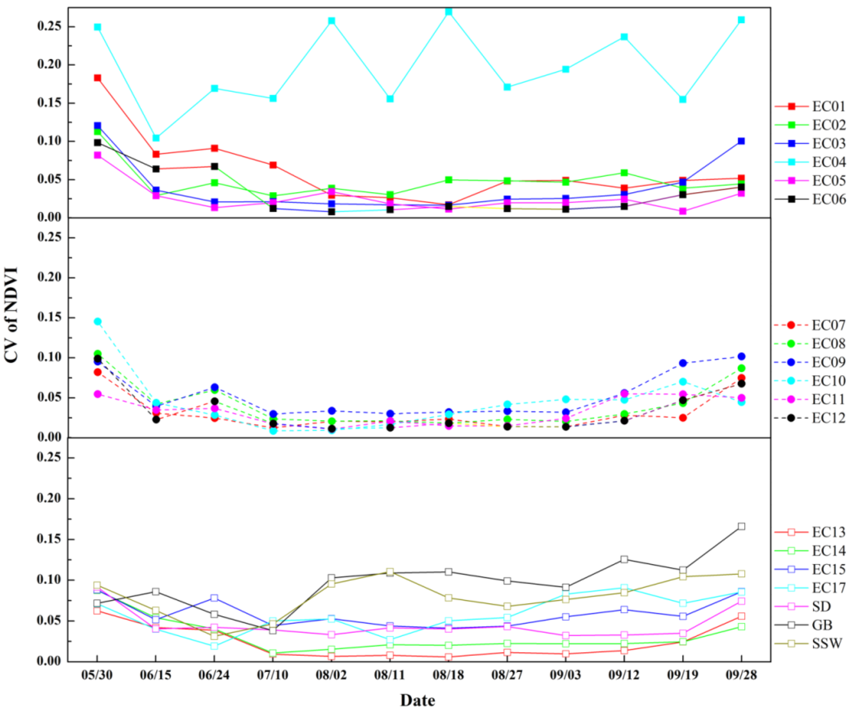
4.1. Characterizing the Surface Homogeneity of the Ground Sites

The vegetation abundance at the 19 ground sites had obvious dynamical variations, in which the vegetation increased in May and decreased in September. However, the variations in the homogeneity of these stations were different, as shown by the NDVI CV values in Figure 4. Among all the sites, EC04 had the highest NDVI CV values due to its mixed landscape of bare soil, roofs, grass, and concrete roads. The varying CV of EC04 reveals that the qualities of the calculated NDVI CV values were influenced by the atmospheric correction for the ASTER VNIR images. However, the atmospheric correction does not significantly influence the characterization of the homogeneity of the oasis sites because of their very low CV values from 15 June to 12 September, 2012. The sites had relatively higher CV values on 30 May because the crops were sprouting. As the vegetation abundance increased, the sites became more homogeneous. The heterogeneity began to increase after 12 September as the maize matured and the leaves dried out. The variation trend of the NDVI CV at EC01 was similar to those of the maize sites. However, the CV value of EC01 was higher from 30 May to 10 July because of its lower vegetation abundance during this period. The GB and SSW sites exhibited inverse variations in the NDVI CV compared with the sites located within the oasis. The heterogeneity at these two sites increased after 10 July due to their increasing vegetation abundance in the summer.
Figure 4. NDVI CV values of the 19 ground sites from 30 May to 28 September 2012.
Remotesensing 07 07126 g004
The LSTs and standard deviation values extracted from the two TASI images are shown in Figure 5. The highest standard deviation values, which exceeded 4 K on the two dates, occurred at EC04 due to the underlying mixed landscape. EC09 had standard deviation values higher than 2 K due to a wide road (approximately 4-m wide) and bare land in the FOV. EC17 had standard deviation values higher than 2 K due to the mixtures of apple trees, grasses, leguminous plants, and bare soil. The other 16 stations had low LST standard deviation values.
Here, the NDVI CV and LST standard deviation were combined to characterize the homogeneity of the underlying surface at each ground site because it was difficult to determine the thermal homogeneity on dates other than 30 June and 10 July. In fact, the selection of in situ LST measurements is a trade-off between the abundance of ground truth data and their validity. In this research, the threshold values of the NDVI CV and LST standard deviation were set to 0.08 and 2 K, respectively. After excluding the 39 heterogeneous samples from the 160 samples, 121 samples were obtained, including 110 oasis samples and 11 outside samples. The in situ measured LSTs of these samples were used to evaluate the accuracies of the methods for the actual ASTER data.
Figure 5. TASI LSTs of the 19 ground sites on 30 June and 10 July 2012. Error bars denote one time of standard deviation.
Remotesensing 07 07126 g005

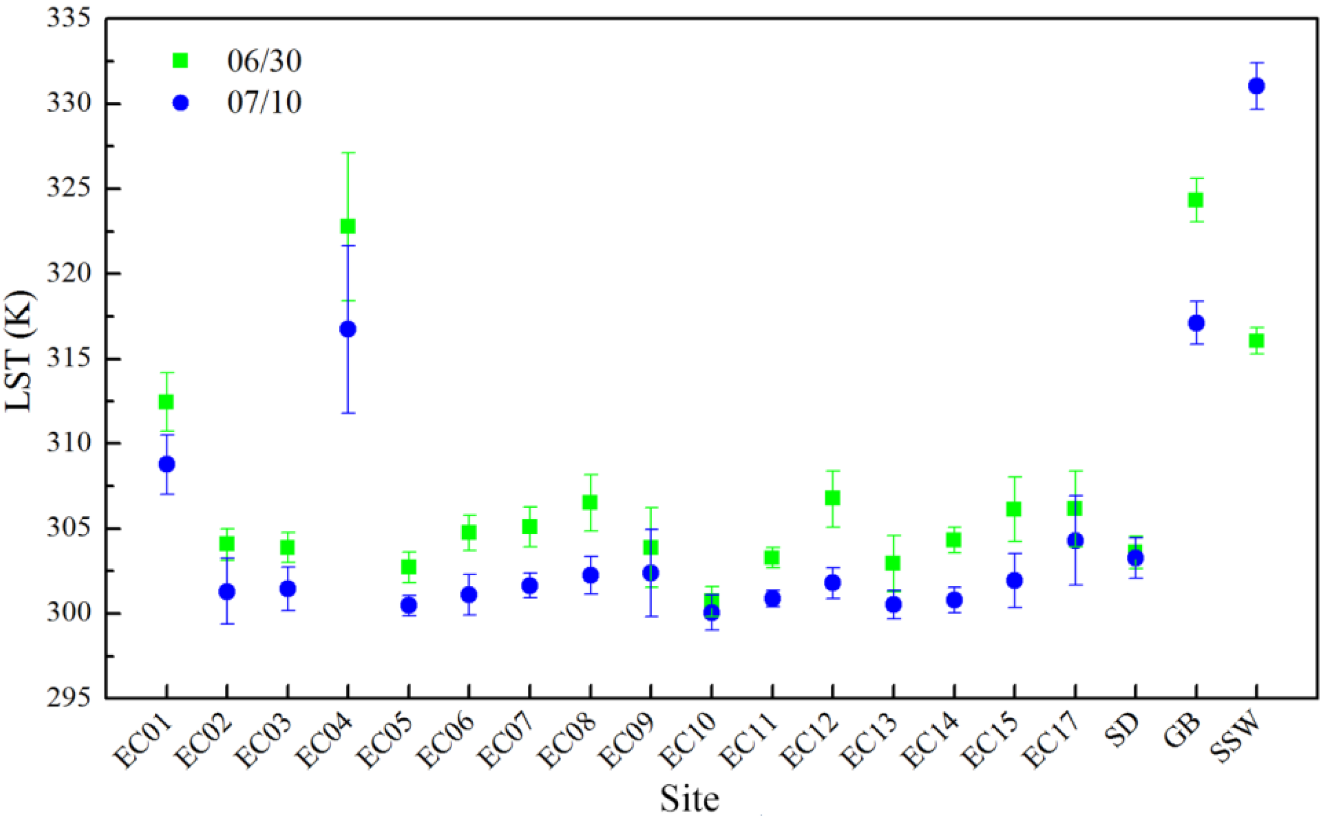
4.2. Evaluation with the in Situ Measured LSTs

LSTs of the entire study area were estimated with the methods and different combinations of LSE and atmospheric profile sources. Due to space limitations, only the LSTs resulting from AC-13-ISE-ISA are shown in Figure 6. The spatial patterns of LSTs generated through different methods and combinations were similar and they represented the actual situations in the study area. The oasis was colder than the surrounding Gobi and desert area. LSTs in both the oasis and the bare land had dynamic variations from 30 May to 28 September. These variations were induced by climatic features, meteorological conditions, and vegetation growth. Two indicators, the mean bias and RMSE, were calculated based on the in situ measured LSTs. The methods with different combinations are compared in the following sub-sections. Note that validations here are for ASTER images from 30 May to 12 September.

4.2.1. Implementing Methods with in situ Measured LSEs and Atmospheric Parameters

The biases and RMSEs of the LSTs estimated through different methods with in situ measured LSEs and atmospheric parameters are shown in Table 3. Note that the second to fourth columns are the results based on the derived WVC and τ from the atmospheric profiles directly, while the last three columns are the results based on the WVC and τ estimated from the surface meteorological observations. To demonstrate the influences of the ground sites’ heterogeneity on the validation, the biases and RMSEs calculated after removing and without removing the heterogeneous samples are both shown in Table 3. Notably, the calculated RMSEs decrease after removing these samples. Therefore, careful examinations of the in situ LST measurements are necessary before validation. An uncertainty of about 0.10–0.40 K on RMSE may result without excluding the heterogeneous samples.
Figure 6. Estimated LSTs of the study area by AC-13-ISE-ISA on the 12 dates.
Remotesensing 07 07126 g006
Table 3. Biases and RMSEs of the LSTs estimated with different methods with in situ measured LSEs and atmospheric parameters.
MethodBias and RMSE with Derived WVC and τ from the Atmospheric Profile (K)Bias and RMSE with Estimated WVC and τ (K)
Homogenous SamplesAll SamplesHomogenous SamplesAll Samples
AllOasisAllOasis
AC-13-ISE-ISA0.65 / 2.140.73 / 1.490.58 / 2.54------
AC-14-ISE-ISA0.63 / 2.210.73 / 1.550.55 / 2.65------
MW-13-ISE-ISA0.05 / 2.310.11 / 1.560.0 / 2.670.09 / 2.390.13 / 1.630.02 / 2.73
MW-14-ISE-ISA−0.06 / 2.490.03 / 1.77−0.13 / 2.880.0 / 2.570.06 / 1.84−0.10 / 2.96
SC-STD-13-ISE-ISA1.97 / 2.732.05 / 2.321.94 / 3.122.09 / 3.052.11 / 2.471.99 / 3.24
SC-STD-14-ISE-ISA2.14 / 2.892.25 / 2.512.10 / 3.292.32 / 3.352.33 / 2.762.17 / 3.52
SC-TIGR-13-ISE-ISA1.79 / 2.601.87 / 2.171.74 / 2.971.92 / 2.871.95 / 2.321.80 / 3.09
SC-TIGR-14-ISE-ISA2.06 / 2.822.17 / 2.441.99 / 3.202.24 / 3.222.27 / 2.692.08 / 3.41
SW-WE-ISE-ISA0.01 / 2.030.10 / 1.68−0.06 / 2.460.02 / 2.020.12 / 1.67−0.05 / 2.45
Using the in situ measured LSTs and atmospheric parameters as inputs, the AC method produces highly accurate results. When validated with all homogenous samples, the bias/RMSE values are 0.65 K/2.14 K and 0.63 K/2.21 K for channels 13 and 14, respectively. Therefore, the AC method seems to yield a systematic overestimation of the LST when compared with the in situ LST measurements. To the best of our knowledge, the MODTRAN code produces highly accurate results when estimating atmospheric parameters. Note that there was a one-hour gap between the overpass times and the in situ atmospheric profiles. The atmospheric influences at the atmospheric profiles acquisition time were more significant than those at the ASTER acquisition time. Therefore, overestimations of AC may result from the possible underestimations of ASTER LSEs. Compared with the AC method, except for the SW-WE method, the other methods are less accurate when using the WVC and τ directly extracted from the atmospheric profiles. In addition, most of these methods overestimate the LST. The RMSEs of the MW method are 0.17 K and 0.28 K higher than those of the AC method in channels 13 and 14, respectively. The RMSEs of the SC method are higher than those of the AC and MW methods. The SW-WE method is more accurate than the AC, MW, and SC methods. The SW-QUAD method has the best accuracy, with a bias and RMSE of 0.25 K and 1.72 K, respectively. It is reasonable to speculate that there is no influence from the uncertainty of WVC and emissivity in this method and the training conditions of the SW-QUAD method may be similar to those of the ground sites. The ASTER standard LST product has an RMSE of 2.54 K and a bias of 1.19 K. The nominal accuracy of the ASTER LST is 1.5 K, and it was proven to have a high accuracy when compared with the Surface Radiation Budget Network sites in the USA [12]. Therefore, additional evaluations of this product in other regions are needed.
With all the homogenous validating samples, the accuracies of the MW and SC methods deteriorate when using the WVC and τ estimated from the surface meteorological observations. However, the decrease in the accuracy is closely related to the method. For the MW method, the RMSE increases by 0.08 K. For the SC method, the accuracies decrease over 0.27–0.32 K and 0.40–0.46 K in channels 13 and 14, respectively. The accuracy of the SW-WE method has a negligible change. Based on Table 3, the LST estimated from channel 13 is more accurate than that from channel 14. As expected, channel 14 is more prone to significant atmospheric influences than channel 13. Therefore, a TIR channel with low atmospheric influence is the optimal choice for methods that can only be applied to a single channel.
The comparisons between estimated and measured LSTs for oasis sites are also listed in Table 3. It is interesting that all the considered methods have better accuracies when only the homogeneous oasis samples are used. For example, the RMSE values for the AC method in channels 13 and 14 decrease to 1.49 K and 1.55 K, while those for the MW method decrease to 1.56 K and 1.77 K, respectively. The SW-QUAD method still has the best accuracy, with a bias and RMSE of 0.49 K and 1.38 K, respectively. The bias and RMSE of the ASTER standard LST product decrease to 1.39 K and 2.20 K, respectively. A detailed examination of all sites’ LST errors demonstrates that the difference between validations with the homogenous oasis samples and all the homogenous samples results from poor accuracies at the SD, GB, and SSW sites. For example, significant underestimations of 2.11–8.37 K and 1.94–7.57 K on LSTs are found for the AC method applied in channel 13 and the ASTER standard LST product at the SD site. We infer that these underestimations result from the NR01 radiometer’s overestimation of the longwave radiation [17]. In addition, the mismatches between the ground site and the pixel, which is a mixture of bulrush, wet soil, and water, may contribute to these underestimations due to the geometric accuracy error. The nominal geometric accuracy error for the ASTER data is below 50 m [39]. In contrast, significant LST overestimations are found at the GB and SSW sites. The bias values at these two sites for the AC method are 1.96 K and 4.31 K, and the maximum errors are 5.32 K and 6.50 K, respectively. We believe that such overestimations result from the overestimations of atmospheric influences in the LST methods examined in this research. In implementing these methods, the atmospheric profiles and meteorological parameters within the oasis were used. Although both the GB and SSW sites are about 10 km away from the center of the oasis, their atmospheres are much drier than at the oasis sites. The average atmospheric relative humidity at the GB and SSW sites around the ASTER overpass times was about 12% and 21% lower, respectively, than at the oasis sites. An in-depth investigation on modeling the atmospheric influences is necessary if one needs accurate LSTs in the outside barren areas. Therefore, the analysis in the following sub-sections is based on the homogeneous oasis samples.

4.2.2. Implementing Methods with in Situ Measured LSEs and Alternative Atmospheric Parameters

The bias and RMSE values of every method with in situ measured LSTs and alternative atmospheric profiles are shown in Table 4. The accuracy of the AC method decreases when using the MOD and UW atmospheric profiles compared with using the in situ measured atmospheric profiles. Therefore, users should pay close attention to alternative atmospheric profiles when using the AC method. In contrast, when using the WVC and τ derived from the MOD and UW atmospheric profiles, the MW method has the same or slightly improved accuracies compared with using the in situ atmospheric profiles. From the findings of the AC method, it can be concluded that MOD and UW atmospheric profiles are not as accurate as the in situ atmospheric profiles. Therefore, the improved accuracies of the MW method may result from the compensated errors in the atmospheric profiles and the methodology; similar results are found when using the SC method and WVC and τ derived from MOD and UW atmospheric profiles. The SW-WE method has almost the same accuracy, demonstrating that it has weak sensitivity to the source of the WVC.
When using the estimated WVC and τ, the accuracy of the MW method decreases. However, the SC method is more accurate when the WVC is estimated from the MOD atmospheric profiles but less accurate when the WVC is estimated from the UW atmospheric profiles. The accuracy of the SW-WE method remains invariant. Table 4 also indicates that better accuracy is obtained in channel 13 than in channel 14.

4.2.3. Implementing Methods with Alternative LSEs and in Situ Measured Atmospheric Parameters

The biases and RMSEs of the LSTs estimated with the in situ measured atmospheric parameters and alternative LSEs are shown in Table 5. Comparing Table 3 and Table 5, no significant deterioration of the accuracies occurs for the AC, MW, and SC methods in channel 13. Therefore, when the in situ LSE measurements are unavailable in our study area, the emissivities of the MODIS UCSB Emissivity Library can be used. The accuracy of the SC method was higher for channel 14 than for channel 13. However, the RMSE is still greater than 2 K. The accuracy of the SW-WE method decreases to approximately 2.40 K when the alternative LSEs are used.
Table 4. Biases and RMSEs of the LSTs estimated with different methods with in situ measured LSEs and alternative atmospheric parameters.
MethodBias and RMSE with Derived WVC and τ from the Atmospheric Profile (K)Bias and RMSE with Estimated WVC and τ (K)
Homogenous SamplesAll SamplesHomogenous SamplesAll Samples
AllOasisAllOasis
AC-13-ISE-MOD2.18 / 3.032.24 / 2.662.14 / 3.39------
AC-14-ISE-MOD2.61 / 3.482.68 / 3.162.55 / 3.82------
MW-13-ISE-MOD0.10 / 2.290.15 / 1.460.09 / 2.68−0.11 / 2.220.0 / 1.56−0.20 / 2.57
MW-14-ISE-MOD0.02 / 2.490.09 / 1.650.0 / 2.87−0.23 / 2.39−0.10 / 1.75−0.36 / 2.77
SC-STD-13-ISE-MOD2.30 / 3.082.35 / 2.662.31 / 3.531.67 / 2.431.80 / 2.081.59 / 2.81
SC-STD-14-ISE-MOD2.60 / 3.392.67 / 3.012.63 / 3.891.77 / 2.511.93 / 2.211.67 / 2.93
SC-TIGR-13-ISE-MOD2.04 / 2.872.10 / 2.432.03 / 3.271.52 / 2.331.64 / 1.961.42 / 2.70
SC-TIGR-14-ISE-MOD2.40 / 3.202.48 / 2.822.39 / 3.621.73 / 2.491.89 / 2.171.60 / 2.86
SW-WE-ISE-MOD0.03 / 2.030.12 / 1.68-0.05 / 2.46−0.01 / 2.030.08 / 1.69−0.09 / 2.47
AC-13-ISE-UW0.95 / 2.151.06 / 1.620.87 / 2.54------
AC-14-ISE-UW1.01 / 2.221.15 / 1.710.91 / 2.64------
MW-13-ISE-UW−0.09 / 2.260.0 / 1.57−0.16 / 2.620.37 / 2.580.38 / 1.720.32 / 2.81
MW-14-ISE-UW−0.21 / 2.44−0.09 / 1.77−0.30 / 2.830.33 / 2.810.34 / 1.940.25 / 3.05
SC-STD-13-ISE-UW1.68 / 2.491.79 / 2.131.61 / 2.872.98 / 4.022.90 / 3.312.91 / 4.15
SC-STD-14-ISE-UW1.79 / 2.601.94 / 2.281.70 / 3.013.51 / 4.763.40 / 3.953.42 / 4.85
SC-TIGR-13-ISE-UW1.51 / 2.381.62 / 1.991.43 / 2.762.68 / 3.672.64 / 3.032.60 / 3.81
SC-TIGR-14-ISE-UW1.72 / 2.561.87 / 2.221.61 / 2.943.25 / 4.343.19 / 3.653.14 / 4.43
SW-WE-ISE-UW−0.02 / 2.030.07 / 1.68−0.09 / 2.460.09 / 1.990.19 / 1.660.01 / 2.43
Table 5. Biases and RMSEs of the LSTs estimated with different methods with in situ measured atmospheric parameters and alternative LSEs.
MethodBias and RMSE with Derived WVC and τ from the Atmospheric Profile (K)Bias and RMSE with Estimated WVC and τ (K)
Homogenous SamplesAll SamplesHomogenous SamplesAll Samples
AllOasisAllOasis
AC-13-LIB-ISA0.59 / 2.080.71 / 1.510.55 / 2.56------
AC-14-LIB-ISA0.13 / 2.110.25 / 1.430.08 / 2.63------
MW-13-LIB-ISA−0.01 / 2.250.09 / 1.60−0.03 / 2.690.03 / 2.330.12 / 1.66−0.02 / 2.76
MW-14-LIB-ISA−0.61 / 2.55−0.51 / 1.87−0.65 / 2.98−0.55 / 2.62−0.47 / 1.93−0.62 / 3.05
SC-STD-13-LIB-ISA1.91 / 2.652.03 / 2.321.90 / 3.112.04 / 2.962.09 / 2.471.95 / 3.22
SC-STD-14-LIB-ISA1.61 / 2.511.73 / 2.081.60 / 3.021.79 / 3.001.82 / 2.361.68 / 3.25
SC-TIGR-13-LIB-ISA1.73 / 2.521.85 / 2.171.70 / 2.961.86 / 2.791.93 / 2.331.76 / 3.08
SC-TIGR-14-LIB-ISA1.52 / 2.451.64 / 2.021.49 / 2.931.71 / 2.861.76 / 2.281.59 / 3.14
SW-WE-LIB-ISA1.62 / 2.481.81 / 2.401.48 / 2.811.61 / 2.481.80 / 2.391.47 / 2.81

4.2.4. Implementing Methods with Alternative LSEs and Atmospheric Parameters

In most real applications, both the in situ measured LSEs and atmospheric parameters are commonly unavailable. Therefore, we calculate the biases and RMSEs of the LSTs estimated with different methods with alternative LSEs and atmospheric parameters. The results are shown in Table 6. The biases and RMSEs of the AC method demonstrate that similar accuracies can be obtained when the library LSEs are used. An even better accuracy is achieved with channel 14. The MW method does not provide significant systematic estimations at the ground sites, particularly in channel 13. In channel 13, the RMSE varies from 1.49 K and 1.60 K when the WVC and τ are derived directly from MOD and UW atmospheric profiles and from 1.58 K and 1.74 K when the estimated WVC and τ are used. The accuracies of the MW method are lower in channel 14 than in channel 13 because the MW method is less able to remove the atmospheric influences in channel 14.
Table 6. Biases and RMSEs of the LSTs estimated with different methods with alternative LSEs and atmospheric parameters.
MethodBias and RMSE with Derived WVC and τ from the Atmospheric Profile (K)Bias and RMSE with Estimated WVC and τ (K)
Homogenous SamplesAll SamplesHomogenous SamplesAll Samples
AllOasisAllOasis
AC-13-LIB-MOD2.13 / 2.952.23 / 2.652.10 / 3.35------
AC-14-LIB-MOD2.09 / 3.122.18 / 2.772.07 / 3.53------
MW-13-LIB-MOD0.04 / 2.220.13 / 1.490.06 / 2.67−0.16 / 2.18−0.02 / 1.58−0.24 / 2.60
MW-14-LIB-MOD−0.52 / 2.52−0.44 / 1.73−0.50 / 2.93−0.79 / 2.50−0.64 / 1.89−0.89 / 2.91
SC-STD-13-LIB-MOD2.24 / 3.002.33 / 2.662.28 / 3.491.62 / 2.361.78 / 2.081.55 / 2.80
SC-STD-14-LIB-MOD2.07 / 3.002.16 / 2.602.14 / 3.591.23 / 2.151.41 / 1.781.17 / 2.69
SC-TIGR-13-LIB-MOD1.99 / 2.792.08 / 2.432.00 / 3.241.47 / 2.261.63 / 1.961.38 / 2.69
SC-TIGR-14-LIB-MOD1.87 / 2.831.96 / 2.401.89 / 3.321.18 / 2.131.35 / 1.751.09 / 2.63
SW-WE-LIB-MOD1.61 / 2.471.80 / 2.391.47 / 2.801.64 / 2.491.83 / 2.411.50 / 2.81
AC-13-LIB-UW0.90 / 2.091.04 / 1.630.83 / 2.55------
AC-14-LIB-UW0.49 / 2.040.64 / 1.470.42 / 2.55------
MW-13-LIB-UW−0.15 / 2.21−0.02 / 1.60−0.20 / 2.650.32 / 2.500.36 / 1.740.28 / 2.81
MW-14-LIB-UW−0.77 / 2.55−0.63 / 1.91−0.83 / 2.96−0.20 / 2.78−0.18 / 1.96−0.25 / 3.07
SC-STD-13-LIB-UW1.62 / 2.421.77 / 2.131.57 / 2.872.93 / 3.932.89 / 3.312.88 / 4.10
SC-STD-14-LIB-UW1.24 / 2.261.41 / 1.871.19 / 2.773.02 / 4.392.93 / 3.562.96 / 4.52
SC-TIGR-13-LIB-UW1.45 / 2.311.60 / 1.991.39 / 2.762.63 / 3.582.62 / 3.022.57 / 3.76
SC-TIGR-14-LIB-UW1.16 / 2.221.32 / 1.821.09 / 2.722.75 / 3.962.70 / 3.262.67 / 4.11
SW-WE-LIB-UW1.65 / 2.501.83 / 2.421.50 / 2.821.56 / 2.451.75 / 2.361.42 / 2.79
The SC method has significant systematic overestimations at the ground sites when using the alternative LSEs and atmospheric parameters. Higher accuracies are obtained when the WVC and τ of the UW atmospheric profiles are used than when the MOD atmospheric profiles are used. However, when the estimated WVC and τ are used, higher accuracies are obtained with the MOD atmospheric profiles. In this case, the RMSEs in channel 14 are approximately 0.2~0.3 K higher than those in channel 13. Generally, higher accuracies appear when the coefficients trained by the TIGR atmospheric profile database are used. Therefore, the coefficients trained by the TIGR atmospheric profile database are more appropriate for our study area than those trained by the STD atmospheric profile database. The RMSEs of the SW-WE method using alternative LSEs and atmospheric parameters are approximately 2.40 K. Comparing Table 4 and Table 6, it is obvious that the low accuracy of the SW-WE method may result from the LIB LSEs. Among all the LSE and atmospheric profile combinations, MW-13-LIB-MOD and AC-14-LIB-UW have the highest accuracies, with corresponding biases/RMSEs of 0.13 K/1.49 K and 0.64 K/1.47 K, respectively.

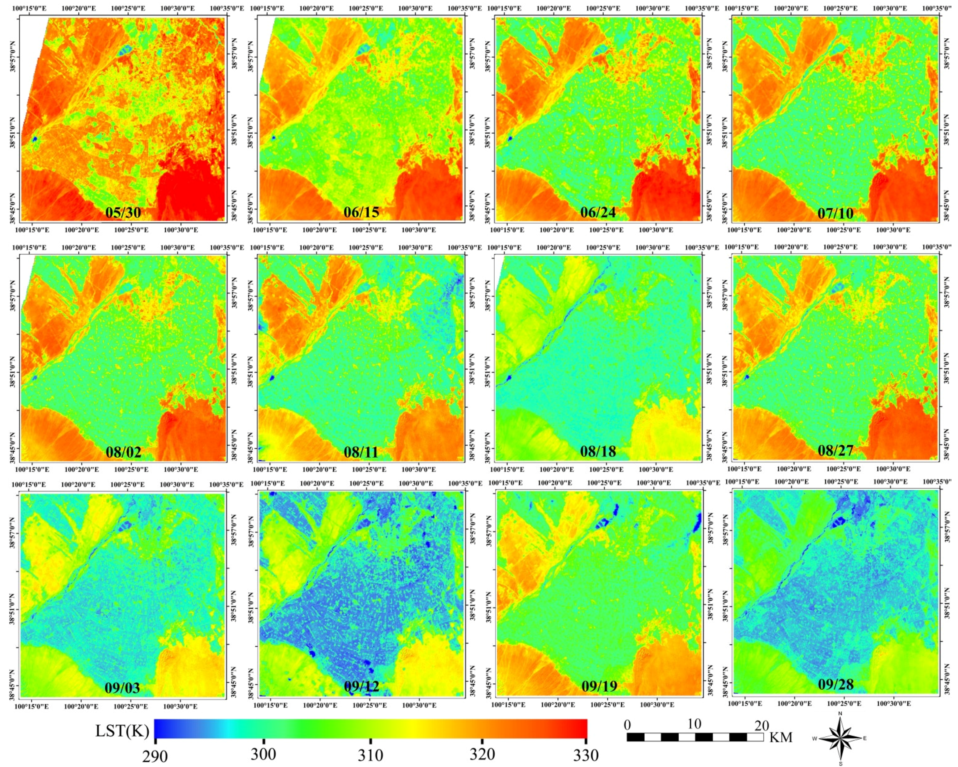
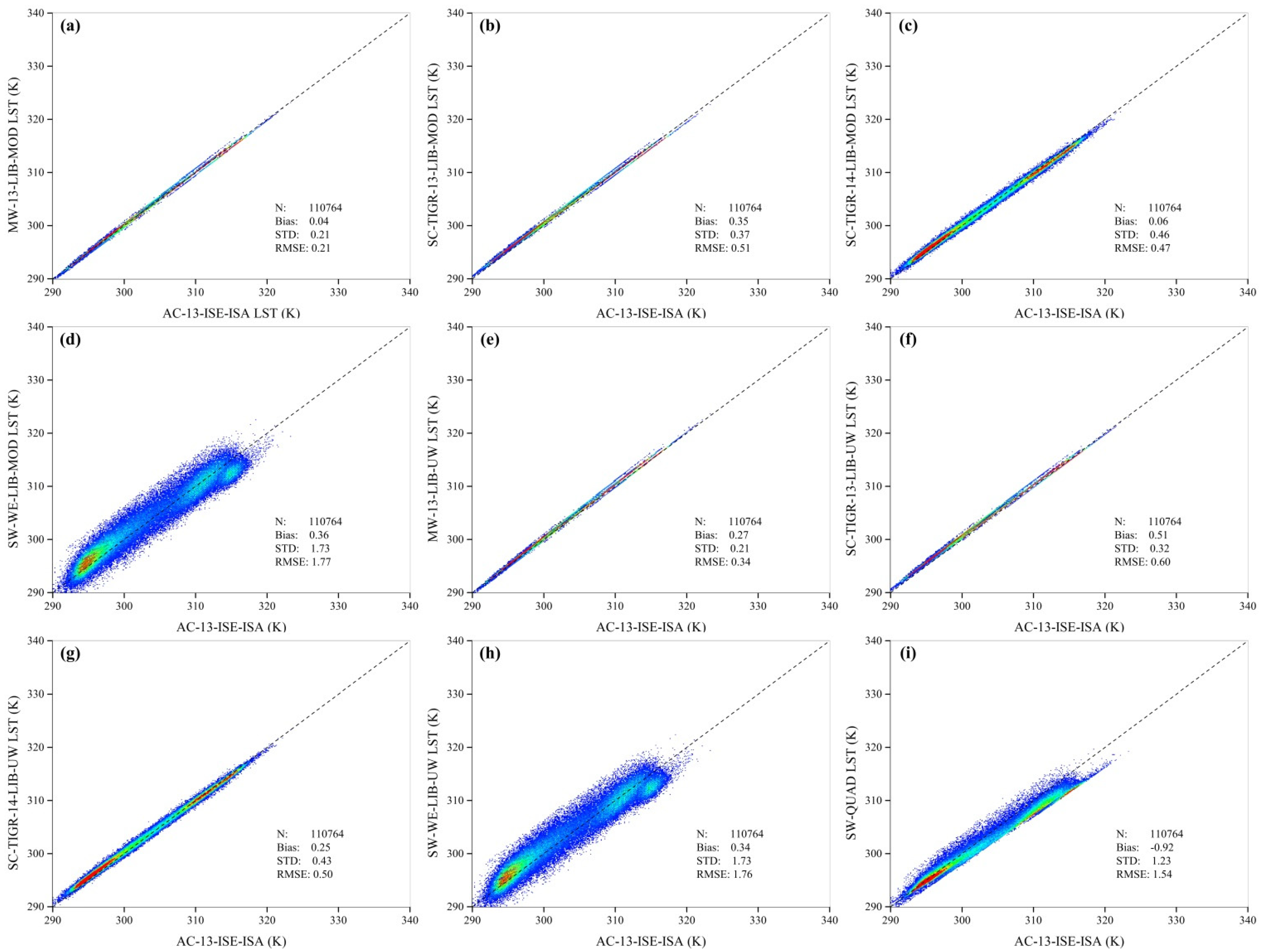
4.3. Comparisons between ASTER LST Images

The analysis in Section 4.2 reveals that many factors influence the validations of ASTER LSTs with in situ measured LSTs. Therefore, the radiance-based method is used simply here [40]. ASTER channel 13 is used as the reference band to calculate the ground LSTs because it suffers fewer atmospheric influences than the other channels. In addition, AC-13-ISE-ISA LST is selected as the reference LST because it has been found to be more accurate than most of the methods. LSTs from MW-13-LIB-MOD, SC-TIGR-13-LIB-MOD, SC-TIGR-14-LIB-MOD, SW-WE-LIB-MOD, MW-13-LIB-UW, SC-TIGR-13-LIB-UW, SC-TIGR-14-LIB-UW, SW-WE-LIB-UW, and SW-QUAD are selected for comparison, according to the evaluations based on the in situ LST measurements. Note that we do not select the methods with the in situ LSEs and atmospheric parameters here because these two datasets are commonly unavailable in actual applications. The three case studies selected are 30 May, 11 August, and 12 September because these three dates had different surface characteristics and meteorological conditions, as shown in Figure 6; the scatter plots for 30 May, 11 August, and 12 September are shown in Figure 7, Figure 8 and Figure 9, respectively.
Figure 7. Scatter plots between the LSTs estimated with AC-13-ISE-ISA and other methods on 30 May for the entire study area. STD here denotes the standard deviation of LST errors. (a) MW-13-LIB-MOD, (b) SC-TIGR-13-LIB-MOD, (c) SC-TIGR-14-LIB-MOD, (d) SW-WE-LIB-MOD, (e) MW-13-LIB-UW, (f) SC-TIGR-13-LIB-UW, (g) SC-TIGR-14-LIB-UW, (h) SW-WE-LIB-UW, (i) SW-QUAD.
Remotesensing 07 07126 g007
The scatter plots for the SW-WE method and the SW-QUAD method have larger standard deviations than the MW and SC methods. The term (Tbi − Tbj) in the expressions and the different atmospheric influences and noise in these two channels contribute to the high standard deviations. The SW-WE and SW-QUAD methods also have larger deviations than the AC-13-ISE-ISA LST. The RMSE values range from 2.96 K to 3.58 K on 30 May, from 3.37 K to 4.36 K on 11 August, and from 1.54 K to 1.77 K on 12 September. These large RMSE values demonstrate that the two SW methods are limited in their ability to remove the atmospheric influences, particularly in the middle stage of the maize growth. Therefore, these two SW methods should be treated with caution when used to estimate the evapotranspiration of agricultural fields in the study area.
Figure 8. Scatter plots between the LSTs estimated with AC-13-ISE-ISA and other methods on 11 August for the entire study area. STD here denotes the standard deviation of LST errors. (a) MW-13-LIB-MOD, (b) SC-TIGR-13-LIB-MOD, (c) SC-TIGR-14-LIB-MOD, (d) SW-WE-LIB-MOD, (e) MW-13-LIB-UW, (f) SC-TIGR-13-LIB-UW, (g) SC-TIGR-14-LIB-UW, (h) SW-WE-LIB-UW, (i) SW-QUAD.
Remotesensing 07 07126 g008
LSTs estimated based on the AC, MW, and SC methods are generally in good agreement because these methods are all applied to a single TIR channel. The MW and SC methods remove the atmospheric influences similarly to the AC method, according to their basic assumptions. Compared with channel 13, scatter plots for the LST calculated from channel 14 using the SC method have slightly dispersive patterns; see Figure 7c,g, Figure 8c,g, and Figure 9c,g. These dispersive patterns also result from the different spectral response features, atmospheric influences, and noise in channels 13 and 14. The MW method seems to yield lower LST estimations than AC-13-ISE-ISA when WVC is on high level, and vice versa. The biases of the MW method are −1.21 K and −0.37 K on May 30, −1.87 K and −2.07 K on 11 August, and 0.04 K and 0.27 K on 12 September. This phenomenon also occurs when comparing the in situ LST measurements (see Table 3 and Table 6). In contrast, the SC method generally has higher LST estimations than AC-13-ISA-ISE. Therefore, we assume that the MW method excessively corrects the atmospheric influences when the WVC is increasing, while the SC method insufficiently corrects the influences.
Figure 9. Scatter plots between the LSTs estimated with AC-13-ISE-ISA and other methods on 12 September for the entire study area. STD here denotes the standard deviation of LST errors. (a) MW-13-LIB-MOD, (b) SC-TIGR-13-LIB-MOD, (c) SC-TIGR-14-LIB-MOD, (d) SW-WE-LIB-MOD, (e) MW-13-LIB-UW, (f) SC-TIGR-13-LIB-UW, (g) SC-TIGR-14-LIB-UW, (h) SW-WE-LIB-UW, (i) SW-QUAD.
Remotesensing 07 07126 g009

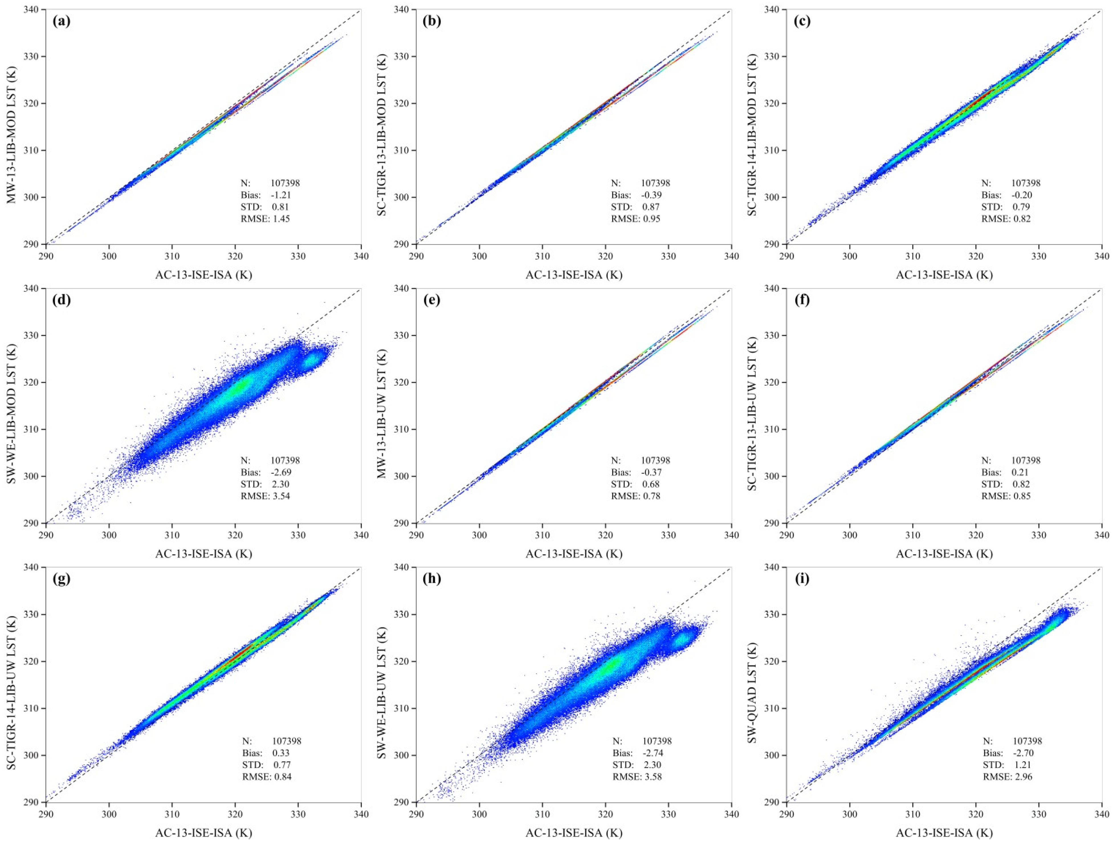
4.4. Evaluation with the Simulation Dataset

Based on the simulation dataset, the previous methods applied to different channels are compared. The bias and RMSE values are shown in Table 7. Note that the temperature-emissivity separation method is not considered here because its performance is strongly related to the preliminary atmospheric correction. In addition, our purpose is to evaluate the methods’ abilities to remove the atmospheric influences. Therefore, the other sources of atmospheric profiles, i.e., MOD and UW, are not considered.
The methods applied to a single channel are expected to have better accuracies in channel 13 than in channel 14 due to the weaker atmospheric influences in the former channel, as described in Section 4.2. The AC method has the highest accuracy, with no systematic error and an RMSE of 0.08 K. The error in the AC method may be caused by noise in the simulated brightness temperatures. The MW method underestimated the LSTs, with a bias of approximately 0.7 K and an RMSE of approximately 0.9 K in channel 13. The difference in the RMSEs between using the WVC and τ derived from the atmospheric profiles and using the estimated values is approximately 0.1 K, demonstrating that this method is practical for actual applications because the in situ measured WVC and τ are commonly unavailable.
Table 7. Biases and RMSEs of the LSTs estimated with different methods based on the simulation dataset.
MethodWith derived WVC and τ from the Atmospheric Profile (K)With Estimated WVC and τ (K)
BiasRMSEBias (K)RMSE
AC-130.00.08----
AC-140.00.10----
MW-13−0.770.84−0.730.95
MW-14−0.951.02−0.901.15
SC-STD-131.251.261.201.33
SC-STD-141.411.431.331.56
SC-TIGR-131.021.031.001.15
SC-TIGR-141.271.281.231.45
SW-WE−1.061.37−1.061.37
Based on the simulation dataset, the SC method is less accurate than the MW method. The SC method systematically overestimates the LST shown by the biases. Similar overestimations are also found in Section 4.2. Higher accuracy is obtained by using the coefficients trained with the TIGR atmospheric profile database than those trained with the STD atmospheric profile database. Therefore, the coefficients of the TIGR database are recommended when using the SC method in the actual applications in our study area. The SW-WS method systematically underestimates the LST, with an accuracy of 1.37 K. No difference in the RMSEs is found when using the WVCs derived from the atmospheric profiles and the estimated WVCs. The SW-QUAD method also underestimates the LST, with a bias of −1.45 K; this method has the lowest accuracy among the methods considered here, with an RMSE of 1.91 K. We believe that the low accuracy is attributable to the lack of LSE and atmospheric parameters considered. Higher accuracy may be obtained if a look-up table method is constructed for different land cover types and atmospheric conditions.
According to previous accuracy evaluations, the sensitivity analysis of the LSE uncertainty is conducted for the AC-13, MW-13, SC-TIGR-13, and SW-WE methods; the WVC uncertainty analysis is conducted for these methods, except for the AC-13 method, which requires an atmospheric profile as input. The results of the sensitivity analysis are shown in Figure 10. The SW-WE method is the most sensitive method to the LSE uncertainty. The AC, MW, and SC methods have similar sensitivities to the LSE uncertainty, and the LST uncertainty is approximately 1.0 K when the LSE uncertainty is approximately 0.02. This LSE accuracy can be obtained using the NDVITHM method [41]. Compared with the other three methods, the SC-TIGR-13 method is the least sensitive to the LSE uncertainty in wet atmospheric conditions. However, the SC method is sensitive to the WVC uncertainty for the two selected dates because its ability to remove the atmospheric influences depends on the atmospheric functions of the WVC. The MW method is moderately sensitive to the WVC uncertainty in dry atmospheric conditions. The SW-WE method is only slightly sensitive to the WVC uncertainty. Therefore, the conventional meteorological observations can be used to estimate the WVC required by the MW and SW-WE methods during the vegetation growth in the study area.
Figure 10. Sensitivities of the methods. (a) LST uncertainty induced by LSE uncertainty, (b) LST uncertainty induced by WVC uncertainty.
Remotesensing 07 07126 g010

5. Discussion

Validation and performance evaluations are beneficial for developing LST methods and improving existing LST products. Thermal observations from ASTER are a good source for monitoring the evapotranspiration in agricultural fields. Although many LST methods have been proposed for global applications, they perform differently in different areas. Our previous research on Landsat-5 TM data in the upper reach of HRB (with an elevation approximately 2600–3400 m) shows that the SC method has similar accuracy to that of the AC method and better accuracy than the MW method [9]. The study area in the current research has a warmer and wetter atmosphere than the upper reach of HRB, and we find that methods perform differently. Similar findings exist when comparing our research with that of Jiménez-Muñoz and Sobrino [14,15]. Therefore, a preliminary comparison between different LST methods is important if one requires high LST accuracy.
For validation and performance evaluation purposes, accuracy is an important evaluation indicator. Although there have been several methods proposed by scientists for validation purposes, e.g., the radiance-based method and scene-based method [7,40,42], the temperature-based method is required to provide a direct comparison between the remotely sensed LSTs and the in situ measurements. The temperature-based method faces many limitations, including surface heterogeneity, scale matches between the pixel and the ground site, and the viewing and illumination geometries [43]. As shown in Table 3, Table 4, Table 5 and Table 6, the influences of surface heterogeneity on the validation are significant in our study area. By removing the samples with large NDVI and LST heterogeneity, the potential influences of heterogeneity are reduced. The influence of scale mismatches is assumed to be small because the radiometers’ FOVs have scales comparable to those of the pixels. The influence from the viewing and illumination geometry for the sun-surface-ASTER sensor may be slight because the ASTER’s observation is approximately at the nadir point. However, uncertainty may result from the different view geometries between the ASTER and the longwave radiometer. The former provides a directional observation, while the latter provides a hemispherical observation. This issue cannot be accurately quantified at this stage due to lack of the directional emissivity at the ground sites. In addition, determinations of the LSEs in the FOVs and the accuracies of the longwave measurements also induce validation uncertainties [12].
Irrigation frequently occurred in the oasis agricultural fields of the study area. The spatial variations of the soil moisture induced by irrigation may aggravate the ground sites’ surface heterogeneity. In this research, the influences of irrigation on the ground sites’ surface heterogeneity were indirectly considered through examinations on the TASI LST and ASTER NDVI because both LST and NDVI are sensitive to soil background moisture [44]. When the maize fields are fully vegetated, the influences of soil moisture on surface heterogeneity decrease to a very low level due to canopy shielding.
In an actual application, the selection of the LST method depends on whether the method yields acceptable accuracies. For example, Timmermans et al. (2007) reported that a 3 K deviation in the LST can induce a 75% deviation in the sensible heat flux of a two-source model [45]. By selecting Beijing as the study area, Zhou et al. (2010) found that a 1%–2% error in the LST can induce 17.8–48.1 W/m2 and 11.6–32.3 W·m2 errors in the net radiation flux in summer and winter, respectively [46]. In fact, the method’s accuracy relies on its ability to remove atmospheric influence and emissivity, its sensitivity to errors in the parameters, and the accuracies of the input parameters. As for the methods examined in this research, the AC and MW methods have the highest accuracies in general, even when they are executed with alternative inputs. Although the SW-QUAD method is highly accurate when compared with the in situ LST measurements, it is the least accurate among the methods when compared with the simulation dataset. We infer that its high accuracy may result from counteraction of the uncertainties of the algorithm and the in situ measured LSTs.
In addition to the accuracy, we suggest that two other indicators should be considered in evaluating the methods’ performances. The first indicator is sensitivity. A good method should generate stable LSTs when the input parameters have acceptable errors. Therefore, we suggest that a method’s sensitivity is its robustness. For the methods examined in this research, two important input parameters are the LSE and atmospheric profile/parameter. The SW-WE method significantly relies on the LSE uncertainty. The MW, SC, and AC methods have relatively lower sensitivities to the LSE uncertainty. In cases without in situ measured LSEs, the LSEs calculated from the NDVI threshold method may be a good choice. As for the WVC uncertainty, the MW and SW-WE methods are not very sensitive. Thus, the MW method is relatively insensitive to the uncertainties in the input parameters.
The second indicator is the method’s practicability or simplicity for a specific thermal sensor. The ASTER standard LST products need to be purchased from the ASTER Ground Data System. Therefore, if a method can be used by common users to calculate the LSTs, such a method should be practical and simple, and the input parameters can be easily obtained. All the methods examined in this research have this advantage, except for the AC method, which requires that the user be familiar with an atmospheric transfer model, such as MODTRAN.
The calculated ASTER LSTs are well able to estimate the field-scale evapotranspiration in the study area, with finer spatial resolutions than most of the current operational LST products, e.g., the MODIS LST product. In addition to the spatial resolution, another evapotranspiration consideration is its temporal resolution, depending on the LSTs with the same temporal resolutions. For the diurnal change in evapotranspiration, a diurnal temperature cycle model is helpful. This type of model can be applied to the LSTs acquired by a satellite sensor with multiple observations in the same area in a diurnal cycle, such as the thermal sensors on board the geostationary satellites [47]. However, the current diurnal cycle models have limited abilities in parameterizing the influences of varying meteorological conditions, e.g., wind and clouds. In addition, such LST products have low spatial resolutions, which cannot provide enough spatial details at the field scale. Constructing LSTs with high spatial and temporal resolutions and acceptable accuracies for agricultural areas remains a topic of ongoing research.

6. Conclusions

By selecting a flat agricultural oasis and the surrounding bare land as the study area, this study evaluated the performance of four methods that can be applied to ASTER data to estimate the LST: the atmospheric correction (AC) method, the mono-window (MW) method, the single-channel (SC) method, and the split-window (SW) method. The first three methods depend on a single TIR channel of ASTER, while the last method depends on two adjacent channels. Evaluations are conducted based on in situ LST measurements from 19 AMSs and a simulation dataset generated from MODTRAN5.2.2 code. The ASTER standard LST products are also evaluated with in situ LST measurements.
Evaluations of these methods were conducted for different combinations of channels and input parameters. The results demonstrated that the SW-QUAD method has the best accuracy, with a bias and RMSE of 0.49 K and 1.38 K, respectively, when compared with the in situ measured LSTs at the oasis sites. However, this method should be used with caution because we find it has poor accuracy when compared with the simulation dataset. As with the SW-QUAD method, the SW-WE method has the advantage of simplicity. When compared with measurements from the oasis sites, its RMSE is about 1.68 K when in situ measured LSEs are available. However, its accuracy decreases significantly if emissivities from spectral libraries are used. One possible reason for this decrease may be the shortcomings of the corresponding emissivities in the spectral libraries. Another possible reason may be the uncertainties of the estimated fractional vegetation abundance. For the ASTER standard LST product, the bias and RMSE are 1.39 K and 2.20 K, respectively.
For the AC, MW, and SC methods, the results demonstrated that the LSTs estimated from channel 13 are more accurate than those from channel 14 in general cases because channel 14 experiences stronger atmospheric influences. When the in situ measured atmospheric profiles are available, the AC method has the highest accuracy, with an RMSE of about 1.4–1.5 K at the homogenous oasis sites. For actual applications without such measurements, its practicability is low. The MW method is highly accurate when using alternative LSEs and estimated atmospheric parameters as inputs; the RMSE is around 1.5–1.6 K. An evaluation based on the simulation confirmed its solid performance in estimating the LST for the study area. The advantage of the SC method is its simplicity because it relies on a single atmospheric parameter (i.e., WVC). But it shows a significant overestimation of LSTs. Therefore, the AC and MW methods are recommended to users who are interested in modeling eco-hydrological processes in the middle reach of the HRB. Selecting methods depends on the availabilities of in situ measured atmospheric profiles and LSEs. With these methods, evapotranspiration maps with a 90-m resolution can be obtained, which is higher than those of most of the current satellite thermal images.

Acknowledgements

We thank all the scientists, engineers, and students who participated in HiWATER field campaigns. This work was supported by the National Natural Science Foundation of China (91125002 and 41371341), the Chinese State Key Basic Research Project (2013CB733406), and the Opening Funding of State Key Laboratory for Remote Sensing Science (OFSLRSS201313). The MOD07_L2 products were provided by NASA’s Earth Observing System Data and Information System. The component spectrum dataset was provided by the MODIS UCSB Emissivity Library. The UW atmospheric profiles were provided by the Department of Atmospheric Science, University of Wyoming. The ASTER images were purchased from the ASTER Ground Data System. We thank the anonymous referees for their constructive criticism and comments.

Author Contributions

Ji Zhou wrote the manuscript and was responsible for research design and analysis. Mingsong Li was responsible for implementation of different methods, data preparation, and processing. Shaomin Liu contributed to research design, provided the in situ measurements of land surface temperatures (LSTs), and gave constructive comments and suggestions. Zhenzhen Jia processed the in situ LSTs and some of the land surface emissivities. Yanfei Ma contributed by processing the remote sensing data.

Acronyms

AC
atmospheric correction
AMS
Automatic Meteorological Station
HiWATER
Heihe Watershed Allied Telemetry Experimental Research
HRB
Heihe River basin
ISA
in situ measured atmospheric profile
ISE
in situ measured land surface emissivity
LIB
land surface emissivity determined based on the MODIS UCSB Emissivity Library
LSE
land surface emissivity
LST
land surface temperature
MOD
MOD07_L2 product
MUSOEXE
Multi-Scale Observation Experiment on Evapotranspiration
MW
mono-window
NDVI
normalized difference vegetation index
SC
single-channel
STD
standard atmospheric profiles in MODTRAN code
SW
split-window
SW-QUAD
split-window method without the water vapor content and land surface emissivity as the inputs
SW-WE
split-window method with the water vapor content and land surface emissivity as the inputs
TIGR
Thermodynamic Initial Guess Retrieval (TIGR)
TIR
thermal infrared
UW
University of Wyoming
WVC
water vapor content

Conflicts of Interest

The authors declare no conflict of interest.

References

  1. Ma, Y.; Liu, S.; Zhang, F.; Zhou, J.; Jia, Z.; Song, L. Estimations of regional surface energy fluxes over heterogeneous oasis–desert surfaces in the middle reaches of the Heihe River during HiWATER-MUSOEXE. IEEE Geosci. Remote Sens. Lett. 2015, 12, 671–675. [Google Scholar] [CrossRef]
  2. Berk, A.; Bernstein, L.S.; Anderson, G.P.; Acharya, P.K.; Robertson, D.C. MODTRAN cloud and multiple scattering upgrades wit application to AVIRIS. Remote Sens. Environ. 1998, 65, 367–375. [Google Scholar]
  3. Li, Z.L.; Tang, B.H.; Wu, H.; Ren, H.; Yan, G.; Wan, Z.; Trigo, I.F.; Sobrino, J.A. Satellite-derived land surface temperature: Current status and perspectives. Remote Sens. Environ. 2013, 131, 14–37. [Google Scholar] [CrossRef]
  4. Sobrino, J.A.; Kharraz, J.E.L. Surface temperature and water vapour retrieval from MODIS data. Int. J. Remote Sens 2003, 24, 5161–5182. [Google Scholar]
  5. Yu, Y.; Privette, J.L.; Pinheiro, A.C. Evaluation of split-window land surface temperature algorithms for generating climate data records. IEEE Trans. Geosci. Remote Sens. 2008, 46, 179–192. [Google Scholar] [CrossRef]
  6. Yu, Y.; Tarpley, D.; Privette, J.; Goldberg, M.D.; Varma Raja, M.K.R.; Vinnikov, K.Y.; Xu, H. Developing algorithm for operational GOES-R land surface temperature product. IEEE Trans. Geosci. Remote Sens. 2009, 47, 936–951. [Google Scholar]
  7. Guillevic, P.C.; Biard, J.C.; Hulley, G.C.; Privette, J.L.; Hook, S.J.; Olioso, A.; Göttsche, F.M.; Radocinski, R.; Román, M.O.; Yu, Y.; et al. Validation of land surface temperature products derived from the Visible Infrared Imaging Radiometer Suite (VIIRS) using ground-based and heritage satellite measurements. Remote Sens. Environ. 2014, 154, 19–37. [Google Scholar] [CrossRef]
  8. Sobrino, J.A.; Jiménez-Muñoz, J.C.; Paolini, L. Land surface temperature retrieval from Landsat TM 5. Remote Sens. Environ. 2004, 90, 434–440. [Google Scholar] [CrossRef]
  9. Zhou, J.; Li, J.; Zhang, L.; Hu, D.; Zhan, W. Intercomparison of methods for estimating land surface temperature from a Landsat-5 TM image in an arid region with low water vapour in the atmosphere. Int. J. Remote Sens. 2012, 33, 2582–2602. [Google Scholar] [CrossRef]
  10. Yamaguchi, Y.; Anne, B.; Kahle, H.T. Overview of Advanced Spaceborne Thermal Emission and Reflection Radiometer (ASTER). IEEE Trans. Geosci. Remote Sens. 1998, 36, 1062–1071. [Google Scholar] [CrossRef]
  11. Gillespie, A.; Rokugawa, S.; Matsunaga, T.; Cothern, J.S.; Hook, S.; Kahle, A.B. A temperature and emissivity separation algorithm for Advanced Spaceborne Thermal Emission and Reflection Radiometer (ASTER) images. IEEE Trans. Geosci. Rem. Sens. 1998, 36, 1113–1126. [Google Scholar] [CrossRef]
  12. Wang, K.; Liang, S. Evaluation of ASTER and MODIS land surface temperature and emissivity products using long-term surface longwave radiation observations at SURFRAD sites. Remote Sens. Environ. 2009, 113, 1556–1565. [Google Scholar] [CrossRef]
  13. Pu, R.; Gong, P.; Michishita, R.; Sasagawa, T. Assessment of multi-resolution and multi-sensor data for urban surface temperature retrieval. Remote Sens. Environ. 2006, 104, 211–225. [Google Scholar] [CrossRef]
  14. Jiménez-Muñoz, J.C. , Sobrino, J.A. Feasibility of retrieving land-surface temperature from ASTER TIR bands using two-channel algorithms: A case study of agricultural areas. IEEE Geosci. Remote Sens. 2007, 4, 60–64. [Google Scholar] [CrossRef]
  15. Jiménez-Muñoz, J.C.; Sobrino, J.A. A single-channel algorithm for land-surface temperature retrieval from ASTER data. IEEE Geosci. Remote Sens. 2010, 4, 60–64. [Google Scholar] [CrossRef]
  16. Li, X.; Cheng, G.; Liu, S.; Xiao, Q.; Ma, M.; Jin, R.; Che, T.; Liu, Q.; Wang, W.; Qi, Y.; et al. Heihe watershed allied telemetry experimental research (HiWATER): Scientific objectives and experimental design. Bull. Am. Meteorol. Soc. 2013, 94, 1145–1160. [Google Scholar] [CrossRef]
  17. Xu, Z.; Liu, S.; Li, X.; Shi, S.; Wang, J.; Zhu, Z.; Xu, T.; Wang, W.; Ma, M. Intercomparison of surface energy flux measurement systems used during the HiWATER-MUSOEXE. J. Geophys. Res. 2013, 118, 13140–13157. [Google Scholar] [CrossRef]
  18. Liu, S.; Xu, Z.; Wang, W.; Bai, J.; Jia, Z.; Zhu, M.; Wang, J. A comparison of eddy-covariance and large aperture scintillometer measurements with respect to the energy balance closure problem. Hydrol. Earth Syst. Sc. 2011, 15, 1291–1306. [Google Scholar] [CrossRef]
  19. Yan, K.; Ren, H.; Hu, R.; Mu, X.; Liu, Z.; Yan, G. Error analysis for emissivity measurement using FTIR spectrometer. In Proceedings of IEEE International Geoscience and Remote Sensing Symposium, Melbourne, VIC, Australia, 21–26 July 2013; pp. 3080–3083.
  20. Mu, X.; Hu, R.; Huang, S.; Chen, Y. HiWATER: Dataset of Emissivity in the Middle Reaches of the Heihe River Basin in 2012; Cold and Arid Regions Science Data Center at Lanzhou: Lanzhou, China, 2012. [Google Scholar]
  21. Berry, T.E.; Melton, R.E. Multi-spectral thermal image analysis of natural backgrounds and targets. Proc. SPIE 2005, 5794, 866–874. [Google Scholar]
  22. Mu, X.; Huang, S.; Chen, Y. HiWATER: Dataset of Fractional Vegetation Cover in the Middle Reaches of the Heihe River Basin; Cold and Arid Regions Science Data Center at Lanzhou: Lanzhou, China, 2012. [Google Scholar]
  23. Liu, Y.; Mu, X.; Wang, H.; Yan, G. A novel method for extracting green fractional vegetation cover from digital images. J. Veg. Sci. 2012, 23, 406–418. [Google Scholar] [CrossRef]
  24. Zhou, J.; Zhang, X.; Zhan, W.; Zhang, H. Land surface temperature retrieval from MODIS data by integrating regression models and the genetic algorithm in an arid region. Remote Sens. 2014, 6, 5344–5367. [Google Scholar] [CrossRef]
  25. Xiao, Q.; Wen, J. HiWATER: Land Surface Temperature Product in the Middle Reaches of the Heihe River Basin (30th, June, 2012); Cold and Arid Regions Science Data Center at Lanzhou: Lanzhou, China, 2012. [Google Scholar]
  26. Xiao, Q.; Wen, J. HiWATER: Land Surface Temperature Product in the Middle Reaches of the Heihe River Basin (10th, July, 2012); Cold and Arid Regions Science Data Center at Lanzhou: Lanzhou, China, 2012. [Google Scholar]
  27. Wang, H.; Xiao, Q.; Li, H.; Zhong, B. Temperature and emissivity separation algorithm for TASI airborne thermal hyperspectral data. In Proceedings of IEEE International Geoscience and Remote Sensing Symposium, Vancouver, BC, Canada, 24–29 July 2011; pp. 1075–1078.
  28. TASI-600 Thermal Airborne Broadband Imager. Available online: http://www.itres.com/tasi-600/ (accessed on 19 April 2015).
  29. Tan, J.; Ma, M. HiWATER: Dataset of Radiosonde Sounding Observations in Zhangye National Climate Observatory; Cold and Arid Regions Science Data Center at Lanzhou: Lanzhou, China, 2012. [Google Scholar]
  30. Ottlé, C.; Stoll, M. Effect of atmospheric absorption and surface emissivity on the determination of land surface temperature from infrared satellite data. Int. J. Rem. Sens. 1993, 14, 2025–2037. [Google Scholar] [CrossRef]
  31. Qin, Z.; Karnieli, A.; Berliner, P. A mono-window algorithm for retrieving land surface temperature from Landsat TM data and its application to the Israel-Egypt border region. Int. J. Remote Sens. 2001, 22, 3719–3746. [Google Scholar] [CrossRef]
  32. Jiménez-Muñoz, J.C.; Sobrino, J.A. A generalized single-channel method for retrieving land surface temperature from remote sensing data. J. Geophys. Res. 2003. [Google Scholar] [CrossRef]
  33. Chédin, A.; Scott, N.A.; Wahiche, C.; Moulinier, P. The improved initialization inversion method: A high resolution physical method for temperature retrievals from satellites of the Tiros-N series. J. Appl. Meteorol. 1985, 24, 128–143. [Google Scholar] [CrossRef]
  34. Chevallier, F.; Cheruy, F.; Scott, N.A.; Chédin, A. A neural network approach for a fast and accurate computation of a longwave radiative budget. J. Appl. Meteorol. 1998, 37, 1385–1397. [Google Scholar] [CrossRef]
  35. Jiménez-Muñoz, J.C.; Cristóbal, J.; Sobrino, J.A.; Sòria, G.; Ninyerola, M.; Pons, X. Revision of the single-channel algorithm for land surface temperature retrieval from Landsat thermal-infrared data. IEEE Trans. Geosci. Remote Sens. 2009, 47, 339–349. [Google Scholar] [CrossRef]
  36. Li, Z.L.; Wu, H.; Wang, N.; Qiu, S.; Sobrino, J.A.; Wan, Z.; Tang, B.H.; Yan, G. Land surface emissivity retrieval from satellite data. Int. J. Remote Sens. 2013, 34, 3084–3127. [Google Scholar] [CrossRef]
  37. Sobrino, J.A.; Raissouni, N. Toward remote sensing methods for land cover dynamic monitoring: Application to Morocco. Int. J. Remote Sens. 2000, 21, 353–366. [Google Scholar] [CrossRef]
  38. Yamaguchi, Y.; Fujisada, H.; Kahle, A.B.; Tsu, H.; Kato, M.; Watanabe, H.; Kudoh, S.M. ASTER instrument performance, operation status, and application to Earth sciences. In Proceedings of IEEE International Geoscience and Remote Sensing Symposium, Sydney, NSW, Australia, 9–13 July 2001; pp. 1215–1216.
  39. ASTER Product Guide. Available online: http://gds.aster.ersdac.jspacesystems.or.jp/ (accessed on 19 April 2015).
  40. Wan, Z.; Li, Z.L. Radiance-based validation of the V5 MODIS land-surface temperature product. Int. J. Rem. Sens. 2008, 29, 5373–5395. [Google Scholar] [CrossRef]
  41. Sobrino, J.A.; Raissouni, N.; Li, Z. A comparative study of land surface emissivity retrieval from NOAA data. Remote Sens. Environ. 2001, 75, 256–266. [Google Scholar] [CrossRef]
  42. Coll, C.; Wan, Z.; Galve, J.M. Temperature-based and radiance-based validation of the V5 MODIS land surface temperature product. J. Geophys. Res. 2009, 114. [Google Scholar] [CrossRef]
  43. Ermida, S.L.; Trigo, I.F.; DaCamara, C.S.; Göttsche, F.M.; Olesen, F.S.; Hulley, G. Validation of remotely sensed surface temperature over an oak woodland landscape—The problem of viewing and illumination geometries. Remote Sens. Environ. 2014, 148, 16–27. [Google Scholar] [CrossRef]
  44. Todd, S.W.; Hoffer, R.M. Responses of spectral indices to variations in vegetation cover and soil background. Photogramm. Eng. Remote Sens. 1998, 64, 915–921. [Google Scholar]
  45. Timmermans, W.J.; Kustas, W.P.; Anderson, M.C.; French, A.N. An intercomparison of the Surface Energy Balance Algorithm for Land (SEBAL) and Two-Source Energy Balance (TSEB) modeling schemes. Remote Sens. Environ. 2007, 108, 369–384. [Google Scholar] [CrossRef]
  46. Zhou, J.; Hu, D.; Weng, Q. Analysis of surface radiation budget during the summer and winter in the metropolitan area of Beijing, China. J. Appl. Remote Sens. 2010. [Google Scholar] [CrossRef]
  47. Zhou, J.; Chen, Y.; Zhang, X.; Zhan, W. Modelling the diurnal variations of urban heat islands with multi-source satellite data. Int. J. Remote Sens. 2013, 34, 7568–7588. [Google Scholar] [CrossRef]

