
On the Synergy of Airborne GNSS-R and Landsat 8 for Soil Moisture Estimation

 , ,
, ,  , and
, and
Abstract
:
1. Introduction
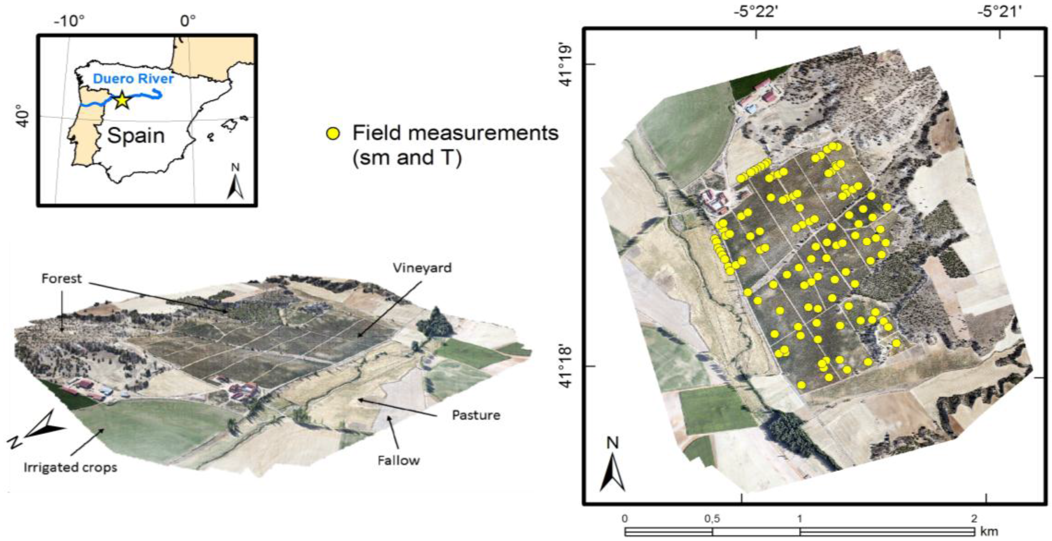
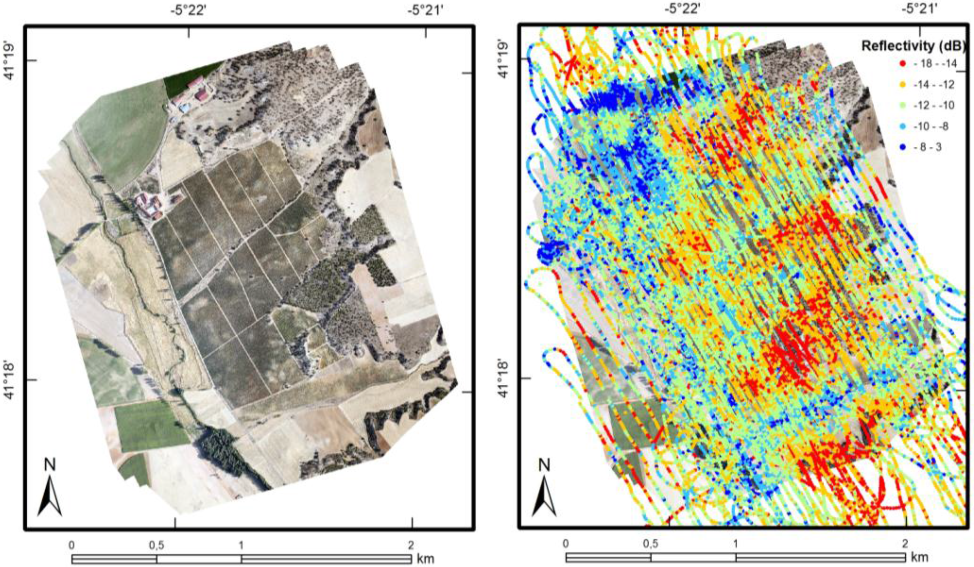
2. Airborne GNSS-R Observations and Field Campaign

3. Data and Methods
3.1. LARGO Pre-Processing


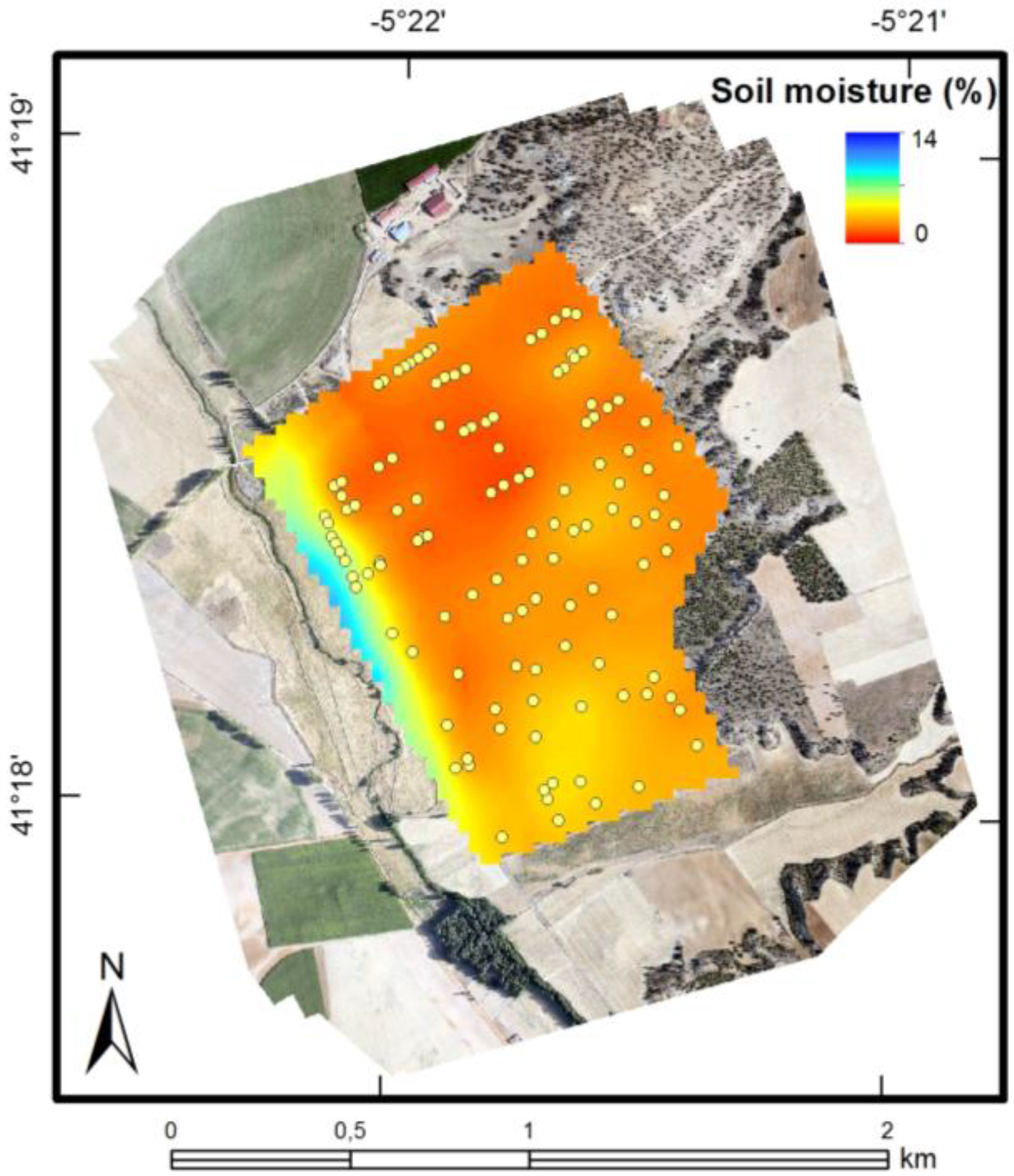
3.2. In situ Measurements Mapping

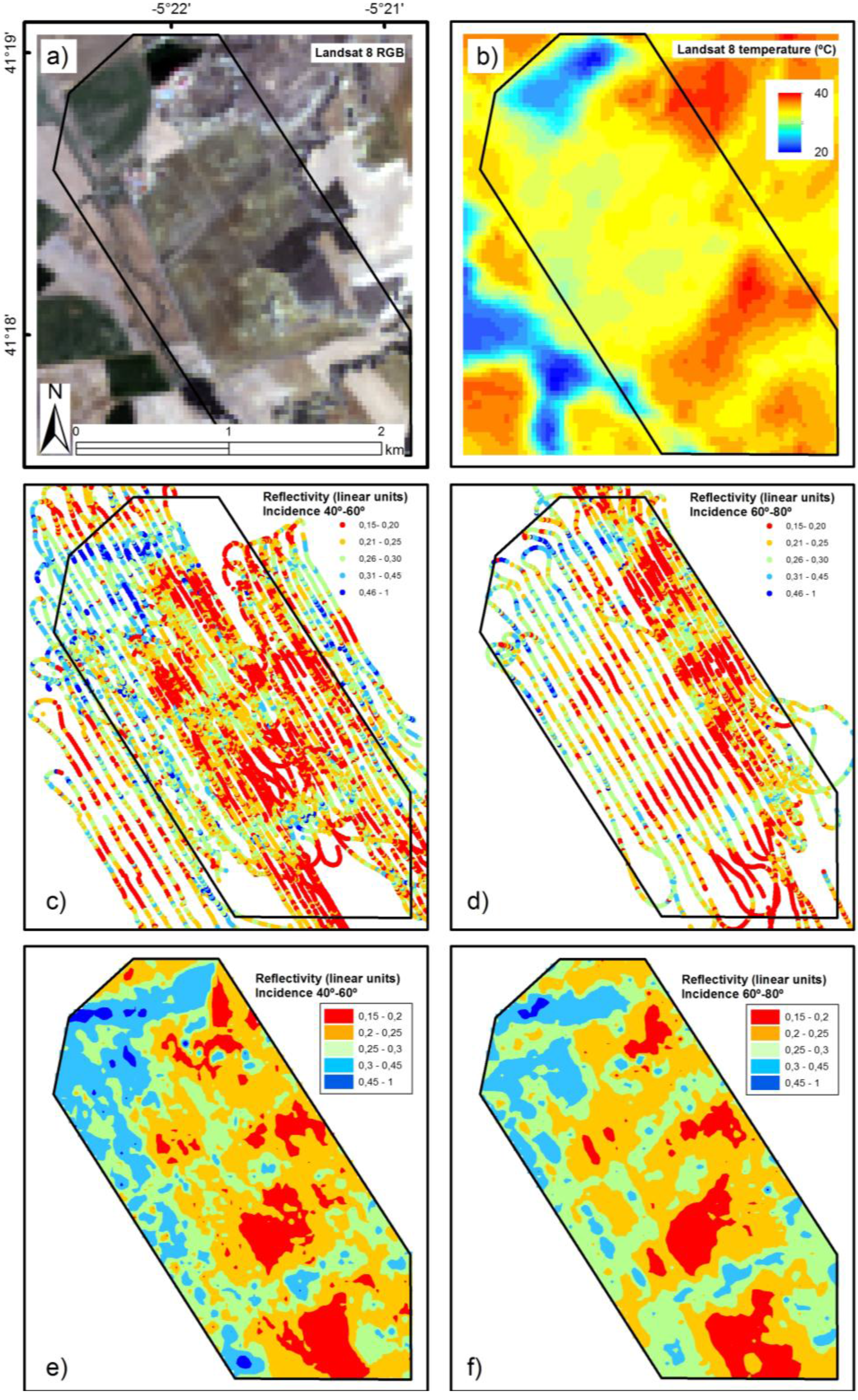
3.3. LANDSAT 8 Processing and Indices Retrieval
3.4. Statistical Analysis
3.4.1. Correlations
3.4.2. Linking Model
4. Results and Discussion
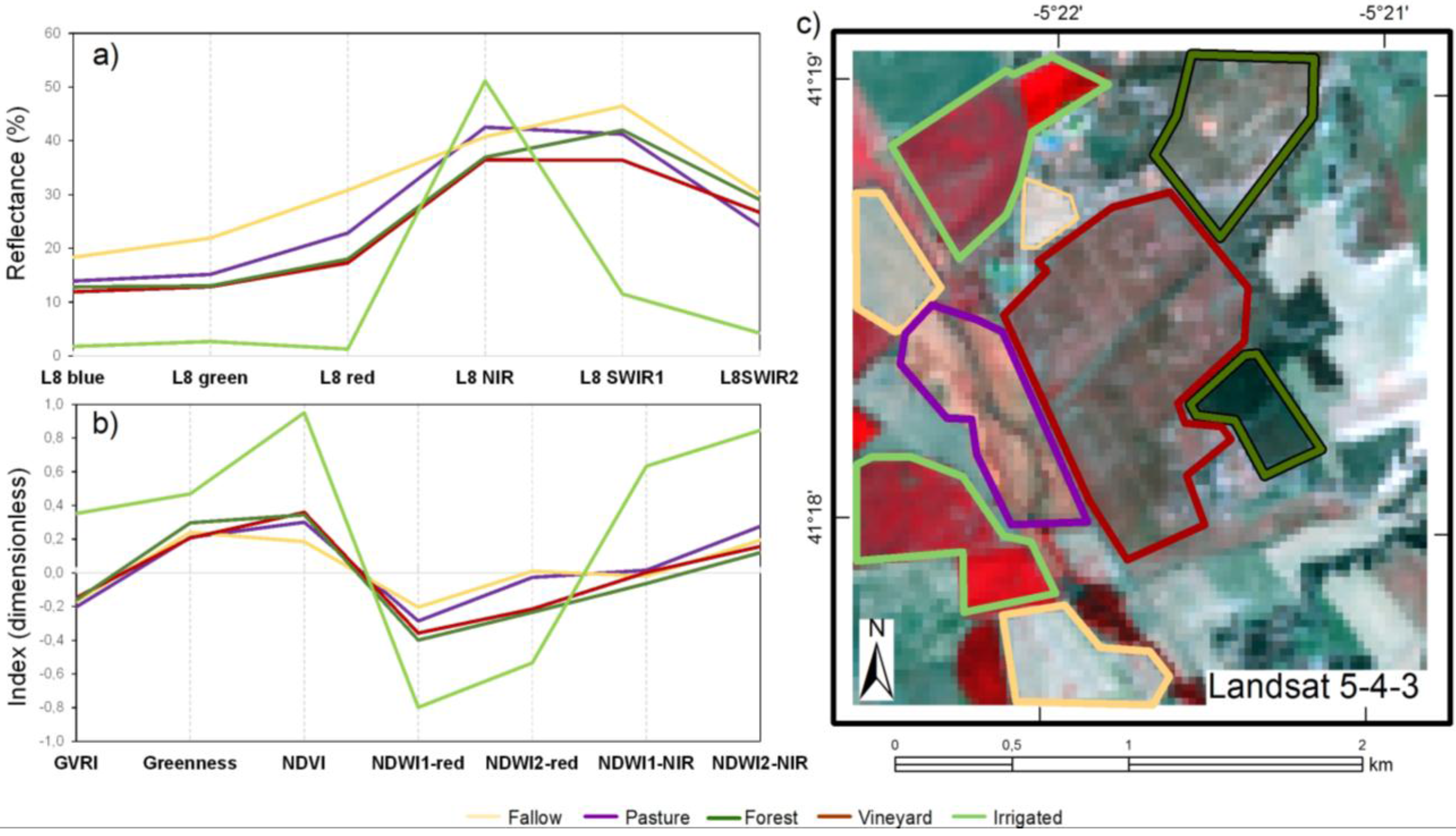
4.1. Landsat Reflectance and Indices for the Main Land Covers

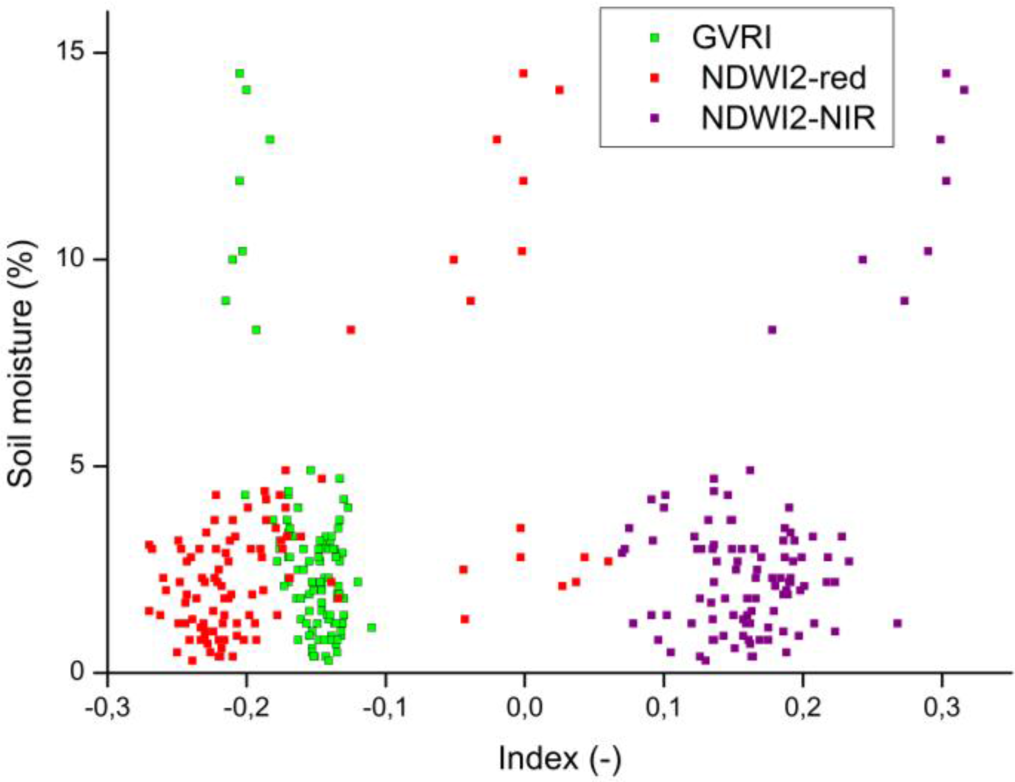
4.2. Correlation between Datasets

| R | Image (30 m) | In Situ (n = 119) | ||
|---|---|---|---|---|
| Soil Moisture | LST (L8) | Soil Moisture | T | |
| GVRI | −0.41 | 0.06 | −0.69 | 0.07 * |
| Greenness | −0.05 * | 0.14 | 0.07 * | 0.29 |
| NDVI | 0.01 * | −0.24 | −0.26 | −0.27 |
| NDWI1-red | 0.20 | −0.09 | 0.37 | 0.02 * |
| NDWI2-red | 0.58 | −0.17 | 0.59 | −0.06 * |
| NDWI1-NIR | 0.25 | −0.49 | 0.06 | −0.56 |
| NDWI2-NIR | 0.55 | −0.41 | 0.57 | −0.48 |
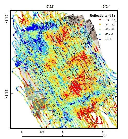
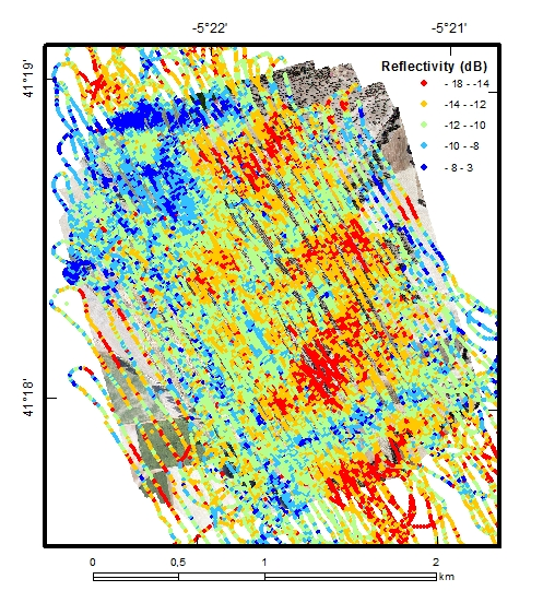
| LARGO 40-60 | 0.34 | −0.22 | 0.37 | −0.28 |
| LARGO 60-80 | 0.25 | −0.20 | 0.13 | −0.05 * |

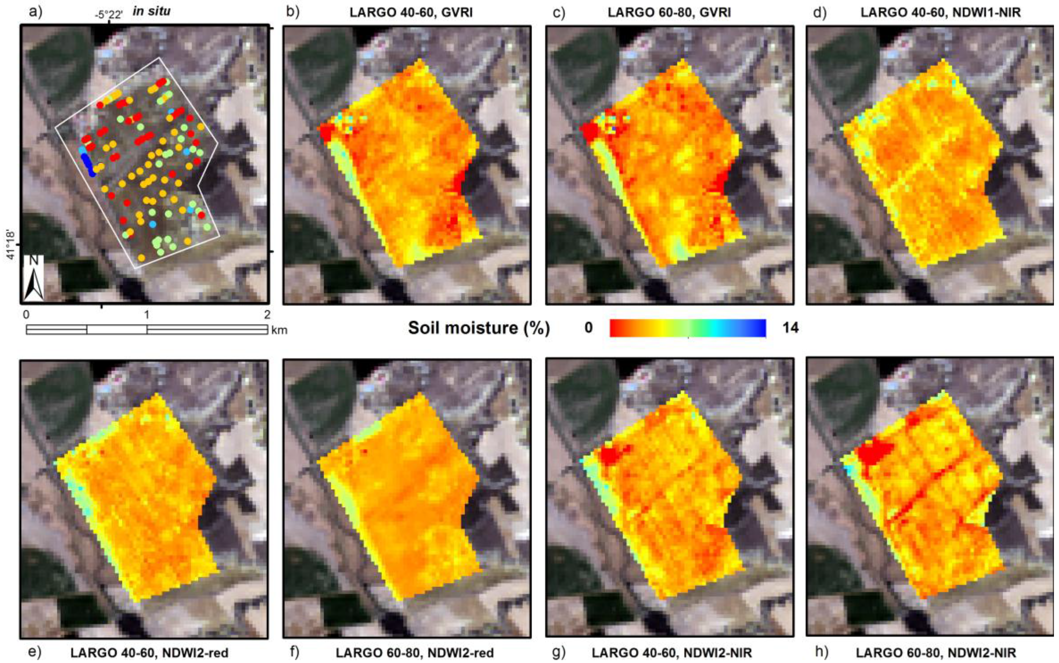
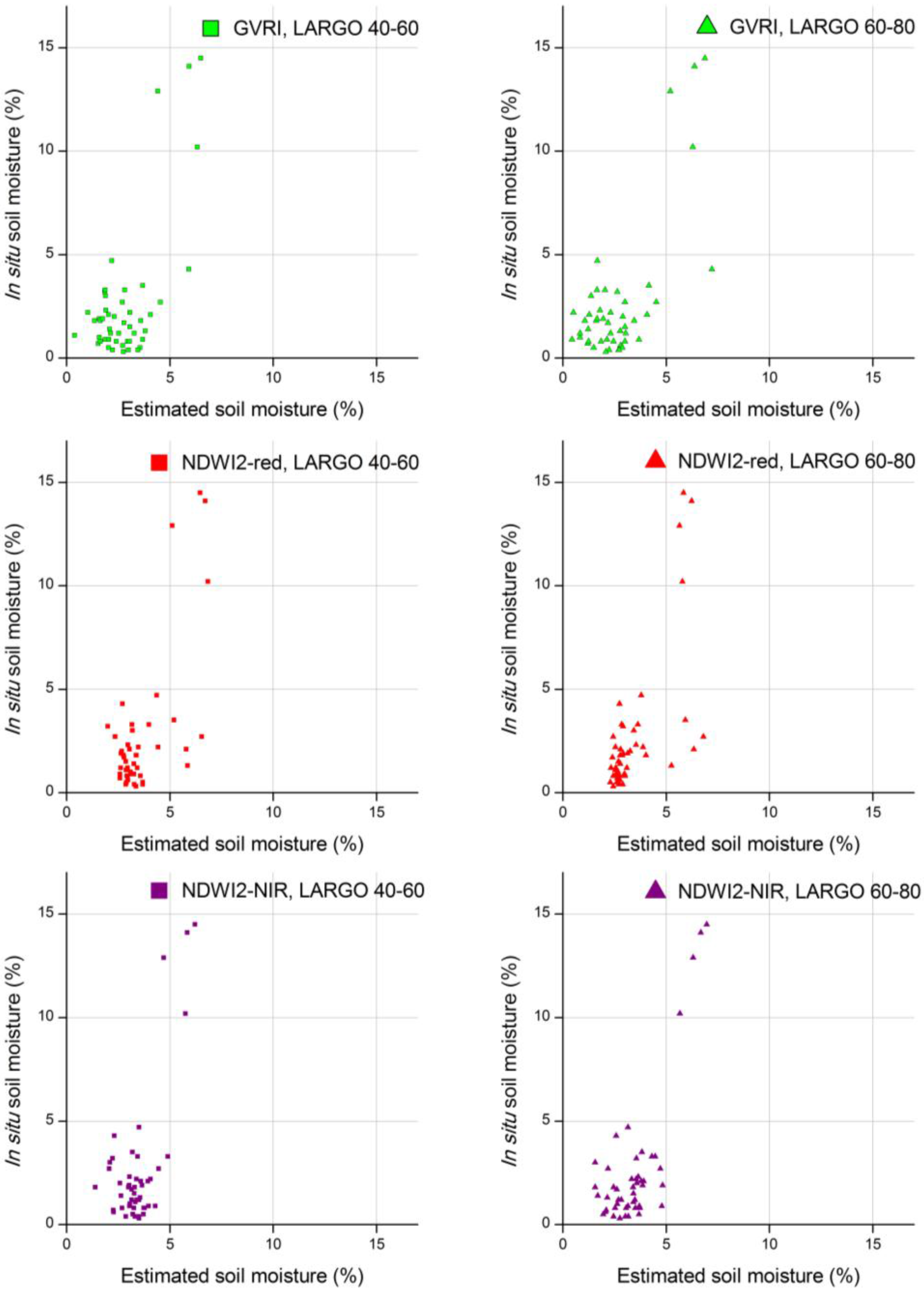
4.3. Linking Model Calculation and Validation
| Model Training In Situ Soil Moisture (n = 60) | LARGO 40-60 | LARGO 60-80 | ||||
|---|---|---|---|---|---|---|
| R | R2 | RMSE (%) | R | R2 | RMSE (%) | |
| GVRI | 0.69 | 0.48 | 1.60 | 0.69 | 0.48 | 1.60 |
| NDWI2-red | 0.64 | 0.42 | 1.69 | 0.52 | 0.27 | 1.89 |
| NDWI1-NIR | 0.51 | 0.27 | 1.90 | 0.12 * | 0.01 | 2.20 |
| NDWI2-NIR | 0.59 | 0.34 | 1.79 | 0.55 | 0.30 | 1.85 |
| R with the Training Sample (n = 60) | |||
|---|---|---|---|
| Model Options | Only Index | Index+LST | Index+LST+ LARGO 40-60 (LARGO 60-80) |
| GVRI | −0.66 | 0.67 | 0.69 (0.69) |
| NDWI2-red | 0.52 | 0.52 | 0.64 (0.52) |
| NDWI1-NIR | −0.10 * | 0.10 * | 0.51 (0.11 *) |
| NDWI2-NIR | 0.43 | 0.52 | 0.59 (0.55) |

| Model Validation In Situ Soil Moisture (Point Scale) | LARGO 40-60 | LARGO 60-80 | ||||
|---|---|---|---|---|---|---|
| R | bias (%) | RMSD (%) | R | bias (%) | RMSD (%) | |
| GVRI | 0.67 | −0.205 | 2.619 | 0.70 | 0.010 | 2.462 |
| NDWI2-red | 0.67 | −0.748 | 2.675 | 0.67 | −0.753 | 2.650 |
| NDWI1-NIR | 0.16 * | −0.353 | 3.284 | --- | --- | --- |
| NDWI2-NIR | 0.66 | −0.801 | 2.894 | 0.68 | −0.771 | 2.733 |

| Model Validation In situ Soil Moisture (Map) | LARGO 40-60 | LARGO 60-80 | ||||
|---|---|---|---|---|---|---|
| R | bias (%) | RMSD (%) | R | bias (%) | RMSD (%) | |
| GVRI | 0.37 | −0.046 | 1.632 | 0.28 | 0.107 | 1.844 |
| NDWI2-red | 0.57 | −0.571 | 1.394 | 0.57 | −0.315 | 1.267 |
| NDWI1-NIR | 0.23 * | −0.475 | 1.696 | --- | --- | --- |
| NDWI2-NIR | 0.45 | −0.287 | 1.520 | 0.35 | −0.150 | 1.839 |
5. Conclusions
Acknowledgments
Author Contributions
Conflicts of Interest
References
- Rodriguez-Alvarez, N.; Vall-llossera, M.; Camps, A.; Bosch-Lluis, X.; Monerris, A.; Ramos-Perez, I.; Valencia, E.; Marchan-Hernandez, J.F.; Martinez-Fernandez, J.; Baroncini-Turricchia, G.; et al. Land geophysical parameters retrieval using the interference pattern GNSS-R technique. IEEE Trans. Geosci. Remote Sens. 2011, 49, 71–84. [Google Scholar] [CrossRef]
- Kavak, A.; Vogel, W.J.; Xu, G. Using GPS to measure ground complex permittivity. Electron. Lett. 1998, 34, 254–255. [Google Scholar] [CrossRef]
- Larson, K.M.; Braun, J.J.; Small, E.E.; Zavorotny, V.U.; Gutmann, E.D.; Bilich, A.L. GPS multipath and its relation to near-surface soil moisture content. IEEE J. Sel. Top. Appl. Earth Obs. Remote Sens. 2010, 3, 91–99. [Google Scholar] [CrossRef]
- Egido, A.; Caparrini, M.; Ruffini, G.; Paloscia, S.; Santi, E.; Guerriero, L.; Pierdicca, N.; Floury, N. Global Navigation Satellite Systems reflectometry as a remote sensing tool for agriculture. Remote Sens. 2012, 4, 2356–2372. [Google Scholar] [CrossRef]
- Ruf, C.; Chang, P.; Clarizia, M.P.; Jelenak, Z.; Ridley, A.; Rose, R. CYGNSS: NASA earth venture tropical cyclone mission. Proc. SPIE 2014. [Google Scholar] [CrossRef]
- Wickert, J.; Andersen, O.B.; Beyerle, G.; Chapron, B.; Cardellach, E.; D’Addio, S.; Foerste, C.; Gommenginger, C.; Gruber, T.; Helm, A.; et al. GEROS-ISS: Innovative GNSS Reflectometry/Occultation Payload Onboard the International Space Station for the Global Geodetic Observing System; American Geophysical Union: Washington, DC, USA, 2013. [Google Scholar]
- Piles, M.; Sánchez, N.; Vall-llossera, M.; Camps, A.; Martínez-Fernández, J.; Martínez, J.; González-Gambau, V. A dowscaling approach for SMOS land observations: evaluation of high resolution soil moisture maps over the Iberian Peninsula. IEEE J. Sel. Top. Appl. Earth Obs. Remote Sens. 2014, 7, 3845–3857. [Google Scholar] [CrossRef]
- Merlin, O.; Chehbouni, A.G.; Kerr, Y.; Njoku, E.G.; Entekhabi, D. A combined modeling and multispectral/multiresolution remote sensing approach for disaggregation of surface soil moisture: Application to SMOS configuration. IEEE Trans. Geosci. Remote Sens. 2005, 43, 2036–2050. [Google Scholar] [CrossRef] [Green Version]
- Sánchez-Ruiz, S.; Piles, M.; Sánchez, N.; Martínez-Fernández, J.; Vall-llossera, M.; Camps, A. Combining SMOS with visible and near/shortwave/thermal infrared satellite data for high resolution soil moisture estimates. J. Hydrol. 2014, 516, 273–283. [Google Scholar] [CrossRef]
- Sánchez, N.; Piles, M.; Martínez-Fernández, J.; Vall-llossera, M.; Pipia, L.; Camps, A.; Aguasca, A.; Fernández-Aragüés, F.; Herrero-Jiménez, C.M. Hyperspectral optical, thermal and microwave L-band observations for soil moisture retrieval at very high spatial resolution. Photogramm. Eng. Remote Sens. 2014, 80, 745–755. [Google Scholar] [CrossRef]
- Kanemasu, E.T. Seasonal canopy reflectance patterns of wheat, sorghum, and soybean. Remote Sens. Environ. 1974, 3, 43–47. [Google Scholar] [CrossRef]
- Alonso-Arroyo, A.; Camps, A.; Monerris, A.; Rudiger, C.; Walker, J.P.; Forte, G.; Pascual, D.; Park, H.; Onrubia, R. The light airborne reflectometer for GNSS-R Observations (LARGO) instrument: Initial results from airborne and rover field campaigns. In Proceedings of the IEEE International Geoscience and Remote Sensing Symposium (IGARSS), Quebec City, QC, Canada, 13–18 July 2014.
- Roussel, N.; Frappart, F.; Ramillien, G.; Darrozes, J.; Desjardins, C. Simulations of direct and reflected wave trajectories for ground-based GNSS-R experiments. Geosci. Model Dev. Copernic. Publ. 2014, 7, 2261–2279. [Google Scholar] [CrossRef] [Green Version]
- Masters, D.; Axelrad, P.; Katzberg, S. Initial results of land-reflected GPS bistatic radar measurements in SMEX02. Remote Sens. Environ. 2004, 92, 507–520. [Google Scholar] [CrossRef]
- Beckmann, P.; Spizzichino, A. The Scattering of Electromagnetic Waves from Rough Surfaces; Artech House Publishers: Norwood, MA, USA, 1987. [Google Scholar]
- Richter, R.; Schläpfer, D.; Müller, A. An automatic atmospheric correction algorithm for visible/NIR imagery. Int. J. Remote Sens. 2006, 27, 2077–2085. [Google Scholar] [CrossRef]
- Barsi, J.A.; Schott, J.R.; Hook, S.J.; Raqueno, N.G.; Markham, B.L.; Radocinski, R.G. Landsat-8 Thermal Infrared Sensor (TIRS) vicarious radiometric calibration. Remote Sens. 2014, 6, 11607–11626. [Google Scholar] [CrossRef]
- Zhang, N.; Hong, Y.; Qin, Q.; Liu, L. VSDI: A visible and shortwave infrared drought index for monitoring soil and vegetation moisture based on optical remote sensing. Int. J. Remote Sens. 2013, 34, 4585–4609. [Google Scholar] [CrossRef]
- Ouma, Y.O.; Tateishi, R. A water index for rapid mapping of shoreline changes of five East African Rift Valley lakes: An empirical analysis using Landsat TM and ETM+ data. Int. J. Remote Sens. 2006, 27, 3153–3181. [Google Scholar] [CrossRef]
- Fensholt, R.; Sandholt, I. Derivation of a shortwave infrared water stress index from MODIS near- and shortwave infrared data in a semiarid environment. Remote Sens. Environ. 2003, 87, 111–121. [Google Scholar] [CrossRef]
- Xiao, X.; Boles, S.; Liu, J.; Zhuang, D.; Liu, M. Characterization of forest types in Northeastern China, using multi-temporal SPOT-4 VEGETATION sensor data. Remote Sens. Environ. 2002, 82, 335–348. [Google Scholar] [CrossRef]
- Gao, B. NDWI—A Normalized Difference Water Index for remote sensing of vegetation liquid water from space. Remote Sens. Environ. 1996, 58, 257–266. [Google Scholar] [CrossRef]
- Tucker, C.J. Red and photographic infrared linear combinations for monitoring vegetation. Remote Sens. Environ. 1979, 8, 127–150. [Google Scholar] [CrossRef]
- Rouse, J.W.; Haas, R.H.; Shell, J.A.; Deering, D.W.; Harlan, J.C. Monitoring the Vernal Advancement of Retrogradation of Natural Vegetation; Final Report, Type III; NASA/GSFC: Greenbelt, MD, USA, 1974. [Google Scholar]
- Chauhan, N.; Miller, S.; Ardanuy, P. Spaceborne soil moisture estimation at high resolution: A microwave-optical/IR synergistic approach. Int. J. Remote Sens. 2003, 22, 4599–4622. [Google Scholar] [CrossRef]
- Piles, M.; Camps, A.; Vall.llossera, M.; Corbella, I.; Panciera, R.; Ruediger, C.; Kerr, Y.; Walker, J. Downscaling SMOS-derived soil moisture using MODIS visible/infrared data. IEEE Trans. Geosci. Remote Sens. 2011, 49, 3156–3166. [Google Scholar] [CrossRef]
- Liu, W.; Baret, F.; Gu, X.; Tong, Q.; Zheng, L.; Zhang, B. Relating soil surface moisture to reflectance. Remote Sens. Environ. 2002, 81, 238–246. [Google Scholar]
- Whiting, M.L.; Li, L.; Ustin, S.L. Predicting water content using Gaussian model on soil spectra. Remote Sens. Environ. 2004, 89, 535–552. [Google Scholar] [CrossRef]
- Rogers, A.S.; Kearne, M.S. Reducing signature variability in unmixing coastal marsh thematic mapper scenes using spectral indices. Int. J. Remote Sens. 2004, 25, 2317–2335. [Google Scholar] [CrossRef]
- Gausman, H.; Gerbermann, A.; Wiegand, C.; Leamer, R.; Rodriguez, R.; Noriega, J. Reflectance differences between crop residues and bare soils. Proc. Soil Sci. Soc. Am. 1975. [Google Scholar] [CrossRef]
- Xu, H. Modification of normalised difference water index (NDWI) to enhance open water features in remotely sensed imagery. Int. J. Remote Sens. 2006, 27, 3025–3033. [Google Scholar] [CrossRef]
- Egido, A.; Paloscia, S.; Motte, E.; Guerriero, L.; Pierdicca, N.; Caparrini, M.; Santi, E.; Fontanelli, G.; Floury, N. Airborne GNSS-R polarimetric measurements for soil moisture and above-ground biomass estimation. IEEE J. Sel. Top. Appl. Earth Obs. Remote Sens. 2014, 7, 1522–1532. [Google Scholar] [CrossRef]
- Valencia, E.; Camps, A.; Vall-llossera, M.; Monerris, A.; Bosch-Lluis, X.; Rodriguez-Alvarez, N.; Ramos-Perez, I.; Marchan-Hernandez, J.F.; Martínez-Fernández, J.; Sánchez-Martín, N.; et al. GNSS-R delay-doppler maps over land: Preliminary results of the GRAJO field experiment. In Proceedings of the International Geoscience and Remote Sensing Symposium (IGARSS), Honolulu, HI, USA, 25–30 July 2010; pp. 3805–3808.
© 2015 by the authors; licensee MDPI, Basel, Switzerland. This article is an open access article distributed under the terms and conditions of the Creative Commons Attribution license (http://creativecommons.org/licenses/by/4.0/).
Share and Cite
Sánchez, N.; Alonso-Arroyo, A.; Martínez-Fernández, J.; Piles, M.; González-Zamora, Á.; Camps, A.; Vall-llosera, M. On the Synergy of Airborne GNSS-R and Landsat 8 for Soil Moisture Estimation. Remote Sens. 2015, 7, 9954-9974. https://0-doi-org.brum.beds.ac.uk/10.3390/rs70809954
Sánchez N, Alonso-Arroyo A, Martínez-Fernández J, Piles M, González-Zamora Á, Camps A, Vall-llosera M. On the Synergy of Airborne GNSS-R and Landsat 8 for Soil Moisture Estimation. Remote Sensing. 2015; 7(8):9954-9974. https://0-doi-org.brum.beds.ac.uk/10.3390/rs70809954
Chicago/Turabian StyleSánchez, Nilda, Alberto Alonso-Arroyo, José Martínez-Fernández, María Piles, Ángel González-Zamora, Adriano Camps, and Mercè Vall-llosera. 2015. "On the Synergy of Airborne GNSS-R and Landsat 8 for Soil Moisture Estimation" Remote Sensing 7, no. 8: 9954-9974. https://0-doi-org.brum.beds.ac.uk/10.3390/rs70809954